On Benjamini-Hochberg procedure applied to mid p-values

Xiongzhi Chen xiongzhi.chen@wsu.edu Sanat K. Sarkar sanat@temple.edu Department of Mathematics and Statistics, Washington State University, Pullman, WA 99164, USA Department of Statistical Science and Fox School of Business, Temple University, Philadelphia, PA 19122, USA
Abstract

Multiple testing with discrete p-values routinely arises in various scientific endeavors. However, procedures, including the false discovery rate (FDR) controlling Benjamini-Hochberg (BH) procedure, often used in such settings, being developed originally for p-values with continuous distributions, are too conservative, and so may not be as powerful as one would hope for. Therefore, improving the BH procedure by suitably adapting it to discrete p-values without losing its FDR control is currently an important path of research. This paper studies the FDR control of the BH procedure when it is applied to mid p-values and derive conditions under which it is conservative. Our simulation study reveals that the BH procedure applied to mid p-values may be conservative under much more general settings than characterized in this work, and that an adaptive version of the BH procedure applied to mid p-values is as powerful as an existing adaptive procedure based on randomized p-values.

keywords:
Discrete p-values, false discovery rate, heterogeneous null distributions, mid p-value, multiple hypotheses testing, randomized p-value
MSC:
[2010] 62F03 , 62H15
journal: Journal of Statistical Planning and Inference

1 Introduction

Multiple testing based on discrete test statistics aiming at false discovery rate (FDR) control has been widely conducted in many fields; see, e.g., [1] and references therein. Knowing that many FDR procedures, e.g., the Benjamini-Hochberg (BH) procedure in [2] and Storey’s procedure in [3], tend to be less powerful when applied to discrete p-values, three lines of research have been attempted to address this issue. Among them, one is based on randomized p-values as in the work of [4]. Since randomized p-values are uniformly distributed marginally, multiple testing based on such p-values are essentially routed back to the continuous setting. However, results of multiple testing based on randomized p-values may not be reproducible or stable due to the use of randomized decision rules. On the other hand, mid p-values [5] are smaller than conventional p-values almost surely, and a multiple testing procedure (MTP) may have larger power when applied to mid p-values than conventional ones. However, there does not seem to be a formal study on the BH procedure applied to mid p-values.

In this article, we focus on the FDR control of the BH procedure applied to two-sided mid p-values of Binomial tests (BT’s) and Fisher’s exact tests (FET’s). Since mid p-values are not super-uniform, we derive simple conditions under which the BH procedure is conservative in these settings. Compared to multiple testing with p-values that are super-uniform, these conditions are new and depict the critical role of the proportion of true null hypotheses for FDR control when the cumulative distribution functions (CDF’s) of p-values are càdlàg in general. In particular, they explicitly show the interactions between the supremum norms of the probability density functions (PDF’s) of p-values, the proportion of true null hypotheses, the nominal FDR level and the number of hypotheses to test in order to ensure the conservativeness of the BH procedure applied to two-sided mid p-values. Our simulation study provides strong numerical evidence on the conservativeness and improved power of the BH procedure applied to mid p-values.

The rest of the article is organized as follows. Section 2 introduces some notations, three definitions of two-sided p-value and the setting for multiple testing based on p-values. Section 3 discusses FDR bounds for step-up procedures based on p-values with càdlàg CDF’s and those for the BH procedure applied to two-sided mid p-values. Section 4 presents a simulation study on the BH procedure and its adaptive version for mid p-values and conventional p-values. Section 5 provides an application of the BH based on two-sided mid p-values to an HIV study. Section 6 ends the article with a discussion.

2 Preliminaries

2.1 Notations and conventions

Any CDF is assumed to be right-continuous with left-limits, i.e., càdlàg, and the set of CDF’s is denoted by $\mathcal{D}$. For any $F\in\mathcal{D}$, denote its support by $S_{F}$. For a real-valued function $g$ with domain $D$, $\left\|g\right\|_{\infty}=\sup_{x\in D}\left|g\left(x\right)\right|$. “if and only if” will be abbreviated as “iff”. $\left[x\right]$ denotes the integer part of $x\in\mathbb{R}$.

2.2 Three definitions of a two-sided p-value

For a random variable $X$, let $F$ be its CDF with support $\mathcal{S}$ and $f$ be its PDF defined as the Radon-Nikodym derivative $\frac{\mathsf{d}F}{\mathsf{d}\upsilon}$ with $\upsilon$ being the Lebesgue measure or the counting measure on $\mathcal{S}$. For an observation $x_{0}$ from $X$, set

$$l\left(x_{0}\right)=\int_{\left\{x\in\mathcal{S}:f\left(x\right)<f\left(x_{0}\right)\right\}}\mathsf{d}F\left(x\right)\text{ \ \ and \ }e\left(x_{0}\right)=\int_{\left\{x\in\mathcal{S}:f\left(x\right)=f\left(x_{0}\right)\right\}}\mathsf{d}F\left(x\right).$$

Based on [6], a two-sided conventional p-value for $x_{0}$ is defined as $p\left(x_{0}\right)=l\left(x_{0}\right)+e\left(x_{0}\right)$. It is well known that $\Pr\left(p\left(X\right)\leq t\right)\leq t$ for all $t\in\left[0,1\right]$ and $\Pr\left(p\left(X\right)\leq p\left(x\right)\right)=p\left(x\right)$ for all $x\in\mathcal{S}$. Using Theorem 2 of [7], the two-sided randomized p-value is defined as $\rho\left(x_{0},u\right)=l\left(x_{0}\right)+\left(1-u\right)e\left(x_{0}\right)$, where $u$ is a realization of $U\sim\mathsf{Uniform}\left(0,1\right)$, i.e., the uniform random variable on $\left[0,1\right]$ and $U$ is independent of $X$. Note that $\rho\left(X,U\right)\sim\mathsf{Uniform}\left(0,1\right)$ marginally. Following [8], the two-sided mid p-value is defined as $\varpi\left(x_{0}\right)=l\left(x_{0}\right)+2^{-1}e\left(x_{0}\right)$. Note that $\varpi$ has some optimality properties justified by [8]. Throughout this article, $P$ is the generic symbol for p-value, which can be $p$, $\rho$ or $\varpi$.

A random variable $Y$ with range in $\left[0,1\right]$ is called “super-uniform” if $\Pr\left(Y\leq t\right)\leq t$ for all $t\in\left[0,1\right]$, and it is called “sub-uniform” if $\Pr\left(Y\leq t\right)>t$ for all $t$ in the support of its distribution.

Lemma 1.

For any $x\in\mathcal{S}$,

$$\Pr\left(\varpi\left(X\right)\leq\varpi\left(x\right)\right)=p\left(x\right)=\varpi\left(x\right)+2^{-1}e\left(x\right).$$ (1)

Further, $\mathbb{E}\left[\left.\rho\left(X,U\right)\right|X\right]=\varpi\left(X\right)$. Finally, assume $\left\{u_{j}\right\}_{j=1}^{n}$ are i.i.d. $\mathsf{Uniform}\left(0,1\right)$ and independent of $X$ and let $\rho\left(X,u_{j}\right)=l\left(X\right)+\left(1-u_{j}\right)e\left(X\right)$. Then, conditional on $X$,

$$\lim_{n\rightarrow\infty}\frac{1}{n}\sum_{j=1}^{n}\rho\left(X,u_{j}\right)=\varpi\left(X\right)\ \text{almost surely.}$$ (2)
Proof.

Identity (1) holds due to

$$\Pr\left(\varpi\left(X\right)\leq\varpi\left(x\right)\right)=\int_{\left\{x^{\prime}\in\mathcal{S}:f\left(x^{\prime}\right)\leq f\left(x\right)\right\}}\mathsf{d}F\left(x\right)$$

and the definitions of $p$, $\varpi$ and $e$. The validity of $\mathbb{E}\left[\left.\rho\left(X,U\right)\right|X\right]=\varpi\left(X\right)$ follows from

$\displaystyle\mathbb{E}\left[\left.\rho\left(X,U\right)\right|X\right]$ $\displaystyle=\mathbb{E}\left[\left.l\left(X\right)+\left(1-U\right)e\left(X\right)\right|X\right]$
$\displaystyle=l\left(X\right)+2^{-1}e\left(X\right)=\varpi\left(X\right),$

where we have used the independence between $U$ and $X$ to obtain the second equality. Finally, (2) holds by the mutual independence between $\left\{u_{j}\right\}_{j=1}^{n}$ and $X$ and the strong law of large numbers. This completes the proof. ∎

Lemma 1 implies that $\varpi$ is sub-uniform. However, for a two-sided mid p-value whose CDF is not a Dirac mass, the set on which it is strictly super-uniform, i.e., the set $S_{\textrm{su}}=\left\{t^{\prime}\in\left[0,1\right]:\Pr\left(\varpi\leq t^{\prime}\right)<t^{\prime}\right\}$, is non-empty and is the union of disjoint sub-intervals of $\left[0,1\right]$. Another implication of Lemma 1 is that, averaging a large number of realizations of a random p-value $\rho$ in order to reduce its extra uncertainty induced by $U$ essentially makes $\rho$ into a mid p-value $\varpi$. In other words, the stability and reproducibility issues of multiple testing based on randomized p-values is incompatible with its key motivation.

2.3 Multiple testing based on p-values

In a typical multiple testing setting, there are $m$ null hypothesis $\left\{H_{i}\right\}_{i=1}^{m}$, among which $m_{0}$ are true nulls and the rest $m_{1}$ false nulls. Further, a p-value $P_{i}$ is associated with $H_{i}$ for each $i$, and an MTP is usually applied to $\left\{P_{i}\right\}_{i=1}^{m}$. Let $I_{0}$ be the index set of true nulls and $I_{1}$ be the complement of $I_{0}$. Then the proportion of true nulls $\pi_{0}$ is defined as $m_{0}/m$ and that of false nulls $\pi_{1}$ as $1-\pi_{0}$.

Let $\left\{P_{\left(i\right)}\right\}_{i=1}^{m}$ be the ordered version of $\left\{P_{i}\right\}_{i=1}^{m}$ such that $P_{\left(1\right)}\leq P_{\left(2\right)}\leq\cdots\leq P_{\left(m\right)}$, and $H_{\left(i\right)}$ the null hypothesis associated with $P_{\left(i\right)}$ for each $i$. A step-up MTP with critical constants $\left\{\tau_{i}\right\}_{i=1}^{m}$ such that $0<\tau_{i}\leq\tau_{i+1}\leq 1$ for $1\leq i\leq m-1$ rejects $H_{\left(j\right)}$ when $P_{\left(j\right)}\leq\tau_{\eta}$ if

$$\eta=\max\left\{1\leq i\leq m:P_{\left(i\right)}\leq\tau_{i}\right\}$$

exists, and rejects no null hypothesis otherwise. For an MTP, let $V$ be the number of false discoveries, i.e., the number of true nulls that are rejected, and $R$ the number of rejected nulls. Then the FDR of the MTP is defined as $\mathbb{E}\left(\frac{V}{\max\left\{R,1\right\}}\right)$. The BH procedure is the step-up MTP with $\tau_{i}=i\alpha/m$ for $1\leq i\leq m$ and is designed to control its FDR at level $\alpha\in\left(0,1\right)$.

3 Non-asymptotic FDR bounds under independence

In this section, we will derive FDR upper bounds for a step-up procedure when p-values are independent and have càdlàg CDF’s, and then provide conditions on the conservativeness of the BH procedure when it is applied to mid p-values.

Let $\alpha\in\left(0,1\right)$ be the nominal FDR level and consider a step-up procedure with critical constants $\left\{\tau_{i}\right\}_{i=1}^{m}$. Let $\hat{\alpha}$ be the FDR of the procedure. For each $i\in I_{0}$ and $r\in\left\{1,\ldots,m\right\}$, let $C_{r}^{\left(-i\right)}$ be the event that if $H_{i}$, $i\in I_{0}$ is rejected, then $r-1$ hypotheses among $\left\{H_{j}:j\neq i\right\}$ are rejected. This yields the following representation

$$\hat{\alpha}=\sum_{i\in I_{0}}\sum_{r=1}^{m}\frac{1}{r}\Pr\left(p_{i}\leq\tau_{r},C_{r}^{\left(-i\right)}\right)$$ (3)

as in [9]; see also [10], where an explicit expression is given for $C_{r}^{(-i)}$ in terms of the step-up procedure using $\{H_{j}:j\neq i\}$ and the critical constants $\{\tau_{i}\}_{i=2}^{m}$.

For each $i$, let $F_{i}$ be the CDF of $P_{i}$ obtained by assuming $H_{i}$ is a true null. We call $F_{i}$ the null distribution of $P_{i}$, and denote by $S_{i}$ the support of $F_{i}$.

Lemma 2.

If $\left\{P_{i}\right\}_{i=1}^{m}$ are independent, then

$$\hat{\alpha}=\sum_{i\in I_{0}}\sum_{r=1}^{m}\frac{1}{r}F_{i}\left(\tau_{r}\right)\Pr\left(C_{r}^{\left(-i\right)}\right).$$ (4)

If in addition

$$\max_{1\leq r\leq m}\max_{i\in I_{0}}r^{-1}F_{i}\left(\tau_{r}\right)\leq\frac{\alpha}{m_{0}},$$ (5)

then $\hat{\alpha}\leq\alpha$.

Expression (4) follows from (3) and the independence assumption, and (5) follows from the fact that

$$\sum_{r=1}^{m}\Pr\left(C_{r}^{\left(-i\right)}\right)=1,\forall i\in I_{0}.$$

When each $P_{i},i\in I_{0}$ is super-uniform and $\tau_{i}=\frac{i\alpha}{m}$ for each $i$, the inequality (5) becomes

$$\max_{1\leq r\leq m}\max_{i\in I_{0}}\frac{1}{r}F_{i}\left(\tau_{r}\right)\leq\frac{\alpha}{m}\leq\frac{\alpha}{m_{0}},$$

which recovers the fact that the BH procedure is conservative.

To avoid unnecessary complications in dealing with maxima and suprema, in the rest of the article we will only consider $F$ whose $S_{F}$ is finite. For any fixed $t\in(0,1]$, define

$$\xi\left(t\right)=\operatorname*{argmin}\left\{t-P\left(s\right):s\in S,P\left(s\right)\leq t\right\},$$

i.e., $\xi\left(t\right)$ is the set of observations of $X$ whose p-values are the closest to $t$. Note that $\xi\left(t\right)=0$ and $e\left(\xi\left(t\right)\right)=0$ are set when $\left\{s\in S:P\left(s\right)\leq t\right\}$ is empty. Recall $S_{i}$ as the support of $P_{i}$ and let $f_{i}$ be the PDF of $P_{i}$. For any $t\in\left(0,1\right)$ and each $i$, let

$$l_{i}\left(x^{\prime}\right)=\int_{\left\{x\in S_{i}:f_{i}\left(x\right)<f_{i}\left(x^{\prime}\right)\right\}}\mathsf{d}F_{i}\left(x\right)\text{ \ \ and \ }e_{i}\left(x^{\prime}\right)=\int_{\left\{x\in S_{i}:f_{i}\left(x\right)=f_{i}\left(x^{\prime}\right)\right\}}\mathsf{d}F_{i}\left(x\right)$$

for $x^{\prime}\in S_{i}$ and

$$x_{i}\left(t\right)=\operatorname*{argmin}\left\{t-P_{i}\left(s\right):s\in S_{i},P_{i}\left(s\right)\leq t\right\}.$$
Lemma 3.

Assume $\left\{\varpi_{i}\right\}_{i=1}^{m}$ are independent. Then the FDR $\hat{\alpha}_{\mathsf{BH}}$ of the BH procedure satisfies

$$\hat{\alpha}_{\mathsf{BH}}=\sum_{i\in I_{0}}\sum_{r=1}^{m}\frac{1}{r}\left(\tau_{r}+2^{-1}e_{i}\left(x_{i}\left(\tau_{r}\right)\right)\right)\Pr\left(C_{r}^{\left(-i\right)}\right)$$

when it is applied to $\left\{\varpi_{i}\right\}_{i=1}^{m}$.

The proof of Lemma 3 follows immediately from (1), (3) and (4) and is omitted. Lemma 3 implies that the BH procedure is not conservative when $\pi_{0}=1$ when it is applied to two-sided mid p-values, and it suggests that the BH critical constants are tight for weak familywise error rate (FWER) control in the stochastic order of p-values with respect to the uniform random variable. In the rest of this section, we consider FDR bounds for multiple testing based on two-sided mid p-values $\left\{\varpi_{i}\right\}_{i=1}^{m}$ of BT’s and FET’s when $\pi_{0}<1$.

3.1 Bounds associated with mid p-values of Binomial tests

The Binomial test (BT) is used to test if two independent Poisson distributed random variables, $X_{i}\sim\mathsf{Poisson}\left(\lambda_{i}\right),i=1,2$, have the same mean parameters $\lambda_{i}$. Let $\mathsf{Binomial}\left(\theta_{\ast},c_{\ast}\right)$ denote a Binomial distribution with probability of success $\theta_{\ast}$ and total number of trials $c_{\ast}$. Suppose a count $c_{i}$ is observed from $X_{i}$, then the BT statistic $T_{\theta_{i}}\sim\mathsf{Binomial}\left(\theta_{i},c\right)$ with $\theta_{i}=\lambda_{i}\left(\lambda_{1}+\lambda_{2}\right)^{-1}$ and $c=c_{1}+c_{2}$. Under the null $H_{0}:\lambda_{1}=\lambda_{2}$, we have $\theta=0.5$ for $i=1,2$. Given $c_{1}$ or $c_{2}$, the two-sided p-value associated with $T_{\theta}$ is computed using the CDF of $T_{0.5}$. Note that the PDF of $\mathsf{Binomial}\left(0.5,n\right)$ is simply $f\left(x;n\right)=\binom{n}{x}2^{-n}$ for $x=0,1,\ldots,n$.

Lemma 4.

Let $n$ and $n^{\prime}$ be two positive integers such that $n^{\prime}>n$ and $x\in\left\{0,\ldots,n\right\}$. Then $\frac{f\left(x;n\right)}{f\left(x;n^{\prime}\right)}<1$ if $x>2^{-1}n^{\prime}$, and $\frac{f\left(x;n\right)}{f\left(x;n^{\prime}\right)}>1$ if $x<2^{-1}\left(n+1\right)$. Further, $\operatorname*{argmax}_{0\leq x\leq n}f\left(x;n\right)=\left\{\frac{n-1}{2},\frac{n+1}{2}\right\}$ when $n$ is odd, and $\operatorname*{argmax}_{0\leq x\leq n}f\left(x;n\right)=\left[\frac{n+1}{2}\right]$ when $n$ is even. Therefore, $\frac{\left\|f\left(\cdot;n\right)\right\|_{\infty}}{\left\|f\left(\cdot;n+1\right)\right\|_{\infty}}=\frac{n+2}{n+1}$ for $n$ even and $\frac{\left\|f\left(\cdot;n\right)\right\|_{\infty}}{\left\|f\left(\cdot;n+1\right)\right\|_{\infty}}=1$ for $n$ odd.

Proof.

Since

$$\frac{f\left(x;n\right)}{f\left(x;n^{\prime}\right)}=2^{n^{\prime}-n}\left(1-\frac{x}{n^{\prime}}\right)\left(1-\frac{x}{n^{\prime}-1}\right)\cdots\left(1-\frac{x}{n+1}\right),$$

we see

$$2^{n^{\prime}-n}\left(1-\frac{x}{n+1}\right)^{n^{\prime}-n}\leq\frac{f\left(x;n\right)}{f\left(x;n^{\prime}\right)}\leq 2^{n^{\prime}-n}\left(1-\frac{x}{n^{\prime}}\right)^{n^{\prime}-n}.$$

So, $\frac{f\left(x;n\right)}{f\left(x;n^{\prime}\right)}<1$ if $x>2^{-1}n^{\prime}$, and $\frac{f\left(x;n\right)}{f\left(x;n^{\prime}\right)}>1$ if $x<2^{-1}\left(n+1\right)$, i.e., the first claim holds. The second claim holds since

$$\frac{f\left(x+1;n\right)}{f\left(x;n\right)}=\frac{n-x}{x+1}$$

for $x\in\left\{0,\ldots,n-1\right\}$ and $\frac{f\left(x+1;n\right)}{f\left(x;n\right)}<1$ iff $x<\frac{n-1}{2}$, with equality iff $x=\frac{n-1}{2}$. Finally, we show the third claim. Let $k$ be a non-negative integer. When $n=2k$ for $k\geq 1$,

$$\frac{\left\|f\left(\cdot;n\right)\right\|_{\infty}}{\left\|f\left(\cdot;n+1\right)\right\|_{\infty}}=2\times\frac{\left(2k\right)!\left(k+1\right)!k!}{k!k!\left(2k+1\right)!}=\frac{2k+2}{2k+1}.$$

On the other hand, when $n=2k+1$ for $k\geq 0$,

$$\frac{\left\|f\left(\cdot;n\right)\right\|_{\infty}}{\left\|f\left(\cdot;n+1\right)\right\|_{\infty}}=2\times\frac{\left(2k+1\right)!\left(k+1\right)!\left(k+1\right)!}{k!\left(k+1\right)!\left(2k+2\right)!}=1\text{.}$$

This completes the proof. ∎

Lemma 4 implies that $f\left(x;n\right)$ dominates $f\left(x;n^{\prime}\right)$ for $n^{\prime}>n$ and $x\leq 2^{-1}\left(n+1\right)$ and that the maximum, $\left\|f\left(\cdot;n\right)\right\|_{\infty}$, of the PDF of $\mathsf{Binomial}\left(0.5,n\right)$ is non-increasing in $n$.

Now we consider applying the BH procedure to two-sided mid p-values of BT’s for multiple testing of equality of Poisson means. Assume there are $2m$ mutually independent Poisson random variables, $\mathsf{Poisson}\left(\lambda_{si}\right)$ for $s=1,2$ and $i=1,\ldots,m$, such that $\mathsf{Poisson}\left(\lambda_{1i}\right)$ and $\mathsf{Poisson}\left(\lambda_{2i}\right)$ form a pair for each $i$. For each $i=1,\ldots,m$, a BT is conducted to assess the null $H_{i}:\lambda_{1i}=\lambda_{2i}$ versus the alternative $H_{i}^{\ast}:\lambda_{1i}\neq\lambda_{2i}$, and a two-sided mid p-value $\varpi_{i}$ is obtained. Then the BH procedure is applied to $\left\{\varpi_{i}\right\}_{i=1}^{m}$ to determine which null hypotheses are true. In this setting, $\pi_{0}$ is the proportion among the $m$ pairs of Poisson random variables that have equal means. For each $i$, denote the distribution of the corresponding BT by $\mathsf{Binomial}\left(\theta_{i},n_{i}\right)$, and write $f\left(\cdot;n_{i}\right)$ as $f_{i}\left(\cdot\right)$.

Proposition 1.

Let $n_{\ast}=\min_{1\leq i\leq m}n_{i}$ and $i_{0}\in\operatorname*{argmin}_{1\leq i\leq m}n_{i}$. If $n_{\ast}>0$, $\left\{\varpi_{i}\right\}_{i=1}^{m}$ are independent, $\pi_{0}<1$ and

$$f_{i_{0}}\left(x_{i_{0}}\left(\alpha\right)\right)\leq\frac{\left(1-\pi_{0}\right)\alpha}{m_{0}},$$ (6)

then the BH procedure is conservative.

Proof.

When $\tau_{i}=\frac{i\alpha}{m}$ for $1\leq i\leq m$ and $\alpha<1$, we see that, for each $1\leq i\leq m$, $\max_{1\leq r\leq m}x_{i}\left(\tau_{r}\right)$ is strictly less than the mode(s) of $f_{i}$ and is equal to $x_{i}\left(\alpha\right)$ by symmetry of $f_{i}$ with respect to $2^{-1}n_{i}$. So, $x_{i_{0}}\left(\alpha\right)$ is strictly smaller than the mode(s) of $f_{i_{0}}$. However, Lemma 4 implies $f\left(x;n_{\ast}\right)>f\left(x;n^{\prime}\right)$ if $x<2^{-1}\left(n_{\ast}+1\right)$ for all $n^{\prime}>n_{\ast}$. Therefore, from Lemma 3 we obtain

$\displaystyle\hat{\alpha}$ $\displaystyle\leq\pi_{0}\alpha+\sum_{i\in I_{0}}\sum_{r=1}^{m}\frac{1}{r}f_{i_{0}}\left(x_{i_{0}}\left(\alpha\right)\right)\Pr\left(C_{r}^{\left(-i\right)}\right)$
$\displaystyle\leq\pi_{0}\alpha+m_{0}f_{i_{0}}\left(x_{i_{0}}\left(\alpha\right)\right)$ (7)

since $\sum_{r=1}^{m}\Pr\left(C_{r}^{\left(-i\right)}\right)=1$ for each $i\in I_{0}$. It is easy to verify that (7) is bounded by $\alpha$ when (6) holds. This completes the proof. ∎

Proposition 1 implies that, when $m_{0}$ is known and less than $m$, it suffices to check $f_{i_{0}}\left(x_{i_{0}}\left(\alpha\right)\right)$ corresponding to the test that has the smallest positive count, in order to ensure the conservativeness of the BH procedure when it is applied to $\left\{\varpi_{i}\right\}_{i=1}^{m}$. It also reveals that, compared to multiple testing with super-uniform p-values, $\pi_{0}<1$ is critical for FDR control when not all p-values are super-uniform. Note that condition (6) is easily satisfied when $m_{0}$ and $\pi_{0}$ are small and $n_{\ast}$ is relatively large. For example, when $\alpha=0.05$, $\pi_{0}=0.2$ and $m_{0}=2$, the upper bound in (6) becomes $0.02$, and $n_{\ast}=120$, $122$ or $124$ validates (6) (whose corresponding left side quantity is $0.01896$, $0.01922$ or $0.01948$, respectively). However, we admit that condition (6) is restrictive.

3.2 Bounds associated with mid p-values of Fisher’s exact tests

Fisher’s exact test (FET) has been widely used in assessing if a discrete conditional distribution is identical to its unconditional version, where the observations are modelled by Binomial distributions. Suppose for each $i=1,2$ a count $c_{i}$ is observed from $X_{i}\sim\mathsf{Binomial}\left(q_{i},N_{i}\right)$. Then the marginal $\mathbf{N}=\left(N_{1},N_{2},M\right)$ with $M=c_{1}+c_{2}$ as the total count is obtained, and the test statistic $T_{\theta}$ of the FET follows a hypergeometric distribution $\mathsf{HGeom}\left(\theta,\mathbf{N}\right)$ with PDF

$$f\left(x;\theta,\mathbf{N}\right)=\left.\binom{N_{1}}{x}\binom{N_{2}}{M-x}\theta^{x}\right/\sum_{u=x_{\ast}}^{x^{\ast}}\binom{N_{1}}{u}\binom{N_{2}}{M-u}\theta^{u}$$

for $x_{\ast}\leq x\,\leq x^{\ast}$, $x_{\ast}=\max\left\{0,M-N_{2}\right\},x^{\ast}=\min\left\{N_{1},M\right\}$ and $\theta\in\left(0,\infty\right)$. We will write $f\left(\cdot;\theta,\mathbf{N}\right)$ as $f\left(\cdot;\mathbf{N}\right)$ when $\theta=1$. Under the null hypothesis $H_{0}:q_{1}=q_{2}$, if $q_{1},q_{2}\in\left(0,1\right)$ then $\theta=1$ holds. The two-sided p-value associated with $T_{\theta}$ for the observation $c_{1}$ or $c_{2}$ is defined using the CDF of $T_{1}$.

When $N_{1}=N_{2}$, the distribution of $T_{1}$ only depends on $M$, and $f\left(x;\theta,\mathbf{N}\right)$ reduces to

$$f\left(x;\mathbf{N}\right)=\left.\binom{N}{x}\binom{N}{M-x}\right/\binom{2N}{M}$$

and is written as $f\left(x;N,M\right)$.

Lemma 5.

Assume $\mathbf{N}=\left(N,N,M\right)$. Then $\frac{f\left(x;\mathbf{N}\right)}{f\left(x+1;\mathbf{N}\right)}<1$ iff$\ x<\frac{M-1}{2},$ with equality iff $x=\frac{M-1}{2}$. So, $\operatorname*{argmax}f\left(x;\mathbf{N}\right)=\left\{\frac{M-1}{2},\frac{M+1}{2}\right\}$ when $M$ is odd, and $\operatorname*{argmax}f\left(x;\mathbf{N}\right)=\left[\frac{M+1}{2}\right]$ when $M$ is even. Let $\kappa_{N}\left(M\right)=\frac{\left\|f\left(\cdot;N,M\right)\right\|_{\infty}}{\left\|f\left(\cdot;N,M+1\right)\right\|_{\infty}}$. Then $\kappa_{N}\left(M\right)=\frac{M+2}{M+1}>1$ if $M$ is even but $\kappa_{N}\left(M\right)=\frac{2N-M}{2N-M+1}<1$ when $M$ is odd. Further, $\frac{f\left(x;N,M\right)}{f\left(x;N,M+1\right)}>1$ iff $x<\frac{\left(M+1\right)N}{2N+1},$ with equality iff $x=\frac{\left(M+1\right)N}{2N+1}$.

Proof.

Recall $\mathbf{N}=\left(N,N,M\right)$. Then

$$\frac{f\left(x;N,M\right)}{f\left(x+1;N,M\right)}=\frac{\left(x+1\right)\left(N-M+x+1\right)}{\left(M-x\right)\left(N-x\right)},$$

and $\frac{f\left(x;N,M\right)}{f\left(x+1;N,M\right)}<1$ iff $x<\frac{M-1}{2}$, with equality iff $x=\frac{M-1}{2}$. This justifies the first claim. We move to the second claim. Let $k$ be a non-negative integer. Then, when $M=2k$ with $k\geq 1$,

$$\kappa_{N}\left(M\right)=\frac{\binom{N}{k}}{\binom{2N}{2k}}\frac{\binom{2N}{2k+1}}{\binom{N}{k+1}}=\frac{2k+2}{2k+1}>1$$

and when $N=2k+1$ with $k\geq 0$,

$$\kappa_{N}\left(M\right)=\frac{\binom{N}{k}}{\binom{N}{k+1}}\frac{\binom{2N}{2k+2}}{\binom{2N}{2k+1}}=\frac{2N-2k-1}{2N-2k}<1.$$

This justifies the second claim. Now we show the third claim. Note that $N-M+x\geq 0$ when $x_{\ast}\leq x\leq x^{\ast}$ by the definition of $f\left(\cdot;N,M\right)$. From

$$\frac{f\left(x;N,M\right)}{f\left(x;N,M+1\right)}=\frac{\left(M+1-x\right)\left(2N-M\right)}{\left(M+1\right)\left(N-M+x\right)},$$

we see that $\frac{f\left(x;N,M\right)}{f\left(x;N,M+1\right)}>1$ iff $x<\frac{\left(M+1\right)N}{2N+1}$, with equality iff $x=\frac{\left(M+1\right)N}{2N+1}$. This completes the proof. ∎

Lemma 5 implies that the ratio $\kappa_{N}\left(M\right)$ of the supremum norms for the PDFs of $\mathsf{HGeom}\left(1,\mathbf{N}\right)$ with $N$ fixed zigzags around $1$ as $M$ changes from being odd to even, and that $f\left(x;N,M\right)$ dominates $f\left(x;N,M^{\prime}\right)$ when $x\leq\frac{\left(M+1\right)N}{2N+1}$ and $2N\geq M^{\prime}>M$.

Now let us consider applying the BH procedure to two-sided mid p-values of FET’s for multiple testing of equality of probabilities of success of Binomial random variables when their total number of trials are the same. Suppose there are $2m$ mutually independent Binomial random variables, $\mathsf{Binomial}\left(q_{si},N\right)$ for $s=1,2$ and $i=1,\ldots,m$, such that $\mathsf{Binomial}\left(q_{1i},,N\right)$ and $\mathsf{Binomial}\left(q_{2i},,N\right)$ form a pair for each $i$. For each $i=1,\ldots,m$, FET is conducted to assess the null $H_{i}:q_{1i}=q_{2i}$ versus the alternative $H_{i}^{\ast}:q_{1i}\neq q_{2i}$, and a two-sided mid p-value $\varpi_{i}$ is obtained. Then the BH procedure is applied to $\left\{\varpi_{i}\right\}_{i=1}^{m}$ to determine which null hypotheses are true. In this setting, $\pi_{0}$ is the proportion among the $m$ pairs of Binomial random variables that have equal probabilities of success. For each $i$, denote the distribution of the corresponding FET by $\mathsf{HGeom}\left(\theta_{i},\mathbf{N}_{i}\right)$ with $\mathbf{N}_{i}=\left(N,N,M_{i}\right)$ and write $f\left(\cdot;\mathbf{N}_{i}\right)$ as $f_{i}\left(\cdot\right)$.

Proposition 2.

Assume $\mathbf{N}_{i}=\left(N,N,M_{i}\right)$ for all $i$. Let $M_{\ast}=\min_{1\leq i\leq m}M_{i}$ and $i_{0}\in\operatorname*{argmin}_{1\leq i\leq m}M_{i}$. If $M_{\ast}>1$, $\left\{\varpi_{i}\right\}_{i=1}^{m}$ are independent, $\pi_{0}<1$ and

$$f_{i_{0}}\left(x_{i_{0}}\left(\alpha\right)\right)\leq\frac{\left(1-\pi_{0}\right)\alpha}{m_{0}},$$ (8)

then the BH procedure is conservative.

The proof of Proposition 2 is very similar to that of Proposition 1 and omitted. Proposition 2 implies that, when $m_{0}$ is known and less than $m$, it suffices to check $f_{i_{0}}\left(x_{i_{0}}\left(\alpha\right)\right)$ corresponding to the test that has the smallest positive total count, in order to ensure the conservativeness of the BH procedure applied to $\left\{\varpi_{i}\right\}_{i=1}^{m}$. Similar to the case of two-sided mid p-values of the BT’s, condition (8) is easily satisfied when $m_{0}$ and $\pi_{0}$ are small and $n_{\ast}$ is relatively large. For example, when $\alpha=0.05$, $\pi_{0}=0.2$ and $m_{0}=2$, the upper bound in (8) becomes $0.02$, and $n_{\ast}=147$, $148$ or $149$ validates (8) (whose corresponding left side quantity is $0.01928$, $0.01931$ or $0.01934$, respectively). Similar to (6), we admit that condition (8) is restrictive.

3.3 Tightening FDR bounds associated with mid p-values

In this section, we will derive potentially better FDR bounds for the BH procedure applied to two-sided mid p-values. The discussion will use the notations in Section 2.2 and the beginning of Section 3.

Let $X\sim\mathsf{Binomial}\left(0.5,n\right)$ with CDF $F$. Then $F$ is symmetric with respect to $2^{-1}n$. On the other hand, for $X\sim\mathsf{HGeom}\left(1,\mathbf{N}\right)$ with $\mathbf{N}=\left(N,N,M\right)$, its CDF $F$ is symmetric with respect to $2^{-1}M$. Let $\check{x}$ be the smaller of the two modes of $f$ when $n$ or $M$ is odd, or let $\check{x}$ be the mode of $f$ when $n$ or $M$ is even. Fix a $t\in\left(0,1\right)$. Then regardless of whether $X$ is $\mathsf{Binomial}\left(0.5,n\right)$ or $\mathsf{HGeom}\left(1,\mathbf{N}\right)$ with $\mathbf{N}=\left(N,N,M\right)$,

$$\varpi\left(x_{0}\right)=l\left(x_{0}\right)+2^{-1}e\left(x_{0}\right)=2F\left(x_{0}\right)-f\left(x_{0}\right)\geq 2F\left(x_{0}-1\right)$$

for $0\leq x_{0}<\check{x}$, and

$$\Pr\left(\varpi\left(X\right)\leq t\right)\leq\int_{\left\{0\leq x<\check{x}:2F\left(x-1\right)\leq t\right\}}\mathsf{d}F\left(x\right).$$

Let $y\left(t\right)=\max\left\{x\leq\check{x}:F\left(x\right)\leq t\right\}$. Then $y\left(t\right)<\check{x}$ and

$$\int_{\left\{0\leq x<\check{x}:2F\left(x-1\right)\leq t\right\}}\mathsf{d}F\left(x\right)\leq 2^{-1}t+f\left(y\left(t\right)+1;n\right)\text{,}$$

i.e.,

$$\Pr\left(\varpi\left(X\right)\leq t\right)\leq 2^{-1}t+f\left(y\left(t\right)+1;n\right).$$ (9)

Employing the inequality (9), we have the following:

Theorem 1.

Assume $\mathbf{N}_{i}=\left(N,N,M_{i}\right)$ and the independence between $\left\{\varpi_{i}\right\}_{i=1}^{m}$. Then for BT’s and FET’s, the FDR $\hat{\alpha}_{\mathsf{BH}}$ of the BH procedure satisfies

$$\hat{\alpha}_{\mathsf{BH}}=\sum_{i\in I_{0}}\sum_{r=1}^{m}\frac{1}{r}\left(\tau_{r}+2^{-1}e_{i}\left(x_{i}\left(\tau_{r}\right)\right)\right)\Pr\left(C_{r}^{\left(-i\right)}\right)\leq\hat{\alpha}_{1}+\hat{\alpha}_{2},$$ (10)

where $\sum_{r=1}^{m}\Pr\left(C_{r}^{\left(-i\right)}\right)=1$ for any $i\in I_{0}$,

$$\hat{\alpha}_{1}=2^{-1}\pi_{0}\alpha\text{ \ and \ }\hat{\alpha}_{2}=\sum_{i\in I_{0}}\sum_{r=1}^{m}\frac{f_{i}\left(y_{i}\left(\tau_{r}\right)+1\right)}{r}\Pr\left(C_{r}^{\left(-i\right)}\right).$$ (11)

The proof of Theorem 1 is straightforward from Lemma 3 and omitted. The upper bound in (11) may induce less restrictive conditions than those required by Proposition 1 and Proposition 2 in order to ensure the conservativeness of the BH procedure when it is applied to two-sided mid p-values. In particular, the FDR bound $\hat{\alpha}_{1}$ directly associated with the super-uniformity part in the decomposition of the CDF of a two-sided mid p-value is reduced to one half of $\pi_{0}\alpha$, and the remaining part $\hat{\alpha}_{2}$ can be assessed by examining the behavior of each $f_{i}$ with respect to $\boldsymbol{\tau}=\left(\tau_{1},\ldots,\tau_{m}\right)$. The strategy presented above to obtain better FDR bounds can be generalized to multiple testing where p-values have symmetric càdlàg functions.

4 Simulation study

In this section, we will numerically assess the performance of the BH procedure and its adaptive version when they are applied to two-sided mid p-values of BT’s and FET’s. Specifically, at a nominal FDR level $\alpha\in\left(0,1\right)$, the adaptive BH procedure is implemented at nominal FDR level $\alpha/\hat{\pi}_{0}$, where $\hat{\pi}_{0}$ is the estimator of the proportion $\pi_{0}$ developed by [11] that adapts to the discreteness of p-values and reduces to the estimator in [3] for continuous p-values. Note that this adaptive BH procedure has been shown by [11] to be conservative when it is applied to conventional p-values.

We will compare $\hat{\pi}_{0}^{\text{Convp}}$ and $\hat{\pi}_{0}^{\text{Midp}}$ obtained by applying $\hat{\pi}_{0}$ to mid p-values and conventional p-value respectively, with $\hat{\pi}_{0}^{\text{Randp}}$, the estimator obtained by applying Storey’s estimator in [3] with $\lambda=0.5$ to randomized p-values. We choose $\lambda=0.5$ for Storey’s estimator since other methods provided by the qvalue package to implement this estimator severely under-estimates $\pi_{0}$ when it is applied to randomized p-values. We will compare the procedure of [4] (denoted by “SARP”) that is obtained by applying Storey’s procedure in [3] with $\hat{\pi}_{0}^{\text{Randp}}$ to randomized p-values, the adaptive BH procedure applied to conventional p-values (“aBH”), the adaptive BH procedure applied to mid p-values (“aBH-Midp), the BH procedure applied to conventional p-values (“BH”), and the BH procedure applied to mid p-values (“BH-Midp”).

4.1 Simulation design

The simulation, similar to that in [11], is set up as follows. Set $m=20$, $10^{3}$ or $10^{5}$, $\pi_{0}=0.5$, $0.6$, $0.7$, $0.8$ or $0.95$, $m_{0}=m\pi_{0}$, and nominal FDR level to be $0.05$. For each value for $\pi_{0}$, do the following:

  1. 1.

    Generate Poisson and Binomial data:

    1. (a)

      Poisson data: let Pareto$\left(l,\sigma\right)$ denote the Pareto distribution with location $l$ and shape $\sigma$ and $\mathsf{Unif}\left(a,b\right)$ be the uniform distribution on the interval $[a,b]$. Generate $m$ $\theta_{i1}$’s independently from $\mathsf{Pareto}\left(3,8\right)$. Generate $m_{1}$ $\rho_{i}$’s independently from $\mathsf{Unif}\left(1.5,6\right)$. Set $\theta_{i2}=\theta_{i1}$ for $1\leq i\leq m_{0}$ but $\theta_{i2}=\rho_{i}\theta_{i1}$ for $m_{0}+1\leq i\leq m$. For each $1\leq i\leq m$ and $g\in\left\{1,2\right\}$, independently generate a count $\xi_{ig}$ from the Poisson distribution $\mathsf{Poisson}\left(\theta_{ig}\right)$ with mean $\theta_{ig}$.

    2. (b)

      Binomial data: generate $\theta_{i1}$ from $\mathsf{Unif}\left(0.15,0.2\right)$ for $i=1,\ldots,m_{0}$ and set $\theta_{i2}=\theta_{i1}$ for $i=1,\ldots,m_{0}$. Set $\theta_{i1}=0.2$ and $\theta_{i2}=0.6$ for $i=m_{0}+1,\ldots,m$. Set $n=20$, and for each $g\in\{1,2\}$ and $i$, independently generate a count $\xi_{ig}$ from $\mathsf{Binomial}\left(\theta_{ig},n\right)$.

  2. 2.

    With $\xi_{ig}$, $g=1,2$ for each $i$, conduct BT or FET to test $H_{i0}:\theta_{i1}=\theta_{i2}\text{ versus }H_{i1}:\theta_{i1}\neq\theta_{i2}$ and obtain the two-sided p-value $P_{i}$ of the test. Apply the FDR procedures to the $m$ p-values $\left\{P_{i}\right\}_{i=1}^{m}$.

  3. 3.

    Repeat Steps 2. to 3. $250$ times to obtain statistics for the performance of each estimator and FDR procedure.

In addition to the independent data generated above, for $m=10^{5}$ positively and blockwise correlated Poisson and Binomial data are generated as follows:

  • 1.

    Construct a block diagonal, correlation matrix $\mathbf{D}$ with $50$ equal-sized blocks, such that for each block its off-diagonal entries are identically $0.1$. Generate a realization $\mathbf{z}=(z_{1},\ldots,z_{m})$ from the $m$-dimensional Normal distribution with zero mean and correlation matrix $\mathbf{D}$, and obtain the vector $\mathbf{u}=(u_{1},\ldots,u_{m})$ such that $u_{i}=\Phi(z_{i})$, where $\Phi$ is the CDF of the standard Normal random variable.

  • 2.

    Maintain the same parameters used to generate independent Poisson and Binomial data, and for each $g\in\left\{1,2\right\}$ and $i\in\left\{1,\ldots,m\right\}$, generate a count $\xi_{ig}$ corresponds to quantile $u_{i}$ of the CDF of $\mathsf{Poisson}\left(\theta_{ig}\right)$ or $\mathsf{Binomial}\left(\theta_{ig},n\right)$.

Note that the conditions of Proposition 1 and Proposition 2 are not necessarily satisfied by the simulation design stated above.

4.2 Summary of simulation results
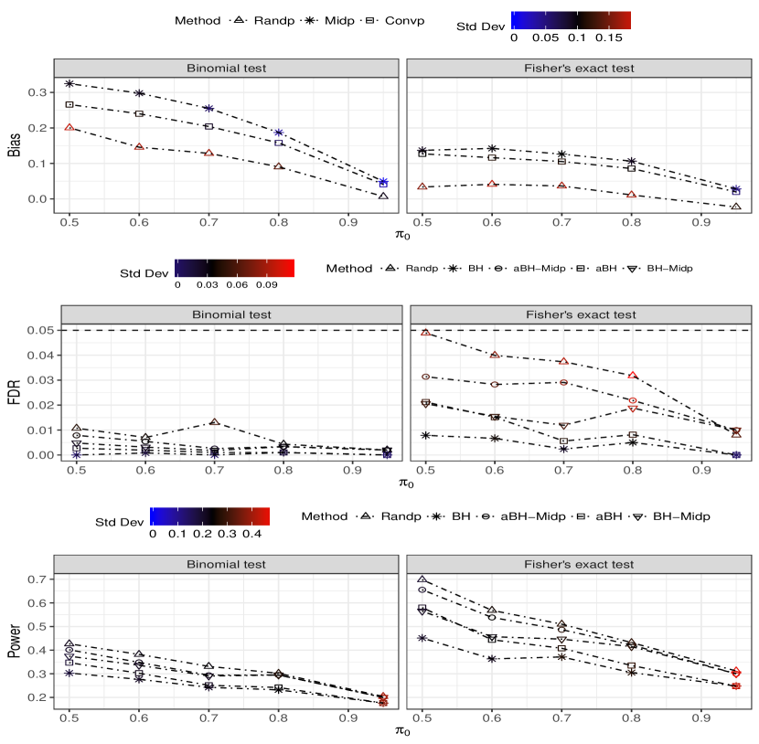
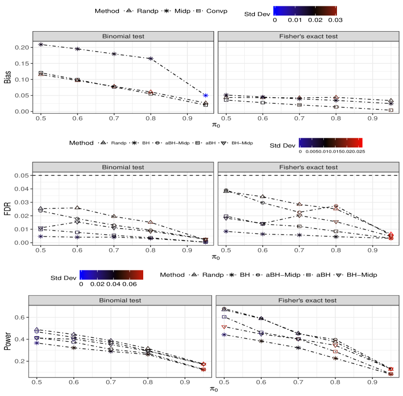
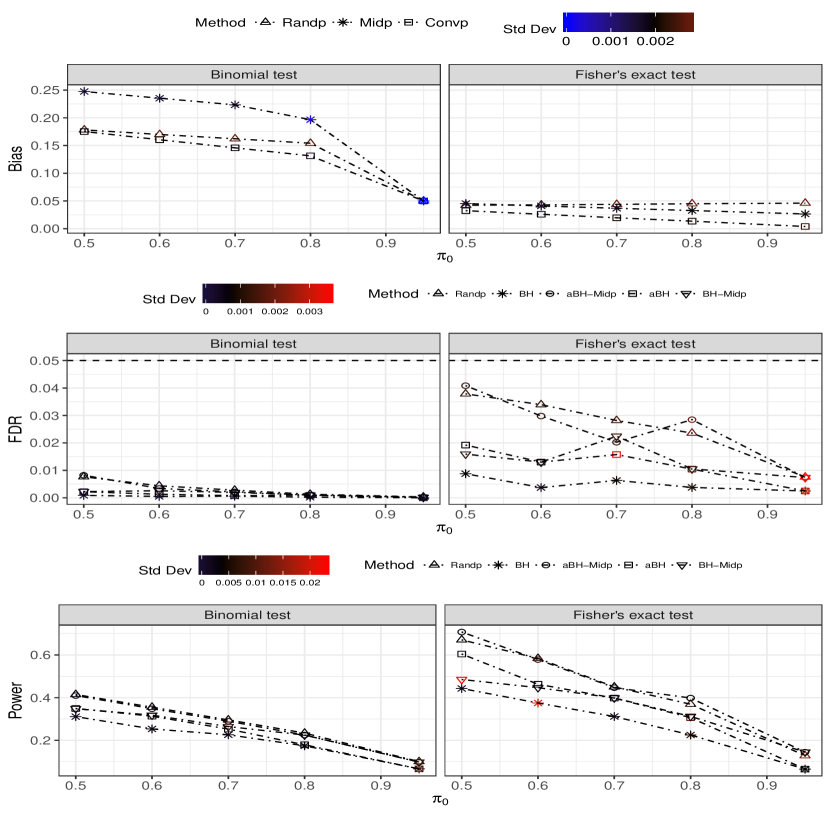
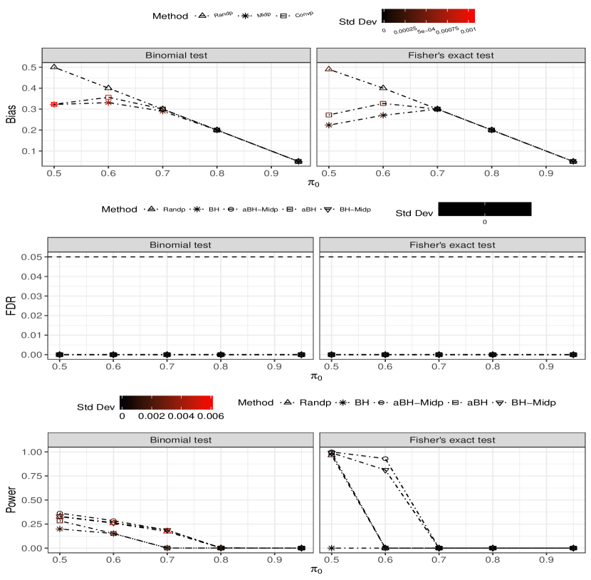
An estimator of the proportion $\pi_{0}$ is better if it is less conservative (i.e., having smaller upward bias), is stable (i.e., having small standard deviation), and induces a conservative adaptive FDR procedure. The top panels of Figure 1, Figure 2, Figure 3, and Figure 4 present the biases and standard deviations of the estimators when they are applied to p-values of BT’s or FET’s. $\hat{\pi}_{0}$ applied to conventional p-values is stable and the most accurate among the estimators, and $\hat{\pi}_{0}^{\text{SARP}}$ has relatively large standard deviation. It is interesting to note that, for Binomial test, $\hat{\pi}_{0}$ applied to two-sided mid p-values may have relatively large bias when $\pi_{0}$ is small.

We use the expectation of the true discovery proportion (TDP), defined as the ratio of the number of rejected false null hypotheses to the total number of false null hypotheses, to measure the power of an FDR procedure. Recall that the FDR is the expectation of the false discovery proportion (FDP). We also report the standard deviations of the FDP and TDP since smaller standard deviations for these quantities mean that the corresponding procedure is more stable in FDR and power. An FDR procedure is better if it is more powerful at the same nominal FDR level and stable.

The middle and bottom panels of Figure 1, Figure 2, Figure 3, and Figure 4 record the FDRs and powers of the procedures respectively. All procedures are conservative. Specifically, in the positive, blockwise dependence setting in our simulation design, the FDRs of the procedures are very close to 00, whereas their powers can be close to $1$ when $\pi_{0}$ is considerably smaller than $1$ but are very close to 00 when $\pi_{0}$ is very close to $1$; see Figure 4. This may be due to the clustering behavior of signals or noise under positive, blockwise correlation for discrete data, and is worth further investigation. The procedures aBH-Midp and SARP have similar power performances and are the most powerful among the procedures in comparison. aBH-Midp is stable but SARP seems to be relatively less stable. The explanation for this is that the conditional expectation of a randomized p-value is the corresponding mid p-value. So, assuming that the $\hat{\pi}_{0}^{\text{SARP}}$ and $\hat{\pi}_{0}$ have similar marginal distributions, the FDP and TDP of aBH-Midp and those of SARP should have similar distributions after averaging out the extra uncertainty induced by the uniform random variable in the definition of a randomized p-value. Note that aBH and BH-Midp have similar power performances. An explanation for this is that the improvement brought by $\hat{\pi}_{0}$ in the adaptive BH procedure applied to conventional p-values can somehow be achieved by applying the BH procedure to mid p-values since a mid p-value is smaller than its corresponding conventional p-value.

5 An application to HIV study

We provide an application of the BH procedure based on two-sided mid p-values to multiple testing based on discrete and heterogeneous p-value distributions in an HIV study. The naming conventions for the procedures compared in the simulation study in Section 4 will be used, and we will only compare BH, BH-Midp, aBH and aBH-Midp. All procedures are implemented at nominal FDR level $0.05$

The study is well described in [12]. The aim of the study is to identify, among $m=118$ positions, the “differentially polymorphic” positions, i.e., positions where the probability of a non-consensus amino-acid differs between two sequence sets. Two sequence sets were obtained from $n=73$ individuals infected with subtype C HIV (and are categorized into Group 1) and $n=73$ individuals with subtype B HIV (and are categorized into Group 2), respectively. How multiple testing is set up based on two-sided p-values of FET’s can be found in [12], where each position on the two sequence sets corresponds to a null hypothesis that “the probabilities of a non-consensus amino-acid at this position are the same between the two sequence sets”.

There are $50$ positions for which the total observed counts are identically $1$ and the corresponding two-sided p-value CDF’s are Dirac masses. To reduce the uncertainty induced by positions whose observed total counts are too small, we only analyze those whose observed total counts are at least $2$. This gives $68$ positions, i.e., $68$ null hypotheses to test. BH makes $15$ discoveries, BH-Midp $16$, aBH $16$ and aBH-Midp $25$, showing the improvement that multiple testing based on mid p-values can bring. The additional discoveries made by the procedures based on mid p-values are worth further investigation, had we been able to prove their conservativeness.

6 Discussion

This paper is motivated by the scope of improving the BH procedure in controlling FDR when it is applied to mid p-values, which has been realized by researchers in multiple testing but no significant progress has been made yet in investigating conditions under which such improvements can be achieved. Considering this procedure with two-sided mid p-values in the contexts of Binomial and Fisher’s exact tests, we have been able to establish sufficient conditions for its conservativeness and provide numerical evidence on its superior performance under these conditions relative to its relevant competitors. Even though these conditions are simple, they depend on the unknown proportion of true null hypotheses. Our study reveals the critical role of this proportion in FDR control for a step-up procedure when p-values are not super-uniform. The conservativeness of the BH procedure based on two-sided mid p-values is also partially due to the existence of sub-intervals on which such a p-value is strictly super-uniform.

Since in practice we often have some information on at least how large the proportion of true nulls is, based on inequality (7), we can rescale the critical constants of the BH procedure so that the modified procedure controls FDR. However, such rescaling very likely will make the critical constants overall smaller than $\left\{i\alpha/m\right\}_{i=1}^{m}$, thus potentially counterbalancing the gain in power of applying the modified BH procedure to mid p-values. In other words, for the multiple testing scenarios considered in this work, it is quite feasible to directly modify the BH procedure to maintain FDR control for mid p-values but possibly at the expense of unimproved power. On the other hand, to develop more powerful MTP’s based on mid p-values whose conservativeness is ensured under weaker conditions than we have presented, a tighter estimate of

$$\xi_{i}=\sum_{r=1}^{m}\frac{e_{i}\left(x_{i}\left(\tau_{r}\right)\right)}{r}\Pr\left(C_{r}^{\left(-i\right)}\right),i\in I_{0},$$ (12)

than given in this paper is needed but usually very hard to obtain. We leave this to future research.

References

  • [1] X. Chen, R. Doerge, A weighted FDR procedure under discrete and heterogeneous null distributions, arXiv:1502.00973v4.
  • [2] Y. Benjamini, Y. Hochberg, Controlling the false discovery rate: a practical and powerful approach to multiple testing, J. R. Statist. Soc. Ser. B 57 (1) (1995) 289–300.
  • [3] J. D. Storey, J. E. Taylor, D. Siegmund, Strong control, conservative point estimation in simultaneous conservative consistency of false discover rates: a unified approach, J. R. Statist. Soc. Ser. B 66 (1) (2004) 187–205.
  • [4] J. D. Habiger, Multiple test functions and adjusted p-values for test statistics with discrete distributions, J. Stat. Plan. Inference 167 (2015) 1–13.
  • [5] H. O. Lancaster, Significance tests in discrete distributions, J. Amer. Statist. Assoc. 56 (294) (1961) 223–234.
  • [6] A. Agresti, Categorical Data Analysis, 2nd Edition, John Wiley & Sons, Inc., New Jersey, 2002.
  • [7] T. Dickhaus, K. Straßburger, D. Schunk, a. I. T. Morcillo-Suarez, Carlos, A. Navarro, How to analyze many contingency tables simultaneously in genetic association studies, Stat. Appl. Genet. Mol. Biol 11 (4).
  • [8] J. T. G. Hwang, M.-C. Yang, An optimality theory for mid p cvalues in $2\times 2$ contingency tables, Statistica Sinica 11 (3) (2001) 807–826.
  • [9] Y. Benjamini, D. Yekutieli, The control of the false discovery rate in mutliple testing under dependency, Ann. Statist. 29 (4) (2001) 1165–1188.
  • [10] S. K. Sarkar, On methods controlling the false discovery rate, Sankhyā: Series A 70 (2) (2008) 135–168.
  • [11] X. Chen, R. W. Doerge, J. F. Heyse, Multiple testing with discrete data: proportion of true null hypotheses and two adaptive FDR procedures, Biometrial Journal 60 (4).
  • [12] P. B. Gilbert, A modified false discovery rate multiple-comparisons procedure for discrete data, applied to human immunodeficiency virus genetics, J. R. Statist. Soc. Ser. C 54 (1) (2005) 143–158.
Refer to caption
Figure 1: Simulation results under independence when $m=20$. The top panel shows results of estimating the true proportion $\pi_{0}$. “Randp” is $\hat{\pi}_{0}^{\text{Randp}}$, “Midp” $\hat{\pi}_{0}^{\text{Midp}}$ and “Convp” $\hat{\pi}_{0}^{\text{Convp}}$. The legend “Std Dev” is the standard deviation of each estimator. The middle panel shows the FDR of each procedure where the legend “Std Dev” is the standard deviation of the FDP, and the bottom the power where the legend “Std Dev” is the standard deviation of the TDP.
Refer to caption
Figure 2: Simulation results under independence when $m=10^{3}$. The top panel shows results of estimating the true proportion $\pi_{0}$. “Randp” is $\hat{\pi}_{0}^{\text{Randp}}$, “Midp” $\hat{\pi}_{0}^{\text{Midp}}$ and “Convp” $\hat{\pi}_{0}^{\text{Convp}}$. The legend “Std Dev” is the standard deviation of each estimator. The middle panel shows the FDR of each procedure where the legend “Std Dev” is the standard deviation of the FDP, and the bottom the power where the legend “Std Dev” is the standard deviation of the TDP.
Refer to caption
Figure 3: Simulation results under independence when $m=10^{5}$. The top panel shows results of estimating the true proportion $\pi_{0}$. “Randp” is $\hat{\pi}_{0}^{\text{Randp}}$, “Midp” $\hat{\pi}_{0}^{\text{Midp}}$ and “Convp” $\hat{\pi}_{0}^{\text{Convp}}$. The legend “Std Dev” is the standard deviation of each estimator. The middle panel shows the FDR of each procedure where the legend “Std Dev” is the standard deviation of the FDP, and the bottom the power where the legend “Std Dev” is the standard deviation of the TDP.
Refer to caption
Figure 4: Simulation results under positive, block dependence when $m=10^{5}$. The top panel shows results of estimating the true proportion $\pi_{0}$. “Randp” is $\hat{\pi}_{0}^{\text{Randp}}$, “Midp” $\hat{\pi}_{0}^{\text{Midp}}$ and “Convp” $\hat{\pi}_{0}^{\text{Convp}}$. The legend “Std Dev” is the standard deviation of each estimator. The middle panel shows the FDR of each procedure where the legend “Std Dev” is the standard deviation of the FDP, and the bottom the power where the legend “Std Dev” is the standard deviation of the TDP.