Detecting coalitions by optimally partitioning signed networks of political collaboration

Abstract

We propose new mathematical programming models for optimal partitioning of a signed graph into cohesive groups. To demonstrate the approach’s utility, we apply it to identify coalitions in US Congress since 1979 and examine the impact of polarized coalitions on the effectiveness of passing bills. Our models produce a globally optimal solution to the NP-hard problem of minimizing the total number of intra-group negative and inter-group positive edges. We tackle the intensive computations of dense signed networks by providing upper and lower bounds, then solving an optimization model which closes the gap between the two bounds and returns the optimal partitioning of vertices. Our substantive findings suggest that the dominance of an ideologically homogeneous coalition (i.e. partisan polarization) can be a protective factor that enhances legislative effectiveness.

Keywords: Signed network, Polarization, Balance theory, Graph partitioning

The reference to this article should be made as follows: Aref, S., and Neal, Z. Detecting coalitions by optimally partitioning signed networks of political collaboration. Scientific Reports, (2020), www.doi.org/10.1038/s41598-020-58471-z.

Old title: Legislative effectiveness hangs in the balance: Studying balance and polarization through partitioning signed networks

Introduction

We propose a general method for identifying cohesive groups in signed networks (networks with positive and negative edges), and apply it to political networks, which have become a common focus in complex network analysis[1, 2, 3]. Specifically, we examine signed networks of political collaboration and opposition to identify the members of polarized coalitions in the US Congress, then use these coalitions to examine the impact of polarization on effectiveness in passing bills.

In legislative bodies where most pairs of legislators co-sponsor bills, a network of who co-sponsors with whom becomes a highly dense network which would not be suitable for studying political alliances, coalitions, and polarization. Instead, we use signed networks [4] created based on significantly many and significantly few co-sponsorships as two types of edges with opposite nature where a stochastic degree sequence model (SDSM) [5] is used as the null model, to define thresholds of “many” and “few.” Previous research [6] on the same data has shown an increase in polarization in the US Congress when measured by the triangle index, which provides a locally-aggregated index of polarization based on structural balance [7]. However, the triangle index only measures the level of balance and polarization, but does not identify the members of the political coalitions that are polarized. For this we turn to the frustration index [8, 9, 10] (also known as the line index of balance [11]), which optimally partitions a signed graph into two opposing but internally cohesive “coalitions” [12]. Substantively, these coalitions [13] represent groups of legislators who sponsor significantly many bills with each other (i.e. are political allies), but who sponsor significantly few bills with those in the other coalition (i.e. are political enemies). In our analyses of legislative effectiveness, we focus on the level of partisanship within the largest, and therefore controlling, coalition.

Computing the frustration index is an NP-hard problem [14], and so is the equivalent partitioning problem that deals with minimizing the total number of intra-group negative and inter-group positive edges. The optimality of a numerical solution to an instance of an optimization problem depends on the function under optimization. Most studies on this topic use heuristic methods for partitioning signed networks under similar objectives [15, 16, 17, 18]. These methods are not guaranteed to provide the optimal solution or even its approximation within a constant factor [14, 19], but can potentially be implemented on larger networks.

Computing the exact value of the frustration index, in principle, involves searching among all possible ways to partition a given signed network into $k\leq 2$ groups in order to find the partitioning which minimizes the total number of intra-group negative and inter-group positive edges. We propose a new method for tackling the intensive computations by providing upper and lower bounds for this number, then solving an optimization model which closes the gap between the two bounds and returns the exact value of frustration index alongside the optimal partitioning of vertices.

Signed graph and balance theory preliminaries

In this section, we recall some basic definitions of signed graphs and balance theory.

Signed graphs

We consider an undirected signed graph $G=(V,E,\sigma)$ where $V$ and $E$ are the sets of vertices and edges respectively, and $\sigma$ is the sign function $\sigma:E\rightarrow\{-1,+1\}$. Graph $G$ contains $|V|=n$ nodes. The set $E$ of edges contains $m^{-}$ negative edges and $m^{+}$ positive edges adding up to a total of $|E|=m=m^{+}+m^{-}$ edges. The signed adjacency matrix and the unsigned adjacency matrix are denoted by A and ${|\textbf{A}|}$ respectively. Their entries are defined in Eq. (3) and Eq. (6).

$$a{{}_{u}}{{}_{v}}=\left\{\begin{array}[]{ll}\sigma_{(u,v)}&\quad\mbox{if }{(u,v)}\in E\\ 0&\quad\mbox{if }{(u,v)}\notin E\end{array}\right.$$ (3)

$$|a{{}_{u}}{{}_{v}}|=\left\{\begin{array}[]{ll}1&\quad\mbox{if }{(u,v)}\in E\\ 0&\quad\mbox{if }{(u,v)}\notin E\end{array}\right.$$ (6)

Balance and cycles

A cycle of length $k$ in $G$ is a sequence of nodes $v_{0},v_{1},...,v_{k-1},v_{k}$ such that for each $i=1,2,...,k$ there is an edge from $v_{i-1}$ to $v_{i}$ and the nodes in the sequence except for $v_{0}=v_{k}$ are distinct. The sign of a cycle is the product of the signs of its edges. A cycle with negative (positive) sign is unbalanced (balanced). A balanced network (graph) is one with no negative cycles.

Balance theory is conceptualized by Heider in the context of social psychology [20]. It was then formulated as a set of graph-theoretic conditions by Cartwright and Harary [21] which define a signed graph to be balanced if all its cycles are positive. Cartwright and Harary also introduce measuring the level of balance using, among other indices, the fraction of positive cycles [21, page 288]. Three years later, Harary suggested using frustration index [11] (under a different name); a measure which satisfies key axiomatic properties [10], but has been underused for decades due to the complexity involving its computation [22, 19, 23].

Evaluating balance and frustration

In this section, we explain our computational approach to analyzing signed networks by providing brief definitions and discussions on measuring balance, frustration and partitioning, and graph optimization models.

Measuring partial balance

Signed networks representing real data are often unbalanced, which motivates measuring the intermediate level of partial balance [10]. The first measure we use is triangle index denoted by $T(G)$ which equals the fraction of positive cycles of length 3 [21, 24]. We use Eq. (7) suggested in [7] for computing triangle index, $T(G)$, in which $\operatorname{Tr}(\textbf{A})$ denotes the trace (sum of diagonal entries) of A.

$$T(G)=\frac{\operatorname{Tr}({\textbf{A}}^{3})+\operatorname{Tr}({|\textbf{A}|}^{3})}{2\operatorname{Tr}({|\textbf{A}|}^{3})}$$ (7)

The other measure we use is the normalized frustration index [10] denoted by $F(G)$ which is based on normalizing the minimum number of edges whose removal results in a balanced graph [25, 11, 8].

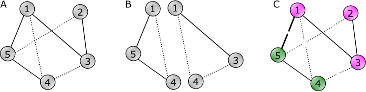
Figure 1: (A) An example signed network. (B) Evaluating balance using triangles. (C) Evaluating balance using frustration.

Fig. 1(A) shows an example signed graph in which the three dotted lines represent negative edges and the four solid lines represent positive edges. The level of balance in this signed graph can be evaluated using triangles (B) or frustration (C). The former approach, (B), involves identifying triangle 1-4-5 as unbalanced and triangle 1-3-4 as balanced leading to the numeric index $T(G)=1/2$. The latter approach, (C), involves finding a partitioning of vertices $\{\{1,2,3\},\{4,5\}\}$ (shown by green and purple colors in Fig. 1) which minimizes the total number of intra-group negative and inter-group positive edges to $1$ (only edge $(1,5)$ according to this partitioning). Note that removing edge $(1,5)$ leads to a balanced signed graph.

Frustration and partitioning

Given signed graph $G=(V,E,\sigma)$, we can partition $V$ into two subsets: $X$ and $V\setminus X$. We let binary variable $x_{i}$ denote the subset which node $i$ belongs to under partitioning $\{X,V\setminus X\}$, where $x_{i}=1$ if $i\in X$ and $x_{i}=0$ otherwise.

A positive edge $(i,j)\in E^{+}$ is said to be frustrated if its endpoints $i$ and $j$ belong to different subsets ($x_{i}\neq x_{j}$). A negative edge $(i,j)\in E^{-}$ is said to be frustrated if its endpoints $i$ and $j$ belong to the same subset ($x_{i}=x_{j}$). We define the frustration count $f_{G}(X)$ as the number of frustrated edges of $G$ under partitioning $\{X,V\setminus X\}$:

$$f_{G}(X)=\sum_{(i,j)\in E}f_{ij}(X)$$

where $f_{ij}(X)$ is the frustration state of edge $(i,j)$, given by

$$f_{ij}(X)=\begin{cases}0,&\text{if}\ x_{i}=x_{j}\text{ and }(i,j)\in E^{+}\\ 1,&\text{if}\ x_{i}=x_{j}\text{ and }(i,j)\in E^{-}\\ 0,&\text{if}\ x_{i}\neq x_{j}\text{ and }(i,j)\in E^{-}\\ 1,&\text{if}\ x_{i}\neq x_{j}\text{ and }(i,j)\in E^{+}.\\ \end{cases}$$ (8)

The frustration index of a graph $G$ can be computed exactly by finding partitioning $X^{*},V\setminus X^{*}\subseteq V$ of $G$ that minimizes the frustration count $f_{G}(X)$, i.e.  solving Eq. (9) [22, 19].

$$L(G)=\min_{X\subseteq V}f_{G}(X)\$$ (9)

The normalized frustration index, $F(G)$, is computed based on $L(G)$ and according to Eq. (10) which allows measuring the level of partial balance based on numerical values within the unit interval ($m$ denotes the number of edges).

$$F(G)=1-2L(G)/m$$ (10)

One may notice some similarities between the problem of finding communities in unsigned networks [26, 27, 28, 29, 30, 31] and that of partitioning signed networks to minimize the frustration count. One key difference is that in the latter problem for every pair of vertices there are three cases (as opposed to two): a positive edge, a negative edge, or no edge between the two vertices. Due to the differences between objectives of these two problems (minimizing frustration count as opposed to maximizing modularity or other quantities), the partitioning obtained from running community detection algorithms on positive edges of a signed graph will not generally minimize the frustration count.

Recent studies on frustration index and signed networks suggest [22, 19] and implement [23] efficient graph optimization models to compute the frustration index of relatively large (up to $10^{5}$ edges) sparse networks. However, the signed networks we analyze have substantially higher densities compared to the instances in [22, 19, 23]. This requires developing new computational models for tackling the intensive computations involved in obtaining the frustration index of dense graphs.

Bounding the frustration index

In this subsection, we discuss obtaining lower and upper bounds for the frustration index. Using these bounds is a way of substantially reducing the running time, but theoretically they are not required.

The linear programming relaxation (LP relaxation) of the binary optimization models in [22, 19] can be used to compute a lower bound for the frustration index. The linear programming model in Eq. (11) is developed for this purpose.

$$\begin{split}\min_{x_{i},x_{ij}}Y=&\sum\limits_{(i,j)\in E^{+}}x_{i}+x_{j}-2x_{ij}+\sum\limits_{(i,j)\in E^{-}}1-(x_{i}+x_{j}-2x_{ij})\\ \text{s.t.}\quad x_{ij}&\leq(x_{i}+x_{j})/2\quad\forall(i,j)\in E^{+}\\ x_{ij}&\geq x_{i}+x_{j}-1\quad\forall(i,j)\in E^{-}\\ x_{i}+x_{jk}&\geq x_{ij}+x_{ik}\quad\forall(i,j,k)\in T\\ x_{j}+x_{ik}&\geq x_{ij}+x_{jk}\quad\forall(i,j,k)\in T\\ x_{k}+x_{ij}&\geq x_{ik}+x_{jk}\quad\forall(i,j,k)\in T\\ 1+x_{ij}+x_{ik}+x_{jk}&\geq x_{i}+x_{j}+x_{k}\quad\forall(i,j,k)\in T\\ x_{i}&\in[0,1]\quad\forall i\in V\\ x_{ij}&\in[0,1]\quad\forall(i,j)\in E\end{split}$$ (11)

In Eq. (11), $T=\{(i,j,k)\in V^{3}\mid(i,j),(i,k),(j,k)\in E\}$ is the set which contains ordered 3-tuples of nodes whose edges form a triangle in $G$. The continuous linear programming model in Eq. (11) is developed by combining the LP relaxation of the 0/1 linear model in [22][Subsection 4.3] and the triangle constraints in [22][Subsection 4.4]. It follows from the LP relaxation that the optimal solution $Y^{*}$ to the model in Eq. (11) is a lower bound for the frustration index $Y^{*}\leq L(G)$.

Any given partitioning $\{X,V\setminus X\}$ for signed graph $G$ is associated with a frustration count $f_{G}(X)$ which is by definition (as in Eq. (9)) an upper bound for the frustration index

$$f_{G}(X^{*})=L(G)\leq f_{G}(X)\quad\forall X\subseteq V.$$

We use a specific partitioning $\{X^{\prime},V\setminus X^{\prime}\}$ as a starting point to “warm-start” the algorithm for computing the frustration index. Partitioning $\{X^{\prime},V\setminus X^{\prime}\}$ groups nodes into two subsets based on the party affiliation of legislators. To be more precise, for node $i$ which represents a legislator, decision variable $x_{i}$ is given initial value $0$ if the reciprocal legislator is a Democrat and $x_{i}$ is given initial value $1$ otherwise.

Computing the frustration index

After bounding the frustration index, we use the binary linear programming model in Eq. (12) which minimizes the number of frustrated edges.

$$\begin{split}\min_{x_{i},f_{ij}}Z&=\sum\limits_{(i,j)\in E}f_{ij}\\ \text{s.t.}\quad f_{ij}&\geq x_{i}-x_{j}\quad\forall(i,j)\in E^{+}\\ f_{ij}&\geq x_{j}-x_{i}\quad\forall(i,j)\in E^{+}\\ f_{ij}&\geq x_{i}+x_{j}-1\quad\forall(i,j)\in E^{-}\\ f_{ij}&\geq 1-x_{i}-x_{j}\quad\forall(i,j)\in E^{-}\\ \sum\limits_{(i,j)\in E}f_{ij}&\geq Y^{*}\\ x_{i}&\in\{0,1\}\quad\forall i\in V\\ f_{ij}&\in\{0,1\}\quad\forall(i,j)\in E\end{split}$$ (12)

The binary variables of the model are $f_{ij}\>\forall(i,j)\in E$ which denotes frustration of edge $(i,j)$ and $x_{i}\>\forall i\in V$ which denotes the subset of node $i$. To warm-start the algorithm which solves Eq. (12), we initialize $x_{i}$ variables based on partitioning $\{X^{\prime},V\setminus X^{\prime}\}$. The model in Eq. (12) is developed by combining the XOR model in [19][Subsection 3.2] with an additional constraint to incorporate the lower bound $Y^{*}$ obtained from Eq. (11). We implement the speed-up techniques discussed in [19] and solve the binary linear programming model in Eq. (12) using Gurobi solver (version 8.0) [32] on a virtual machine with 32 Intel Xeon CPU E5-2698 v3 @ 2.30 GHz processors and 32 GB of RAM running 64-bit Microsoft Windows Server 2012 R2 Standard.

Results

In this section, we provide the results of analyzing balance and frustration in signed networks of US Congress legislators.

Partial balance, frustration, and optimal partitioning

We evaluate the level of partial balance using two different methods. Fig. 2 illustrates partial balance in the signed networks of the US Congress over time measured by the triangle index and normalized frustration index. Values of the two measures, the triangle index $T(G)$ and the normalized frustration index $F(G)$, are highly correlated (correlation coefficients are $0.95$ and $0.91$ respectively for House and Senate networks) and both show relatively high levels of partial balance which have increased in the time period 1979-2016. The results in Fig. 2 indicate an increase in the polarization of both chambers of US Congress, which is in accordance with the literature [33, 34, 35, 36, 6]. Although the triangle index $T(G)$ and the normalized frustration index $F(G)$ capture very similar information concerning the level of partial balance, only the computation of $F(G)$ also provides the partitioning that minimizes the sum of intra-group negative and inter-group positive edges.

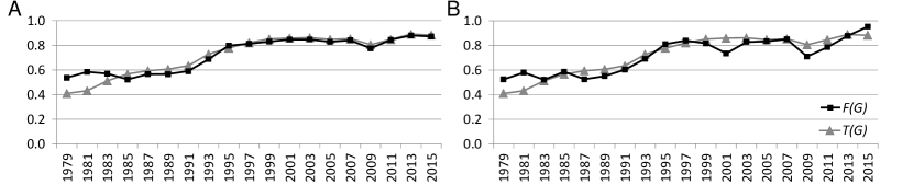
Figure 2: Two measures of partial balance indicating an overall increase in political polarization in (A) US House of Representatives and (B) US Senate over the time period 1979-2016

Solving the continuous optimization model in Eq. (11) and the discrete (binary) optimization model in Eq. (12) requires intensive computations for large instances such as signed networks of the House. Given the size and density of these instances, the models in Eq. (11) and Eq. (12) have thousands of variables and possibly millions of constraints requiring a high performance computer taking advantage of parallel computing capabilities [23].

For example, the signed graph instance of the 113th House session has $m=75,771$ edges and $|T|=7,102,625$ triangles which result in a total of $m+4|T|=28,486,271$ constraints for the model in Eq. (11). Gurobi solver takes $5300$ seconds (around 1.5 hours) to solve the model in Eq. (11) to global optimality and return $Y^{*}$, the lower bound for the frustration index. For the same instance, the discrete optimization model in Eq. (12) has $n+m=76,218$ binary variables and $2m+1=151,543$ constraints. This large instance takes $43,523$ seconds (around 12 hours) for Gurobi to reach global optimality and return the frustration index and the partitioning of the nodes. In total for the 113th session of the House, it takes $48,823$ seconds (around 13.5 hours) to compute the exact value of the frustration index which is the longest solve time among all instances. The average computation time for House instances is $17,763$ seconds (around 5 hours) and the standard deviation is $15,411$ seconds (around 4.5 hours). For Senate instances, the average computation time is 4 seconds and the standard deviation is 6 seconds.

Using the optimal values of the $x_{i}$ variables obtained by solving the discrete optimization model in Eq. (12), we partition nodes of each network into two groups (subsets $X^{*}$, $V\setminus X^{*}$). For each signed network, either $X^{*}$ or $V\setminus X^{*}$ has the larger set cardinality and therefore represents the largest coalition for the corresponding session.

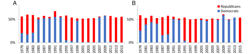
Figure 3: The number of legislators from the two main parties who belong to the controlling coalition indicating an increase in the partisan homogeneity of the controlling coalition in (A) US House of Representatives and (B) US Senate over the time period 1979-2016

We evaluate the composition of the largest and therefore controlling coalitions in each session and chamber based on the party affiliation of its legislators. Fig. 3 illustrates the number of legislators from the two main political parties in the controlling coalitions of the US Congress. As it can be seen in Fig. 3, the controlling coalitions have become more homogeneous (i.e. partisan) over the time period 1979-2016.

Legislative effectiveness and polarization in the US congress

Within the field of comparative US politics, two topics attract particular attention at the federal level: legislative effectiveness and political polarization. Legislative effectiveness refers to the ability of individual legislators [37, 38], or of an entire legislative body [39], to advance their agenda, typically by facilitating the passage of legislation. Political polarization (when applied to elected officials or “elites”) refers to the formation of non-overlapping ideologically homogeneous groups [33, 6]. When these groups mirror political party affiliations, it is also called partisan polarization. For several decades, legislative effectiveness in the US has declined (as illustrated in Fig. 4), while partisan polarization has increased [6]. These trends have led many to hypothesize that they are related, and specifically that “unified party control has [not] been legislatively more productive than divided party control” [40, xii]. Based on the legislative process used by the US Congress, it might be expected that a chamber’s bills are more likely to become law when the controlling party holds a larger majority, because its members can form a voting bloc. However, the analysis in the next section suggests that that changes in bill passage rates are better explained by the partisanship of a chamber’s largest coalition.

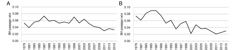
Figure 4: The fraction of bills that eventually become law (bill passage rate) indicating legislative effectiveness in (A) US House of Representatives and (B) US Senate over the time period 1979-2016

Mediation in bill passage

Using a bivariate linear regression, we find that the percentage of bills introduced in a chamber that become law (passage rate) significantly declines over time. The passage rate has declined in the House by an average of $0.11$ percentage points each session ($\beta=-0.528,p<0.05$), and in the Senate by an average of $0.35$ percentage points each session ($\beta=-0.852,p<0.01$; see Fig. 5(A)). We report standardized coefficients ($\beta$) to facilitate cross-model comparisons. The percentage point changes are unstandardized bivariate regression coefficients, reported here for context. These variations in passage rate are not simply a function of the total number of bills introduced (House: $r=-0.29,p=0.22$; Senate: $r=-0.08,p=0.74$), which exhibit no association with time (House: $r=-0.34,p=0.15$; Senate: $r=0.19,p=0.43$; see tables S2 and S4).

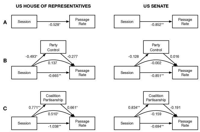
Figure 5: Predicting the rate of bill passage in the US House of Representatives and Senate; Standardized coefficients are reported; $**p<.01,*p<.05$. (A) Over time, the passage rate has declined. (B) The decline is not mediated by changes in the size of a party’s majority in a chamber. (C) In the House, but not the Senate, it is mediated by the partisan homogeneity in the controlling coalition.

To investigate possible explanations for variations in passage rate, we estimate two separate structural equation models for each chamber. A commonsense model tests the expectation that when the majority party holds a larger numerical majority, they should have greater success passing bills [41]. The key variable in this model, party control, is defined as the absolute difference between the number of Republicans and Democrats. Computing party control does not require any information about the legislators’ network. We find no support for this model; party control does not mediate the relationship between time and passage rate. (see Fig. 5(B)).

A more nuanced model tests the expectation that when the controlling coalition is more partisan and thus more ideologically unified, it will have greater success passing bills. The key variable in this model, coalition partisanship, is defined as the fraction of non-independent members in the largest coalition that affiliate with that coalition’s dominant political party (see Fig. 3). We compute coalition partisanship by applying the partition method described above to a signed network of political collaboration and opposition. We find support for this model in the US House, but not the US Senate (see Fig. 5(C)). Specifically, we find that in the House, the partisan homogeneity of the controlling coalition has increased over time ($\beta=0.771,p<.01$), which is consistent with past findings concerning polarization [6], and that coalition homogeneity increases passage rates ($\beta=0.661,p<0.05$), which is consistent with our expectation about the impact of ideological unity. Together, these effects imply a significant and positive indirect effect of time on the passage rate ($\beta=0.510,p<.05$), mediated by coalition partisanship. Thus, the observed decline in bill passage rates in the US House would have been worse (direct effect: $\beta=-1.038,p<.01$), but was mitigated by increasingly ideologically homogeneous coalitions, which are a protective factor against declines in legislative effectiveness.

Summary and conclusions

In this study we proposed a general method for identifying internally cohesive opposing coalitions in signed networks of legislators based on structural balance theory, then applied this method to identify opposing coalitions in the US Congress, showing that these coalitions’ partisanship can explain changes in legislative effectiveness better than political parties. Based on this analysis, we offer a series of substantive and methodological conclusions.

Consistent with prior studies [33, 34, 35, 36, 6], we find that polarization has increased in both the US Senate and US House of Representatives, and that this polarization has largely mirrored partisan divisions along political party lines. We operationalized polarization using the level of a signed graph’s structural balance, and therefore measure what [6] calls “strong polarization,” but have used two different measures of balance. We find that the two measures are highly correlated and both support the conclusion of increasing polarization.

The triangle index is easy to compute, but provides only a locally-aggregated measure of a graph’s level of balance. In contrast, computing the frustration index is difficult, but it provides not only a global measure of a graph’s level of balance, but also the optimal partitioning of vertices into internally cohesive but mutually antagonist groups. We have demonstrated a practical method for computing the exact value of frustration index and identifying the optimal partition in dense graphs of $|E|\gg 50000$ that involves first obtaining upper and lower bounds, using exogenous node properties (e.g. legislators’ political party affiliations), and solving a large-scale binary linear programming model. In the context of legislative networks, this method allows us to identify the most cohesive coalitions of legislators under conditions of balance theory.

Although our computational innovations make the identification of internally cohesive opposing coalitions practically feasible, we must also demonstrate that these coalitions are more informative than other simpler grouping possibilities. In the legislative context, we show that the partisan composition of these cohesive coalitions better explains the declining legislative effectiveness in the US House of Representatives than simply examining legislators’ political party affiliations. This affirms Mayhew’s claim that “no theoretical treatment of the United States Congress that posits parties as analytic units will go very far” [42, p.27] but goes a step further by identifying an alternative analytic unit – internally cohesive opposing coalitions – that does have explanatory power. Importantly, coalitions appear useful only for explaining the legislative effectiveness of the House, but not the Senate. However, this is also consistent with existing political science theory that “the lack of majority control of [procedural] processes in the Senate negates the possibility of significant party [or other group-based] effects in that body” [43, p.7]. Therefore, in general terms, our empirical findings suggest that in legislative bodies where a sufficiently large group of legislators can influence procedural processes, the composition of the largest coalition is more important than the size of the majority party’s majority. This is perhaps obvious in parliamentary systems where multi-party coalition forming is essential, but is noteworthy in the non-parliamentary US Congress.

These conclusions have some significant implications for both the future study of signed networks, and of the link between polarization and legislative effectiveness. First, by providing a practical method for computing the frustration index of relatively dense graphs, we hope to move the study of signed graphs beyond merely determining the level of balance, and toward the study of how the composition of mostly opposing groups impact other network dynamics. Second, our empirical findings suggest that research on polarization and its impact on the legislative process should look beyond political parties and partisanship to more subtle but influential forms of coordination, such as internally cohesive coalitions which are antagonist towards one another.

Materials and Methods

Relations of collaboration and opposition between elected officials are difficult to collect directly because politicians have limited time to participate in surveys and have good reasons to conceal their true political relations. Therefore, studies of elected officials’ political networks typically measure these relations indirectly, using bipartite projections focusing on their co-sponsorship of bills [44], co-voting on bills [36, 45, 46], co-membership on committees [47], and co-attendance at press events [48]. For a range of substantive reasons noted by [6] (e.g. relatively few bills are actually voted on, committee memberships are driven by such non-ideological factor such as seniority), we examine political relations from bill co-sponsorship.

Specifically, we use a signed network of inferred political relations among the members of the US House of Representatives, and among the members of the US Senate, in each session of Congress from 1979 to 2016 (96th session – 114th session). The process for creating these signed networks is described in detail by [6] and they are available in a public Figshare data repository [4].

Inferring signed networks from co-sponsorship data

Importantly, all pairs of legislators co-sponsor at least some of the same bills, so we know that the mere existence of some co-sponsorships does not imply they collaborate, and that some number of co-sponsorships can actually indicate avoidance. In previous work [6], a stochastic degree sequence model (SDSM) [5] is used to define thresholds of significantly few and significantly many co-sponsorships by building the empirical sampling distribution of two legislators’ joint co-sponsorships under a null model in which each legislator co-sponsored approximately the same number of bills and each bill received approximately the same number of co-sponsorships (i.e. holding approximately constant the legislator and bill degree sequence). To be more specific, given a bipartite graph $B$, Monte Carlo methods can be used to generate probability distributions $BB^{\prime}_{ij}$ when $Pr(B_{ij}=1)$ is a function of the row and column marginals of $B$ [6]. Decisions about whether a given dyad represents significantly few or significantly many co-sponsorships are made by comparing their observed number of joint co-sponsorships to the empirical sampling distribution using a two-tailed $\alpha=0.05$ threshold. For example, Fig. 6 shows that Rep. Earl Blumenhauer (D-OR3) and Rep. Sheila Jackson-Lee (D-TX18) were observed to have co-sponsored 242 of the same bills (dashed vertical line). The magnitude of joint co-sponsorships, and the fact that both representatives are Democrats, might lead one to conclude that they are collaborating. However, the shaded distribution shows the expected number of joint co-sponsorships under the SDSM null model in which each representative randomly chooses which bills to co-sponsor. Comparing these representatives’ observed number of joint co-sponsorships to the null model expectation, we find that they co-sponsor significantly fewer of the same bills than would be expected at random and therefore define the edge between them as negative.

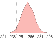
Figure 6: The observed number of co-sponsorships and the null model sampling distribution obtained using the SDSM for Rep. Earl Blumenhauer (D-OR3) and Rep. Sheila Jackson-Lee (D-TX18)

This approach differs from other methods of reducing weighted graphs to binary or signed graphs [49, 50] because it explicitly incorporates information from the original bipartite data (i.e. legislators linked to bills), thereby ensuring it is not lost when these data are projected as a unipartite graph. Additionally, [6] extracts signed backbone networks rather than the weighted bipartite projections because the weights in those projections are distorted by heterogeneity in the bipartite degree sequences (i.e. some legislators sponsor many bills, others sponsor few; [51, 5]).

Although data on earlier sessions are available, they were excluded because prior to the 96th session, House rules imposed a limit of 25 co-sponsors per bill, which artificially distorts co-sponsorship patterns and limits the usefulness of these data for inferring political networks [52]. These data do not distinguish between a bill’s “sponsor” and its “co-sponsors” because the former is simply the legislator whose name appears first in a potentially long list of legislators responsible for the bill’s introduction.

Although these data represent a time-series of legislative interactions, we examine the networks cross-sectionally for two reasons. First, there are a large number of joiners and leavers in each new session as incumbents lose their seats, freshmen join Congress, or representatives become senators, making most dynamic models impractical to estimate. Second, although some political relationships develop over long periods of time, the effectiveness of any particular session of Congress can be evaluated independently.

Availability of data and code

All the data and codes used in this study are publicly available with links and descriptions provided in the supplementary information.

Author contributions

S.A. developed and implemented new methods and algorithms, obtained the results, and prepared supplementary information; Z.N. prepared network data, ran statistical models, and analyzed the results; both authors contributed to designing and conducting the research and writing the paper.

Additional Information

The authors declare neither financial nor non-financial competing interests.

Supplementary information for
Detecting coalitions by optimally partitioning signed networks of political collaboration

This document describes all materials and methods for the article “Detecting coalitions by optimally partitioning signed networks of political collaboration” by Samin Aref and Zachary Neal.

Supplementary Information:

Supplementary Text
Figs. 7 to 10
Tables 1 to 4
Captions for Movies S1 to S2
Captions for Databases S1 to S2
References (53-58)

Other Supplementary Materials for this manuscript include the following:

Movies S1 to S2
Databases S1 to S2

Supplementary Text

Data availability

All network data and numerical results related to this study are publicly available with links provided in this document. The code for the optimization models used is this study is publicly available on a Github repository.

Analyzing networks of legislators

Most research on performance of political systems, and on the link between polarization and legislative effectiveness, has focused on legislators’ ideological positions [53], role of political parties [54, 55], and majority party size [41] within legislative chambers. However, others have suggested that a focus on parties to explain the dynamics of the US Congress is misguided [42]. Parties are administrative conveniences that facilitate coordination and often serve as a useful heuristic for their members’ ideology, but because party affiliation is different from ideological position, a focus on political parties oversimplifies matters by assuming within-party ideological homogeneity and between-party ideological heterogeneity. Therefore, in this paper, we adopt a different approach, focusing more on networks of collaborations between legislators during a two-year session and less on legislators’ political party affiliations. We find that this approach – examining polarization from the perspective of networks and structural balance – offers a better explanation of legislative effectiveness than political parties.

Our method of analysis is different from the conventional methods of indexing legislators partisanship [56, 57, 58] which place each legislator on a scale of liberal to conservative. These methods are shown to produce results correlating with important historical events in the US politics and therefore are standard practice in quantifying polarization [45]. While these methods indicate the political climate as a whole, they are not designed to take network relations of legislators into account.

Statistical analysis

The models shown in Fig. 5 (of the article) and discussed in the “Mediation in bill passage” section were estimated using Stata SE 13.1. All models were estimated separately for the US House of Representative and US Senate, and only standardized coefficients are reported. Model A was estimated as an ordinary bivariate linear regression using the following code in Stata software (release 13).

reg rate session, beta

Models B and C were estimated as structural equation models with maximum likelihood estimation using the following codes.

sem (party <- session) (rate <- party session)
sem (coalition <- session) (rate <- coalition session)

This estimation approach allows us to explicitly estimate the total indirect effect of time mediated by party control (in model B) or coalition partisanship (model C), and thus to test whether these variables help explain observed declines in bill passage rates.

Solving the continuous and discrete optimization models

The proposed continuous optimization model can be solved by any mathematical programming solver which supports linear programming (LP) models. In the Github repository, we explain using Gurobi solver (version 8.0) for solving the proposed LP model. The proposed discrete optimization model can be solved by any mathematical programming solver which supports 0/1 linear programming (binary linear) models. In the Github repository, we share our code for using Gurobi solver (version 8.0) to solve the proposed binary linear model.

The code for both the continuous and the discrete optimization models is available on a Github repository at https://github.com/saref/frustration-index-dense.

Using Gurobi for solving mathematical programming models

Our proposed algorithms are developed in Python 3.7 based on the mathematical programming models in [22, 19] for computing the frustration index.

These optimization algorithms are distributed under an Attribution-NonCommercial-ShareAlike 4.0 International (CC BY-NC-SA 4.0) license. This means that one can use these algorithms for non-commercial purposes provided that they provide proper attribution for them by citing [22, 19] and the current article. Copies or adaptations of the algorithms should be released under the similar license.

The following steps outline the process for academics to install the required software (Gurobi solver [32]) on your computer to be able to run the optimization algorithms:

1. Download and install Anaconda (Python 3.7 version) which allows you to run a Jupyter code. It can be downloaded from https://www.anaconda.com/distribution/. Note that you must select your operating system first and download the corresponding installer.

2. Register for an account on gurobi.com/registration-general-reg/ to get a free academic license for using Gurobi. Note that Gurobi is a commercial software, but it can be registered with a free academic license if the user is affiliated with a recognized degree-granting academic institution. This involves creating an account on Gurobi website to be able to request a free academic license in step 5.

3. Download and install Gurobi Optimizer (versions 8.0 and above are recommended) which can be downloaded from https://www.gurobi.com/downloads/gurobi-optimizer-eula/ after reading and agreeing to Gurobi’s End User License Agreement.

4. Install Gurobi into Anaconda. You do this by first adding the Gurobi channel to your Anaconda channels and then installing the Gurobi package from this channel.

   From a terminal window issue the following command to add the Gurobi channel to your default search list

   Ψconda config --add channels http://conda.anaconda.org/gurobi
   Ψ
   

   Now issue the following command to install the Gurobi package

   Ψconda install gurobi
   Ψ
   

5. Request an academic license from gurobi.com/downloads/end-user-license-agreement-academic/ and install the license on your computer following the instructions given on Gurobi license page.

   Completing these steps is explained in the following links (for version 8.1):

   for Windows https://www.gurobi.com/documentation/8.1/quickstart_windows/installing_the_anaconda_py.html,

   for Linux gurobi.com/documentation/8.1/quickstart_linux/installing_the_anaconda_py.html, and

   for Mac gurobi.com/documentation/8.1/quickstart_mac/installing_the_anaconda_py.html.

   After following the instructions above, open Jupyter Notebook which takes you to an environment (a new tab on your browser pops up on your screen) where you can open the main code (which is a file with .ipynb extension).

Visualization of opposing coalitions in Senate networks (Figures 7 to 9)

Figs. 7–9 show the opposing coalitions in three selected Senate networks. Green and orange edges represent significantly many and significantly few co-sponsorships respectively. Blue and red nodes represent Democratic- and Republican-affiliated legislators respectively and nodes for independent legislators are shown in gray.

In Fig. 7, the network has a low level of balance $F(G)=0.524$ (low polarization) and the larger coalition is relatively heterogeneous, which is reflected in the relatively small value of coalition control ($0.559$). In Fig. 8, the network has a low level of balance $F(G)=0.603$ (low polarization) and the larger coalition is relatively homogeneous, which is reflected in the relatively high value of coalition control ($0.911$). In Fig. 9, the network has a high level of balance $F(G)=0.953$ (high polarization) and the larger coalition is homogeneous (coalition control equals $0.981$). The level of balance (coalition control) can also be observed from the colors of the edges (nodes) in Figs. 7–9.

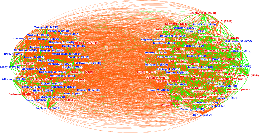
Figure 7: Opposing coalitions in the 96th session of the US Senate (1979). This network shows low balance and low coalition control.

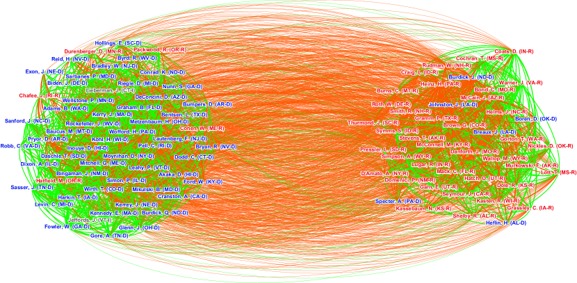
Figure 8: Opposing coalitions in the 102th session of the US Senate (1991). This network shows low balance and high coalition control.

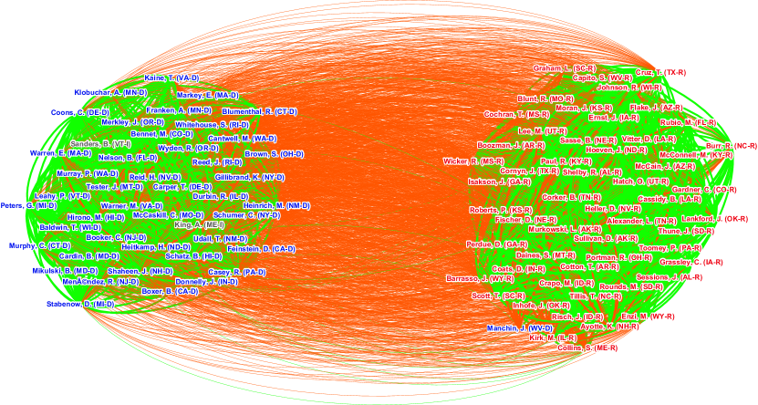
Figure 9: Opposing coalitions in the 114th session of the US Senate (2015). This network shows high balance and high coalition control.

Size of controlling coalitions

Using the optimal values of the $x_{i}$ variables obtained by solving the discrete optimization model, we partition nodes of each network into two groups (subsets $X^{*}$, $V\setminus X^{*}$), namely nodes associated with $x_{i}$ variables taking value $0$ in the optimal solution and nodes whose corresponding variables take value $1$ in the optimal solution.

For each signed network, either $X^{*}$ or $V\setminus X^{*}$ has the larger set cardinality and therefore represents the largest coalition for the corresponding session. Fig. 10

shows the size of the largest and therefore controlling coalitions (winning coalitions [13]) in each signed network alongside the number of Democrats and Republicans in each session for both chambers.

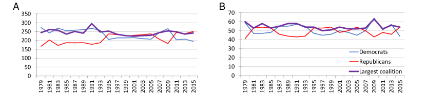
Figure 10: The number of legislators from the two main parties and the size of the largest coalition in (A) US House of Representatives and (B) US Senate over the time period 1979-2016

The controlling coalitions that our partitioning algorithm produces seem to be consistent with Riker’s theory of minimum winning coalitions [13] which argues that politicians try to form winning (larger than majority limit) coalitions which are cohesive and minimal in size.

Legislative effectiveness

We compute our central outcome, legislative effectiveness, as the fraction of bills introduced in a chamber that are eventually signed into law by the president. Tables 2 and 4 report the number of bills introduced in the respective chamber and the number of these bills signed into law, as well as the passage rate, which measures legislative effectiveness. As the values in Tables 2 and 4 illustrate, the passage rate has generally declined over time. Importantly, this is not simply due to the introduction of more frivolous bills and thus is not a simple function of an increase in the denominator (i.e. bills introduced), which has fluctuated around a mean of 3386 in the Senate and 6483 in the House.

Additional numerical results for the Senate and House networks (Tables 1 to 4)

Table 1: Detailed properties and results for Senate networks

Session	Year	$n$	$m$	density	$m^{-}$	$m^{+}$	$T(G)$	$F(G)$	$L(G)$	$Y^{*}$
96	1979	101	2275	0.450	1870	405	0.410	0.524	541	541
97	1981	101	2073	0.410	1639	434	0.432	0.580	435	435
98	1983	101	2194	0.434	1676	518	0.511	0.521	525	525
99	1985	101	2177	0.431	1642	535	0.566	0.586	451	451
100	1987	101	2143	0.424	1535	608	0.594	0.525	509	509
101	1989	101	2445	0.484	1666	779	0.606	0.551	549	549
102	1991	102	2479	0.481	1768	711	0.635	0.603	492	492
103	1993	101	2257	0.447	1633	624	0.728	0.691	349	349
104	1995	102	2324	0.451	1715	609	0.777	0.811	220	220
105	1997	100	3002	0.606	2112	890	0.821	0.839	241	241
106	1999	102	2930	0.569	2108	822	0.852	0.816	269	269
107	2001	101	2522	0.499	1844	678	0.859	0.735	334	334
108	2003	100	2387	0.482	1759	628	0.862	0.828	205	205
109	2005	101	2823	0.559	2048	775	0.848	0.834	235	235
110	2007	102	2779	0.540	1934	845	0.853	0.851	207	207
111	2009	109	3645	0.619	2692	953	0.806	0.710	528	528
112	2011	101	3914	0.775	2693	1221	0.847	0.786	418	418
113	2013	105	3932	0.720	2554	1378	0.890	0.877	241	241
114	2015	100	3696	0.747	2261	1435	0.884	0.953	86	86

Table 2: Democrats (Dems), Republicans (Reps), controlling coalitions (CC), and bill passage in the Senate

Session	Dems	Reps	Size of CC	Dems in CC	Reps in CC	Party control	Coalition control	Bills introduced	Signed into law	Passage rate
96	59	41	60	26	33	18	0.559	3480	257	0.074
97	47	53	53	39	14	6	0.736	3396	210	0.062
98	47	54	58	44	14	7	0.759	3455	283	0.082
99	48	53	53	41	12	5	0.774	3386	304	0.090
100	55	46	55	16	39	9	0.709	3319	299	0.090
101	55	44	58	18	40	11	0.690	3659	277	0.076
102	57	43	58	51	5	14	0.911	3736	198	0.053
103	55	44	54	49	3	11	0.942	2801	172	0.061
104	47	53	54	4	50	6	0.926	2264	81	0.036
105	45	53	50	0	50	8	1.000	2715	141	0.052
106	46	54	51	0	51	8	1.000	3343	194	0.058
107	50	48	54	49	3	2	0.942	3234	71	0.022
108	48	50	52	47	3	2	0.940	3077	148	0.048
109	45	54	52	1	51	9	0.981	4163	151	0.036
110	50	50	53	49	2	0	0.961	3787	142	0.037
111	64	43	63	59	2	21	0.967	4101	120	0.029
112	51	48	52	49	1	3	0.980	3767	79	0.021
113	57	46	56	54	0	11	1.000	3067	77	0.025
114	44	54	54	1	53	10	0.981	3589	108	0.030

Table 3: Detailed properties and results for House networks

Session	Year	$n$	$m$	density	$m^{-}$	$m^{+}$	$T(G)$	$F(G)$	$L(G)$	$Y^{*}$
96	1979	442	51081	0.524	43097	7984	0.410	0.536	11845	11845
97	1981	447	49364	0.495	40304	9060	0.432	0.584	10260	10259
98	1983	444	48721	0.495	36592	12129	0.511	0.569	10494	10494
99	1985	443	49764	0.508	35716	14048	0.566	0.522	11885	11884
100	1987	446	50688	0.511	36780	13908	0.594	0.567	10979	10979
101	1989	449	56231	0.559	39394	16837	0.606	0.565	12232	12231
102	1991	447	58067	0.583	39726	18341	0.635	0.590	11914	11914
103	1993	446	59092	0.595	40290	18802	0.728	0.688	9222	9222
104	1995	445	62154	0.629	44537	17617	0.777	0.797	6299	6299
105	1997	449	66701	0.663	46121	20580	0.821	0.813	6238	6238
106	1999	442	63652	0.653	42753	20899	0.852	0.830	5395	5395
107	2001	447	63851	0.641	43246	20605	0.859	0.848	4866	4866
108	2003	444	66277	0.674	44397	21880	0.862	0.847	5057	5057
109	2005	445	66700	0.675	45420	21280	0.848	0.829	5695	5695
110	2007	452	70923	0.696	47412	23511	0.853	0.842	5618	5618
111	2009	451	70160	0.691	47656	22504	0.806	0.775	7877	7877
112	2011	450	77872	0.771	51084	26788	0.847	0.844	6063	6063
113	2013	447	75771	0.760	48226	27545	0.890	0.880	4533	4533
114	2015	446	75180	0.758	48602	26578	0.884	0.872	4801	4801

Table 4: Democrats (Dems), Republicans (Reps), controlling coalitions (CC), and bill passage in the House

Session	Dems	Reps	Size of CC	Dems in CC	Reps in CC	Party control	Coalition control	Bills introduced	Signed into law	Passage rate
96	273	167	244	90	154	106	0.631	9101	477	0.052
97	242	203	262	77	185	39	0.706	8093	317	0.039
98	270	172	258	93	165	98	0.640	7105	392	0.055
99	254	188	236	218	17	66	0.928	6499	381	0.059
100	258	187	251	228	22	71	0.912	6263	458	0.073
101	261	188	241	227	14	73	0.942	6664	387	0.058
102	268	178	295	241	53	90	0.820	6775	411	0.061
103	258	187	248	239	8	71	0.968	5739	301	0.052
104	206	237	253	23	230	31	0.909	4542	253	0.056
105	215	233	235	16	219	18	0.932	5014	262	0.052
106	215	226	227	206	20	11	0.912	5815	410	0.071
107	216	229	224	5	219	13	0.978	5890	312	0.053
108	210	232	227	4	223	22	0.982	5546	356	0.064
109	207	237	229	2	227	30	0.991	6538	332	0.051
110	245	207	244	238	6	38	0.975	7441	314	0.042
111	267	183	254	252	1	84	0.996	6669	265	0.040
112	204	245	249	9	240	41	0.964	6845	205	0.030
113	208	238	236	5	231	30	0.979	6016	219	0.036
114	195	251	242	1	241	56	0.996	6634	218	0.033

Movie: Animated versions of coalitions in networks

Animated versions of the opposing coalitions of the networks is available online at
https://saref.github.io/SI/AN2019/Senate_coalitions.mp4 for the Senate and at
https://saref.github.io/SI/AN2019/House_coalitions.mp4 for the House of Representatives. Looking at the colors of edges we observe that over time, more edges within (between) groups become green (orange) which shows that the networks become more partially balanced and therefore more polarized. If we look at the colors of the nodes (which represent party affiliations), we see that the coalitions become more homogeneous (partisan) over time. These two changes show the two aspects of increase in partisan polarization over time.

Dataset: a-sign-of-the-times.xlsx

All 38 signed networks used in this study are available as adjacancy matrices stored in an Excel file accessible in a public Figshare data repository [4]. These data are distributed under a CC-BY 4.0 license. This means that one can use these data provided that they provide proper attribution for them by citing the two articles [5, 6].

Each tab (sheet) contains the signed network for a chamber of congress indexed using H for House, S for Senate and a number for session (e.g. S98 means the 98th session of the Senate). The first row identifies the representative or senator, with their party affiliation and state; these are square matrices with columns arranged in the same order. In each matrix, a value of $1$ ($-1$) means that the congresspeople associated with that matrix entry have a positive (negative) tie in the network associated with that chamber and session. Likewise, a value of $0$ means that the reciprocal congresspeople have no relationship in that network. Relationships are inferred from bill co-sponsorship data using the Stochastic Degree Sequence Model (SDSM).

The 19 signed networks for the US Senate have slightly over $100$ nodes, each representing a senator, and total edge count between $2073$–$3932$, which results in density values between $0.41$ and $0.78$. The proportions of negative edges are within the range of $0.61$ and $0.82$. The 19 signed networks for the US House of Representatives have slightly over $435$ nodes, each representing a representative, and a total edge count between $48721$ and $77872$, which results in densities in the range of $0.50$–$0.77$. The proportion of negative edges varies between $0.64$ and $0.84$. The networks are slightly larger than the number of legislative seats in their respective chambers because a single seat may be occupied by more than one legislator during a single session, for example due to a death, retirement, or resignation. Accordingly, the nodes in these networks represent individual legislators, not legislative seats.

Dataset: {House/Senate}-coalition-membership-results.csv

The results on globally optimal solutions to the optimization model for computing the frustration index for House and Senate are available in comma-separated values format (two individual csv files) at
https://saref.github.io/SI/AN2019/House_coalition_membership_results.csv and
https://saref.github.io/SI/AN2019/Senate_coalition_membership_results.csv .

The first column contains node IDs and the first row contains session numbers. The entry at the intersection of row indexed $r$ and column indexed $c$ represents the optimal value of the $x_{i}$ variable for a given node (node $r$) in a given session (session $c$).

References

- [1] Ribeiro, H. V., Alves, L. G. A., Martins, A. F., Lenzi, E. K. & Perc, M. The dynamical structure of political corruption networks. \JournalTitleJournal of Complex Networks 6, 989–1003, DOI: 10.1093/comnet/cny002 (2018).
- [2] Colliri, T. & Zhao, L. Analyzing the bills-voting dynamics and predicting corruption-convictions among Brazilian congressmen through temporal networks. \JournalTitleScientific Reports 9, 16754, DOI: 10.1038/s41598-019-53252-9 (2019).
- [3] Faustino, J., Barbosa, H., Ribeiro, E. & Menezes, R. A data-driven network approach for characterization of political parties’ ideology dynamics. \JournalTitleApplied Network Science 4, 48, DOI: 10.1007/s41109-019-0161-0 (2019).
- [4] Neal, Z. A Sign of the Times: Dataset of US Congress signed network backbones from co-sponsorship data, 1973-2016. figshare http://dx.doi.org/10.6084/m9.figshare.8096429 (2019).
- [5] Neal, Z. The backbone of bipartite projections: Inferring relationships from co-authorship, co-sponsorship, co-attendance and other co-behaviors. \JournalTitleSocial Networks 39, 84–97, DOI: 10.1016/j.socnet.2014.06.001 (2014).
- [6] Neal, Z. A sign of the times? Weak and strong polarization in the U.S. Congress, 1973–2016. \JournalTitleSocial Networks 60, 103 – 112, DOI: 10.1016/j.socnet.2018.07.007 (2020).
- [7] Terzi, E. & Winkler, M. A spectral algorithm for computing social balance. In Frieze, A., Horn, P. & Prałat, P. (eds.) Proceedings of International Workshop on Algorithms and Models for the Web-Graph, WAW 2011, 1–13, DOI: 10.1007/978-3-642-21286-4_1 (Springer, 2011).
- [8] Zaslavsky, T. Balanced decompositions of a signed graph. \JournalTitleJournal of Combinatorial Theory, Series B 43, 1–13, DOI: 10.1016/0095-8956(87)90026-8 (1987).
- [9] Facchetti, G., Iacono, G. & Altafini, C. Computing global structural balance in large-scale signed social networks. \JournalTitleProceedings of the National Academy of Sciences 108, 20953–20958, DOI: 10.1073/pnas.1109521108 (2011).
- [10] Aref, S. & Wilson, M. C. Measuring partial balance in signed networks. \JournalTitleJournal of Complex Networks 6, 566–595, DOI: 10.1093/comnet/cnx044 (2018).
- [11] Harary, F. On the measurement of structural balance. \JournalTitleBehavioral Science 4, 316–323, DOI: 10.1002/bs.3830040405 (1959).
- [12] Harary, F. & Kabell, J. A. A simple algorithm to detect balance in signed graphs. \JournalTitleMathematical Social Sciences 1, 131–136, DOI: 10.1016/0165-4896(80)90010-4 (1980).
- [13] Riker, W. H. The theory of political coalitions (Yale University Press, 1962).
- [14] Hüffner, F., Betzler, N. & Niedermeier, R. Separator-based data reduction for signed graph balancing. \JournalTitleJournal of Combinatorial Optimization 20, 335–360, DOI: 10.1007/s10878-009-9212-2 (2010).
- [15] Gong, M., Cai, Q., Ma, L., Wang, S. & Lei, Y. Network structure balance analytics with evolutionary optimization. In Computational Intelligence for Network Structure Analytics, 135–199, DOI: 10.1007/978-981-10-4558-5_4 (Springer, 2017).
- [16] Traag, V. A., Doreian, P. & Mrvar, A. Partitioning signed networks. In Doreian, P., Batagelj, V. & Ferligoj, A. (eds.) Advances in network clustering and blockmodeling, chap. 8 (Wiley-Interscience, 2018).
- [17] Hua, J., Yu, J. & Yang, M.-S. Fast clustering for signed graphs based on random walk gap. \JournalTitleSocial Networks DOI: 10.1016/j.socnet.2018.08.008 (2018).
- [18] Brusco, M. J. & Doreian, P. Partitioning signed networks using relocation heuristics, tabu search, and variable neighborhood search. \JournalTitleSocial Networks 56, 70–80, DOI: 10.1016/j.socnet.2018.08.007 (2019).
- [19] Aref, S., Mason, A. J. & Wilson, M. C. A modeling and computational study of the frustration index in signed networks. \JournalTitleNetworks 75, 95–110, DOI: 10.1002/net.21907 (2020).
- [20] Heider, F. Social perception and phenomenal causality. \JournalTitlePsychological Review 51, 358–378, DOI: 10.1037/h0055425 (1944).
- [21] Cartwright, D. & Harary, F. Structural balance: a generalization of Heider’s theory. \JournalTitlePsychological Review 63, 277–293, DOI: 10.1037/h0046049 (1956).
- [22] Aref, S., Mason, A. J. & Wilson, M. C. Computing the line index of balance using integer programming optimisation. In Goldengorin, B. (ed.) Optimization Problems in Graph Theory, 65–84, DOI: 10.1007/978-3-319-94830-0_3 (Springer, 2018).
- [23] Aref, S. & Wilson, M. C. Balance and frustration in signed networks. \JournalTitleJournal of Complex Networks 7, 163–189, DOI: 10.1093/comnet/cny015 (2019).
- [24] Harary, F. Graphing conflict in international relations. \JournalTitleThe papers of the Peace Science Society 27, 1–10 (1977).
- [25] Abelson, R. P. & Rosenberg, M. J. Symbolic psycho-logic: A model of attitudinal cognition. \JournalTitleBehavioral Science 3, 1–13, DOI: 10.1002/bs.3830030102 (1958).
- [26] Kernighan, B. W. & Lin, S. An efficient heuristic procedure for partitioning graphs. \JournalTitleBell System Technical Journal 49, 291–307, DOI: 10.1002/j.1538-7305.1970.tb01770.x (1970).
- [27] Girvan, M. & Newman, M. E. J. Community structure in social and biological networks. \JournalTitleProceedings of the National Academy of Sciences 99, 7821–7826, DOI: 10.1073/pnas.122653799 (2002).
- [28] Clauset, A., Newman, M. E. J. & Moore, C. Finding community structure in very large networks. \JournalTitlePhys. Rev. E 70, 066111, DOI: 10.1103/PhysRevE.70.066111 (2004).
- [29] Raghavan, U. N., Albert, R. & Kumara, S. Near linear time algorithm to detect community structures in large-scale networks. \JournalTitlePhys. Rev. E 76, 036106, DOI: 10.1103/PhysRevE.76.036106 (2007).
- [30] Cordasco, G. & Gargano, L. Community detection via semi-synchronous label propagation algorithms. In 2010 IEEE International Workshop on: Business Applications of Social Network Analysis (BASNA), 1–8, DOI: 10.1109/BASNA.2010.5730298 (2010).
- [31] Parés, F. et al. Fluid communities: A competitive, scalable and diverse community detection algorithm. In Cherifi, C., Cherifi, H., Karsai, M. & Musolesi, M. (eds.) Complex Networks & Their Applications VI, 229–240, DOI: 10.1007/978-3-319-72150-7_19 (Springer International Publishing, Cham, 2018).
- [32] Gurobi Optimization Inc. Gurobi optimizer reference manual (2018). Url: www.gurobi.com/documentation/8.0/refman/index.html date accessed 1 June 2018.
- [33] Layman, G. C., Carsey, T. M. & Horowitz, J. M. Party polarization in american politics: Characteristics, causes, and consequences. \JournalTitleAnnual Review of Political Science 9, 83–110, DOI: 10.1146/annurev.polisci.9.070204.105138 (2006).
- [34] Zhang, Y. et al. Community structure in congressional cosponsorship networks. \JournalTitlePhysica A 387, 1705–1712, DOI: 10.1016/j.physa.2007.11.004 (2008).
- [35] Waugh, A. S., Pei, L., Fowler, J. H., Mucha, P. J. & Porter, M. A. Party polarization in congress: A network science approach. \JournalTitlearXiv (2011). :0907.3509 (25 Jul 2011).
- [36] Moody, J. & Mucha, P. J. Portrait of political party polarization. \JournalTitleNetwork Science 1, 119–121, DOI: 10.1017/nws.2012.3 (2013).
- [37] Olson, D. M. & Nonidez, C. T. Measures of legislative performance in the U.S. House of Representatives. \JournalTitleMidwest Journal of Political Science 16, 269–277, DOI: 10.2307/2110060 (1972).
- [38] Frantzich, S. Who makes our laws? The legislative effectiveness of members of the U.S. congress. \JournalTitleLegislative Studies Quarterly 4, 409–428, DOI: 10.2307/439582 (1979).
- [39] Volden, C. & Wiseman, A. E. Legislative effectiveness in the United States Congress: The lawmakers (Cambridge university press, 2014).
- [40] Mayhew, D. R. Divided we govern: Party control, lawmaking, and investigations, 1946-2002 (Yale university press, 2005).
- [41] Moore, D. W. Legislative effectiveness and majority party size: A test in the indiana house. \JournalTitleThe Journal of Politics 31, 1063–1079, DOI: 10.2307/2128358 (1969).
- [42] Mayhew, D. R. Congress: The Electoral Connection (Yale university press, 1974).
- [43] Monroe, N. W., Roberts, J. M. & Rohde, D. W. Why Not Parties? Party Effects in the United States Senate (University of Chicago Press, 2008).
- [44] Fowler, J. H. Legislative cosponsorship networks in the US House and Senate. \JournalTitleSocial Networks 28, 454–465, DOI: 10.1016/j.socnet.2005.11.003 (2006).
- [45] Andris, C. et al. The rise of partisanship and super-cooperators in the U.S. House of Representatives. \JournalTitlePloS one 10, 1–14, DOI: 10.1371/journal.pone.0123507 (2015).
- [46] Arinik, N., Figueiredo, R. & Labatut, V. Analysis of roll-calls in the European parliament by multiple partitioning of multiplex signed networks. \JournalTitleSocial Networks (in press) (2019). Doi: 10.1016/j.socnet.2019.02.001 (26 November 2018).
- [47] Porter, M. A., Mucha, P. J., Newman, M. E. J. & Warmbrand, C. M. A network analysis of committees in the U.S. House of Representatives. \JournalTitleProceedings of the National Academy of Sciences 102, 7057–7062, DOI: 10.1073/pnas.0500191102 (2005).
- [48] Desmarais, B. A., Moscardelli, V. G., Schaffner, B. F. & Kowal, M. S. Measuring legislative collaboration: The Senate press events network. \JournalTitleSocial Networks 40, 43–54, DOI: 10.1016/j.socnet.2014.07.006 (2015).
- [49] Serrano, M. Á., Boguñá, M. & Vespignani, A. Extracting the multiscale backbone of complex weighted networks. \JournalTitleProceedings of the National Academy of Sciences 106, 6483–6488, DOI: 10.1073/pnas.0808904106 (2009).
- [50] Dianati, N. Unwinding the hairball graph: Pruning algorithms for weighted complex networks. \JournalTitlePhys. Rev. E 93, 012304, DOI: 10.1103/PhysRevE.93.012304 (2016).
- [51] Latapy, M., Magnien, C. & Vecchio, N. D. Basic notions for the analysis of large two-mode networks. \JournalTitleSocial Networks 30, 31 – 48, DOI: 10.1016/j.socnet.2007.04.006 (2008).
- [52] Thomas, S. & Grofman, B. The effects of congressional rules about bill cosponsorship on duplicate bills: changing incentives for credit claiming. \JournalTitlePublic Choice 75, 93–98, DOI: 10.1007/BF01053883 (1993).
- [53] Olzak, S., Soule, S. A., Coddou, M. & Muñoz, J. Friends or foes? How social movement allies affect the passage of legislation in the U.S. Congress. \JournalTitleMobilization: An International Quarterly 21, 213–230, DOI: 10.17813/1086-671X-21-2-213 (2016). https://doi.org/10.17813/1086-671X-21-2-213.
- [54] Anderson, W. D., Box-Steffensmeier, J. M. & Sinclair-Chapman, V. The keys to legislative success in the U.S. House of Representatives. \JournalTitleLegislative Studies Quarterly 28, 357–386, DOI: 10.3162/036298003X200926 (2003).
- [55] Finocchiaro, C. J. & Rohde, D. W. War for the floor: Partisan theory and agenda control in the U.S. House of Representatives. \JournalTitleLegislative Studies Quarterly 33, 35–61, DOI: 10.3162/036298008783743273 (2008).
- [56] Poole, K. T. & Rosenthal, H. The polarization of american politics. \JournalTitleThe Journal of Politics 46, 1061–1079, DOI: 10.2307/2131242 (1984).
- [57] Poole, K. T. & Rosenthal, H. Congress: A political-economic history of roll call voting (Oxford University Press on Demand, 2000).
- [58] Cox, G. W. & Poole, K. T. On measuring partisanship in roll-call voting: The US House of Representatives, 1877-1999. \JournalTitleAmerican Journal of Political Science 477–489, DOI: 10.2307/3088393 (2002).