Landauer Formula for a Superconducting Quantum Point Contact

Abstract

We generalize the Landauer formula to describe the dissipative electron transport through a superconducting point contact. The finite-temperature, linear-in-bias, dissipative dc conductance is expressed in terms of the phase- and energy-dependent scattering matrix of the Bogoliubov quasiparticles in the quantum point contact. The derived formula is also applicable to hybrid superconducting-normal structures and normal contacts, where it agrees with the known limits of Andreev reflection and normal-state conductance, respectively.

The celebrated Landauer formula Landauer (1957) relates the conductance of a mesoscopic sample to the transmission coefficient for electrons passing through it, and is valid for arbitrary transmission strength. The derivation is usually approached via a scattering formalism, or the Kubo formula Bruus and Flensberg (2004) applied to an ensemble of noninteracting fermions. The former method relies on charge conservation; the latter requires performing the calculation at a finite frequency $\omega$, followed by taking the limit $\omega\to 0$ at small but fixed bias $\mathcal{V}$ in order to obtain the dc conductance.

In the case of a superconducting junction, both of these approaches are problematic. The asymptotic scattering states are free-propagating Bogoliubov quasiparticles with no well-defined charge, which precludes a direct application of scattering theory. In the linear-response theory, the instantaneous current across the junction depends on the phase difference $\varphi$; and the phase perturbation, $2e\mathcal{V}/\hbar\omega$, diverges in the limit $\omega\to 0$. This divergence is an indication of the ac Josephson effectJosephson (1962), which predicts a nondissipative current oscillating in time with frequency $2e\mathcal{V}/\hbar$. The non-perturbative in ${\cal V}$, dissipationless alternating current component, however, generally coexists with a linear-in-$\mathcal{V}$ dissipative one. Indeed, for the case of weak tunneling, the current at finite bias $\mathcal{V}$ and any temperature $T$ was found Larkin and Ovchinnikov (1967) to the lowest order in transmission coefficient. A linear-in-$\mathcal{V}$ expansion of the current-voltage characteristic Larkin and Ovchinnikov (1967) of a tunnel junction between two superconductors Tinkham (2004) yields a finite value of the linear conductance at $T\neq 0$. This dissipative conductance $G(T)$ is caused by Bogoliubov quasiparticles tunneling across the junction.

The perturbative-in-tunneling results are adequate for conventional large-area Josephson junctions, but are not applicable to point contacts having one or a few channels with high transmission coefficient. Such junctions are presently actively studied in a variety of platforms, including proximitized nanowiresvan Woerkom et al. (2017) and cold fermionsHusmann et al. (2015, 2018). The purpose of this work is to free the evaluation of $G(T)$ from the assumption of weak tunneling. Our main result, Eq (12), expresses $G(T)$ in terms of the quasiparticle scattering matrix. This generalization of the Landauer formula is valid for a junction between leads made of superconductors or normal conductors, in any combination. Additionally, the derived relation provides a lucid interpretation of the dissipative, so-called Barone and Paterno (1982) “$\cos\varphi$” componentJosephson (1962) of the ac Josephson current.

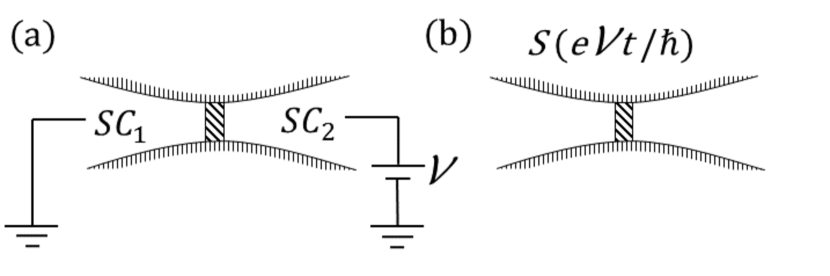
Figure 1: (a) A point contact between two superconductors SC₁ and SC₂ under applied bias $\mathcal{V}$. (b) To evaluate the dissipative current due to the quasiparticles at finite temperature $T$, we absorb the bias voltage in the time dependence of the quasiparticle scattering matrix $S(\Omega\,t)$, where $\Omega=e\mathcal{V}/\hbar$. The main general expression for dissipative conductance $G$ is given in Eq. (12) and application to a specific model of a superconducting point contact (SPC) in Eq. (15).

Aiming at evaluation of $G(T)$ for a system with broken gauge invariance, it is useful to reformulate the problem so that the chemical potentials of the leads are not affected by the bias. This is achieved by introducing a time-dependent phase $e{\cal V}t/\hbar$ in the definition of the creation operators for electrons to which bias is applied, $\psi^{\dagger}\rightarrow\psi^{\dagger}\exp(ie{\cal V}t/\hbar)$ and thus endowing the scattering matrix describing the contact with a periodic dependence on time, see Fig. 1. The time dependence allows for energy absorption by electrons passing through the junction, i.e., introduces channels of inelastic scattering. The energy transfer is quantized in units of $\hbar\Omega=e{\cal V}$, small in the limit ${\cal V}\to 0$. Our strategy consists of two steps. First, we relate the scattering matrix for such “soft” inelastic processes to the conventionally-defined elastic scattering matrix of the system in the absence of time dependence. Next, we evaluate the absorbed power ${\cal P}$ in terms of scattering matrix and find $G(T)$ from the relation ${\cal P}=G{\cal V}^{2}$ for Ohmic losses. This method avoids problems associated with the charge nonconservation and presence of large nondissipative currents. The result, Eq. (12), is applicable to superconducting and hybrid normal metal–superconductor structures. For such structures, Eq. (12) has the same status as that of the standard Landauer formula for the normal-state contacts; in the absence of superconductivity, Eq. (12) readily reduces to the conventional form of the Landauer formula.

Inelastic quasiparticle scattering in channel $N$ is associated with absorption of $N$ quanta ($N=0,\pm 1,\pm 2,\dots$) and is characterized by scattering matrix $S_{N}$. In order to relate $S_{N}$ to the elastic scattering matrix, we consider a generic scattering problem with a Hamiltonian

$$H =H_{0}+W(t),$$ (1)

$$W(t) =Ve^{-i\phi(t)}+V^{\dagger}e^{i\phi(t)}+V_{0},$$

where $H_{0}$ describes the two leads, and $W(t)$ represents the coupling between them ($V$ and $V^{\dagger}$ terms) and backscattering off the junction (term $V_{0}$) . In the case of the time-independent phase, $\phi(t)=\phi$, scattering is elastic and described by an instantaneous scattering matrix $S(\phi)$. At a finite bias, the phase $\phi(t)=\Omega\,t$ winds with frequency $\Omega$, allowing for inelastic transitions with energy transfer $N\hbar\Omega$.

To relate $S_{N}$ to $S(\phi)$, we compare their respective representations by infinite-order series in $W$. For that, we inspect the time evolution of the wave function $|{\psi(t)}\rangle=U(t)|{m}\rangle$ with the initial state $|m\rangle$ at $t=-\infty$; here $|m\rangle$ is an eigenstate of $H_{0}$ with energy $\varepsilon_{m}$. The evolution operator is given by the usual time-ordered exponential $U(t)=\mathcal{T}\exp\left[\frac{1}{i\,\hbar}\int_{-\infty}^{t}dt_{1}W_{I}(t_{1})\right]$, and the subscript $I$ stands for the interaction representation. The $k$-th order expansion term of the evolution operator Sitenko (1991) reads

$$U_{k}(t)=\frac{1}{(i\,\hbar)^{k}}\int_{-\infty}^{t}\!\!\!dt_{k}W_{I}(t_{k})\,\dots\int^{t_{2}}_{-\infty}\!\!\!dt_{1}W_{I}(t_{1}).$$

At this point, it is convenient to introduce a variable $s$ taking values $0,\pm 1$ and rewrite $W(t)=\sum_{s}V^{s}e^{is\phi(t)}$, where $V^{-1}\equiv V$, $V^{+1}\equiv V^{\dagger}$, and $V^{0}\equiv V_{0}$. That allows one to further specify the form of the expansion term. For $\phi(t)=\Omega\,t$, we may write $U_{k}(t)$ as a sum of harmonics,

$$U_{k}(t)=\sum_{N}\frac{e^{iN\Omega t}}{(i\,\hbar)^{k}}\sum_{s_{1},\dots s_{k}}\delta_{\sigma_{k},N}\int_{-\infty}^{t}\!\!\!dt_{k}e^{i\sigma_{k}\Omega(t_{k}-t)}V^{s_{k}}_{I}(t_{k})$$

$$\qquad\qquad\qquad\qquad\dots\int_{-\infty}^{t_{2}}dt_{1}e^{i\sigma_{1}\Omega(t_{1}-t_{2})}V^{s_{1}}_{I}(t_{1}),$$ (2)

with $\sigma_{k}=s_{k}+\ldots+s_{1}$. A similar result for the static problem, $\phi(t)=\phi$, is obtained from Eq. (2) by replacing the factor $e^{iN\Omega t}\to e^{iN\phi}$ and setting $\Omega=0$ in all the integrands.

This form of $U_{k}(t)$ allows a direct comparison of the perturbative expansion of the wave functions for linearly winding phase $\phi(t)=\Omega\,t$, and for fixed phase $\phi(t)=\phi$, which we denote $|{\tilde{\psi}(t)}\rangle$ and $|\psi(t)\rangle$, respectively. Projecting the two wave functions onto the energy eigenstate $|n\rangle$ of $H_{0}$ with energy $\varepsilon_{n}$, we find

$$\langle n|\tilde{\psi}(t)\rangle\equiv\langle n|\left[U(t)|_{\phi(t)=\Omega t}\right]|m\rangle$$ (3)

$$=\delta_{nm}+\sum_{N}\frac{1}{i\,\hbar}\int_{-\infty}^{t}dt^{\prime}\,e^{i(\varepsilon_{n,m}+\hbar\Omega N)t^{\prime}/\hbar-0|t^{\prime}|}\,\mathcal{\tilde{T}}_{nm}(N,\Omega)$$

and

$$\langle n|\psi(t)\rangle\equiv\langle n|\left[U(t)|_{\phi(t)=\phi}\right]|m\rangle$$ (4)

$$=\delta_{nm}+\frac{1}{i\,\hbar}\int_{-\infty}^{t}dt^{\prime}\,e^{i\varepsilon_{n,m}t^{\prime}/\hbar-0|t^{\prime}|}\,\mathcal{T}_{nm}(\phi)\,.$$

The ${\cal T}$-matrices introduced above are given by the following series:

$$\mathcal{\tilde{T}}_{nm}(N,\Omega)=\sum_{k=1}^{\infty}\sum_{\begin{subarray}{c}m_{k-1},\ldots,m_{1}\\ s_{k}+...+s_{1}=N\end{subarray}}$$ (5)

$$\qquad\times\frac{V^{s_{k}}_{nm_{k-1}}\ldots V^{s_{1}}_{m_{1}m}}{(\varepsilon_{m,m_{k-1}}-\hbar\Omega\,\sigma_{k-1}+i0)\ldots(\varepsilon_{m,m_{1}}-\hbar\Omega\,\sigma_{1}+i0)}$$

and

$$\mathcal{T}_{nm}(\phi)=$$ (6)

$$\sum_{N}e^{i\phi N}\sum_{k=1}^{\infty}\sum_{\begin{subarray}{c}m_{k-1},\ldots,m_{1}\\ s_{k}+...+s_{1}=N\end{subarray}}\frac{V^{s_{k}}_{nm_{k-1}}\ldots V^{s_{1}}_{m_{1}m}}{(\varepsilon_{m,m_{k-1}}+i0)\ldots(\varepsilon_{m,m_{1}}+i0)}.$$

Here, we introduced the notation $\varepsilon_{m,n}=\varepsilon_{m}-\varepsilon_{n}$ and wrote the matrix elements as $V^{s}_{mn}=\langle m|V^{s}|n\rangle$. A finite $\Omega$ brings about inelastic transitions with an arbitrary integer number $N$ of energy quanta $\hbar\Omega$ being released ($N>0$) or absorbed ($N<0$). The corresponding transition amplitudes are given by $\mathcal{\tilde{T}}_{nm}(N,\Omega)$. In the case of fixed-phase, $\phi(t)=\phi$, the scattering is elastic.

By comparing the inelastic (5) and elastic (6) ${\cal T}$-matrices, we note that in the limit $\Omega\to 0$

$$\mathcal{\tilde{T}}_{nm}(N,0)=\int_{0}^{2\pi}\,\frac{d\phi}{2\pi}\,\mathcal{T}_{nm}(\phi)\,e^{-i\phi N}.$$ (7)

The utility of this expression is that the scattering matrix of a time-independent problem may be easier to evaluate. The use of Eq. (7) is justified as long as the effect of $\hbar\Omega$ in the energy denominators of Eq. (5) is negligible. An applicability criterion specific to a superconducting junction is discussed at the end of the Letter. We note in passing that Eq. (7) agrees with the “frozen scattering matrix” principle set forward in Refs. [Moskalets and Büttiker, 2004,Arrachea and Moskalets, 2006]. Next, we evaluate dissipative conductance using Eq. (7).

The dissipated power may be written using scattering theory, where the absorbed power, averaged over states in equilibrium, is

$$\mathcal{P}=\frac{2\pi}{\hbar}\sum_{N}N\hbar\Omega\sum_{n,m}\left|\mathcal{\tilde{T}}_{nm}(N,\Omega)\right|^{2}$$ (8)

$$\quad\times\left[f(\varepsilon_{n})-f(\varepsilon_{m})\right]\,\delta(\varepsilon_{n}-\varepsilon_{m}+\hbar\Omega N).$$

Each term in the sum over $N$ here has a simple meaning: it is a product of the energy $N\hbar\Omega$ absorbed in a transition, multiplied by the transition rate (here $f(\varepsilon_{n,m})$ are fermionic occupation factors). In the framework of scattering theory, it is customary to work in the continuous energy representation instead of the discrete indices $n$ and $m$. Therefore, we replace $n\to(\varepsilon^{\prime}\alpha)$, $m\to(\varepsilon\beta)$ and introduce the density of states $\rho_{\alpha}(\varepsilon^{\prime})$ and $\rho_{\beta}(\varepsilon)$ to re-write Eq. (8) in the form

$$\mathcal{P} =\frac{2\pi\hbar\Omega}{\hbar}\sum_{N}N\,\sum_{\alpha,\beta}\iint d\varepsilon^{\prime}d\varepsilon\,\rho_{\alpha}(\varepsilon^{\prime})\rho_{\beta}(\varepsilon)$$ (9)

$$\times\left|\mathcal{\tilde{T}}_{\varepsilon^{\prime}\alpha\,,\,\varepsilon\beta}(N,\Omega)\right|^{2}\,\left[f(\varepsilon^{\prime})-f(\varepsilon)\right]\,\delta(\varepsilon^{\prime}-\varepsilon+\hbar\Omega N).$$

Here, $\alpha$ and $\beta$ are the residual discrete indices; they may label channels, leads, particle-hole branches, etc. We integrate Eq. (9) over $\varepsilon^{\prime}$ and expand to the lowest (second) order in $\Omega$

$$\mathcal{P} =\frac{2\pi(\hbar\Omega)^{2}}{\hbar}\sum_{N}N^{2}\,\sum_{\alpha\beta}\int d\varepsilon\,\rho_{\alpha}(\varepsilon)\rho_{\beta}(\varepsilon)$$ (10)

$$\qquad\qquad\times\left|\mathcal{\tilde{T}}_{\varepsilon\alpha\,,\,\varepsilon\beta}(N,0)\right|^{2}\,[-\partial_{\varepsilon}f(\varepsilon)].$$

Crucially, the inelastic ${\cal T}$-matrix $\tilde{\cal T}(N,\Omega=0)$ is evaluated at $\Omega=0$ in Eq. (10). So we may express it via the elastic ${\cal T}$-matrix according to Eq. (7),

$$\mathcal{P}=\frac{2\pi(\hbar\Omega)^{2}}{\hbar}\int d\varepsilon\,[-\partial_{\varepsilon}f(\varepsilon)]\iint\limits_{0}^{\quad 2\pi}\frac{d\phi^{\prime}d\phi}{(2\pi)^{2}}$$ (11)

$$\times\sum_{N}e^{iN(\phi^{\prime}-\phi)}N^{2}\,\sum_{\alpha\beta}\rho_{\alpha}(\varepsilon)\rho_{\beta}(\varepsilon)\,{\mathcal{T}}^{\ast}_{\varepsilon\alpha\,,\,\varepsilon\beta}(\phi^{\prime})\mathcal{T}_{\varepsilon\alpha\,,\,\varepsilon\beta}(\phi).$$

Next we use the relationSitenko (1991), between the ${\cal T}$-matrix and the on-shell elastic scattering matrix and replace the derivatives $-2\pi i\sqrt{\rho_{\alpha}(\varepsilon)\rho_{\beta}(\varepsilon)}\,\partial_{\phi}\mathcal{T}_{\varepsilon\alpha\,,\,\varepsilon\beta}(\phi)\to\partial_{\phi}S_{\alpha\beta}(\phi,\varepsilon)$, which allows one to express the summation over $\alpha$ and $\beta$ as a trace. Further simplification comes from noticing that $\sum_{N}e^{iN(\phi^{\prime}-\phi)}N^{2}=2\pi\partial_{\phi}\partial_{\phi^{\prime}}\delta(\phi-\phi^{\prime})$ in Eq. (11). Finally, recalling that $\Omega=\mathcal{V}e/\hbar$ and $G=\mathcal{P}/\mathcal{V}^{2}$, we obtain the dissipative conductance, which is the main result of this work:

$$G=\frac{e^{2}}{h}\int\limits d\varepsilon\,[-\partial_{\varepsilon}f(\varepsilon)]\int\limits_{0}^{2\pi}\frac{d\phi}{2\pi}\,{\rm Tr}\left\{\partial_{\phi}S^{\dagger}(\phi,\varepsilon)\,\partial_{\phi}S(\phi,\varepsilon)\right\}.$$ (12)

Consistently with Eq. (1), the gauge in Eq. (12) is fixed by associating the phase factor $e^{i\phi}$ with the transmission amplitude of the normal-state scattering matrix. For a superconducting junction, the order parameter phase difference across the junction is $\varphi=2\phi$.

It is instructive to relate the dc conductance $G$ to the dissipative part of the low-frequency admittance $Y(\omega\to 0,\phi,T)$ of the same junction.  In evaluating ${\rm Re}\,Y({\omega\to 0},\phi,T)$, the perturbation $\delta\phi(t)=eU\cos(\omega t)/\hbar\omega$ of the phase $\phi(t)=\phi+\delta\phi(t)$ across the junction is a small parameter, as the limit $U\to 0$ is taken first. Applying the same technique as above, we find that only single-quantum transitions occur to linear order in $U$, with amplitudes $\propto\partial_{\phi}S$ . Evaluation of the absorption power yields 

$${\rm Re}\,Y(\omega\to 0,\phi,T)$$ (13)

$$=\frac{e^{2}}{h}\int\limits d\varepsilon\,[-\partial_{\varepsilon}f(\varepsilon)]\,{\rm Tr}\left\{\partial_{\phi}S^{\dagger}(\phi,\varepsilon)\,\partial_{\phi}S(\phi,\varepsilon)\right\}.$$

Comparing Eq. (12) with (13) and recalling that the phase winds with time as $e{\cal V}t/\hbar$, we conclude that $G$ may be viewed as a time-averaged value

$$G=\overline{{\rm Re}\,Y(\omega\to 0,e{\cal V}t/\hbar,T)}$$ (14)

of the instantaneous conductance given by the dissipative part of the admittance. It generalizes the known relation in normal junctions Bruus and Flensberg (2004) between the dc Landauer conductance and the $\omega\to 0$ limit of the Kubo formula.

Equation (12) is non-perturbative in tunneling, which is one of its advantages over the known Tinkham (2004); Larkin and Ovchinnikov (1967) results. We illustrate the utility of Eq. (12) by finding the conductance between two superconductors connected by a short channel of arbitrary transmission coefficient, see Fig. 1. Finite temperature induces a thermal population of quasiparticles in each of the two leads. To start with, we focus on the case of equal gaps $\Delta_{1}=\Delta_{2}=\Delta$. We follow Ref. [Beenakker, 1991] and evaluate the corresponding $S$-matrix. In the Bogoliubov-de Gennes representation, the quasiparticle excitations have positive energy $\varepsilon>\Delta$, and the S-matrix is 4-by-4 due to the 2 leads and 2 particle-hole branches, see  [*[SeeAppendix][forfurtherdetails.]SM] for details. We apply Eq. (12) and evaluate the conductance at arbitrary transmission coefficient $\tau$ of the junction,

$$\frac{G_{SPC}}{G_{n}}=\int_{\Delta}^{\infty}d\varepsilon\,[-\partial_{\varepsilon}f(\varepsilon)]\,\frac{2\,\varepsilon^{2}}{\sqrt{(\varepsilon^{2}-\Delta^{2})(\varepsilon^{2}-\Delta^{2}(1-\tau))}}.$$ (15)

Here $G_{n}=2e^{2}\tau/h$ is the normal-state conductance. An alternative way to derive Eq. (15) is to use Eq. (14) and the result Kos et al. (2013) for ${\rm Re}\,Y(\Omega,\phi,T)$.

It is instructive to consider first the low-temperature asymptote, $\Delta/T\gg 1$,

$$\frac{G_{SPC}(\Delta/T,\tau)}{G_{n}(\tau)}$$ (16)

$$\qquad\approx\sqrt{\frac{2\Delta}{\Delta+\varepsilon_{A}(\tau)}}\,\frac{\Delta}{T}\,e^{-\frac{\Delta+\varepsilon_{A}(\tau)}{2\,T}}K_{0}\left[\frac{\Delta-\varepsilon_{A}(\tau)}{2T}\right],$$

where $K_{0}(x)$ is the modified Bessel function. Note that the superconducting contact supports Andreev levels with energies $\varepsilon_{A}(\tau,\phi)=\Delta\sqrt{1-\tau\sin^{2}\phi}$ carrying the Josephson current, which is not the subject of this work. However the indirect effect of the Andreev levels is observed in Eqs. (15) and (16), where we denote $\varepsilon_{A}(\tau)\equiv\varepsilon_{A}(\tau,\pi/2)=\Delta\sqrt{1-\tau}$. The Andreev levels lead to a strong modification of the density of states of the delocalized quasiparticles and thus influence their transport. The low-temperature conductance (16) displays a crossover between two asymptotes defined by a dimensionless ratio $\frac{\Delta-\varepsilon_{A}}{T}\propto\frac{\tau\Delta}{T}$. Above the crossover temperature ($T\gg\tau\Delta$), the conductance may be approximated as $G_{SPC}=G_{n}\frac{\Delta}{T}\ln[4\,e^{-\gamma}\,T/(\Delta-\varepsilon_{A})]e^{-\frac{\Delta}{T}}$ (here $\gamma$ is the Euler-Mascheroni constant). We note that the perturbative-in-$\tau$ resultLarkin and Ovchinnikov (1967); Tinkham (2004) which diverges as $2e{\cal V}\to 0$, is cut off by the scale $\Delta-\varepsilon_{A}$. Below the crossover temperature ($T\ll\tau\Delta$), one finds $G_{SPC}=G_{n}\sqrt{{\frac{2\pi\Delta}{\tau T}}}e^{-\frac{\Delta}{T}}$. Both asymptotes are illustrated in Fig. 2(a).

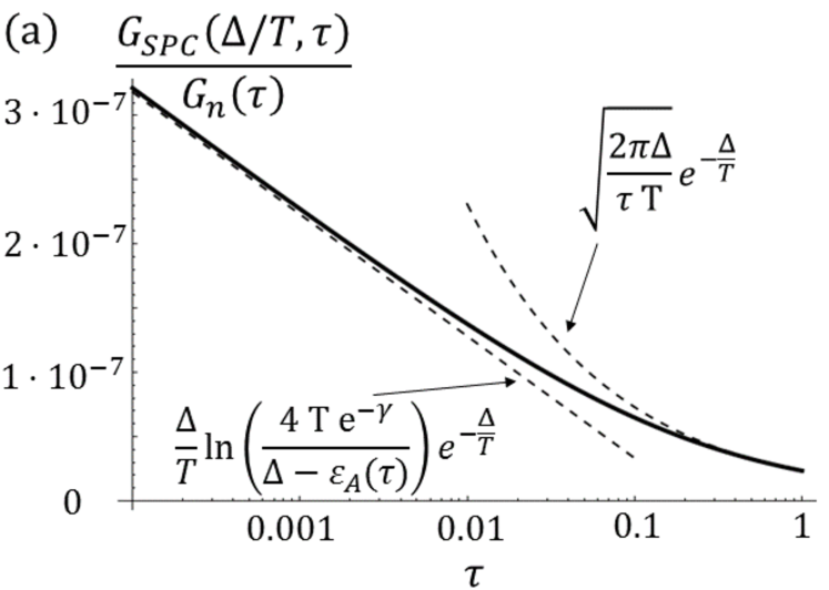
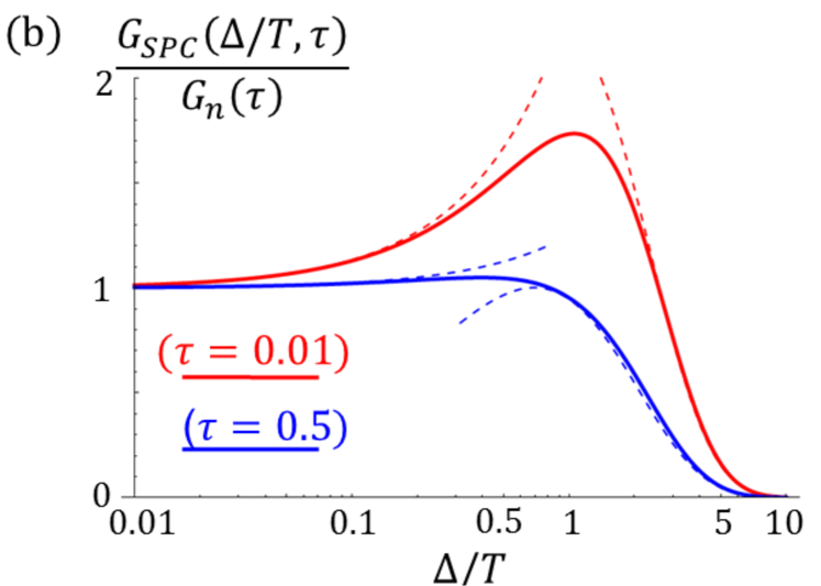
Figure 2: (a) Conductance $G_{SPC}$ of a superconducting point contact as a function of transmission coefficient $\tau$ evaluated from Eq. (15) at a low temperature, $T/\Delta=0.05$. The two asymptotes of Eq. (16), shown in dashed lines, are valid, respectively, at transmission $\tau\ll T/\Delta$ and $\tau\gg T/\Delta$. (b) $G_{SPC}$ as a function of $\Delta/T$ (solid lines) at two fixed values of $\tau$, along with the asymptotes (16) and (17), shown by dashed lines.

The high-temperature $T\gg\Delta$ (i.e. small-gap) asymptote is

$$\frac{G_{SPC}(\Delta/T,\tau)}{G_{n}(\tau)}\approx 1+\frac{\Delta}{T}\,k(\tau)\,.$$ (17)

Note that the coefficient $k(\tau)\geq 0$ (see Ref. [SM, ] for the full expression). It is logarithmically large, $k(\tau)\sim-\frac{1}{4}\ln\tau$, for $\tau\rightarrow 0$, and $k(\tau=1)=0$ . Therefore, at any $\tau<1$ the conductance $G_{SPC}$ initially grows with the opening of the superconducting gap $\Delta$. We plot the dependence of $G_{SPC}$ on $\Delta/T$ in Fig. 2(b) and observe that the conductance reaches maximum at $\Delta\sim T$. Note that the thermoelectric transport coefficients of SPC exhibit similar behaviorPershoguba and Glazman (2019).

The dissipative conductance Eq. (15) involves an unusual type of multiple Andreev reflection processes. In such events, quasiparticles are not created but rather gain energy exceeding $e{\cal V}$ at $N>1$. In the context of Eqs. (8)–(10), $N$ represents the number of energy quanta $\hbar\Omega$ absorbed or emitted during the quasiparticle tunneling. Because of the relation $\hbar\Omega=e\mathcal{V}$, integer $N$ also has the meaning of the number of electrons passing through the junction in a scattering event. The corresponding probabilities are given by the appropriately thermally-averagedSM values of $|\mathcal{\tilde{T}}(N,\Omega)|^{2}$, see Eq. (10). At $T\ll\Delta\cdot\tau$, the averaged $|\mathcal{\tilde{T}}(N,\Omega)|^{2}$ depend weakly on $N$ for $N<N^{\ast}=\sqrt{\Delta\tau/T}$ and decay as $\left|\tilde{T}(N,\Omega)\right|^{2}\sim 1/N^{4}$ for $N>N^{\ast}$. This indicates that processes with a transfer of a large number of electrons gain significance at low temperatures.

If both leads are superconducting, the series for the absorbed power (10) contains infinitely many terms in $N$, and the trace formula (12) is an agile way to calculate $G$. If at least one of the leads is non-superconducting, the sum over $N$ in Eq. (10) truncates. As an example, we consider an NS junction, i.e. set $\Delta_{1}=0$, $\Delta_{2}=\Delta$. It is easy to see SM that the highest harmonics of the elastic S-matrix are $e^{\pm 2i\phi}$, truncating the series at $|N|=2$. Evaluating the sum or using the trace formula (12), and accounting for the unitarity of the S-matrix, we recover the known Blonder et al. (1982) expression,

$$G_{NS}=\frac{2e^{2}}{h}\int_{0}^{\infty}d\varepsilon\,[ - \partial_{\varepsilon}f(\varepsilon)]\left[(1-|r^{ee}|^{2}+|r^{he}|^{2})\right.$$ (18)

$$+ (1-|r^{hh}|^{2}+\left.|r^{eh}|^{2})\right]\,,$$

where $r^{ee}(\varepsilon)$, $r^{hh}(\varepsilon)$, and $r^{he}(\varepsilon)$, $r^{eh}(\varepsilon)$ are, respectively, the particle, hole, and two Andreev reflection amplitudes . The S-matrix of a normal junction ($\Delta_{1}=\Delta_{2}=0$) contains only $e^{\pm i\phi}$ harmonics, along with a $\phi$-independent part. As a result, $r^{he}(\varepsilon)=r^{eh}(\varepsilon)=0$ and Eq. (18) reduces to the standard Landauer formula in the particle-hole representation.

In the derivation of Eq. (12), we relied upon the relation between elastic and “soft” inelastic scattering matrices, cf. Eq. (7). This is justified as long as $\hbar\Omega$ is negligible compared to the typical energy differences $\varepsilon_{m}-\varepsilon_{m^{\prime}}$ involved in the summation over virtual states. In the context of a tunnel junction between two superconductors with gaps $\Delta_{1}\neq\Delta_{2}$, one may estimate the significance of the next-order in $\Omega=e\mathcal{V}/\hbar$ terms by expanding in ${\cal V}$ the known Larkin and Ovchinnikov (1967) expression, $I(\mathcal{V})=I_{1}(\mathcal{V})+I_{3}(\mathcal{V})+\mathcal{O}(\mathcal{V}^{5})$, where $I_{n}(\mathcal{V})\propto\mathcal{V}^{n}$. We evaluate the ratio of the consecutive terms in the expansion of currentSM and find $\frac{I_{3}}{I_{1}}\propto\frac{(e\mathcal{V})^{2}}{T^{2}}$ and $\frac{I_{3}}{I_{1}}\propto\frac{(e\mathcal{V})^{2}}{(\Delta_{1}-\Delta_{2})^{2}}$ in the cases $|\Delta_{1}-\Delta_{2}|\gg T$ and $|\Delta_{1}-\Delta_{2}|\ll T$, respectively. In other words, the next-order corrections in $e\mathcal{V}$ may be dropped as long as $\hbar\Omega=e\mathcal{V}$ is the smallest energy scale in the problem. At finite transmission $\tau$ and equal gaps, for which Eq. (15) is derived, this applicability criterion amounts to $e\mathcal{V}\ll{\rm min}[\,T,\Delta-\varepsilon_{A}(\tau)]$.

It is worth emphasizing that the derived dissipative conductance $G_{SPC}$, Eq. (15), is entirely due to the itinerant Bogoliubov quasiparticles passing through the junction. The associated Andreev levels do not contribute to the dissipation in the absence of relaxation. The latter creates an additional channel of dissipation via the Debye mechanism Debye (1912). To quantify this, we introduce a phenomenological relaxation rate $\gamma$ for an occupied Andreev level Averin and Bardas (1996) and estimate the ratio $\frac{I_{A}}{I_{qp}}$ of the dissipative current $I_{A}(\mathcal{V})$ due to the Andreev levelsSM and the current $I_{qp}(\mathcal{V})=G_{SPC}\mathcal{V}$ due to the quasiparticles. In the limit $\frac{\tau\Delta}{T}\ll 1$, we estimate $\frac{I_{A}}{I_{qp}}\propto\frac{\tau}{\ln(T/\tau\Delta)}\frac{\Delta\,\hbar\gamma}{(\hbar\gamma)^{2}+(2e\mathcal{V})^{2}}$, indicating that the quasiparticle current $I_{qp}$ dominates even in the linear-in-${\cal V}$ regime ($e{\cal V}\ll\hbar\gamma$) provided the relaxation rate $\hbar\gamma\gtrsim\tau\Delta$. In the limit of low temperatures $T/\Delta\ll 1$ and intermediate $\tau$, we find that the ratio of currents scales as $\frac{I_{A}}{I_{qp}}\propto\frac{T}{\hbar\gamma}\exp[\frac{\Delta}{T}(1-\sqrt{1-\tau})]$ and $\frac{I_{A}}{I_{qp}}\propto\frac{T\,\hbar\gamma}{(e\mathcal{V})^{2}}\exp[\frac{\Delta}{T}(1-\sqrt{1-\tau})]$ in the opposite regimes of small ($e\mathcal{V}\ll\hbar\gamma$) and large ($e\mathcal{V}\gg\hbar\gamma$) bias, respectively. In the latter regime, the large exponential factor may be mitigated by a small $\gamma$. Note that in the absence of the relaxation due to phonons as, e.g., in the cold atom experiments Husmann et al. (2018), the relaxation is itself determined by the quasiparticle population and is, therefore, exponentially suppressed at low temperatures, $\gamma\propto\exp(-\Delta/T)$ .

In summary, we have expressed the dissipative linear conductance $G$ of a superconducting quantum point contact in terms of the scattering matrix for Bogoliubov quasiparticles, see Eq. (12). At a finite temperature, $G$ is finite; Eq. (12) adequately accounts for the thermally-excited quasiparticles passing through the junction. It generalizes the Landauer formula and is valid for junctions with normal or superconducting leads. In addition, we uncovered the relation (14) between the dc conductance and the phase-averaged real part of the ac admittance of a junction.

This work is supported by the DOE contract DE-FG02-08ER46482 (LIG), the ARO grant W911NF-18-1-0212 (SSP), and by the Yale Prize Postdoctoral Fellowship (TV).

Appendix A Elastic scattering matrix of a superconducting point contact at arbitrary $\Delta_{1}/\Delta_{2}$ .

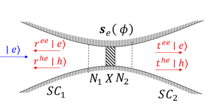
Figure 3: Bogoliubov-de Gennes model used to derive the scattering matrix of a single-channel superconducting point contact (SPC). The normal regions $N_{1}$ and $N_{2}$ are introduced for convenience of formulating a scattering problem. A typical scattering process is demonstrated with arrows: an incident particle-like quasiparticle (emphasized in blue) from the left superconductor scatters as particle-like or hole-like quasiparticles in both superconductors. The scattering matrix that describes such processes (26) is 4-by-4.

We consider a single-channel quantum contact shown in Fig. 3. In particle-hole representation, a typical scattering process of a Bogoliubov quasiparticle is demonstrated in colored arrows. A particle-like quasiparticle incident from the left superconductor is scattered in four channels (2 particle-hole and 2 leads) with the corresponding scattering amplitudes $r^{ee},r^{he},t^{ee}$, and $t^{he}$. It is convenient to collect all scattering amplitudes in a single 4-by-4 scattering matrix $[\psi^{-}_{e1},\psi^{+}_{e2},\psi^{-}_{h1},\psi^{+}_{h2}]^{\rm T}=\bm{S}(\phi,\varepsilon)\,[\psi^{+}_{e1},\psi^{-}_{e2},\psi^{+}_{h1},\psi^{-}_{h2}]^{\rm T}$ relating the incoming and outgoing states; here the superscript signs $\pm$ denote the direction of the group velocity. We follow Beenakker Beenakker (1991) and generalize the scattering matrix to the case of non-equal gaps $\Delta_{1}\neq\Delta_{2}$

$$\bm{S}(\phi,\varepsilon)=\bm{B}(\varepsilon)\left[\bm{I}-\bm{S}_{n}(\phi)\bm{A}(\varepsilon)]^{-1}\,\left[\bm{S}_{n}(\phi)-\bm{A}(\varepsilon)\right]\bm{B}^{-1}(\varepsilon),$$

$$\quad\bm{S}_{n}(\phi)=\left(\begin{array}[]{cc}\bm{s}_{e}(\phi)&\bm{0}\\ \bm{0}&\bm{s}_{h}(\phi)\end{array}\right),\quad\bm{A}(\varepsilon)=\left(\begin{array}[]{cc}\bm{0}&\bm{a}(\varepsilon)\\ \bm{a}(\varepsilon)&\bm{0}\end{array}\right),$$ (23)

$$\quad\bm{B}(\varepsilon)=\left(\begin{array}[]{cc}\sqrt{\bm{1}-\bm{a}^{2}(\varepsilon)}&\bm{0}\\ \bm{0}&\sqrt{\bm{1}-\bm{a}^{2}(\varepsilon)}\end{array}\right).$$ (26)

Within the Supplement, we choose a convention in which the bold upper-case (e.g. $\bm{S},\bm{S}_{n}$, $\bm{A}$, etc.) and lower-case (e.g. $\bm{s}_{e},\bm{s}_{h}$, $\bm{a}$, etc.) letters denote the 4-by-4 and 2-by-2 matrices, respectively. The matrix $\bm{S}_{n}$ describes the scatterer X in a normal state; its diagonal blocks $\bm{s}_{e}$ and $\bm{s}_{h}=\bm{s}_{e}^{\ast}$ act in the particle and hole subspaces. As stated after Eq. (12) of the main text, we absorb the phase $\phi$ into the off-diagonal elements of the scattering matrix

$$\bm{s}_{e}(\phi)=\left(\begin{array}[]{cc}r&i\,t\,e^{-i\phi}\\ i\,t\,e^{i\phi}&r\end{array}\right).$$ (29)

These matrix elements define the transmission amplitudes. This gauge is most convenient for the generalizations involving application of a voltage bias to the junction. Focusing on a short channel, we assume that the reflection $r$ and transmission $t$ amplitudes are energy independent. Note that the conventional Josephson phase difference $\varphi$ is related with the defined phase $\phi$ as $\varphi=2\phi$. The matrices

$$\bm{a}(\varepsilon)=\left(\begin{array}[]{cc}a_{1}(\varepsilon)&0\\ 0&a_{2}({\varepsilon})\end{array}\right),\quad a_{1,2}(\varepsilon)=\frac{\varepsilon-\sqrt{\varepsilon^{2}-\Delta^{2}_{1,2}}}{\Delta_{1,2}},$$ (32)

and $\bm{A}(\varepsilon)$ describe the Andreev reflection at the opposite ends of the channel, and matrix $\bm{B}(\varepsilon)$ describes the transmission at its boundaries. The form of $a_{1,2}(\varepsilon)$ in Eq. (32) allows for non-equal gaps $\Delta_{1}\neq\Delta_{2}$.

The scattering matrix (26) is valid at energies $\varepsilon\sim\Delta\ll E_{F}$.

Appendix B Conductance of a short channel connecting two superconductors with $\Delta_{1}=\Delta_{2}=\Delta$.

Below, we provide a detailed derivation of Eq. (15) for the dissipative conductance of a superconducting point contact (SPC), starting with Eq. (12) of the main text.

(i) In the case of equal gaps $\Delta_{1}=\Delta_{2}=\Delta$, the scattering matrix (26) becomes

$$\bm{S}=[\bm{I}-a\bm{S}_{n}\bm{\tau}_{x}]^{-1}[\bm{S}_{n}-a\bm{\tau}_{x}]$$ (33)

where $a=[\varepsilon-\sqrt{\varepsilon^{2}-\Delta^{2}}]/\Delta$, and we defined the 4-by-4 matrix

$$\bm{\tau}_{x}=\left(\begin{array}[]{cc}\bm{0}&\bm{1}\\ \bm{1}&\bm{0}\end{array}\right).$$

For brevity, we have dropped the arguments $\bm{\varepsilon}$ and $\phi$, but it is implied that $a\equiv a(\varepsilon)$ and $S_{n}\equiv S_{n}(\phi)$.

(ii) The scattering matrix (33) may be simplified to:

$$\bm{S}=-\frac{1}{a}\bm{\tau}_{x}+\frac{1-a^{2}}{a}[\bm{I}-a\bm{S}_{n}\bm{\tau}_{x}]^{-1}\bm{\tau}_{x}.$$ (34)

An evident consequence of Eq. (34) is that the scattering matrix simplifies, $\bm{S}=-\bm{\tau}_{x}$, at the gap edge, i.e. at $\varepsilon=\Delta$, where $a=1$. The $\phi$-dependence enters Eq. (34) only in the second term. Therefore, it is convenient to obtain the $\phi$-derivatives appearing in the trace of Eq. (12) of the main text as

$${\rm Tr}\left\{\partial_{\phi}\bm{S}^{\dagger}\,\partial_{\phi}\bm{S}\right\}$$

$$=\frac{(1-a^{2})^{2}}{a^{2}}{\rm Tr}\left\{\partial_{\phi}[\bm{I}-a\,\bm{\tau}_{x}\bm{S}_{n}^{\dagger}]^{-1}\,\partial_{\phi}[\bm{I}-a\,\bm{S}_{n}\bm{\tau}_{x}]^{-1}\right\},$$

where we permuted under the trace to eliminate additional $\bm{\tau}_{x}$ matrices and also used that $(\bm{X}^{\dagger})^{-1}=(\bm{X}^{-1})^{\dagger}$ for invertible matrices ${\bm{X}}$.

(iii) Using that $\partial\bm{X}^{-1}=-\bm{X}^{-1}\partial\bm{X}\bm{X}^{-1}$ for invertible matrices ${\bm{X}}$, we may evaluate the $\phi$-derivatives under the trace as follows:

$${\rm Tr}\left\{\partial_{\phi}\bm{S}^{\dagger}\,\partial_{\phi}\bm{S}\right\}$$

$$=\frac{(1-a^{2})^{2}}{a^{2}}\,{\rm Tr}\left\{[\bm{I}-a\,\bm{\tau}_{x}\bm{S}_{n}^{\dagger}]^{-1}[-\partial_{\phi}\,a\,\bm{\tau}_{x}\bm{S}_{n}^{\dagger}][\bm{I}-a\,\bm{\tau}_{x}\bm{S}_{n}^{\dagger}]^{-1}\right.$$

$$\qquad\qquad\left.\times[\bm{I}-a\,\bm{S}_{n}\bm{\tau}_{x}]^{-1}\,[-\partial_{\phi}\,a\,\bm{S}_{n}\bm{\tau}_{x}]\,[\bm{I}-a\,\bm{S}_{n}\bm{\tau}_{x}]^{-1}\right\}$$

$$=(1-a^{2})^{2}\,{\rm Tr}\left\{[(\bm{I}-a\,\bm{\tau}_{x}\bm{S}_{n}^{\dagger})(\bm{I}-a\,\bm{S}_{n}\bm{\tau}_{x})]^{-1}\,\bm{\tau}_{x}\,\partial_{\phi}\bm{S}_{n}^{\dagger}\,\right.$$

$$\qquad\qquad\left.\times[(\bm{I}-a\,\bm{S}_{n}\bm{\tau}_{x})(\bm{I}-a\,\bm{\tau}_{x}\bm{S}_{n}^{\dagger})]^{-1}\,\partial_{\phi}\bm{S}_{n}\,\bm{\tau}_{x}\,\right\}$$

$$=(1-a^{2})^{2}\,{\rm Tr}\left\{[\bm{I}(1+a^{2})-a\,(\bm{\tau}_{x}\bm{S}_{n}^{\dagger}+\bm{S}_{n}\bm{\tau}_{x})]^{-1}\,\bm{\tau}_{x}\,\partial_{\phi}\bm{S}_{n}^{\dagger}\,\right.$$

$$\qquad\qquad\left.\times[\bm{I}(1+a^{2})-a\,(\bm{\tau}_{x}\bm{S}_{n}^{\dagger}+\bm{S}_{n}\bm{\tau}_{x})]^{-1}\,\partial_{\phi}\bm{S}_{n}\,\bm{\tau}_{x}\,\right\},$$ (35)

where in the penultimate line we used $X^{-1}Y^{-1}=[YX]^{-1}$ and evaluated the corresponding products in Eq. (35).

(iv) It is possible to check that

$$[\bm{I}(1+a^{2})-a\,(\bm{\tau}_{x}\bm{S}_{n}^{\dagger}+\bm{S}_{n}\bm{\tau}_{x})]$$

$$\qquad\times[\bm{I}(1+a^{2})+a\,(\bm{\tau}_{x}\bm{S}_{n}^{\dagger}+\bm{S}_{n}\bm{\tau}_{x})]=D\,\bm{I},$$

by substituting the explicit expression for $\bm{S}_{n}$. Here $D=1+a^{4}-2a^{2}(r^{2}+t^{2}\cos 2\phi)$ is (an energy-dependent) scalar. Thus, the inverse matrices appearing in Eq. (35) may be written explicitly as

$$[\bm{I}(1+a^{2})-a\,(\bm{\tau}_{x}\bm{S}_{n}^{\dagger}+\bm{S}_{n}\bm{\tau}_{x})]^{-1}=$$

$$\qquad\frac{1}{D}[\bm{I}(1+a^{2})+a\,(\bm{\tau}_{x}\bm{S}_{n}^{\dagger}+\bm{S}_{n}\bm{\tau}_{x})].$$

Using this relation in Eq. (35), we obtain

$${\rm Tr}\left\{\partial_{\phi}\bm{S}^{\dagger}\,\partial_{\phi}\bm{S}\right\}$$

$$=\frac{(1-a^{2})^{2}}{D^{2}}\,{\rm Tr}\left\{[\bm{I}(1+a^{2})+a\,(\bm{\tau}_{x}\bm{S}_{n}^{\dagger}+\bm{S}_{n}\bm{\tau}_{x})]\,\bm{\tau}_{x}\,\partial_{\phi}\bm{S}_{n}^{\dagger}\,\right.$$

$$\qquad\qquad\qquad\left.\times[\bm{I}(1+a^{2})+a\,(\bm{\tau}_{x}\bm{S}_{n}^{\dagger}+\bm{S}_{n}\bm{\tau}_{x})]\,\partial_{\phi}\bm{S}_{n}\,\bm{\tau}_{x}\right\}.$$

(v) We expand the matrix appearing in the latter equation in powers of $\bm{\tau}_{x}$. Only the even-power terms contribute to the trace, so we may write

$${\rm Tr}\left\{\partial_{\phi}\bm{S}^{\dagger}\,\partial_{\phi}\bm{S}\right\}$$

$$=\frac{(1-a^{2})^{2}}{D^{2}}\,{\rm Tr}\left\{(1+a^{2})^{2}\,\bm{\tau}_{x}\,\partial_{\phi}\bm{S}_{n}^{\dagger}\,\partial_{\phi}\bm{S}_{n}\,\bm{\tau}_{x}\,\right.$$

$$\left.+a^{2}\,(\bm{\tau}_{x}\bm{S}_{n}^{\dagger}+\bm{S}_{n}\bm{\tau}_{x})\,\bm{\tau}_{x}\,\partial_{\phi}\bm{S}_{n}^{\dagger}\,(\bm{\tau}_{x}\bm{S}_{n}^{\dagger}+\bm{S}_{n}\bm{\tau}_{x})\,\partial_{\phi}\bm{S}_{n}\,\bm{\tau}_{x}\right\}.$$

By using the expression for $\bm{S}_{n}$ in terms of the matrices Eq. (29), the trace may be evaluated explicitly,

$${\rm Tr}\left\{\bm{\tau}_{x}\,\partial_{\phi}\bm{S}_{n}^{\dagger}\,\partial_{\phi}\bm{S}_{n}\,\bm{\tau}_{x}\,\right\}=4t^{2}$$

$${\rm Tr}\left\{(\bm{\tau}_{x}\bm{S}_{n}^{\dagger}+\bm{S}_{n}\bm{\tau}_{x})\,\bm{\tau}_{x}\,\partial_{\phi}\bm{S}_{n}^{\dagger}\,(\bm{\tau}_{x}\bm{S}_{n}^{\dagger}+\bm{S}_{n}\bm{\tau}_{x})\,\partial_{\phi}\bm{S}_{n}\,\bm{\tau}_{x}\,\right\}$$

$$\qquad=8t^{2}[t^{2}+(2-t^{2})\cos 2\phi].$$

Finally, collecting all terms together,we obtain:

$${\rm Tr}\left\{\partial_{\phi}\bm{S}^{\dagger}\,\partial_{\phi}\bm{S}\right\}$$

$$=\frac{4t^{2}(1-a^{2})^{2}\left[(1+a^{2})^{2}+2a^{2}t^{2}+2a^{2}(2-t^{2})\cos 2\phi\right]}{\left[(1-a^{2})^{2}+2a^{2}t^{2}(1-\cos 2\phi)\right]^{2}}.\,$$

(vi) Integration of the above expression over $\phi$ reproduces the integrand in Eq. (15) of the main text:

$$\int\frac{d\phi}{2\pi}\,{\rm Tr}\left\{\partial_{\phi}\bm{S}^{\dagger}\,\partial_{\phi}\bm{S}\right\}$$

$$\qquad=\frac{4t^{2}(1+a^{2})^{2}}{(1-a^{2})\sqrt{(1-a^{2})^{2}+4a^{2}t^{2}}}$$

$$\qquad=\frac{4t^{2}\varepsilon^{2}}{\sqrt{(\varepsilon^{2}-\Delta^{2})(\varepsilon^{2}-\Delta^{2}(1-t^{2}))}}.$$

Appendix C Conductance of the NS junction ($\Delta_{1}=0$, $\Delta_{2}=\Delta$).

Below, we provide details of derivation of the conductance of NS junction. Our goal here is to show how the known results Blonder et al. (1982) come out from Eq. (12) of the main text.

(i) We consider the case where the left lead is normal, i.e. $\Delta_{1}=0$, whereas the right lead is superconducting, i.e. $\Delta_{2}=\Delta$. This induces the following Andreev scattering amplitudes $a_{1}=0$ and $a_{2}=(\varepsilon-\sqrt{\varepsilon^{2}-\Delta^{2}})/\Delta\equiv a$. We also introduce $b=\sqrt{1-a^{2}}$, which has a meaning of transmission amplitude through a clean NS boundary. Plugging them in Eq. (26), one may obtain the 4-by-4 scattering matrix

$$\bm{S}\equiv\left(\begin{array}[]{cccc}r^{ee}_{11}&t^{ee}_{12}&r^{eh}_{11}&t^{eh}_{12}\\ t^{ee}_{21}&r^{ee}_{22}&t^{eh}_{21}&r^{eh}_{22}\\ r^{he}_{11}&t^{he}_{12}&r^{hh}_{11}&t^{hh}_{12}\\ t^{he}_{21}&r^{he}_{22}&t^{hh}_{21}&r^{hh}_{22}\end{array}\right)$$ (40)

$$=\frac{1}{D}\left(\begin{array}[]{cccc}b^{2}r&ibt\,e^{-i\phi}&at^{2}\,e^{-2i\phi}&iabrt\,e^{-i\phi}\\ ibt\,e^{i\phi}&b^{2}r&-iabrt\,e^{-i\phi}&-at^{2}\\ at^{2}\,e^{2i\phi}&-iabrt\,e^{i\phi}&b^{2}r&-ibt\,e^{i\phi}\\ iabrt\,e^{i\phi}&-at^{2}&-ibt\,e^{-i\phi}&b^{2}r\end{array}\right),$$ (45)

where $D=1-a^{2}r^{2}$. In the first line of Eq. (40), we gave an explicit representation of the matrix elements of the scattering matrix in terms of the scattering amplitudes, i.e. $t^{ee}_{21},\,t^{he}_{21}$, etc. Here the top indices label the particle-hole branches, whereas the bottom indices label the leads. For example, $t^{he}_{21}$ represents a process of a particle-like quasiparticle incident from the left (1) lead which scattering into a hole-like state in the right (2) lead.

(ii) Quasiparticles with low energies $\varepsilon<\Delta$. Consideration of the contribution to $G$ of the excitations with energy $\varepsilon<\Delta$ impinging on the interface from the normal lead is especially simple and insightful. In this case, the function $a(\varepsilon)$ becomes complex, $a(\varepsilon)=(\varepsilon-i\sqrt{\Delta^{2}-\varepsilon^{2}})/\Delta$. At energies $\varepsilon<\Delta$ excitations reside only in the left (normal) lead, so that the scattering matrix (40) reduces to 2-by-2

$$\bm{S}\equiv\left(\begin{array}[]{cc}r^{ee}_{11}&r^{eh}_{11}\\ r^{he}_{11}&r^{hh}_{11}\end{array}\right)=\frac{1}{1-a^{2}r^{2}}\left(\begin{array}[]{cc}b^{2}r&at^{2}\,e^{-2i\phi}\\ at^{2}\,e^{2i\phi}&b^{2}r\end{array}\right).$$ (50)

The only $\phi$-dependence here comes from Andreev reflection processes encoded in the exponential prefactors $\propto e^{2i\phi}$ of the off-diagonal elements. Using Eq. (50) it is straightforward to evaluate the $\phi$-integral in Eq. (12):

$$\int\limits_{0}^{2\pi}\frac{d\phi}{2\pi}\,{\rm Tr}\left\{\partial_{\phi}\bm{S}^{\dagger}(\phi,\varepsilon)\,\partial_{\phi}\bm{S}(\phi,\varepsilon)\right\}=4|r^{eh}_{11}|^{2}+4|r^{he}_{11}|^{2}.$$

Unitarity of the S-matrix allows us to re-write the latter equation as

$$\int\limits_{0}^{2\pi}\frac{d\phi}{2\pi}\,{\rm Tr}\left\{\partial_{\phi}\bm{S}^{\dagger}(\phi,\varepsilon)\,\partial_{\phi}\bm{S}(\phi,\varepsilon)\right\}$$

$$\qquad=2(1-|r^{ee}_{11}|^{2}+|r^{eh}_{11}|^{2})+2(1-|r^{hh}_{11}|^{2}+|r^{he}_{11}|^{2}).$$ (51)

(iii) Quasiparticles with energies $\varepsilon>\Delta$. Here the full 4-by-4 matrix (40) must be considered. In addition to the Andreev processes, it also contains single-particle transmission amplitudes decorated by factors $e^{i\phi}$. Evaluation of the proper trace is straightforward,

$$\int\limits_{0}^{2\pi}\frac{d\phi}{2\pi}\,{\rm Tr}\left\{\partial_{\phi}\bm{S}^{\dagger}(\phi,\varepsilon)\,\partial_{\phi}\bm{S}(\phi,\varepsilon)\right\}$$

$$\qquad=(4|r^{he}_{11}|^{2}+|t^{ee}_{21}|^{2}+|t^{he}_{21}|^{2}+|t^{ee}_{12}|^{2}+|t^{he}_{12}|^{2})$$

$$\qquad\qquad+(4|r^{eh}_{11}|^{2}+|t^{hh}_{21}|^{2}+|t^{eh}_{21}|^{2}+|t^{hh}_{12}|^{2}+|t^{eh}_{12}|^{2}).$$

Noting that $|t^{bb^{\prime}}_{12}|=|t^{bb^{\prime}}_{21}|$ for each quasiparticle branch and using the unitarity of the scattering matrix, it can be further simplified,

$$\int\limits_{0}^{2\pi}\frac{d\phi}{2\pi}\,{\rm Tr}\left\{\partial_{\phi}\bm{S}^{\dagger}(\phi,\varepsilon)\,\partial_{\phi}\bm{S}(\phi,\varepsilon)\right\}$$

$$\qquad=2(1-|r^{ee}_{11}|^{2}+|r^{eh}_{11}|^{2})+2(1-|r^{hh}_{11}|^{2}+|r^{he}_{11}|^{2}).$$ (52)

(iv) Given the identical form of Eqs. (51) and (52), we may write the conductance using Eq. (12) as

$$G_{NS}=\frac{2e^{2}}{h}\int_{0}^{\infty}d\varepsilon\,[ - \partial_{\varepsilon}f(\varepsilon)]\left[(1-|r^{ee}|^{2}+|r^{he}|^{2})\right.$$ (53)

$$+ (1-|r^{hh}|^{2}+\left.|r^{eh}|^{2})\right]\,.$$

The terms in the first and second parentheses represent, respectively, the particle-like and hole-like contributions to the conductance. Equation (53) agrees with the well-known expression for NS junctions Blonder et al. (1982). The concrete expression in terms of the transmission coefficient $\tau$ may also be evaluated after some algebra

$$\frac{G_{NS}}{G_{n}} =\int_{0}^{\Delta}d\varepsilon\,\frac{4\tau\Delta^{2}}{\Delta^{2}(2-\tau)^{2}-4\varepsilon^{2}(1-\tau)}[-\partial_{\varepsilon}f(\varepsilon)]$$

$$+\int_{\Delta}^{\infty}d\varepsilon\,\frac{4\,\varepsilon}{\tau\varepsilon+(2-\tau)\sqrt{\varepsilon^{2}-\Delta^{2}}}[-\partial_{\varepsilon}f(\varepsilon)].$$ (54)

Appendix D Asymptotic behavior of the superconducting point contact conductance at low $T\ll\Delta$ and high $T\gg\Delta$ temperatures.

Below, we provide details of finding asymptotic behavior of the formula for SPC conductance, with reference to Eq. (15) of the main text. It is convenient to switch there to a dimensionless integration variable $x$ defined as $\varepsilon/T=x$, so that integral becomes

$$\frac{G_{SPC}}{G_{n}}=\int_{\alpha}^{\infty}dx\,\frac{2\,x^{2}}{\sqrt{(x^{2}-\alpha^{2})(x^{2}-\alpha^{2}(1-\tau))}}[-f^{\prime}(x)],$$ (55)

where $\alpha=\Delta/T$ and $f(x)=(e^{x}+1)^{-1}$.

(i) Low temperature ($\alpha\gg 1$) asymptote. Here the Fermi function may be approximated with the Boltzmann distribution, $f(x)\approx e^{-x}$. It is convenient to further shift the integration variable, $x\to x+\alpha$,

$$\frac{G_{SPC}}{G_{n}}\approx$$

$$\int_{0}^{\infty}dx\,\frac{2\,(x+\alpha)^{2}}{\sqrt{[(x+\alpha)^{2}-\alpha^{2}][(x+\alpha)^{2}-\alpha^{2}(1-\tau)]}}e^{-x-\alpha}.$$

The terms $x$ can be neglected with respect to large $\alpha$ in the appropriate places of the integrand, which renders

$$\frac{G_{SPC}}{G_{n}}\approx$$

$$\alpha\sqrt{\frac{2}{1+\sqrt{1-\tau}}}\,e^{-\alpha}\int_{0}^{\infty}dx\,\frac{e^{-x}}{\sqrt{x[x+\alpha(1-\sqrt{1-\tau})]}}.$$

The integral may be recognized as the Bessel function $K_{0}(\lambda)=\int_{1}^{\infty}dx\,\frac{e^{-x\lambda}}{\sqrt{x^{2}-1}}$, and, thus, the conductance becomes

$$\frac{G_{SPC}}{G_{n}}\approx\alpha\,\sqrt{\frac{2}{1+\sqrt{1-\tau}}}\,e^{-\frac{\alpha}{2}(1+\sqrt{1-\tau})}\,K_{0}\left[\frac{\alpha}{2}(1-\sqrt{1-\tau})\right].$$

The asymptotes of the Bessel function here are $K_{0}(\lambda)\approx\sqrt{\frac{\pi}{2\lambda}}\,e^{-\lambda}$ for $\lambda\gg 1$ and $K_{0}(\lambda)\approx\ln\left(\frac{2e^{-\gamma}}{\lambda}\right)$ for $\lambda\ll 1$.

High-temperature ($\alpha\ll 1$) asymptote. In this limit, it is convenient to single out the trivial term in Eq. (55),

$$\frac{G_{SPC}}{G_{n}}=2\int_{\alpha}^{\infty}dx\,[-f^{\prime}(x)]+2\int_{\alpha}^{\infty}dx\,\left[\frac{x^{2}}{\sqrt{(x^{2}-\alpha^{2})(x^{2}-\alpha^{2}(1-\tau))}}-1\right][-f^{\prime}(x)],$$

at the expense of introducing $-1$ in the integrand of the second integral. The first integral is evaluated yielding $2f(\alpha)$. In the second integral, we bring the terms in the square brackets to the same denominator, multiply the numerator and denominator of the resulting fraction by the conjugate expression, and further switch to a new integration variable $x\to\alpha x$. Thus, we obtain

$$\frac{G_{SPC}}{G_{n}}=2f(\alpha)+2\alpha\int_{1}^{\infty}dx\,\left[\frac{(x^{2}-1)(2-\tau)+1}{\sqrt{(x^{2}-1)(x^{2}-1+\tau)}(x^{2}+\sqrt{(x^{2}-1)(x^{2}-1+\tau)})}\right][-f^{\prime}(\alpha x)],$$

Note that the expression in the square brackets of the integrand behaves as $1/x^{2}$ at large $x$, so the integral converges well. Thus, one may replace $-f^{\prime}(\alpha x)\approx 1/4$ to the leading order at small $\alpha$. That together with an expansion $f(\alpha)=1/2-\alpha/4$ gives an asymptotic approximation of the conductance at $\alpha=\Delta/T\ll 1$

$$\frac{G_{SPC}}{G_{n}}\approx 1+\alpha\,k(\tau),$$ (56)

where we introduced a $\tau$-dependent function

$$k(\tau)=-\frac{1}{2}+\frac{1}{2}\int_{1}^{\infty}dx\,\frac{(x^{2}-1)(2-\tau)+1}{\sqrt{(x^{2}-1)(x^{2}-1+\tau)}(x^{2}+\sqrt{(x^{2}-1)(x^{2}-1+\tau)})}.$$ (57)

The function $k(\tau)$ is positive on the interval $1>\tau>0$; it is logarithmically large $k(\tau)\approx-\frac{1}{4}\ln(\tau)$ at small $\tau\ll 1$ and vanishes $k(1)=0$ at perfect transmission $\tau=1$.

Appendix E Analysis of the series in $N$ in Eq. (10).

In the main part of the Letter, we obtained a representation of the absorbed power $\mathcal{P}$ via a series in $N$, see Eq. (10) of the main text. The integer $N$ stands for the number of absorbed/released energy quanta. The purpose of this section is to analyze the convergence of that series in $N$.

(i) For definiteness, we focus on a specific matrix element of the elastic scattering matrix $t^{he}(\phi)$ of a short channel connecting two superconducting leads. It has a simple form, Pershoguba and Glazman (2019)

$$t^{he}(\phi)=-r\frac{\xi}{t\Delta}\,\frac{\sin\phi}{(\xi/t\Delta)^{2}+\sin^{2}\phi},$$

where $\xi=\sqrt{\varepsilon^{2}-\Delta^{2}}$. The scattering amplitude $t^{he}(\phi)$ contributes to transport even in the tunnelling ($t\ll 1$) regime. Analysis of other amplitudes can be performed in a similar way.

(ii) The function $t^{he}(\phi)$ is periodic in $\phi$ and has only odd harmonics $t^{he}(\phi)=\sum_{N}\widetilde{t^{he}}(N)e^{i\phi N}$, where $N=2n+1$. One may evaluate them:

$$\widetilde{t^{he}}(N)=-\frac{r}{2i}\frac{\xi}{t\Delta}\frac{1}{\sqrt{1+\left(\frac{\xi}{t\Delta}\right)^{2}}\left[\left(\frac{\xi}{t\Delta}\right)+\sqrt{1+\left(\frac{\xi}{t\Delta}\right)^{2}}\right]^{N}}.$$ (58)

Recall that this Fourier harmonic also corresponds to the scattering amplitude with absorption of $N$ photons according to Eq. (7) of the main text.

(iii) Next, we seek to average the probability of that process over energy in the Gibbs ensemble,

$$P_{N}=\int_{\Delta}^{\infty}d\varepsilon\,\left|\widetilde{t^{he}}(N)\right|^{2}[-\partial_{\varepsilon}f(\varepsilon)].$$

To be specific, it corresponds to the integral $(2\pi)^{2}\int d\varepsilon\,\rho_{1}(\varepsilon)\rho_{2}(\varepsilon)\left|\mathcal{\tilde{T}}_{1\varepsilon\,\,2\varepsilon}(N,0)\right|^{2}\,[-\partial_{\varepsilon}f(\varepsilon)]$ in the notations of Eq. (10). For simplicity, we focus on a case of low temperatures $T\ll\Delta$, where the Fermi function simplifies $[-\partial_{\varepsilon}f(\varepsilon)]=\frac{1}{T}e^{-\varepsilon/T}$. In addition, one may expand $\varepsilon\approx\Delta+\xi^{2}/2\Delta$ and switch to the integration variable $\xi$. So, the integral becomes

$$P_{N}=\frac{1}{T}e^{-\Delta/T}\int_{0}^{\infty}d\xi\,\frac{\xi}{\Delta}\,|\widetilde{t^{he}}(N)|^{2}\,e^{-\xi^{2}/2\Delta T}.$$

Note that $\xi\sim t\Delta$ is an effective energy scale at which $\widetilde{t_{he}}(N)$ changes, whereas the exponential term in the integrand changes at the scale $\xi\sim\sqrt{\Delta T}$. In order to compare the two scales, it is instructive to switch to a dimensionless integration variable $x=\xi/t\Delta$. So, we substitute Eq. (58) in the last equation and obtain

$$P_{N}= \frac{\tau(1-\tau)\Delta}{T}\,e^{-\Delta/T}\,$$

$$\quad\times\int_{0}^{\infty}dx\,x^{3}\frac{e^{-x^{2}\Delta\tau/2T}}{(1+x^{2})(x+\sqrt{1+x^{2}})^{2N}},$$ (59)

where $\tau=t^{2}$.

(iv) Limit of small $\tau\Delta/T\ll 1$. In this limit, the exponential factor $e^{-x^{2}\Delta\tau/2T}$ may be neglected for $N>1$ because the integrand $\propto 1/x^{2N-1}$ converges well at $N>1$. In order to estimate the behavior of $P_{N}$ at large $N$, we notice that small $x\ll 1$ contribute most to the integral, so one may approximate the denominator of the integrand as $(1+x^{2})(x+\sqrt{1+x^{2}})^{2N}\approx(1+x)^{2N}\approx e^{2xN}$. It is, then, straightforward to find the asymptotics $P_{N}\propto 1/N^{4}$ at large $N$.

However at $N=1$, it is crucial to retain the exponential term $e^{-x^{2}\Delta\tau/2T}$, which cuts off the logarithmic divergence and produces $\propto\ln(T/\Delta\tau)$ after integration. It is interesting to note that it is the processes with the absorption or release of $N=1$ energy quanta that contribute most to transport at small $\tau$.

(iv) Limit of large $\tau\Delta/T\gg 1$. Because the integral converges at small $x$, we may also approximate the denominator $(1+x^{2})(x+\sqrt{1+x^{2}})^{2N}\approx e^{2xN}$. So, one may rewrite the integral in Eq. (59),

$$P_{N}\propto\int_{0}^{\infty}dx\,x^{3}\,e^{-2Nx}\,e^{-x^{2}\Delta\tau/2T}.$$

The competition of the two exponential factors determines the evolution of $P_{N}$ with $N$. For $N\ll N^{\ast}\sim\sqrt{\tau\Delta/T}$, the last exponential term dominates, so the integral depends weakly on $N$ producing a plateau in $P_{N}$. For $N\gg N^{\ast}\sim\sqrt{\tau\Delta/T}$, the first exponential term dominates, producing $P_{N}\propto 1/N^{4}$.

We conclude that the processes with the absorption of a large number of energy quanta (up to $N^{\ast}\sim\sqrt{\tau\Delta/T}$) are important at any $\tau$, as long as the condition $\tau\Delta/T\gg 1$ is satisfied.

Appendix F Expansion of $I(\mathcal{V})$ in powers of $\mathcal{V}$ in the tunnelling limit.

In the tunnelling limit $\tau\ll 1$, the full $I(\mathcal{V})$ dependence is known, Larkin and Ovchinnikov (1967); Tinkham (2004)

$$I(\mathcal{V})= \frac{G_{n}}{e}\int_{\Delta_{2}}^{\infty}d\varepsilon\,\left\{\rho_{1}(\varepsilon+e\mathcal{V})\,\rho_{2}(\varepsilon)\left[f(\varepsilon)-f(\varepsilon+e\mathcal{V})\right]\right.$$

$$\qquad\,\,\left.-\rho_{1}(\varepsilon-e\mathcal{V})\,\rho_{2}(\varepsilon)\left[f(\varepsilon)-f(\varepsilon-e\mathcal{V})\right]\right\}.$$ (60)

Here $\rho_{1,2}(\varepsilon)=\varepsilon/\sqrt{\varepsilon^{2}-\Delta_{1,2}^{2}}$ are the normalized densities of states in the two superconducting leads. For concreteness, we assume that the gaps are not equal and $\Delta_{2}>\Delta_{1}$. Current is an odd function of $\mathcal{V}$, so expansion of $I$ in $\mathcal{V}$ has only odd terms, $I(\mathcal{V})=I_{1}(\mathcal{V})+I_{3}(\mathcal{V})+\mathcal{O}(\mathcal{V}^{5})$ with $I_{n}\propto\mathcal{V}^{n}$. We find them by expanding (60) in ${\cal V}$,

$$I_{1}(\mathcal{V})=-2G_{n}\mathcal{V}\int^{\infty}_{\Delta_{2}}d\varepsilon\,\rho_{1}(\varepsilon)\rho_{2}(\varepsilon)\,\partial_{\varepsilon}f(\varepsilon),$$ (61)

$$I_{3}(\mathcal{V})=-2G_{n}e^{2}\mathcal{V}^{3}\,\int_{\Delta_{2}}^{\infty}d\varepsilon\,\rho_{2}(\varepsilon)\left[\frac{\rho_{1}(\varepsilon)\,\partial^{3}_{\varepsilon}f(\varepsilon)}{3!}\right.$$

$$\qquad\qquad\left.+\frac{\partial_{\varepsilon}\rho_{1}(\varepsilon)\,\partial^{2}_{\varepsilon}f(\varepsilon)}{2}+\frac{\partial^{2}_{\varepsilon}\rho_{1}(\varepsilon)\,\partial_{\varepsilon}f(\varepsilon)}{2}\right].$$ (62)

In order to compare the relative importance of the linear $I_{1}(\mathcal{V})$ and non-linear $I_{3}(\mathcal{V})$ currents we evaluate them in the limit of small temperatures $T\ll\Delta_{1}\sim\Delta_{2}$. We find that the ratio of the currents scales as $\frac{I_{3}}{I_{1}}\propto\left(\frac{e\mathcal{V}}{T}\right)^{2}$ and $\frac{I_{3}}{I_{1}}\propto\left(\frac{e\mathcal{V}}{\Delta_{2}-\Delta_{1}}\right)^{2}\frac{1}{\ln[T/(\Delta_{2}-\Delta_{1})]}$ in the regimes $T\ll(\Delta_{2}-\Delta_{1})$ and $T\gg(\Delta_{2}-\Delta_{1})$, respectively. This allows us to conclude that the non-linear term $I_{3}$ may be neglected as long as $e\mathcal{V}\ll\min(T,|\Delta_{2}-\Delta_{1}|)$ is the smallest energy scale.

Appendix G Dissipative current carried by the Andreev levels in the presence of relaxation.

(i) A short SPC supports Andreev levels with energies $\pm\varepsilon_{A}(\phi)$, where $\varepsilon_{A}(\phi)=\Delta\sqrt{1-\tau\sin\phi^{2}}$. Note the conventionally-defined Josephson phase difference is $\varphi=2\phi$. At thermodynamic equilibrium, the electric current carried by the Andreev levels is given by the Josephson relation

$$I_{A}(\phi)=-\frac{e}{\hbar}\,\partial_{\phi}\varepsilon_{A}(\phi)\,n_{eq}[\varepsilon_{A}(\phi)],$$ (63)

where $n_{eq}[\varepsilon_{A}]=f[-\varepsilon_{A}]-f[\varepsilon_{A}]=\tanh[\varepsilon_{A}/2T]$ is the difference of the fermionic occupations of the Andreev levels with negative $-\varepsilon_{A}$ and positive $\varepsilon_{A}$ energies.

(ii) Under the applied voltage bias $\mathcal{V}$, the phase winds, $\phi(t)=\Omega\,t$, with frequency $\Omega=e\mathcal{V}/\hbar$. This results in an ac Josephson effect, where the Josephson current $I_{A}(\phi(t))$ oscillates with frequency $2\,\Omega$. If averaged over the period of oscillations, the net current vanishes. However, relaxation may result in the non-zero net current due to the Debye mechanism Debye (1912). In order to describe it, we follow Ref. [Averin and Bardas, 1996] and introduce a phenomenological relaxation rate $\gamma$ of the occupation function

$$\frac{dn}{dt}+\gamma\,n=\gamma\,n_{eq}[\varepsilon_{A}(\phi(t))].$$ (64)

(iii) The solution of this equation may be presented in a general form

$$n(t)=\gamma\int_{-\infty}^{t}dt^{\prime}\,e^{-\gamma(t-t^{\prime})}\,n_{eq}[\varepsilon_{A}(\phi(t^{\prime}))].$$ (65)

This allows us to write the current $I_{A}(t)=-\frac{e}{\hbar}\,\partial_{\phi}\varepsilon_{A}(\phi(t))\,n(t)$ and average it over the period of oscillations

$$\langle I_{A}\rangle=\frac{\Omega}{\pi}\,\int_{0}^{\frac{\pi}{\Omega}}\,dt\,I_{A}(t)=-\frac{\Omega\,e}{\pi\,\hbar}\int_{0}^{\frac{\pi}{\Omega}}\,dt\,\partial_{\phi}\varepsilon_{A}(\phi(t))$$

$$\qquad\times\gamma\int_{-\infty}^{t}dt^{\prime}\,e^{-\gamma(t-t^{\prime})}\,n_{eq}[\varepsilon_{A}(\phi(t^{\prime}))].$$

We change integration variables $t\to\phi/\Omega$ and $t^{\prime}\to(\phi-\phi^{\prime})/\Omega$, exchange the order of integration, and further massage it to the form

$$\langle I_{A}\rangle=$$ (66)

$$-\frac{e}{\pi\hbar}\frac{\gamma}{\Omega}\,\int_{0}^{\infty}\,d\phi^{\prime}\,e^{-\frac{\gamma}{\Omega}\phi^{\prime}}\int_{0}^{\pi}\,d\phi\,\,\partial_{\phi}\,\varepsilon_{A}(\phi+\phi^{\prime})\,n_{eq}[\varepsilon_{A}(\phi)].$$

(iv) Limit of small $\tau$, such that $\frac{\tau\Delta}{T}\ll 1$. Then, the energy of the Andreev level can be approximated as $\varepsilon_{A}(\phi)\approx\Delta-\frac{\Delta\tau}{2}\sin^{2}\phi$, so $n_{eq}[\varepsilon_{A}(\phi)]\approx n_{eq}[\Delta]-\frac{\tau\Delta}{2}\sin^{2}\phi\,\,\partial_{\varepsilon}n_{eq}[\Delta]$. We plug these expansions in Eq. (66) and obtain

$$\langle I_{A}\rangle=\frac{e}{\hbar}\,\frac{\tau^{2}\Delta^{2}}{8}\,\frac{\gamma\,\Omega}{\gamma^{2}+4\Omega^{2}}\,\partial_{\varepsilon}n_{eq}[\Delta],$$

where recall that $\Omega=e\mathcal{V}/\hbar$.

(v) Limit of low temperatures $T/\Delta\ll 1$ and intermediate $\tau$ (i.e. $\tau\sim 1-\tau$). The main contribution to the dissipation comes from the vicinity of $\phi=\pi/2$ where the energy of Andreev level reaches minimum, and at low temperatures ($\Delta\sqrt{1-\tau}/T\gg 1$) the occupation factor can be approximated as

$$n[\varepsilon_{A}(\phi)]\approx$$

$$\,\,1-2\,\exp\left[-\frac{\Delta}{T}\sqrt{1-\tau}-\frac{\Delta}{T}\frac{\tau}{2\sqrt{1-\tau}}(\phi-\pi/2)^{2}\right].$$

Because of the large factor $\Delta/T$ in the exponent, the integral over $\phi$ in Eq. (66) converges fast. After performing integration and simplification one obtains

$$\langle I_{A}\rangle=\frac{e\Delta}{\hbar}\,\frac{\gamma}{\Omega}\,\sqrt{\frac{T}{\Delta}}\,\exp\left(-\frac{\Delta}{T}\sqrt{1-\tau}\right)\,M(\gamma/\Omega,\tau),$$

where $M(\gamma/\Omega,\tau)$ is a crossover “memory” function

$$M(\gamma/\Omega,\tau)=\frac{\sqrt{(2/\pi)\tau\sqrt{1-\tau}}}{1-e^{-\gamma\pi/\Omega}}$$

$$\qquad\qquad\times\int_{0}^{\pi/2}\,d\phi\,\left[e^{-\frac{\gamma}{\Omega}\phi}-e^{-\frac{\gamma}{\Omega}(\pi-\phi)}\right]\frac{\sin 2\phi}{\sqrt{1-\tau\cos^{2}\phi}}.$$

In the limit $\gamma/\Omega\ll 1$, it has a finite value, $M(0,\tau)\sim 1$ at intermediate $\tau$, and $M(0,\tau)\sim\sqrt{\tau}$ at $\tau\to 0$. Dispensing with the weak dependence on $\tau$, we conclude that

$$\langle I_{A}\rangle\sim\frac{e\Delta}{\hbar}\,\frac{\gamma}{\Omega}\,\sqrt{\frac{T}{\Delta}}\,\exp\left(-\frac{\Delta}{T}\sqrt{1-\tau}\right)$$ (67)

is proportional to the small parameter $\gamma/\Omega$. In the opposite limit $\gamma/\Omega\gg 1$ the asymptote of $M$ reads $M(\gamma/\Omega,\tau)\approx\sqrt{\frac{8\tau}{\pi(1-\tau)}}\,\left(\frac{\Omega}{\gamma}\right)^{2}$, so that the $\gamma/\Omega$ factor in Eq. (67) is replaced with its inverse.

References

Landauer (1957)R. Landauer, “Spatial
Variation of Currents and Fields Due to Localized Scatterers in Metallic
Conduction,” IBM J. Res. Dev. 1, 223 (1957).
Bruus and Flensberg (2004)H. Bruus and K. Flensberg, Many-Body Quantum
Theory in Condensed Matter Physics: An Introduction (Oxford University Press, 2004).
Josephson (1962)B. D. Josephson, “Possible new
effects in superconductive tunnelling,” Phys. Lett. 1, 251 (1962).
Larkin and Ovchinnikov (1967)A. I. Larkin and Yu. N. Ovchinnikov, “Tunnel
effect between superconductors in an alternating field,” Sov. Phys. JETP 24, 1035 (1967).
Tinkham (2004)M. Tinkham, Introduction to
Superconductivity (Dover Publications, 2004).
Note (1)We assume here that the gaps in the quasiparticle spectra of
the two superconductors are not equal to each other. The equal-gap case
exhibits a spurious divergence Larkin and Ovchinnikov (1967), which is cured once
higher-order tunneling processes are accounted for, see Eq.(15).
van Woerkom et al. (2017)D. J. van Woerkom, A. Proutski, B. van Heck,
D. Bouman, J. I. Väyrynen, L. I. Glazman, P. Krogstrup, J. Nygård, L. P. Kouwenhoven, and A. Geresdi, “Microwave spectroscopy of spinful Andreev bound states in
ballistic semiconductor Josephson junctions,” Nat. Phys. 13, 876 (2017).
Husmann et al. (2015)D. Husmann, S. Uchino,
S. Krinner, M. Lebrat, T. Giamarchi, T. Esslinger, and J.-P. Brantut, “Connecting strongly correlated superfluids by a
quantum point contact,” Science 350, 1498 (2015).
Husmann et al. (2018)D. Husmann, M. Lebrat,
S. Häusler, J.-P. Brantut, L. Corman, and T. Esslinger, “Breakdown of the Wiedemann–Franz law in a
unitary Fermi gas,” PNAS 115, 8563 (2018).
Barone and Paterno (1982)A. Barone and G. Paterno, Physics and
applications of the Josephson effect (Wiley, 1982).
Note (2)We added the backscattering term for greater
generality. Its role may be illustrated by considering the contact as a
scatterer. Within the Born approximation, terms and result
in the electron transfer between the leads, while causes an intra-lead
backscattering.
Sitenko (1991)A. G. Sitenko, Scattering Theory (Springer, 1991).
Moskalets and Büttiker (2004)M. Moskalets and M. Büttiker, “Adiabatic
quantum pump in the presence of external ac voltages,” Phys.
Rev. B 69, 205316
(2004).
Arrachea and Moskalets (2006)L. Arrachea and M. Moskalets, “Relation
between scattering-matrix and Keldysh formalisms for quantum transport driven
by time-periodic fields,” Phys. Rev. B 74, 245322 (2006).
Note (3)In writing the expression for power, we assume that the
fermionic states are double-degenerate due to spin. The corresponding factor
of cancels with the factor , which corrects for the double-counting
over the indices in the expression for power (8).
Note (4)We follow Ref. [\rev@citealpnumSitenkoBook],
where the relation is derived between
matrix elements of scattering and transition operators. In the energy representation, this
relation translates into the following identification of the scattering
matrix .
Note (5)The admittance is defined as a linear ac response to an
applied bias, .
Note (6)In the absence of superconductivity, Eq. (13) is obtainable
also within the formalism of emissivities Büttiker et al. (1994).
Beenakker (1991)C. W. J. Beenakker, “Universal limit of critical-current fluctuations in mesoscopic Josephson
junctions,” Phys. Rev. Lett. 67, 3836 (1991).
(20) .
Kos et al. (2013)F. Kos, S. E. Nigg, and L. I. Glazman, “Frequency-dependent
admittance of a short superconducting weak link,” Phys.
Rev. B 87, 174521
(2013).
Pershoguba and Glazman (2019)S. S. Pershoguba and L. I. Glazman, “Thermopower and
thermal conductance of a superconducting quantum point contact,” Phys. Rev. B 99, 134514 (2019).
Blonder et al. (1982)G. E. Blonder, M. Tinkham, and T. M. Klapwijk, “Transition from metallic to
tunneling regimes in superconducting microconstrictions: Excess current,
charge imbalance, and supercurrent conversion,” Phys.
Rev. B 25, 4515
(1982).
Note (7)Equation (18) does not assume any specific model of
the scatterer, while Ref. [\rev@citealpnumBTK1982] considers a
concrete “delta-function” scatterer model.
Averin and Bardas (1996)D. Averin and A. Bardas, “Adiabatic
dynamics of superconducting quantum point contacts,” Phys.
Rev. B 53, R1705
(1996).
Büttiker et al. (1994)M. Büttiker, H. Thomas, and A. Prêtre, “Current
partition in multiprobe conductors in the presence of slowly oscillating
external potentials,” Z. Phys. B Cond. Matt. 94, 133 (1994).