Enhancing the performance of DNA surface-hybridization biosensors through target depletion

Abstract

DNA surface-hybridization biosensors utilize the selective hybridization of target sequences in solution to surface-immobilized probes. In this process, the target is usually assumed to be in excess, so that its concentration does not significantly vary while hybridizing to the surface-bound probes. If the target is initially at low concentrations and/or if the number of probes is very large and have high affinity for the target, the DNA in solution may get depleted. In this paper we analyze the equilibrium and kinetics of hybridization of DNA biosensors in the case of strong target depletion, by extending the Langmuir adsorption model. We focus, in particular, on the detection of a small amount of a single-nucleotide “mutant” sequence (concentration $c_{2}$) in a solution, which differs by one or more nucleotides from an abundant “wild-type” sequence (concentration $c_{1}\gg c_{2}$). We show that depletion can give rise to a strongly-enhanced sensitivity of the biosensors. Using representative values of rate constants and hybridization free energies, we find that in the depletion regime one could detect relative concentrations $c_{2}/c_{1}$ that are up to three orders of magnitude smaller than in the conventional approach. The kinetics is surprisingly rich, and exhibits a non-monotonic adsorption with no counterpart in the no-depletion case. Finally, we show that, alongside enhanced detection sensitivity, this approach offers the possibility of sample enrichment, by substantially increasing the relative amount of the mutant over the wild-type sequence.

Flemish Institute for Technological Research (VITO), Boeretang 200, B-2400 Mol, Belgium Laboratory of Translational Genetics, Department of Human Genetics, KU Leuven, 3000 Leuven, Belgium Theoretical Physics, Hasselt University, Campus Diepenbeek, B-3590 Diepenbeek, Belgium

1 Introduction

DNA hybridization, the binding of two single-stranded DNA molecules to form a double-stranded helix, is a physico-chemical process of broad interest to disciplines ranging from fundamental to applied sciences and engineering. It is also central to many applications where detection or enrichment of specific target DNA molecules is required. E.g. in clinical diagnostics, which is typically targeted and not hypothesis-free, the detection of known DNA variants is of high importance ²⁶. These variants, e.g. DNA from a tumor, can sometimes differ in only a single nucleotide from the wild-type DNA of the healthy cells. For non-invasive tests from peripheral blood, devices must be specific enough to detect mutated DNA molecules in a background of wild-type DNA down to frequencies of 0.1% or less. This challenge drives new detection principles and enrichment strategies among which hybridization-based²⁶. In these applications, single-stranded DNA probes are designed to bind to the target molecules during a hybridization process. Often the probe molecules are immobilized on a surface for detection purposes or for further processing. Using the sequence-specific properties of the process, specificity and sensitivity of the binding are two important characteristics that can be aimed for. This is often challenging due to the presence of cross-hybridization, which occurs when DNA molecules resembling the sequence of the target molecules hybridize to the probes and blur the detection or poison the enrichment.

Hybridization of targets to surface-immobilized probes can be physically described by the Langmuir adsorption model, used extensively to predict the equilibrium state of typical systems ^{1, 2, 3, 4, 5, 6, 7, 8, 9, 10, 11, 12}. In a standard Langmuir approach, the target concentration is assumed to be constant, which is the case when it is large enough not to be depleted due to hybridization with the probe molecules. In experimental applications this assumption may be violated, and corrections need to be applied to incorporate the reduced target concentration into the model.

This paper builds upon three previous works that considered such a target-depletion effect on surface hybridization. Michel et al. and Ono et al. independently calculated the equilibrium intensity for the case of one target (Ono et al. also for two) hybridizing with a single probe ^{13, 14}. Then, Burden and Binder performed a more systematic analysis, by distinguishing between local and global depletion, depending on whether depletion by a probe affects only itself or all other probes too, respectively ¹⁵. The hybridization model by Michel et al. and Ono et al. fall under the former category. Our work assumes that hybridization is operating in a non diffusion limited regime and that depletion is global. For global depletion Burden and Binder presented a numerical scheme to calculate the equilibrium solution, by assuming the probe concentration to be identical among different probes.

Our work extends this result, by analytically deriving the equilibrium solution for an arbitrary number of targets and probes, under a realistic assumption (no probe saturation), and allowing for varying probe concentration. This allowed us to design an experimental setup that exploits target depletion, so as to enhance the performance of DNA biosensors. In particular, we focus on typical situations interesting for diagnostic purposes, where the sample to be analyzed contains a large amount of “wild type” sequence at concentration $c_{1}$ and a much smaller amount of “mutant” sequence, differing by a single nucleotide ^{16, 17, 18, 19}. The latter is at a concentration $c_{2}\ll c_{1}$. We discuss a minimal-design strategy (Fig. 1) and show how the depletion of the wild type sequence may lead to an increased sensitivity (as confirmed by a practical demonstration), where the detection of the mutant becomes possible even for very small ratios $c_{2}/c_{1}$. We also show that this method can be utilized in order to achieve sample enrichment ²⁰, by increasing the ratio of the captured mutant over the wild type target. Finally, we calculated both analytically and numerically the kinetics of the process and analyzed the rich resulting behavior.

2 Materials and methods

In what follows, we will first review the standard Langmuir adsorption model, and then present a simple extension, which accounts for the depletion of the target sequence. Finally, we discuss how this problem can be analytically approached by introducing some useful approximations, without much loss of generality.

2.0.1 Langmuir adsorption model

The Langmuir adsorption model treats hybridization as a two-state process. Among the several simplifications, such as the homogeneity of the surface and the lack of interactions among adsorbates, the model assumes that the concentration of the target sequences in solution is so large, that it practically remains unchanged throughout the process. Let us consider the simple case of one target type in solution, brought into contact with a single probe type. Denoting by $\theta$ the fraction of hybridized probes, i.e. the number of hybridized probes divided by the total number of probes, the kinetics of the process is described by

$$\frac{\text{d}\theta}{\text{d}t}=k^{+}(1-\theta)c-k^{-}\theta,$$ (1)

where $k^{+}$ and $k^{-}$ are the association and dissociation constants, respectively, and $c$ the target concentration. The first term on the right-hand side of Eq. (1) is the hybridization rate, which is partially controlled by the fraction $1-\theta$ of available probes, whereas the second term is the denaturation rate. The solution of Eq. (1) with initial condition $\theta(0)=0$ is

$$\theta(t)=\widetilde{\theta}\ (1-e^{-t/\tau}),$$ (2)

where $\tau\equiv(k^{+}c+k^{-})^{-1}$ is the relaxation time and

$$\widetilde{\theta}=\frac{cK}{1+cK}$$ (3)

the value of $\theta$ at equilibrium, where we also introduced the equilibrium constant, $K\equiv k^{+}/k^{-}$, of the reaction. The Langmuir isotherm (3) has been successfully employed in the past for the description and quantification of DNA hybridization on a surface at chemical equilibrium ^{1, 2, 3, 4, 5, 6, 7, 8, 9, 10, 11, 12}. This relation becomes linear in the target concentration, $\widetilde{\theta}\approx cK$, when the probes are far from chemical saturation, i.e. $cK\ll 1$ [or $\theta\ll 1$ in Eq. (1)].

2.0.2 Target depletion

In the case of target depletion the hybridization kinetics is described by

$$\frac{\text{d}\theta}{\text{d}t}=k^{+}(1-\theta)(c-a\theta)-k^{-}\theta=ak^{+}(\theta-\theta_{+})(\theta-\theta_{-}),$$ (4)

where $a$ is the probe concentration, and $\theta_{\pm}$ the two fixed points, given by

$$\theta_{\pm}=\frac{1}{2aK}\left[1+aK+cK\pm\sqrt{\left(1+aK+cK\right)^{2}-4acK^{2}}\right].$$ (5)

Note that, the hybridization rate is now additionally controlled by the amount of the remaining target in solution, i.e. $c-a\theta$. Since $\theta\leq 1$, it follows that target depletion may be safely neglected as long as $c\gg a$, i.e. the initial target concentration is greater than the probe concentration. Equation (4) can be solved through separation of variables. Using the initial condition $\theta(0)=0$, one obtains

$$\theta=\frac{\theta_{+}\theta_{-}(1-e^{-t/\tau})}{\theta_{+}-\theta_{-}e^{-t/\tau}},$$ (6)

where the characteristic time now is $\tau\equiv[ak^{+}(\theta_{+}-\theta_{-})]^{-1}$. At long times $t\gg\tau$, the solution (6) converges to $\theta_{-}$, which is a stable fixed point of Eq. (4), whereas $\theta_{+}$ is unstable. The approach to the stable fixed point is monotonic in $t$, as expected for a single first-order ordinary differential equation (ODE). Moreover, in the limit $a\to 0$, one finds $\theta_{-}=\widetilde{\theta}$ [given by Eq. (3)] and $\theta_{+}\to\infty$. Finally, note that this equilibrium solution [smallest root in Eq. (5)] is identical to Eq. (6) of Ref. 13 and Eq. (7) of Ref. 14, apart from some constant factors.

Equation (4) may be generalized, so as to describe the hybridization of $n_{\text{t}}$ different targets with $n_{\text{p}}$ different probes. The fraction $\theta_{ij}$ of the $i$-th probe hybridized with the $j$-th target satisfies the differential equation

$$\frac{\text{d}\theta_{ij}}{\text{d}t}=k^{+}_{ij}\bigg{(}1-\sum_{m=1}^{n_{\text{t}}}\theta_{im}\bigg{)}\bigg{(}c_{j}-\sum_{n=1}^{n_{\text{p}}}a_{n}\theta_{nj}\bigg{)}-k^{-}_{ij}\theta_{ij}.$$ (7)

Here $k^{+}_{ij}$ and $k^{-}_{ij}$ are the association and dissociation constants, respectively, whereas $c_{j}$ and $a_{n}$ are the total concentrations of the $j$-th target and the $n$-th probe, respectively. Equations (7) constitute a set of coupled nonlinear equations, which, in general, cannot be solved analytically. In order to proceed, we will assume that the probes remain far from chemical saturation i.e. $\sum_{m=1}^{n_{\text{t}}}\theta_{im}\ll 1$, which leads to the following set of linear equations

$$\frac{\text{d}\theta_{ij}}{\text{d}t}\approx k^{+}_{ij}\bigg{(}c_{j}-\sum_{n=1}^{n_{\text{p}}}a_{n}\theta_{nj}\bigg{)}-k^{-}_{ij}\theta_{ij}.$$ (8)

The equations for $\theta_{ij}$ no longer couple the different targets in solution (second index $j$ in $\theta_{ij}$). As the spots are not saturated, each target sequence has always probe sequences at its disposal for hybridization, hence $\theta_{ij}$ and $\theta_{ij^{\prime}}$ evolve independently from each other for $j\neq j^{\prime}$. The equilibrium hybridization fraction is given by (details are given in Appendix)

$$\widetilde{\theta}_{ij}=\frac{c_{j}K_{ij}}{1+\sum_{n=1}^{n_{\text{p}}}a_{n}K_{nj}},$$ (9)

where we have defined $K_{ij}\equiv k^{+}_{ij}/k^{-}_{ij}$, in analogy with the case of a single probe/target pair. For the numerical solution of Eq. (7), we used the Python implementation of the LSODA ODE solver, using $10^{4}$ time steps. The latter were chosen to be evenly spaced on a logarithmic scale (further supported by the exponential nature of the solution), allowing for the accurate sampling of both the short- and long-time behavior, while keeping the number of time steps at a minimum. The kinetics can be solved analytically in the case target depletion occurs due to a single probe, which is an interesting case for application purposes.

3 Results

Here, we discuss the consequences of target depletion in conventional hybridization experiments. In particular, we show that depletion can significantly improve the performance of hybridization biosensors. For this purpose, we consider the setup shown in Fig. 1, which is simple enough to capture the basics of the process, yet, at the same time, relevant for diagnostic applications: detecting small amounts of mutant DNA in a sample with a majority of wild type DNA.

The sample in solution contains two types of target DNA, a wild-type and a mutant sequence, the latter having a point mutation with respect to the former. The two sequences have initial concentrations $c_{1}$ and $c_{2}$, respectively. Particularly interesting for diagnostic purposes is the detection of mutants at very low abundance, e.g. $c_{2}/c_{1}\ll 1$. To this end, we employ a collection of three types of probes, a wild-type (wt), a mutant (mut) and a reference (ref) probe, immobilized on a surface at concentrations $a_{1}$, $a_{2}$ and $a_{3}$, respectively (see Fig. 1). While wt and mut are the perfect complements of their target counterparts, ref contains contains one and two mismatches relative to the wild-type and mutant targets, respectively. Further, the hybridization affinity of ref to the wild-type target is designed to be equal to that of mut. When a sample contains only wild-type target the equilibrated hybridization signal $\theta_{3}$ from ref equals the $\theta_{2}$ from mut, hence the name reference probe. When the sample also contains a trace of mutant target DNA, $\theta_{2}$ but not $\theta_{3}$ will be significantly affected.

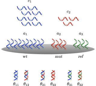
Figure 1: A minimal experimental setup for the study of target depletion. The sample solution (top) contains two targets, a wild-type (blue) and a mutant sequence (red), with concentrations $c_{1}$ and $c_{2}$, respectively. We assume the former to be in abundance, and the latter to be present in small traces, i.e. $c_{1}\gg c_{2}$. The two targets come into contact with three probes spotted on a surface (middle), with concentrations $a_{1}$, $a_{2}$ and $a_{3}$. The first two probes (blue and red) are the perfect complements of the two targets, while the third probe (green) is used as a reference for the detection of the mutant target. In order to achieve target depletion, we propose the use of a large concentration, $a_{1}$, of wild-type probes. Finally, at the bottom all possible duplexes are shown, together with the notation we employ.

More quantitively, the signal measured from each probe is the sum of the contributions from the wild type and the mutant, i.e. $\theta_{i}=\theta_{i1}+\theta_{i2}$. Probes mut and ref both have a single mismatch with respect to the wild-type target. By design we assume that their hybridization affinity to the wild type is similar, hence $\theta_{21}\approx\theta_{31}$, which can be achieved with a proper choice of the reference probe. In case a mutant target is present in solution ($c_{2}>0$), one has $\theta_{22}\gg\theta_{32}$, due to its much higher affinity for the second probe (perfect complement) than the third probe (two mismatches). Following Ref. 21, we define the detection signal as

$$S\equiv\log\frac{\theta_{2}}{\theta_{3}}=\log\frac{\theta_{21}+\theta_{22}}{\theta_{31}+\theta_{32}}\approx\log\left(1+\frac{\theta_{22}}{\theta_{21}}\right),$$ (10)

which will be zero when $c_{2}=0$ ($\theta_{22}=0$) and positive otherwise. Clearly, for diagnostic purposes we wish to have a large value of $S$ for small ratios $c_{2}/c_{1}$. Note that cross-hybridization can cause $\theta_{21}$ to be much larger than $\theta_{22}$, especially when $c_{1}\gg c_{2}$, hence obscuring the detection of the mutant target. In order to address this issue, we propose the use of a large concentration $a_{1}$ of wt, which will deplete the corresponding target, hence leading to a cleaner signal from mut. Though perhaps evident, this approach will also deplete the mutant target, and a profound quantitative analysis is needed to investigate this issue. In what follows, we will quantify this effect by considering both the equilibrium and kinetics of the hybridization process.

3.1 Equilibrium properties

We will first focus on the equilibrium aspects of target depletion. For a system with three probes, the hybridized probe fraction at equilibrium is given by [see Eq. (9)]

$$\widetilde{\theta}_{2j}=\frac{c_{j}K_{2j}}{1+a_{1}K_{1j}+a_{2}K_{2j}+a_{3}K_{3j}}.$$ (11)

The detection signal is then given by

$$S=\log\left(1+\frac{\widetilde{\theta}_{22}}{\widetilde{\theta}_{21}}\right)\approx\log\left(1+\frac{c_{2}}{c_{1}}\,\frac{K_{\text{PM}}}{K_{\text{1MM}}}\,\frac{1+a_{1}K_{\text{PM}}+a_{2}K_{\text{1MM}}+a_{3}K_{\text{1MM}}}{1+a_{1}K_{\text{1MM}}+a_{2}K_{\text{PM}}+a_{3}K_{\text{2MM}}}\right).$$ (12)

For simplicity, we have assumed that $K_{11}=K_{22}\equiv K_{\text{PM}}$, $K_{12}=K_{21}=K_{31}\equiv K_{\text{1MM}}$ and $K_{32}\equiv K_{\text{2MM}}$, associated with the perfect-match, single-mismatch and two-mismatch hybridizations, respectively. It is important to stress that the above relations are introduced for convenience and do not affect the main conclusions of this work. In absence of depletion ($a_{i}=0$), the detection signal becomes

$$S_{0}=\log\left(1+\frac{c_{2}}{c_{1}}\frac{K_{\text{PM}}}{K_{\text{1MM}}}\right)=\log\left(1+\frac{c_{2}}{c_{1}}e^{\Delta\Delta G_{\text{1MM}}/RT}\right),$$ (13)

where we have used the thermodynamic relation $K=e^{-\Delta G/RT}$, with $\Delta G$ the hybridization free energy, $R$ the gas constant and $T$ the temperature (note that by convention $\Delta G<0$). We have also introduced $\Delta\Delta G_{\text{1MM}}\equiv\Delta G_{\text{1MM}}-\Delta G_{\text{PM}}$, the free-energy difference between the perfect-match and one-mismatch hybridizations which depends on the mismatch identity and on flanking nucleotides, according to the nearest-neighbor model of DNA hybridization ^{22, 10, 11}. Equation (13) has been experimentally verified in the past (see e.g. Fig. 3 of Ref. 21), and shows that there are two factors controlling the detection limit of the device. One is the relative abundance, i.e. it is easier to detect mutants at high relative concentrations ($c_{2}/c_{1}$). The other factor is the relative affinity $\Delta\Delta G_{\text{1MM}}>0$, i.e. a large free energy penalty for mismatched hybridization leads to suppression of cross hybridization, and hence facilitates the detection of the mutant. Since typical values of $\Delta\Delta G_{\text{1MM}}$ lie in the range $1-4$ kcal/mol ¹⁰, and using the fact that the signal is detectable only when $S\geq S_{\text{min}}=0.5$ ²¹, it follows that the minimum relative concentration, $c_{2}/c_{1}$, that can be measured with this method lies in the range 0.17% to 15%, in agreement with previous reports ²¹. In this calculation we used $T=65^{\circ}$C as a typical system temperature ^{10, 23, 21}.

Next, we consider the other limit of strong depletion. We will assume the target depletion to occur only due to the wild-type probe, which can be tuned by choosing a large-enough probe concentration so that the condition $a_{1}K_{\text{1MM}}\gg a_{2}K_{\text{PM}}$ is met. Moreover, by fully exploiting the effect of target depletion, so that $a_{1}K_{\text{1MM}}\gg 1$, we obtain the following elegant expression

$$S\approx\log\left[1+\frac{c_{2}}{c_{1}}\left(\frac{K_{\text{PM}}}{K_{\text{1MM}}}\right)^{2}\right]=\log\left(1+\frac{c_{2}}{c_{1}}e^{2\Delta\Delta G_{\text{1MM}}/RT}\right).$$ (14)

By comparing Eqs. (13) and (14), we see that depleting the abundant wild-type target indeed leads to higher $S$ (additional factor of two in the exponent). Performing the same analysis as above, we find that the minimum relative concentration, $c_{2}/c_{1}$, that is experimentally detectable is in the range 0.00044% to 3.3%. This corresponds to an enhancement of the detection sensitivity by one to three orders of magnitude, owing to target depletion.

In order to experimentally realize the aforementioned detection enhancement, two conditions need to be met, as mentioned above. First, the relative concentration $a_{1}$ of the wild-type probes has to be much larger than those of the mutant and reference probes, so that

$$\frac{a_{1}}{a_{n}}\gg\frac{K_{\text{PM}}}{K_{\text{1MM}}}=e^{\Delta\Delta G_{\text{1MM}}/RT},$$ (15)

with $n=2,3$. Using typical values for hybridization free energies of single base pair mismatches (see above) we estimate $4\lesssim\exp(\Delta\Delta G_{\text{1MM}}/RT)\lesssim 400$. Thus, the larger the free-energy penalty, $\Delta\Delta G_{\text{1MM}}$, of a mismatch is, the larger the ratio $a_{1}/a_{n}$ ($n=2,3$) needed. Moreover, the absolute value of $a_{1}$ needs to be large enough, so as to maximize the contribution of depletion. The precise condition is

$$a_{1}\gg\frac{1}{K_{\text{1MM}}}=e^{\Delta G_{\text{1MM}}/RT}.$$ (16)

The precise value of $\Delta G_{\text{1MM}}/RT$ depends strongly on the DNA sequence, and can be estimated based on the nearest-neighbor model of DNA ²².

As a practical evaluation of these predictions, we also performed a DNA microarray experiment. The microarray contained two drastically-different groups of sequences, allowing us to study DNA hybridization both in absence and presence of target depletion (see Appendix for details). The solution contained both a wild-type and a mutant target, with relative proportion equal to $c_{2}/c_{1}=5\%$. In absence of depletion, the observed detection signal, as defined in Eq. (10), was found to be $S_{0}=0.9\pm 0.1$. On the other hand, target depletion was found to yield the value $S=4.5\pm 0.2$, corresponding to a five-fold enhancement of the detection signal (See details in Appendix). Interestingly, by taking $\Delta\Delta G_{\text{1MM}}=2.4$ kcal/mol, which is a reasonable value for the cost of a mismatch ¹⁰, Eqs. (13) and (14) yield $S_{0}\approx 1.0$ and $S\approx 4.2$, respectively. These values are remarkably close to the experimental ones, given the presence of a single free parameter.

Performing again the same analysis as above this leads to an estimated detection limit of the relative concentration $c_{2}/c_{1}$ of 1.8% for the non-depletion case and 0.052% for the depletion case. Hence the sensitivity is increased by a factor of 35 through target depletion.

3.2 Hybridization Kinetics

To investigate the kinetics of the system, we have numerically solved the coupled ODE (7). The wild-type concentration was fixed at the experimentally-realistic value of $c_{1}=50$ pM, while to obtain strong depletion we have set $a_{1}=800$ pM and $a_{2}=a_{3}=4$ pM. We considered on-rates identical for all sequences, which is supported to a good extent by experimental observations ²⁴. The value was set to $k_{+}=10^{6}$ $\text{s}^{-1}\text{M}^{-1}$. The off-rates were then fixed by the equilibrium condition $K\equiv k_{+}/k_{-}=e^{-\Delta G/RT}$. For the perfect-match, one- and two-mismatch hybridizations we used $\Delta G_{\text{PM}}=-16$ kcal/mol, $\Delta G_{\text{1MM}}=-13.5$ kcal/mol and $\Delta G_{\text{2MM}}=-11$ kcal/mol, respectively, based on nearest-neighbors data for a 15-mer at $T=65^{\circ}$C ²².

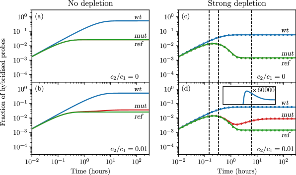
Figure 2: Hybridization evolution of a wild-type and a mutant target with an array of three probes, a wild-type (blue line), a mutant (red line) and a reference one (green line), for two values of the relative target concentration $r\equiv c_{2}/c_{1}$. Panels (a) and (b) correspond to the case where no depletion of the wild-type target takes place, whereas (c) and (d) to the strong depletion case, where the wild-type probe is in excess concentration. In the latter case, besides the numerical solution of Eqs. (7) (solid lines), we also plot the analytical solution (17) (points). The dashed vertical lines correspond to the three characteristic times, $t_{1}$, $t_{2}$ and $t_{3}$, discussed in the main text. The inset in (d) shows a magnification of the wt signal, revealing a very small overshoot.

Figure 2 shows the hybridization kinetics for $\theta_{i}$ in the case of no-depletion (a and b) and of strong depletion (c and d). The dots are the analytical solution, while the solid lines are obtained from the numerical integration of Eq. (7). In (a) and (c) the solution contains wild-type target at concentration $c_{1}=50$ pM and no mutant ($c_{2}=0$). The signals measured from mut and ref perfectly overlap, since we have assumed equal hybridization free energy $\Delta G_{\text{1MM}}$ for the two sequences. In (b) and (d) the solution additionally contains $c_{2}=0.5$ pM mutant (corresponding to a ratio $c_{2}/c_{1}=0.01$, i.e. $1\%$ of the wild-type concentration). Figure 2 indicates that the presence of the mutant is more easily detectable in the case of strong depletion as the gap between mut and ref is much more pronounced. The kinetics is also remarkably different: in absence of depletion the signal increases monotonically in time, whereas in the strong depletion case we observe a nonmonotonic behavior and even a dip in the signal from mut.

The long time behavior shown in Fig. 2 corresponds to the equilibrium solution given by Eq. (9). In order to understand the observed rich kinetics, one can use a simplified solvable case in which we assume that the depletion occurs due to the wt probe alone, i.e. $a_{2},a_{3}\approx 0$ and $a_{1}\equiv a\neq 0$. Under this approximation, the solution $\theta_{i}=\theta_{i1}+\theta_{i2}$ is found to be [see Eq. (31) of Appendix]

$$\theta_{1} =\frac{c_{1}K_{\text{PM}}}{1+aK_{\text{PM}}}\left[1-e^{-(ak_{+}+k_{\text{PM}})t}\right]+\frac{c_{2}K_{\text{1MM}}}{1+aK_{\text{1MM}}}\left[1-e^{-(ak_{+}+k_{\text{1MM}})t}\right],$$ (17)

$$\theta_{2} =\frac{c_{1}K_{\text{1MM}}}{1+aK_{\text{PM}}}\left\{1-e^{-k_{\text{1MM}}t}+\frac{K_{\text{PM}}}{K_{\text{1MM}}}\frac{ak_{+}}{ak_{+}+k_{\text{PM}}-k_{\text{1MM}}}\left[e^{-k_{\text{1MM}}t}-e^{-(ak_{+}+k_{\text{PM}})t}\right]\right\}$$

$$+\frac{c_{2}K_{\text{PM}}}{1+aK_{\text{1MM}}}\left\{1-e^{-k_{\text{PM}}t}+\frac{K_{\text{1MM}}}{K_{\text{PM}}}\frac{ak_{+}}{ak_{+}+k_{\text{1MM}}-k_{\text{PM}}}\left[e^{-k_{\text{PM}}t}-e^{-(ak_{+}+k_{\text{1MM}})t}\right]\right\},$$

$$\theta_{3} =\frac{c_{1}K_{\text{1MM}}}{1+aK_{\text{PM}}}\left\{1-e^{-k_{\text{1MM}}t}+\frac{K_{\text{PM}}}{K_{\text{1MM}}}\frac{ak_{+}}{ak_{+}+k_{\text{PM}}-k_{\text{1MM}}}\left[e^{-k_{\text{1MM}}t}-e^{-(ak_{+}+k_{\text{PM}})t}\right]\right\}$$

$$+\frac{c_{2}K_{\text{2MM}}}{1+aK_{\text{1MM}}}\left\{1-e^{-k_{\text{2MM}}t}+\frac{K_{\text{1MM}}}{K_{\text{2MM}}}\frac{ak_{+}}{ak_{+}+k_{\text{1MM}}-k_{\text{2MM}}}\left[e^{-k_{\text{2MM}}t}-e^{-(ak_{+}+k_{\text{1MM}})t}\right]\right\},$$

where we used $k_{\text{PM}}$, $k_{\text{1MM}}$ and $k_{\text{2MM}}$ to denote the off-rates, while $K_{\text{PM}}=k_{+}/k_{\text{PM}}$, $K_{\text{1MM}}=k_{+}/k_{\text{1MM}}$ and $K_{\text{2MM}}=k_{+}/k_{\text{2MM}}$. Equations (17) are shown in Fig. 2 as dotted lines and are in excellent agreement with numerics. One can further simplify them using the assumption $aK_{\text{PM}}>aK_{\text{1MM}}\gg 1$, which corresponds to the limit of strong depletion. This condition is satisfied for the parameters used in Fig. 2. Under this assumption, Eqs. (17) reduce to

$$\theta_{1} \approx\frac{c_{1}+c_{2}}{a}\left(1-e^{-ak_{+}t}\right),$$ (18)

$$\theta_{2} \approx\frac{c_{1}K_{\text{1MM}}}{aK_{\text{PM}}}\left[1-e^{-k_{\text{1MM}}t}+\frac{K_{\text{PM}}}{K_{\text{1MM}}}\left(e^{-k_{\text{1MM}}t}-e^{-ak_{+}t}\right)\right]$$

$$+\frac{c_{2}K_{\text{PM}}}{aK_{\text{1MM}}}\left[1-e^{-k_{\text{PM}}t}+\frac{K_{\text{1MM}}}{K_{\text{PM}}}\left(e^{-k_{\text{PM}}t}-e^{-ak_{+}t}\right)\right],$$

$$\theta_{3} \approx\frac{c_{1}K_{\text{1MM}}}{aK_{\text{PM}}}\left[1-e^{-k_{\text{1MM}}t}+\frac{K_{\text{PM}}}{K_{\text{1MM}}}\left(e^{-k_{\text{1MM}}t}-e^{-ak_{+}t}\right)\right].$$

In the last expression we have neglected the contribution $\theta_{32}$ of the mutant target to the probe ref, as the corresponding hybridization involves two mismatches and $c_{2}\ll c_{1}$. We, thus, identify three characteristic times, $t_{1}\equiv 1/ak_{+}$, $t_{2}\equiv 1/k_{\text{1MM}}$ and $t_{3}\equiv 1/k_{\text{PM}}$, which are ordered as $t_{1}<t_{2}<t_{3}$ and are shown as dashed vertical lines in panels (c) and (d) of Fig. 1. We note that, while $\theta_{1}$ is clearly a monotonic function of time, there are several time-dependent factors with opposite signs in $\theta_{2}$ and $\theta_{3}$, giving rise to nonmonotonic time evolution.

To analyze this time dependence in more detail, we first consider the regime in which $t\lesssim t_{1}$. In this time interval we approximate $\exp(-ak_{+}t)\approx 1-ak_{+}t$ and $\exp(-k_{\text{1MM}}t)\approx\exp(-k_{\text{PM}}t)\approx 1$, so as to get

$$\theta_{1}\approx\theta_{2}\approx\theta_{3}\approx\left(c_{1}+c_{2}\right)k_{+}t,$$ (19)

which indicates that at short time scales the kinetics is characterized by an identical binding rate to wt, mut and ref. This is because we have assumed equal attachment rate $k_{+}$ for all probes and targets, which is a reasonable approximation. This, however, does not influence the main features of the kinetics at the subsequent time scales. In the next interval $t_{1}\ll t\lesssim t_{2}$, we approximate $\exp(-ak_{+}t)\approx 0$ and $\exp(-k_{\text{PM}}t)\approx 1$. In this case the wt probe signal reaches a stationary value $\theta_{1}\approx(c_{1}+c_{2})/a$, which can also be obtained from the equilibrium solution (9), while

$$\theta_{2} \approx\frac{c_{1}}{a}\left[\frac{K_{\text{1MM}}}{K_{\text{PM}}}+\left(1-\frac{K_{\text{1MM}}}{K_{\text{PM}}}\right)e^{-k_{\text{1MM}}t}\right]+\frac{c_{2}}{a},$$ (20)

$$\theta_{3} \approx\frac{c_{1}}{a}\left[\frac{K_{\text{1MM}}}{K_{\text{PM}}}+\left(1-\frac{K_{\text{1MM}}}{K_{\text{PM}}}\right)e^{-k_{\text{1MM}}t}\right],$$

which, as $K_{\text{PM}}>K_{\text{1MM}}$, are decreasing functions of time. In this regime the wild-type target starts dissociating at the same rate $k_{\text{1MM}}$ from mut and ref probes. This leads to a very weak increase in the hybridization of the wt probe, which is not detectable in the scale of Fig. 2 (see inset of panel d), and also not present in the approximated solution (18). This weak increase is, however, present in the full solution (17). Finally, at even longer times, i.e. for $t_{2}\ll t\sim t_{3}$, one has $\exp(-ak_{+}t)\approx\exp(-k_{\text{1MM}}t)\approx 0$. The ref probe reaches a steady state $\theta_{3}\approx c_{1}K_{\text{1MM}}/(aK_{\text{PM}})$, while the mut probe increases monotonically as

$$\theta_{2} \approx\frac{c_{1}}{a}\frac{K_{\text{1MM}}}{K_{\text{PM}}}+\frac{c_{2}}{a}\left[\frac{K_{\text{PM}}}{K_{\text{1MM}}}-\left(\frac{K_{\text{PM}}}{K_{\text{1MM}}}-1\right)e^{-k_{\text{PM}}t}\right].$$ (21)

This increase takes place only if $c_{2}>0$, while in absence of mutant target ($c_{2}=0$) this third timescale is absent, and mut reaches a steady state value from above as ref. In this last regime the wild-type target has completely equilibrated, and the mutant target gets redistributed from the wt probe to the mut probe. This gives rise to a monotonic increase in the hybridization of the latter, until the complete equilibration of the system. The turnover time at which $\theta_{2}$ is minimal can be calculated from Eqs. (18) and is given by

$$t_{\text{min}}=\frac{\log(c_{1}/c_{2})}{k_{\text{1MM}}-k_{\text{PM}}}.$$ (22)

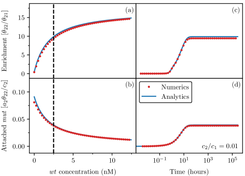
Figure 3: Upper panels: Mutant/wild-type target ratio, $\theta_{22}/\theta_{21}$, attached to the mut probe. Higher values of the ratio enable the further enrichment of the sample, by increasing the relative population of the mutant with respect to the wild-type target. Lower panels: Fraction, $a_{2}\theta_{22}/c_{2}$, of the mutant target that has hybridized with the mut probe. For application purposes, the concentration, $a_{2}\theta_{22}$, of the captured mutant target should be comparable to the initial one, $c_{2}$, in solution. These quantities are plotted both (a,b) as a function of the wt probe concentration at equilibrium and (c-d) as a function of time at a fixed wt probe concentration ($a_{1}=2.5$ nM, corresponding to the dashed vertical lines). The small deviation between analytics and numerics arises from the approximation $a_{2},a_{3}\approx 0$ included in the former.

Next, we show how target depletion can be used for sample enrichment, i.e. increasing the relative amount of mutant DNA over wild-type DNA. From an application point of view, this is an important issue, and can lead to an increased performance for mutant detection by other techniques, such as sequencing ^{25, 26}. Hereto, we focus on the hybridized material on the mut probe (probe number 2) and study two important quantities (see Fig. 3): the ratio of mutant over wild-type target attached to mut (a,c) and the absolute amount of mutant target (b,d). The former quantity determines whether we can achieve enrichment, the latter is needed as a measure of capture efficiency. In Fig. 3 (a) and (b) these quantities are plotted as functions of depletion (i.e. wt probe concentration, $a_{1}$), for a sample with starting target mutant ratio of $c_{2}/c_{1}=0.01$. These plots quantitatively show how depletion leads to a trade-off between yield and sample enrichment. As an example, indicated with the dashed vertical line, is a regime where a yield of about 4% gives a mutant enrichment of a factor $(\theta_{22}/\theta_{21})/(c_{2}/c_{1})\approx 940$. Finally, the kinetics shown in Fig. 3 (c) and (d) indicates that the quantities evolve monotonically in time, hence equilibrium conditions can be used to achieve the best results.

4 Conclusion

In this paper we have analyzed the equilibrium and kinetics of hybridization in DNA biosensors under the effect of strong target depletion. This is a condition which has been considered only in limited prior studies ^{13, 14, 15} since the typical assumption behind hybridization models in DNA biosensors, as the Langmuir adsorption model, is that the target sequences in solution are in excess. Target concentration is then considered to be constant throughout the duration of the experiment. To fulfill this condition one needs a sufficient amount of hybridizing material to start with. Although target depletion is typically avoided, our analysis shows that one can turn it, in some applications, into an advantageous condition, leading to an increase of the performance of the biosensor.

We focused on the problem of detection of small amount of mutant sequence (with concentration $c_{2}$) diluted in a highly-abundant wild type (with concentration $c_{1}$), and specifically addressed the case of a single nucleotide difference between the two. An example where this is an important diagnostic problem is in liquid biopsy, where one examines a mixture of “healthy” molecules in majority, with a small subpopulation of molecules carrying a specific pathogenic property.

The minimal design employed in this study involves three probe sequences, which we referred to as wild-type (wt), mutant (mut) and reference (ref) probe. The presence of the mutant in solution is inferred by the ratio of hybridization signals measured from ref and mut. We have presented a quantitative analysis of the hybridization kinetics and shown that in presence of wild-type depletion one can decrease the detection limit up to three orders of magnitudes in the ratio $c_{2}/c_{1}$ [as revealed by a comparison between Eqs. (13) and (14)]. Note that the only sequence-dependent parameter controlling the detection limit is the free energy penalty associated to a single mismatch. With the same design we showed that, next to detection, also target enrichment can be enhanced.

Finally, our analysis of the kinetics revealed a rich behavior, with interplay between the initial strong binding of target, followed by unbinding and redistribution of the sequences between the different probes. This resulted in three different time scales and a mut signal that exhibits a nonmonotonic behavior: an increase followed by a decrease and then by a final increase towards equilibrium. We expect that this distinct feature, which we have found to take place only when $c_{2}>0$, should be observable in experiments which have access to the kinetics of hybridization. ^{27, 28}

We acknowledge financial support from the Research Funds Flanders (FWO Vlaanderen) Grant No. VITO-FWO 11.59.71.7N.

Appendix A Appendix

A.1 DNA microarray experiment

To confirm the detection enhancement predicted by Eqs. (13) and (14), we performed a microarray experiment. We designed two sets of wild-type, mutant and reference probes, shown in Table 1. The first probe set was based on previously-published data ²¹, from which we selected the optimal double-mismatch ref probe for the wt and mut pair, i.e. one for which $|\theta_{21}-\theta_{31}|$ is minimised. (Note that the selected ref probe which best fulfilled this criteron actually contains two mismatches with respect to the wild-type target and three to the mutant target, in contrast to the one- and two-mismatch case described in the main text. The number of mismatches is not critical here, but rather the relative $\Delta\Delta G$ values.)

The second probe set was designed to maintain the sequences and positions of the variable triplets from the first set, as well as a similar overall $\Delta G_{\text{PM}}$, while the remainder of the sequence was kept distinct to avoid cross-hybridisation.

The six probes were laid out on the array, which contained 10 spots of the $wt_{0}$ probe and $1.5\times 10^{4}$ spots of the $wt_{\text{dep}}$ probe, corresponding to the no depletion and strong depletion regimes. The array was incubated with a mixture of $wt$ and $mut$ targets for each probe set (Table 2), with $c_{2}/c_{1}=0.05$. Targets for the two probe sets were labelled with different fluorophores, allowing them to be measured independently on the same array. The results are shown in Figure 4.

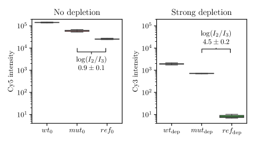
Figure 4: Microarray fluorescence intensity data showing the effect of depletion on the relative mutant hybridisation signal.

	Probe	Sequence (5’ - 3’)	Array replicates
Depletion	$wt_{\text{dep}}$	GTTG GAG CT GGT GGC GTA GGCAA	15158
	$mut_{\text{dep}}$	GTTG GAG CT GCT11GCT22GCT33 GGC GTA GGCAA	10
	$ref_{\text{dep}}$	GTTG GGG11GGG22GGG33 CT GGT GGC GAA11GAA22GAA33 GGCAA	10
No depletion	$wt_{0}$	CGCC GAG TC GGT CAT GTA CTGGC	10
	$mut_{0}$	CGCC GAG TC GCT11GCT22GCT33 CAT GTA CTGGC	10
	$ref_{0}$	CGCC GGG11GGG22GGG33 TC GGT CAT GAA11GAA22GAA33 CTGGC	10

Table 1: Microarray probe sequences used in the experiment.

	Target	Sequence (5’ - 3’)	Concentration
Depletion	$T_{wt,{\text{dep}}}$	TTGCCTACGCC ACC AGCTCCAAC+Cy3	95 pM
	$T_{mut,{\text{dep}}}$	TTGCCTACGCC AGC11AGC22AGC33 AGCTCCAAC+Cy3	5 pM
No depletion	$T_{wt,{0}}$	GCCAGTACATG ACC GACTCGGCG+Cy5	95 pM
	$T_{mut,{0}}$	GCCAGTACATG AGC11AGC22AGC33 GACTCGGCG+Cy5	5 pM

Table 2: Target sequences used in the microarray experiment.

A.1.1 Materials and methods

A custom 8x15K Agilent microarray slide was used (Agilent Technologies, US). Microarray probes all included a $(\text{dA})_{30}$ linker sequence on the 3’ end. Target oligonucleotides (IDT, Germany) included a $(\text{dA})_{20}$ linker and a Cy3 or Cy5 fluorescent dye on the 3’ end. Target oligonucleotides were mixed to final concentrations shown in Table 2 in $1\times$ Agilent GEx hybridisation buffer HI-RPM with $1\times$ Agilent GE blocking agent. The slide was incubated with 40 $\mathrm{\SIUnitSymbolMicro L}$ of this target mixture in an Agilent hybridisation oven for 17 hours at 65$\mathrm{\SIUnitSymbolCelsius}$ with rotor setting 10, followed by washing according to manufacturer instructions. An Agilent G2565BA scanner was used to image the microarray, with a 5-$\mathrm{\SIUnitSymbolMicro m}$ resolution and 100% gain. Image analysis was carried out using the Agilent Feature Extraction software, version 10.7. The signal was background-corrected by subtraction of the global minimum signal.

A.2 Equilibrium isotherm and the Sherman-Morrison formula

In order to compute the fraction of hybridized probes at equilibrium, it is convenient to introduce a vector $\boldsymbol{\theta}$, defined as $\boldsymbol{\theta}\equiv\{\theta_{11},\theta_{21},\ldots,\theta_{n_{\text{p}}1},\theta_{12},\theta_{22},\ldots,\theta_{n_{\text{p}}2},\ldots\}$. With this definition, one can cast Eq. (8) in matrix form

$$\frac{\text{d}\boldsymbol{\theta}}{\text{d}t}=-\mathbf{M}\boldsymbol{\theta}+\mathbf{b},$$ (23)

where $\mathbf{M}$ is a block diagonal matrix. The j-th block, $\mathbf{M}^{j}$, corresponds to the contribution from a single target $j$ and mixes the elements of the subvector ${\boldsymbol{\theta}}^{j}\equiv\{\theta_{1j},\theta_{2j},\ldots,\theta_{n_{\text{p}}j}\}$. Its entries are

$$M^{j}_{nm}=k^{+}_{nj}a_{m}+k^{-}_{nj}\delta_{nm},$$ (24)

where $\delta_{nm}$ indicates the Kronecker $\delta$ function. In the $j$-th block, the constant vector is given by $\mathbf{b}^{j}_{n}=k^{+}_{nj}c_{j}$. The equilibrium value $\widetilde{\boldsymbol{\theta}}$ is obtained by inverting the matrix $\mathbf{M}$ as

$$\widetilde{\boldsymbol{\theta}}=\mathbf{M}^{-1}\mathbf{b},$$ (25)

which can be performed independently for each block. In order to calculate $\mathbf{M}^{-1}$, we notice that the j-th block of $\mathbf{M}$ is the sum of a diagonal matrix and the outer product of two vectors, i.e. $\mathbf{M}^{j}=\mathbf{D}+\mathbf{u}\mathbf{v}^{\text{T}}$, with $\mathbf{D}$ diagonal and $\mathbf{u}\mathbf{v}^{\text{T}}\equiv\mathbf{u}\otimes\mathbf{v}$. This allows us to use the Sherman-Morrison formula, which reads

$$\left(\mathbf{D}+\mathbf{u}\mathbf{v}^{\text{T}}\right)^{-1}=\mathbf{D}^{-1}-\frac{\mathbf{D}^{-1}\mathbf{u}\mathbf{v}^{\text{T}}\mathbf{D}^{-1}}{1+\mathbf{v}^{\text{T}}\mathbf{D}^{-1}\mathbf{u}},$$ (26)

(note that, while $\mathbf{u}\mathbf{v}^{\text{T}}$ is an $n_{\text{p}}\times n_{\text{p}}$ matrix, $\mathbf{v}^{\text{T}}\mathbf{D}^{-1}\mathbf{u}$ is a scalar). In the present case $\mathbf{D}=\text{diag}\{k^{-}_{1j},k^{-}_{2j},k^{-}_{3j},\ldots\}$, while the two vectors are $\mathbf{u}=\{k^{+}_{1j},k^{+}_{2j},k^{+}_{3j},\ldots\}$ and $\mathbf{v}=\{a_{1},a_{2},a_{3},\ldots\}$. Using the above definitions, together with $\mathbf{b}^{j}=c_{j}\mathbf{u}$, we find the following equilibrium solution of the $j$-th block:

$$\widetilde{\boldsymbol{\theta}^{j}}=\left(\mathbf{M}^{j}\right)^{-1}\mathbf{b}^{j}=c_{j}\ \left(\mathbf{D}+\mathbf{u}\mathbf{v}^{\text{T}}\right)^{-1}\mathbf{u}=\frac{c_{j}\mathbf{D}^{-1}\mathbf{u}}{1+\mathbf{v}^{\text{T}}\mathbf{D}^{-1}\mathbf{u}}.$$ (27)

A simple calculation gives

$$\mathbf{v}^{T}\mathbf{D}^{-1}\mathbf{u}=\sum_{n=1}^{n_{\text{p}}}a_{n}K_{nj}\qquad\text{and}\qquad\mathbf{D}^{-1}\mathbf{u}=\{K_{1j},K_{2j},K_{3j},\ldots\},$$ (28)

where $K_{ij}\equiv k^{+}_{ij}/k^{-}_{ij}$ is the equilibrium constant. Combining Eqs. (27) and (28), and recalling that $\widetilde{\boldsymbol{\theta}^{j}}_{i}=\widetilde{\theta}_{ij}$, we finally obtain Eq. (9).

A.3 Hybridization kinetics under depletion by a single sequence

Equation (23) can be analytically solved when depletion occurs due to a single probe. In this case we can write

$$\frac{\text{d}\theta_{ij}}{\text{d}t}=k_{ij}^{+}\left(c_{j}-\sum_{n=1}^{n_{\text{p}}}a_{n}\theta_{nj}\right)-k_{ij}^{-}\theta_{ij}\approx k_{ij}^{+}\left(c_{j}-a_{1}\theta_{1j}\right)-k_{ij}^{-}\theta_{ij},$$ (29)

where we have assumed that $a_{n}\ll c_{j}$ for $n>1$. This condition can be experimentally realized through a proper design of the probes and choice of target concentrations. Under this assumption, one has a set of independent equations for $\theta_{1j}$ that can be easily solved

$$\theta_{1j}=\frac{c_{j}K_{1j}}{1+a_{1}K_{1j}}\left[1-e^{-(a_{1}k_{1j}^{+}+k_{1j}^{-})t}\right],$$ (30)

which is monotonically growing in time and approaches the stationary value $\widetilde{\theta}_{1j}=c_{j}K_{1j}/(1+a_{1}K_{1j})$. One can plug Eq. (30) in (29) to solve for the remaining $\theta_{ij}$ with $i>1$. The result is

$$\theta_{ij}=\frac{c_{j}K_{ij}}{1+a_{1}K_{1j}}\left[1-e^{-t/\tau_{ij}}+\frac{k_{ij}^{-}}{k_{1j}^{-}}\frac{a_{1}k_{1j}^{+}}{a_{1}k_{1j}^{+}+k_{1j}^{-}-k_{ij}^{-}}\left(e^{-t/\tau_{ij}}-e^{-t/\tau_{1j}}\right)\right],$$ (31)

where $\tau_{ij}\equiv(a_{1}k_{ij}^{+}\delta_{i1}+k_{ij}^{-})^{-1}$ is a characteristic time. Note that by setting $i=1$ in Eq. (31), one recovers Eq. (30), as the third term within the square brackets vanishes. Thus, Eq. (31) can be used as a general solution of the problem for all $i$ and $j$.

References

- Naef et al. 2002 Naef, F.; Lim, D. A.; Patil, N.; Magnasco, M. DNA hybridization to mismatched templates: a chip study. Phys. Rev. E 2002, 65, 040902
- Vainrub and Pettitt 2002 Vainrub, A.; Pettitt, B. M. Coulomb blockage of hybridization in two-dimensional DNA arrays. Phys. Rev. E 2002, 66, 041905
- Held et al. 2003 Held, G.; Grinstein, G.; Tu, Y. Modeling of DNA microarray data by using physical properties of hybridization. Proceedings of the National Academy of Sciences 2003, 100, 7575–7580
- Zhang et al. 2003 Zhang, L.; Miles, M. F.; Aldape, K. D. A model of molecular interactions on short oligonucleotide microarrays. Nature biotechnology 2003, 21, 818
- Halperin et al. 2004 Halperin, A.; Buhot, A.; Zhulina, E. Sensitivity, specificity, and the hybridization isotherms of DNA chips. Biophys. J. 2004, 86, 718–730
- Binder and Preibisch 2005 Binder, H.; Preibisch, S. Specific and nonspecific hybridization of oligonucleotide probes on microarrays. Biophys. J. 2005, 89, 337–352
- Burden et al. 2006 Burden, C. J.; Pittelkow, Y.; Wilson, S. R. Adsorption models of hybridization and post-hybridization behaviour on oligonucleotide microarrays. J. Phys.: Cond. Matter 2006, 18, 5545
- Carlon and Heim 2006 Carlon, E.; Heim, T. Thermodynamics of RNA/DNA hybridization in high-density oligonucleotide microarrays. Physica A 2006, 362, 433
- Naiser et al. 2009 Naiser, T.; Kayser, J.; Mai, T.; Michel, W.; Ott, A. Stability of a surface-bound oligonucleotide duplex inferred from molecular dynamics: a study of single nucleotide defects using DNA microarrays. Phys. Rev. Lett. 2009, 102, 218301
- Hooyberghs et al. 2009 Hooyberghs, J.; Van Hummelen, P.; Carlon, E. The effects of mismatches on hybridization in DNA microarrays: determination of nearest neighbor parameters. Nucleic Acids Res. 2009, 37, e53–e53
- Hadiwikarta et al. 2012 Hadiwikarta, W. W.; Walter, J.-C.; Hooyberghs, J.; Carlon, E. Probing hybridization parameters from microarray experiments: nearest-neighbor model and beyond. Nucleic Acids Res. 2012, 40, e138
- Harrison et al. 2013 Harrison, A. et al. Physico-chemical foundations underpinning microarray and next-generation sequencing experiments. Nucl. Acids Res. 2013, 41, 2779–2796
- Michel et al. 2007 Michel, W.; Mai, T.; Naiser, T.; Ott, A. Optical study of DNA surface hybridization reveals DNA surface density as a key parameter for microarray hybridization kinetics. Biophys. J. 2007, 92, 999–1004
- Ono et al. 2008 Ono, N.; Suzuki, S.; Furusawa, C.; Agata, T.; Kashiwagi, A.; Shimizu, H.; Yomo, T. An improved physico-chemical model of hybridization on high-density oligonucleotide microarrays. Bioinformatics 2008, 24, 1278–1285
- Burden and Binder 2009 Burden, C. J.; Binder, H. Physico-chemical modelling of target depletion during hybridization on oligonulceotide microarrays. Phys. Biol. 2009, 7, 016004
- Ang and Yung 2012 Ang, Y. S.; Yung, L.-Y. L. Rapid and label-free single-nucleotide discrimination via an integrative nanoparticle–nanopore approach. ACS Nano 2012, 6, 8815–8823
- Mohammadi-Kambs et al. 2017 Mohammadi-Kambs, M.; Hölz, K.; Somoza, M. M.; Ott, A. Hamming Distance as a Concept in DNA Molecular Recognition. ACS Omega 2017, 2, 1302–1308
- Su et al. 2017 Su, X.; Li, L.; Wang, S.; Hao, D.; Wang, L.; Yu, C. Single-molecule counting of point mutations by transient DNA binding. Sci. Rep. 2017, 7, 43824
- Rapisarda et al. 2017 Rapisarda, A.; Giamblanco, N.; Marletta, G. Kinetic discrimination of DNA single-base mutations by localized surface plasmon resonance. J. Colloid Interface Sci. 2017, 487, 141–148
- Zhang et al. 2018 Zhang, J. X.; Fang, J. Z.; Duan, W.; Wu, L. R.; Zhang, A. W.; Dalchau, N.; Yordanov, B.; Petersen, R.; Phillips, A.; Zhang, D. Y. Predicting DNA hybridization kinetics from sequence. Nat. Chem. 2018, 10, 91
- Willems and et al. 2017 Willems, H.; et al., Thermodynamic framework to assess low abundance DNA mutation detection by hybridization. PloS One 2017, 12, e0177384
- SantaLucia Jr and Hicks 2004 SantaLucia Jr, J.; Hicks, D. The thermodynamics of DNA structural motifs. Annu. Rev. Biophys. Biomol. Struct. 2004, 33, 415–440
- Hooyberghs et al. 2010 Hooyberghs, J.; Baiesi, M.; Ferrantini, A.; Carlon, E. Breakdown of thermodynamic equilibrium for DNA hybridization in microarrays. Phys. Rev. E 2010, 81, 012901
- Glazer et al. 2006 Glazer, M.; Fidanza, J. A.; McGall, G. H.; Trulson, M. O.; Forman, J. E.; Suseno, A.; Frank, C. W. Kinetics of oligonucleotide hybridization to photolithographically patterned DNA arrays. Anal. Biochem. 2006, 358, 225–238
- Samorodnitsky et al. 2015 Samorodnitsky, E.; Jewell, B. M.; Hagopian, R.; Miya, J.; Wing, M. R.; Lyon, E.; Damodaran, S.; Bhatt, D.; Reeser, J. W.; Datta, J.; Roychowdhury, S. Evaluation of hybridization capture versus amplicon-based methods for whole-exome sequencing. Hum. Mutat. 2015, 36, 903–914
- Khodakov et al. 2016 Khodakov, D.; Wang, C.; Zhang, D. Y. Diagnostics based on nucleic acid sequence variant profiling: PCR, hybridization, and NGS approaches. Adv. Drug Deliv. Rev. 2016, 105, 3–19
- Vermeeren et al. 2007 Vermeeren, V.; Bijnens, N.; Wenmackers, S.; Daenen, M.; Haenen, K.; Williams, O. A.; Ameloot, M.; vandeVen, M.; Wagner, P.; Michiels, L. Towards a real-time, label-free, diamond-based DNA sensor. Langmuir 2007, 23, 13193–13202
- Van Grinsven et al. 2011 Van Grinsven, B. et al. Rapid assessment of the stability of DNA duplexes by impedimetric real-time monitoring of chemically induced denaturation. Lab Chip 2011, 11, 1656–1663
For Table of Contents only