Dimensional crossover in the aging dynamics of spin glasses in a film geometry

Abstract

Motivated by recent experiments of exceptional accuracy, we study numerically the spin-glass dynamics in a film geometry. We cover all the relevant time regimes, from picoseconds to equilibrium, at temperatures at and below the 3D critical point. The dimensional crossover from 3D to 2D dynamics, that starts when the correlation length becomes comparable to the film thickness, consists of four dynamical regimes. Our analysis, based on a Renormalization Group transformation, finds consistent the overall physical picture employed by Orbach et al. in the interpretation of their experiments.

I Introduction

Spin glass physics Mézard et al. (1987); Fisher and Hertz (1991) has interested, puzzled and motivated the scientific community in the last fifty years, and it is still full of open challenges. The models behind this approach are both of dramatic theoretical and computational interest and of widespread potential interest, since they describe very different systems and situations. Glassy physics and the outstanding problem of the explanation of the amorphous state can receive important clarifications from the ideas developed in this context. Besides, very diverse fields like neuroscience, optimization, active matter, protein folding or DNA and RNA physics are turning out to be connected to the field and, indeed, progress thanks to the same techniques Young (1998).

In the lab, spin-glass samples are permanently out of equilibrium when studied at temperatures below the critical one, $T_{\mathrm{c}}$, implying that the equilibrium theory is not always sufficient. A possible approach to overcome this difficulty is extracting from the non-equilibrium dynamics crucial information about the (so difficult to reach) equilibrium regime Cugliandolo and Kurchan (1993); Franz et al. (1999); Alvarez Baños et al. (2010); Baity-Jesi et al. (2017a). However, custom-built computers Baity-Jesi et al. (2014) and other simulation advances Manssen and Hartmann (2015); Fernández and Martín-Mayor (2015) have made it possible to study theoretically Belletti et al. (2008, 2009); Manssen et al. (2015); Baity-Jesi et al. (2017b, 2018); Fernández et al. (2019, 2018) the simplest experimental protocol. In this protocol, see e.g. Joh et al. (1999), a spin glass at some very high-temperature is fastly quenched to the working temperature $T<T_{\mathrm{c}}$ and the excruciatingly slow growth of the spin-glass correlation length $\xi$ is afterwards studied as a function of the time elapsed since the quench, $t$. Although simulations do not approach yet the experimental time and length scales ($t\sim 1$ hour and $\xi\sim 100\,a_{0}$, where $a_{0}$ is the average distance between magnetic moments), the range covered is already significant: from picoseconds to milliseconds Manssen and Hartmann (2015); Fernández and Martín-Mayor (2015) or even 0.1 seconds using dedicated computers Belletti et al. (2008); Baity-Jesi et al. (2018) (or conventional ones in the case of two-dimensional spin glasses Fernández et al. (2019, 2018)).

Yet, thanks to advances in sample preparation, a new and promising experimental protocol have appeared in the last five years. Indeed, single-crystal spin glass samples with a thin-film geometry (thickness of $4.5-20$ nm) have been investigated Guchhait and Orbach (2014, 2017); Zhai et al. (2017); Kenning et al. (2018). These experiments are interpreted in terms of a correlation length $\xi$ saturating at a constant value after reaching a characteristic length scale, namely the thickness of the film. The bounded growth of $\xi$ along the longitudinal direction of the film is a direct experimental confirmation Guchhait and Orbach (2014) for a lower critical dimension $2<D_{\text{l}}^{\text{c}}<3$, in agreement with the theoretical expectation $D_{\text{l}}^{\text{c}}\sim 2.5$ Bray et al. (1986); Franz et al. (1994); Maiorano and Parisi (2018). The film-geometry has allowed as well for extremely accurate measurements Zhai et al. (2017) of the aging rate

$$z(T,\xi)=\frac{\mathrm{d}\,\log t}{\mathrm{d}\,\log\xi}\,,$$ (1)

which gives access to the dominant free-energy barrier $\varDelta$, $t\sim\tau_{0}\,\text{exp}[\varDelta/(k_{\text{B}}T)]$  [$\tau_{0}=\hbar/(k_{\text{B}}T_{\mathrm{c}})$ is a time scale]. The increased accuracy has shown that, contrary to previous expectations Joh et al. (1999); Belletti et al. (2008, 2009); Baity-Jesi et al. (2017b), the aging rate depends on $\xi$ (see also Bert et al. (2004); Baity-Jesi et al. (2018)). Besides, the dependency of the barrier $\varDelta$ with the applied magnetic field has been clarified Guchhait and Orbach (2017). However, a theoretical study of these fascinating thin-film experiments is lacking.

Here, we investigate the spin glass dynamics in a film geometry through large-scale numerical simulations. We analyze the dimensional-crossover and we critically assess the hypothesis of a dynamical arrest that becomes complete as soon as transversal saturation of the correlation length happens. Somewhat surprisingly, we find a rich dynamic behavior with no less than four different regimes (3D growth at short times, a double crossover regime with a faster growth for intermediate times, and a final equilibration regime). We analyze our results by combining the phenomenological Renormalization Group Nightingale (1976) with recent analysis of the two-dimensional spin glass dynamics Fernández et al. (2019, 2018). On the light of our results, the interpretation of thin-film experiments Guchhait and Orbach (2014, 2017); Zhai et al. (2017); Kenning et al. (2018) seems essentially correct, albeit slightly oversimplified.

The remaining part of this work is organized as follows. In Sect. II we recall the spin glass physics in $2\text{D}$ and $3\text{D}$. In Sect. III we define the model and provide details about our simulation and our analysis protocol. Our main results are given in Sect. IV, where we discovered a dynamics characterized by four aging regimes and through the Renormalization Group approach we found a non-trivial temperature mapping between a film and a 2D system. Finally, we provide our conclusions in Sect. V. Further details are provided in the appendices.

II 2D and 3D spin glass dynamics

Before addressing the dimensional crossover, let us recall a few crucial facts about the very different dynamic behavior of spin glasses in spatial dimensions $D=2$ Fernández et al. (2019, 2018) and $D=3$ Baity-Jesi et al. (2018).

In 3D, a phase transition at $T\!=\!T_{\mathrm{c}}$ separates the high-temperature paramagnetic phase from the spin-glass phase Gunnarsson et al. (1991); Palassini and Caracciolo (1999); Ballesteros et al. (2000). The aging rate (1) is $\xi$-independent at exactly $T=T_{\mathrm{c}}$, which results into a power-law dynamics $\xi\sim t^{1/z(T_{\mathrm{c}})}$, with $z(T_{\mathrm{c}})=6.69(6)$. At $T<T_{\mathrm{c}}$, but only once $\xi$ grows large-enough Baity-Jesi et al. (2018), the aging-rate grows with $\xi$ (the dynamics slows-down, and a power-law description is no longer appropriate). A simplifying feature is that the renormalized aging-rage $z(T,\xi)T/T_{\mathrm{c}}$ is roughly $T$-independent: when $T<T_{\mathrm{c}}$, the dominant barrier $\varDelta(\xi)$ depends little (or not at all) on temperature.

In 2D, we are in the paramagnetic phase for any $T>0$. Hence, $\xi(t,T)$ eventually reaches its equilibrium limit $\xi_{\text{eq}}(T)$, which can be very large Fernández et al. (2016, 2019): for $T\to 0$, $\xi_{\text{eq}}(T)\propto 1/T^{\nu_{\text{2D}}}$, $\nu_{\text{2D}}=3.580(4)$ Khoshbakht and Weigel (2018). When $a_{0}\ll\xi(t,T)\ll\xi_{\text{eq}}(T)$ we have a power law $\xi\propto t^{1/z_{\text{2D}}}$, with $z_{\text{2D}}\approx 7.14\,$ irrespective of $T$ Fernández et al. (2019): 2D dynamics may be much faster than 3D dynamics (aging rates $z\sim 15$ are not uncommon in 3D at low $T$). For times scale $t\gg\tau^{\text{2D}}_{\text{eq}}(T)$ equilibrium is approached. A super-Arrhenius behavior is found for $\tau^{\text{2D}}_{\text{eq}}(T)\propto\text{exp}[\varDelta^{\text{2D}}(\xi_{\text{eq}})/T]$, where the barrier $\varDelta^{\text{2D}}(\xi_{\text{eq}})$ grows very mildly with $\xi_{\text{eq}}$ Fernández et al. (2019).

III Model and protocol

We consider the Edwards-Anderson model Edwards and Anderson (1975) in a cubic lattice with a film geometry. Our films have two long sides of length $L_{x}=L_{y}$, and thickness $L_{z}\ll L_{x}$ (in the experiments, $L_{z}$ ranges from 8 to 38 layers Zhai et al. (2017)). We impose periodic boundary conditions (PBC) along the two longitudinal directions $X$ and $Y$. We have simulated $L_{x}=256$ and $L_{z}=4$, 6, 8 and 16. We always keep $L_{x}\gg\xi$, in order to effectively take the $L_{x}\to\infty$ limit. On the other hand, we have considered both PBC and open boundary conditions (OBC) along the short transversal direction $Z$. For simplicity, we discuss here only PBC [see appendix C for the qualitatively similar OBC results].

At the initial time $t=0$ our fully disordered films are abruptly quenched down to the working temperature $T$, which we simulate with Metropolis dynamics ($t$ is measured in full-lattice sweeps, a sweep roughly corresponds to 1 picosecond Mydosh (1993)). Our $\sigma_{\bm{x}}=\pm 1$ spins interact with their lattice nearest-neighbors through a Hamiltonian $H_{\mathrm{EA}}=-\sum_{<\bm{x},\bm{y}>}J_{\bm{x}\bm{y}}\,\sigma_{\bm{x}}\,\sigma_{\bm{y}}$, where the quenched disordered couplings are $\{J_{\bm{x}\bm{y}}\}=\pm 1$ with $50\%$ probability. For each quenched realization of the coupling (a sample) we study $N_{\mathrm{R}}$ real replicas. $N_{\mathrm{R}}$ has been selected for optimal performances (see appendices A and B for further details).

The spatial autocorrelation function Belletti et al. (2009) is defined as $C_{4}\left(T,\bm{r},t\right)=\overline{\left\langle q^{(a,b)}\left(\bm{x},t\right)q^{(a,b)}\left(\bm{x}+\bm{r},t\right)\right\rangle_{T}}\,,$ $q^{(a,b)}\left(\bm{x},t\right)\equiv\sigma^{(a)}\left(\bm{x},t\right)\sigma^{(b)}\left(\bm{x},t\right)\,,$ where the indices $(a,b)$ label the different real replicas, $\overline{(\cdots)}$ denotes the average over the disorder and $\langle\cdots\rangle_{T}$ stands for the average over the thermal noise at temperature $T$.

For the longitudinal lattice displacements $\bm{r}=(r,0,0)$ or $(0,r,0)$, one expects Parisi (1988); Fernández et al. (2018)

$$C_{4}\left(T,\bm{r},t\right)\sim\frac{f(u,v)}{r^{\theta}}\,,\ u=\frac{r}{\xi^{\parallel}(T,t)}\,,\ v=\frac{\xi^{\parallel}(T,t)}{\xi^{\parallel}_{\text{eq}}(T)}\;,$$ (2)

where $f(u,v)$ is an unknown scaling function . Fortunately, we can study the dynamical growth of $\xi^{\parallel}$ without parameterizing $f(u,v)$ through the integral estimators Belletti et al. (2008, 2009) $I_{k}(T,t)=\int_{0}^{\infty}\mathrm{d}r\,r^{k}C_{4}(T,r,t)$: $\xi^{\parallel}_{k,k+1}(T,t)\equiv I_{k+1}(T,t)/I_{k}(T,t)$. We shall specialize to $\xi^{\parallel}_{12}(T,t)$ which has been thoroughly studied Baity-Jesi et al. (2018); Fernández et al. (2019, 2018).

As for correlations along the short transverse direction, we obtain another characteristic length $\xi^{\perp}$ through:

$$\xi_{12}^{\perp}=\sum_{r=0}^{L_{z}/2}r^{2}\,C_{4}^{\perp}(T,r,t)\,\Big{/}\,\sum_{r=0}^{L_{z}/2}r\,C_{4}^{\perp}(T,r,t)\,,$$ (3)

(the sum is truncated at half of the transversal thickness because of the PBC). Also in this case we use $k=1$. We show $\xi_{12}^{\parallel}$ in Fig. 1 and $\xi_{12}^{\perp}$ in Fig. 2, for $T=1.1\approx T_{\mathrm{c}}$, $T=0.98\approx 0.89T_{\mathrm{c}}$ and $T=0.7\approx 0.64T_{\mathrm{c}}$.

IV Results

Let us start by considering the longitudinal $\xi^{\parallel}$ in Fig. 1. All the main points can be assessed by looking at the data at $T=0.98$: the data at $T=0.7$ and $T=1.1$ are useful to confirm this picture where four different regimes of interest appear. In the first regime, for small times, the growth of the $\xi_{12}^{\parallel}$ is indistinguishable from what happens in 3D. Eventually the growth rate changes (for example for $T=0.98$ and $L_{z}=16$ at a time larger than $10^{4}$) and the system enters a second regime where $\xi^{\parallel}$ grows faster than in $D=3$. After this transient for a while, in a third regime, $\xi^{\parallel}$ grows like in 2D which, as we explained above, for $T<T_{\mathrm{c}}$ is a faster-than-3D growth. Finally, the fourth regime corresponds to the saturation of $\xi^{\parallel}$ to its equilibrium value (the 4th regime is completed in our data for $L_{z}=4$ at $T=0.98$, and for all our $L_{z}$ at $T=1.1$).

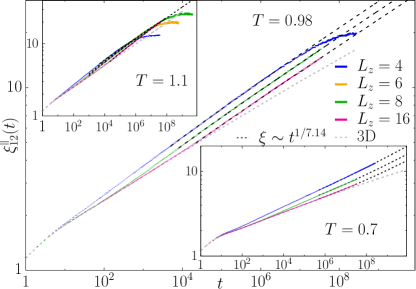
Figure 1: The longitudinal correlation length $\xi_{12}^{\parallel}(T,t)$, as computed in films of thickness $L_{z}$, versus the waiting time $t$ after a quench to temperature $T$, for $T=0.98$ (main), $T=1.1$ (upper inset) and $T=0.7$ (lower inset). The critical temperature is $T_{\mathrm{c}}=1.102(3)$ Baity-Jesi et al. (2013). As a reference, we also show purely 3D dynamics (data taken from Ref. Baity-Jesi et al. (2018)) and fits to 2D dynamics $\xi_{12}^{\parallel}(L_{z},T,t)\approx b(L_{z},T)\ +\ a(L_{z},T)t^{1/z_{\mathrm{2D}}}$, with $z_{\mathrm{2D}}=7.14\,$ Fernández et al. (2019) [fit parameters: $b(L_{z},T)$ and $a(L_{z},T)$].

Next, we compare $\xi^{\parallel}$ and $\xi^{\perp}$ in Fig. 2. The dynamical behaviors of these two quantities are very different. As expected $\xi^{\perp}$ saturates to a value near $L_{z}/2$ (which is the maximum value with PBC). However, $\xi^{\parallel}$ continues growing after $\xi^{\perp}$ saturates: in no way the time where $\xi^{\perp}$ and $\xi^{\parallel}$ stop growing is the same. In fact, $\xi_{12}^{\parallel}$ needs time to respond to the saturation of $\xi_{12}^{\perp}$: even the switch from the 3D like growth to the faster-than-3D growth arrives at a later time (see the inset in the $T=0.98$ part of Fig. 2). Saturation of $\xi^{\parallel}$ eventually happens, at later times. Although $\xi_{12}^{\parallel}$ saturates as well, these two time scales are remarkably different.

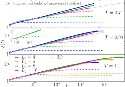
Figure 2: Growth of the longitudinal $\xi_{12}^{\parallel}$ (solid lines) and of the transversal $\xi_{12}^{\perp}$ (dashes lines) correlation lengths with the waiting time $t$ after a quench to temperature $T$. The inset (for $L_{z}=8$) is a zoom of the saturation of $\xi_{12}^{\perp}$ and of the separation between the $\xi_{12}^{\parallel}$ and the bulk correlation length (see the main text for more details).

In order to gain some understanding, we have identified a second characteristic length (besides the thickness $L_{z}$) that controls the 3D-to-2D crossover, namely the bulk correlation $\xi_{12}^{\mathrm{3D}}(t)$ Baity-Jesi et al. (2018). We have studied the behavior of the dimensionless $\xi_{12}^{\parallel}(t)/\xi_{12}^{\mathrm{3D}}(t)$ as a function of $\xi_{12}^{\mathrm{3D}}(t)/L_{z}$. In other words, we change variables from $t$ to $\xi_{12}^{\mathrm{3D}}(t)$. As one can see in Fig. 3 a very good scaling behavior emerges. This not only confirms the existence of the 3D-to-2D crossover, but also unveils some of its features. Indeed, the ratio $\xi_{12}^{\parallel}(t)/\xi_{12}^{\mathrm{3D}}(t)$ grows beyond 1, thus signaling a faster-than-3D dynamics as soon as $\xi_{12}^{\mathrm{3D}}(t)\approx L_{z}/4$ (for all our $T<T_{\mathrm{c}}$).

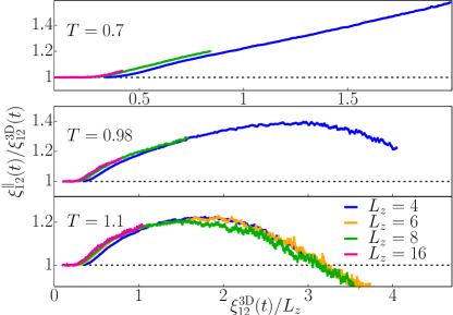
Figure 3: Dynamical scale-invariance for the dimensionless quantity $\xi_{12}^{\mathrm{film}}(t)/\xi_{12}^{\mathrm{3D}}(t)$ as a function of the rescaled bulk length $\xi_{12}^{\mathrm{3D}}(t)/L_{z}$.

The scale-invariance evinced in Fig. 3 prompts us to consider the film dynamics from the Renormalization-Group perspective (see e.g. Amit and Martín-Mayor (2005)). Indeed, in equilibrium, phenomenological renormalization Nightingale (1976) maps our film at temperature $T$ to a truly 2D spin glass at an effective temperature $T_{\text{eff,2D}}$ (for details, see below and appendix D):

$$\xi_{12}^{\parallel,\mathrm{eq}}\left(T,L_{z}\right)=L_{z}\,\xi_{12}^{\mathrm{eq,2D}}\left(T_{\text{eff,2D}}\right)\,,$$ (4)

where the equilibrium correlation length $\xi_{12}^{\mathrm{eq,2D}}$ is a smooth function of $T_{\text{eff,2D}}$ (provided that $T_{\text{eff,2D}}>0$). For any fixed $T>T_{\mathrm{c}}$, $T_{\text{eff,2D}}$ increases with $L_{z}$ ($T_{\text{eff,2D}}\to\infty$ when $L_{z}\to\infty)$. On the other hand, holding fixed $T\leq T_{\mathrm{c}}$ while $L_{z}$ grows, $T_{\text{eff,2D}}$ reaches a limit. The limit is neither $0$ nor $\infty$, because the whole spin-glass phase is critical in 3D Alvarez Baños et al. (2010); Contucci et al. (2009).

Two questions naturally appear: (i) Is the equilibrium mapping (4) meaningful for an aging, off-equilibrium film? and (ii) Is it sensible to assume $T_{\text{eff,2D}}\approx T$? (an assumption that, although not explictly, underlies the experimental analysis Guchhait and Orbach (2014, 2017); Zhai et al. (2017); Kenning et al. (2018)).

In order to address the above two questions, we perform on our aging films a linear Kadanoff-Wilson block spin transformation of size $L_{z}$ (see appendix D): from $L_{z}^{3}$ of our original spins at time $t$, we obtain a single renormalized spin in the renormalized 2D system. The correlation functions computed for the aging renormalized spins can be compared with those of a truly 2D system at the temperature $T_{\text{eff,2D}}$ obtained from Eq. (4). In particular, we have found it useful to compute the dimensionless ratio $\xi^{\text{RG}}_{23}(t)/\xi^{\text{RG}}_{12}(t)$ as computed from the block spins, see Fig. 4 (of course, for the truly 2D system, $L_{z}=1$, $\xi$ and $\xi^{\text{RG}}$ are the same quantity). This ratio is a smooth function of $\xi^{\text{RG}}_{12}(t)/\xi_{12}^{\text{RG,eq}}$  ].

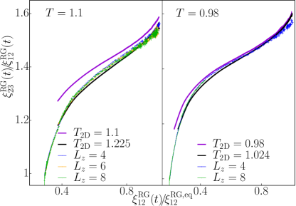
Figure 4: The scale-invariant ratio $\xi^{\text{RG}}_{23}(T,t)/\xi^{\text{RG}}_{12}(T,t)$, versus the ratio $\xi^{\text{RG}}_{12}(t,T)/\xi_{12}^{\mathrm{RG,eq}}(T)$ as computed from the block-spins [$\xi^{\text{RG}}_{12}(t,T)$ grows monotonically to its equilibrium value $\xi_{12}^{\mathrm{RG,eq}}(T)$]. For $T=1.1\approx T_{\mathrm{c}}$ and $T=0.98\approx 0.9T_{\mathrm{c}}$, we compare the scaling function obtained from block-spins (as extracted from films of several thickness $L_{z}$), with two analogous functions computed in purely 2D systems. If the 2D system is considered at the film’s temperature $T_{\text{2D}}=T$, the scaling function $\xi^{\text{2D}}_{23}(T,t)/\xi^{\text{2D}}_{12}(T,t)$ clearly differs from the block-spin result. On the other hand, the film and the 2D scaling function essentially coincide if the 2D system is considered at the effective temperature $T_{\text{eff,2D}}$ defined by Eq. (4).

As expected for a film at $T\leq T_{\mathrm{c}}$, the scaling function in Fig. 4 has no dependency in $L_{z}$. To be precise, for $T=0.98$ we did not reach equilibrium in the $L_{z}=8$ film. However, by taking $\xi_{12}^{\text{eq}}$ from the block-spins formed from the $L_{z}=4$ film, we find an excellent scaling: corrections to scaling, if any, are not measurable within our statistical accuracy for the films.

Now, the very same scaling function can be computed in a truly 2D system at temperature $T_{\text{2D}}$. If one takes $T_{\text{2D}}=T$ ($T$ is the film’s temperature), we find a clear discrepancy in Fig. 4 . On the other hand, if we take $T_{\text{2D}}=T_{\text{eff,2D}}$ the matching with the film’s scaling function is much better, in spite of the fact that corrections to scaling for the 2D system are suppressed only when $T_{\text{2D}}\to 0$ Fernandez et al. (2016). Hence, the answer to our first question above is yes, Eq. (4) is meaningful in the off-equilibrium regime, as well.

As for our second question, Finite Size Scaling (see e.g. Amit and Martín-Mayor (2005)) implies $\mathrm{d}T_{\text{eff,2D}}/\mathrm{d}T\propto L_{z}^{1/\nu}$ at $T_{\mathrm{c}}$. Hence, when $L_{z}$ grows, the mapping $T\to T_{\text{eff,2D}}$ becomes singular at $T=T_{\mathrm{c}}$. On the other hand, we do not see questions of principle implying a singular mapping for $T<T_{\mathrm{c}}$. Accordingly, we find $T_{\text{eff,2D}}\approx 1.11T$ at $T=T_{\mathrm{c}}$, but $T_{\text{eff,2D}}\approx 1.04T$ at $T\approx 0.9T_{\mathrm{c}}$. In other words, the assumption $T_{\text{eff,2D}}\approx T$ is sensible, provide that $T<T_{\mathrm{c}}$.

V Conclusions

Recent experiments in films Guchhait and Orbach (2014, 2017); Zhai et al. (2017); Kenning et al. (2018) focused on the saturation time, when the spin-glass correlation length $\xi$ no longer grows due to the dimensional crossover. From Eq. (4) and Figs. 4 and 3, we expect for this saturation time

$$t_{\text{sat}}(L_{z},T)\approx t_{\text{3D}}(L_{z},T)\,\varphi(\xi_{12}^{\mathrm{eq,2D}})\,\tau^{\text{2D}}_{\text{eq}}(T_{\text{eff,2D}})\,,$$ (5)

where $t_{\text{3D}}(L_{z},T)$ is the time that a bulk, 3D system needs to reach $\xi^{\text{3D}}_{12}=L_{z}$ at temperature $T$, $\varphi$ is a smooth function and $\xi_{12}^{\mathrm{eq,2D}}$ is the correlation length of the effective 2D system (4). Hence, $t_{\text{sat}}$ is the product of the renormalized time-unit $t_{\text{3D}}(L_{z},T)\,\varphi(\xi_{12}^{\mathrm{eq,2D}})$, times $\tau^{\text{2D}}_{\text{eq}}$ (i.e. the number of time-units that a $2D$ system needs to equilibrate at the effective temperature $T_{\text{eff,2D}}$). Experiments Guchhait and Orbach (2014, 2017); Zhai et al. (2017); Kenning et al. (2018) aim to extract the aging rate (1), which depends on $t_{\text{3D}}$ and $\xi_{\text{3D}}$, but they actually measure $t_{\text{sat}}$ and $L_{z}$. Nevertheless, we conclude that the experimental determination of the aging rate is safe, thanks to three fortunate facts: (i) $T_{\text{eff,2D}}\approx T$ below $T_{\mathrm{c}}$, (ii) the factor $\varphi(\xi_{12}^{\mathrm{eq,2D}})$ depends only on temperature (and very mildly so, see Fig. 3) and (iii) the growth of $\tau^{\text{2D}}_{\text{eq}}$ is only slightly super-Arrhenius (the aging rate is blind to Arrhenius time-growth).

We remark as well that there is more than the saturation time in film dynamics (we have identified four separate regimes). The exploration of this rich behavior opens an opportunity window for the fruitful interaction of experimental and numerical work in spin glasses.

Appendix A Multispin coding

We have simulated the Metropolis dynamics through two different multispin codings: MUlti SAmple multispin coding (MUSA) and MUlti SIte multispin coding (MUSI) Fernández and Martín-Mayor (2015).

The MUSA algorithm is based on the representation of many sample systems in a single computer word (128 bits in our implementation), i.e. each bit represents a different sample; instead, the MUSI one represents many spins of the same replica in a single computer word (256 bits in our implementation). Indeed, the code implementing MUSA is much simpler and thus it was adequate for the first stages of the project. On the Intel(R) Xeon(R) E5-2680v3 processors of the Cierzo cluster, our MUSA code simulates 24 replicas of the same sample at a rate of 12 picoseconds per spin flip (performance is optimal with this configuration because the memory-consuming coupling matrix is shared by the 24 replicas). Furthermore, the efficiency of MUSA algorithm does not depend on the choice of boundary conditions, either Open or Periodic.

On the other hand, the MUSI code has longer development times, but is significantly faster than MUSA [the lower the temperature, the faster: MUSI codes update $\sim\exp(4/T)$ spins with a single random number Fernández and Martín-Mayor (2015)]. Indeed, at our highest temperature $T=1.1$, on the E5-2680v3 processors, our MUSI code simulates 24 replicas at an overall rate of 8 picoseconds per spin flip. Unfortunately, for open boundary conditions, spins on the top (or bottom) layer have only 5 neighbors, which implies that one can only update $\sim\exp(2/T)$ spins with a single random number. Hence, we have implemented MUSI only for periodic boundary conditions.

Appendix B Statistical errors, samples and replicas

We have computed $C_{4}\left(T,\bm{r},t\right)$ [see Eq. (2)] at times $t=\text{integer-part-of }2^{i/4}$. For the estimation of the integrals $I_{k}(T,t)$ [see Eq. (3)] we have followed the methods explained in Fernández et al. (2019).

After a time $t^{*}$ the correlation length $\xi_{12}^{\parallel}$ does not show any dependence of time, implying that thermal equilibrium has been reached (see Fig. 1). In the calculation of Eq. (2) at equilibrium there is no reason to take the two real replicas at the same time $t$ and we can gain statistics averaging over pairs of times $(t_{1},t_{2})$ both larger than the safe equilibration threshold time $t^{*}$.

The choice of the optimal number of replicas $N_{\mathrm{R}}$ and samples $N_{\mathrm{S}}$ was chosen in order to minimize the final errors of the correlation length $\xi_{12}^{\parallel}(t)$, given a fixed computer effort $E=N_{\mathrm{R}}N_{\mathrm{S}}$. Indeed, the variance (or squared error) in $\xi_{12}$ approximately follows this behavior in the off-equilibrium regime Baity-Jesi et al. (2018):

$$\varDelta(N_{\mathrm{S}},N_{\mathrm{R}})=\left[\sigma_{\mathrm{S}}^{2}+\sigma_{\mathrm{R}}^{2}\left(\frac{2}{N_{\mathrm{R}}(N_{\mathrm{R}}-1)}\right)^{x}\right]\frac{1}{N_{\mathrm{S}}}\,,$$ (6)

where the exponent $x$ takes a value in the range $0.5<x<1$, $\sigma_{\mathrm{S}}^{2}$ and $\sigma_{\mathrm{R}}^{2}$ are (respectively) the sample and thermal contributions to the variance and $N_{\mathrm{R}}(N_{\mathrm{R}}-1)/2$ is the number of distinct pairs of replica indices for calculating $C_{4}(\bm{r},t)$, see Eq. (2). Clearly, we need to find a compromise by minimizing the (squared) error achievable for a fixed numerical effort $E=N_{\mathrm{R}}N_{\mathrm{S}}$, which results into an optimal value

$$N_{\mathrm{R}}^{*}\approx\left[2^{x}(2x-1)\frac{\sigma_{\mathrm{R}}^{2}}{\sigma_{\mathrm{S}}^{2}}\right]^{1/(2x)}\,,$$ (7)

[the result is approximated because we simplified the algebra as $N_{\mathrm{R}}(N_{\mathrm{R}}-1)\approx N_{\mathrm{R}}^{2}$].

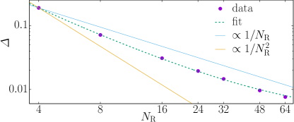
Figure 5: Squared statistical error for $\xi_{12}(T_{\mathrm{c}},t\!=\!2^{22},L_{z}\!=\!4)$, as computed from a set of $N_{\mathrm{S}}=128$ samples and $N_{\mathrm{R}}$ replicas, versus $N_{\mathrm{R}}$. The dashed line is a fit to Eq. (6). The relevant quantities extracted from the fit are $\sigma_{\mathrm{R}}^{2}/\sigma_{\mathrm{S}}^{2}\approx 156$ and $x\approx 0.65$. For reference, we show with continuous lines the two extremal behaviors, namely $x=1$ (with $\varDelta\propto 1/N_{\mathrm{R}}^{2}$) and $x=0.5$ (with $\varDelta\propto 1/N_{\mathrm{R}}$). Because $\sigma_{\mathrm{R}}^{2}\gg\sigma_{\mathrm{S}}^{2}$, $\varDelta$ shows an intermediate behavior for small $N_{\mathrm{R}}$. However, when $N_{\mathrm{R}}>30$ the contribution of thermal fluctuations to the final error becomes comparable to the sample contribution and there is little gain in further increasing $N_{\mathrm{R}}$.

At this point, we needed to estimate the ratio $\sigma_{\mathrm{R}}^{2}/\sigma_{\mathrm{S}}^{2}$, as well as the exponent $x$. In order to do so, we carried out short MUSI runs with $t=2^{22}$ at $T_{\mathrm{c}}$, for thickness $L_{z}=4$, with $N_{\mathrm{R}}^{\text{tot}}=72$ and $N_{\mathrm{S}}=128$. We randomly extracted $N_{\mathrm{R}}=4,8,16,24,32,48$ and $64$ replicas out of the ensemble of $N_{\mathrm{R}}^{\text{tot}}$ possibilities, and computed $\xi_{12}$ and its squared error $\varDelta(N_{\mathrm{S}},N_{\mathrm{R}})$ with the jackknife, see e.g. Ref. Amit and Martín-Mayor (2005) (we computed jackknife blocks over the samples). In order to stabilize the estimation of $\varDelta$ we averaged over 20 random extractions of the $N_{\mathrm{R}}$ replicas. The obtained $\varDelta(N_{\mathrm{R}},N_{\mathrm{S}})$ are shown in Fig. 5 with our fit to Eq. (6).

The resulting optimal value is $N_{\mathrm{R}}^{*}\approx 29.4$ [the approximation in Eq. (7) predicts 27.3]. However, by plugging $N_{\mathrm{S}}=E/N_{\mathrm{R}}$ in Eq. (6) and varying $N_{\mathrm{R}}$ while keeping $E$ fixed, we observed that the minimum at $N_{\mathrm{R}}^{*}$ is quite broad, which is fortunate because the value that optimizes the performance of our MUSA code on the Cierzo processors is $N_{\mathrm{R}}=24$.

Our final choices are as follows. With our (more flexible) MUSI code we simulated $N_{\mathrm{S}}=120$ independent samples, each with $N_{\mathrm{R}}=32$ replicas. In the MUSA case, we simulated 4 independent runs of 128 different samples and $N_{\mathrm{R}}=24$ real replicas. There is a caveat, though. The MUSA algorithm, sharing, by construction, the random numbers for all the samples in a computer word, could introduce some statistical correlation between different samples. We initially checked the statistical correlation comparing the error determination either assuming $N_{\mathrm{S}}=512$ independent samples or 4 independent blocks of 128 samples. Although with 4 sets the error determination is very imprecise, we found no significant signal of correlations. Furthermore, as soon as the MUSI algorithm was implemented, we checked carefully the real statistical sample independency by comparing the statistical errors for our observables as computed with the two algorithms. After this comparison, we found consistent the computation of errors under the hypothesis that the 512 samples in the four MUSA simulations are statistically independent. In fact, the independence hypothesis seems to systematically underestimate errors only for $C_{4}(r,t)$ at distance $r=1$, and (probably) for $r=2$ as well. The effect of this error underestimation can be observed in global magnitudes such as $\xi_{12}^{\parallel}$ only for very short times ($t<20$) when $\xi_{12}^{\parallel}$ itself is very small. Hence, we have decided to accept the independence hypothesis in our error computations for MUSA simulations.

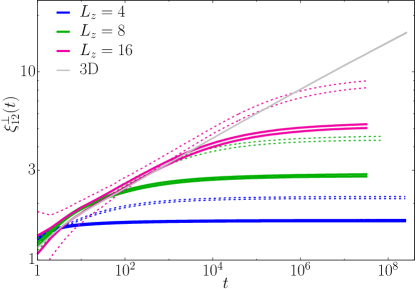
Figure 6: Growth of the transversal correlation length $\xi_{12}^{\perp}(T,t)$ at $T=0.98$ as function of the waiting time $t$ in scale log-log. The PBC (OBC) case is depicted in solid (dashed) lines.

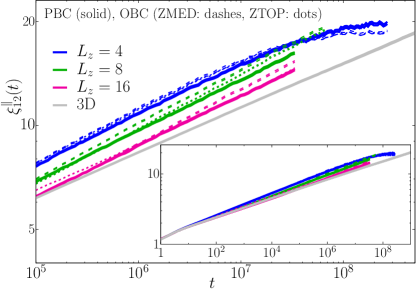
Figure 7: Growth of the longitudinal correlation length $\xi_{12}^{\parallel}(T,t)$ at $T=0.98$ as function of the waiting time $t$ as computed with periodic boundary conditions (PBC) or with open boundary conditions (OBC) on the central layer (ZMED) or on the top layer (ZTOP). The inset shows the data from the main panel in the full time-range of our simulations.

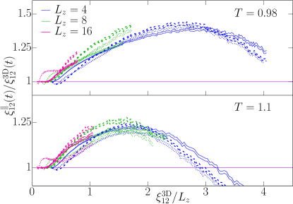
Figure 8: Dynamical scale-invariance for the dimensionless quantity $\xi_{12}^{\parallel}(t)/\xi_{12}^{\mathrm{3D}}(t)$ as a function of the rescaled bulk length $\xi_{12}^{\mathrm{3D}}(t)/L_{z}$, for the PBC case (solid), for the OBC central-layer (dashes) and for the OBC external-layer (dots) at temperatures $T=0.98$ (top) and $T=1.1$ (bottom).

Appendix C Boundary conditions

In the phenomenology of glassy films, the transversal saturation of $\xi_{12}^{\perp}$ activates the dimensional crossover and so, the boundary conditions could play a physical relevant role. In order to assess the effect of the boundary conditions, we carried out MUSA simulations with both Open (OBC) and Periodic Boundary Conditions (PBC) for several temperatures and $L_{z}$’s (recall that $L_{z}$ is the film thickness). Exploiting the same kind of analysis introduced in the main text, we found that our main results are not dependent on boundary conditions.

Regarding the sum estimator $\xi_{12}^{\perp}$ defined in Eq. (3), for OBC and computing the correlations from the bottom layer at $z\!=\!0$, we can extend the sum up to $L_{z}-1$. Hence, by construction, $\xi_{12}^{\perp}$ is larger for OBC than for PBC (see Fig.  6).

As for the comparison of the parallel dynamics, in the case of OBC we need to face the possibility of layer dependence. However, Fig. 7 tells us that the differences between $\xi_{12}^{\parallel}(T,t)$ as computed for the top layer and the central layer are tiny (and the difference with the PBC result is tiny as well), although our data are accurate enough to resolve the difference. In fact, see Fig. 8, the layer-dependence with OBC makes slightly more complicated the analysis of scaling functions.

Appendix D Renormalization Group

We decomposed our system in boxes of size of $L_{z}^{3}$ and we rescaled the overlap field as

$$Q^{(a,b)}(\bm{X},t)=\frac{1}{L_{z}^{3}}\sum_{r_{1},r_{2},r_{3}=0}^{L_{z}-1}q^{(a,b)}(\bm{r}+L_{z}\bm{X},t)\,,$$ (8)

and we defined the correlation function in the (2D) renormalized lattice as:

$$C_{4}^{\text{RG}}(T,\bm{R},t)=\overline{\langle Q^{(a,b)}(\bm{X},t)Q^{(a,b)}(\bm{X}+\bm{R},t)\rangle_{T}}\,.$$ (9)

We gain statistics by averaging over all the $L_{z}^{3}$ possible starting position of the boxes and all pairs of different replicas. The estimate of the correlation length was done as well through the integral estimators defined in the main text. Specifically, we computed the integrals

$$I^{\text{RG}}_{k}(T,t)=\int_{0}^{\infty}\mathrm{d}R\,R^{k}\,C_{4}^{\text{RG}}(T,R,t)\,,$$ (10)

and we estimated the correlation length as

$$\xi_{k,k+1}^{\text{RG}}(T,t)=I^{\text{RG}}_{k+1}(T,t)/I^{\text{RG}}_{k}(T,t)\,.$$ (11)

References

- Mézard et al. (1987) M. Mézard, G. Parisi, and M. Virasoro, Spin-Glass Theory and Beyond (World Scientific, Singapore, 1987).
- Fisher and Hertz (1991) K. Fisher and J. Hertz, Spin Glasses (Cambridge University Press, Cambridge England, 1991).
- Young (1998) A. P. Young, Spin Glasses and Random Fields (World Scientific, Singapore, 1998).
- Cugliandolo and Kurchan (1993) L. F. Cugliandolo and J. Kurchan, Phys. Rev. Lett. 71, 173 (1993).
- Franz et al. (1999) S. Franz, M. Mézard, G. Parisi, and L. Peliti, Journal of Statistical Physics 97, 459 (1999).
- Alvarez Baños et al. (2010) R. Alvarez Baños, A. Cruz, L. A. Fernandez, J. M. Gil-Narvion, A. Gordillo-Guerrero, M. Guidetti, A. Maiorano, F. Mantovani, E. Marinari, V. Martín-Mayor, J. Monforte-Garcia, A. Muñoz Sudupe, D. Navarro, G. Parisi, S. Perez-Gaviro, J. J. Ruiz-Lorenzo, S. F. Schifano, B. Seoane, A. Tarancon, R. Tripiccione, and D. Yllanes, (Janus Collaboration), Phys. Rev. Lett. 105, 177202 (2010) .
- Baity-Jesi et al. (2017a) M. Baity-Jesi, E. Calore, A. Cruz, L. A. Fernandez, J. M. Gil-Narvión, A. Gordillo-Guerrero, D. Iñiguez, A. Maiorano, E. Marinari, V. Martin-Mayor, J. Monforte-Garcia, A. Muñoz Sudupe, D. Navarro, G. Parisi, S. Perez-Gaviro, F. Ricci-Tersenghi, J. J. Ruiz-Lorenzo, S. F. Schifano, B. Seoane, A. Tarancón, R. Tripiccione, and D. Yllanes, Proceedings of the National Academy of Sciences 114, 1838 (2017a).
- Baity-Jesi et al. (2014) M. Baity-Jesi, R. A. Baños, A. Cruz, L. A. Fernandez, J. M. Gil-Narvion, A. Gordillo-Guerrero, D. Iniguez, A. Maiorano, F. Mantovani, E. Marinari, V. Martín-Mayor, J. Monforte-Garcia, A. Muñoz Sudupe, D. Navarro, G. Parisi, S. Perez-Gaviro, M. Pivanti, F. Ricci-Tersenghi, J. J. Ruiz-Lorenzo, S. F. Schifano, B. Seoane, A. Tarancon, R. Tripiccione, and D. Yllanes, (Janus Collaboration), Comp. Phys. Comm 185, 550 (2014) .
- Manssen and Hartmann (2015) M. Manssen and A. K. Hartmann, Phys. Rev. B 91, 174433 (2015) .
- Fernández and Martín-Mayor (2015) L. A. Fernández and V. Martín-Mayor, Phys. Rev. B 91, 174202 (2015).
- Belletti et al. (2008) F. Belletti, M. Cotallo, A. Cruz, L. A. Fernandez, A. Gordillo-Guerrero, M. Guidetti, A. Maiorano, F. Mantovani, E. Marinari, V. Martín-Mayor, A. M. Sudupe, D. Navarro, G. Parisi, S. Perez-Gaviro, J. J. Ruiz-Lorenzo, S. F. Schifano, D. Sciretti, A. Tarancon, R. Tripiccione, J. L. Velasco, and D. Yllanes, (Janus Collaboration), Phys. Rev. Lett. 101, 157201 (2008) .
- Belletti et al. (2009) F. Belletti, A. Cruz, L. A. Fernandez, A. Gordillo-Guerrero, M. Guidetti, A. Maiorano, F. Mantovani, E. Marinari, V. Martín-Mayor, J. Monforte, A. Muñoz Sudupe, D. Navarro, G. Parisi, S. Perez-Gaviro, J. J. Ruiz-Lorenzo, S. F. Schifano, D. Sciretti, A. Tarancon, R. Tripiccione, and D. Yllanes, (Janus Collaboration), J. Stat. Phys. 135, 1121 (2009) .
- Manssen et al. (2015) M. Manssen, A. K. Hartmann, and A. P. Young, Phys. Rev. B 91, 104430 (2015) .
- Baity-Jesi et al. (2017b) M. Baity-Jesi, E. Calore, A. Cruz, L. A. Fernandez, J. M. Gil-Narvion, A. Gordillo-Guerrero, D. Iñiguez, A. Maiorano, E. Marinari, V. Martin-Mayor, J. Monforte-Garcia, A. Muñoz-Sudupe, D. Navarro, G. Parisi, S. Perez-Gaviro, F. Ricci-Tersenghi, J. J. Ruiz-Lorenzo, S. F. Schifano, B. Seoane, A. Tarancon, R. Tripiccione, and D. Yllanes, (Janus Collaboration), Phys. Rev. Lett. 118, 157202 (2017b).
- Baity-Jesi et al. (2018) M. Baity-Jesi, E. Calore, A. Cruz, L. A. Fernandez, J. M. Gil-Narvion, A. Gordillo-Guerrero, D. Iñiguez, A. Maiorano, E. Marinari, V. Martin-Mayor, J. Moreno-Gordo, A. Muñoz-Sudupe, D. Navarro, G. Parisi, S. Perez-Gaviro, F. Ricci-Tersenghi, J. J. Ruiz-Lorenzo, S. F. Schifano, B. Seoane, A. Tarancon, R. Tripiccione, and D. Yllanes, (Janus Collaboration), Phys. Rev. Lett. 120, 267203 (2018).
- Fernández et al. (2019) L. A. Fernández, E. Marinari, V. Martín-Mayor, G. Parisi, and J. Ruiz-Lorenzo, Journal of Physics A: Mathematical and Theoretical 52, 224002 (2019).
- Fernández et al. (2018) L. A. Fernández, E. Marinari, V. Martín-Mayor, G. Parisi, and J. Ruiz-Lorenzo, Journal of Statistical Mechanics: Theory and Experiment 2018, 103301 (2018) .
- Joh et al. (1999) Y. G. Joh, R. Orbach, G. G. Wood, J. Hammann, and E. Vincent, Phys. Rev. Lett. 82, 438 (1999).
- Guchhait and Orbach (2014) S. Guchhait and R. Orbach, Phys. Rev. Lett. 112, 126401 (2014).
- Guchhait and Orbach (2017) S. Guchhait and R. L. Orbach, Phys. Rev. Lett. 118, 157203 (2017).
- Zhai et al. (2017) Q. Zhai, D. C. Harrison, D. Tennant, E. D. Dahlberg, G. G. Kenning, and R. L. Orbach, Phys. Rev. B 95, 054304 (2017).
- Kenning et al. (2018) G. G. Kenning, D. M. Tennant, C. M. Rost, F. G. da Silva, B. J. Walters, Q. Zhai, D. C. Harrison, E. D. Dahlberg, and R. L. Orbach, Phys. Rev. B 98, 104436 (2018).
- Bray et al. (1986) A. J. Bray, M. A. Moore, and A. P. Young, Phys. Rev. Lett. 56, 2641 (1986).
- Franz et al. (1994) S. Franz, G. Parisi, and M. Virasoro, J. Phys. (France) 4, 1657 (1994).
- Maiorano and Parisi (2018) A. Maiorano and G. Parisi, Proceedings of the National Academy of Sciences 115, 5129 (2018) .
- Note (1) At the critical temperature , the aging rate coincides with the so-called dynamic critical exponent.
- Bert et al. (2004) F. Bert, V. Dupuis, E. Vincent, J. Hammann, and J.-P. Bouchaud, Phys. Rev. Lett. 92, 167203 (2004).
- Nightingale (1976) M. Nightingale, Physica A: Statistical Mechanics and its Applications 83, 561 (1976).
- Gunnarsson et al. (1991) K. Gunnarsson, P. Svedlindh, P. Nordblad, L. Lundgren, H. Aruga, and A. Ito, Phys. Rev. B 43, 8199 (1991).
- Palassini and Caracciolo (1999) M. Palassini and S. Caracciolo, Phys. Rev. Lett. 82, 5128 (1999) .
- Ballesteros et al. (2000) H. G. Ballesteros, A. Cruz, L. A. Fernandez, V. Martín-Mayor, J. Pech, J. J. Ruiz-Lorenzo, A. Tarancon, P. Tellez, C. L. Ullod, and C. Ungil, Phys. Rev. B 62, 14237 (2000) .
- Fernández et al. (2016) L. A. Fernández, E. Marinari, V. Martín-Mayor, G. Parisi, and D. Yllanes, Journal of Statistical Mechanics: Theory and Experiment 2016, 123301 (2016) .
- Khoshbakht and Weigel (2018) H. Khoshbakht and M. Weigel, Phys. Rev. B 97, 064410 (2018).
- Edwards and Anderson (1975) S. F. Edwards and P. W. Anderson, Journal of Physics F: Metal Physics 5, 965 (1975).
- sup (2019)
- Mydosh (1993) J. A. Mydosh, Spin Glasses: an Experimental Introduction (Taylor and Francis, London, 1993).
- Parisi (1988) G. Parisi, Statistical Field Theory (Addison-Wesley, 1988).
- Note (2) A Renormalization Group argument implies that the scaling function depends as well on the effective two-dimensional temperature , see Eq. (4\@@italiccorr). In equilibrium, decays for large as Fernández et al. (2018) ( is reachable in a film at only thanks to the 3D-to-2D crossover Guchhait and Orbach (2014)). Off-equilibrium, decays super-exponentially in Fernández et al. (2018).
- Baity-Jesi et al. (2013) M. Baity-Jesi, R. A. Baños, A. Cruz, L. A. Fernandez, J. M. Gil-Narvion, A. Gordillo-Guerrero, D. Iniguez, A. Maiorano, F. Mantovani, E. Marinari, V. Martín-Mayor, J. Monforte-Garcia, A. Muñoz Sudupe, D. Navarro, G. Parisi, S. Perez-Gaviro, M. Pivanti, F. Ricci-Tersenghi, J. J. Ruiz-Lorenzo, S. F. Schifano, B. Seoane, A. Tarancon, R. Tripiccione, and D. Yllanes, (Janus Collaboration), Phys. Rev. B 88, 224416 (2013) .
- Amit and Martín-Mayor (2005) D. J. Amit and V. Martín-Mayor, Field Theory, the Renormalization Group and Critical Phenomena, 3rd ed. (World Scientific, Singapore, 2005).
- Contucci et al. (2009) P. Contucci, C. Giardinà, C. Giberti, G. Parisi, and C. Vernia, Phys. Rev. Lett 103, 017201 (2009) .
- Note (3) We use as a computable proxy for the unknown in Eq. (2\@@italiccorr), see Fig. 4 and Ref. Fernández et al. (2018).
- Note (4) The reader migt be puzzled because all curves with in Fig. 4 were obtained at the film’s temperature . Indeed, by taking the limit , one could (wrongly) conclude . The way out of the paradox is, actually, one of the crucial ideas from the Renormalization Group Amit and Martín-Mayor (2005): although the film gets mapped into a 2D spin glass, the corresponding 2D model is certainly not as simple as ours (square lattice, nearest-neighbors interaction, couplings ). Phenomenological renormalization (PR) Nightingale (1976) was invented, precisely, to keep using the simplified model at the prize of changing parameters such as temperature, hence the need for the from Eq. (4\@@italiccorr). PR becomes exact only if (rather than ).
- Fernandez et al. (2016) L. A. Fernandez, E. Marinari, V. Martin-Mayor, G. Parisi, and J. J. Ruiz-Lorenzo, Phys. Rev. B 94, 024402 (2016).