Detection of the self-regulation of star formation in galaxy discs

Abstract

Stellar feedback has a notable influence on the formation and evolution of galaxies. However, direct observational evidence is scarce. We have performed stellar population analysis using MUSE optical spectra of the spiral galaxy NGC 628 and find that current maximum star formation in spatially resolved regions is regulated according to the level of star formation in the recent past. We propose a model based on the self-regulator or “bathtub” models, but for spatially resolved regions of the galaxy. We name it the “resolved self-regulator model” and show that the predictions of this model are in agreement with the presented observations. We observe star formation self-regulation and estimate the mass-loading factor, $\eta=2.5\pm 0.5$, consistent with values predicted by galaxy formation models. The method described here will help provide better constraints on those models.

1 Introduction

Stellar feedback is commonly invoked to reproduce observed galaxy properties in cosmologically based galaxy formation models (Hopkins et al., 2014; Vogelsberger et al., 2014; Schaye et al., 2015). Theory supports stellar feedback as the main mechanism which regulates the star formation in low mass galaxies, while active galactic nuclear (AGN) feedback is predicted to quench star formation in massive galaxies (Silk & Mamon, 2012). However, direct observational evidence supporting the stellar feedback scenario is lacking. Indirect evidence is based on the measurement of galaxy outflows (Bouche et al., 2012; Kacprzak et al., 2014; Schroetter et al., 2015; Lopez-Coba et al., 2018; Bik et al., 2018) or on analysing the chemical evolution of galaxies (Zhu et al., 2017) rather than measuring directly the self regulation of star formation.

The measurement of stellar feedback is critical in the reconciliation of the observed properties of galaxies with those from standard galaxy formation models (Hopkins et al., 2014; Vogelsberger et al., 2014; Schaye et al., 2015), and it is of great relevance in the stellar halo accretion rate efficiency (Rodrıguez-Puebla et al., 2016), particularly in low mass galaxies. Unfortunately, estimates of the stellar feedback, are scarce and depend on the observability and uncertain mass of galactic winds (Bouche et al., 2012; Kacprzak et al., 2014; Schroetter et al., 2015).

Very recently, using star formation histories SFHs derived from stellar population analysis the AGN regulated star formation has been inferred, through the connection between star formation and black hole mass in massive galaxies (Martın-Navarro et al., 2018). The same technique can be used to find a connection between the star formation at a given time, and star formation in the recent past. Although black hole activity is concentrated in the centre, it is capable of quenching star formation on galactic scales (Di Matteo et al., 2005). Star formation activity, however, although extended across the entire galaxy, produces its effects only close to its occurrence in space and time.

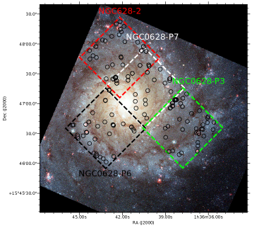
Figure 1: Colour composite image from HST with $1\rm{arcmin}\times 1\rm{arcmin}$ MUSE FOV overplotted. There are 4 pointings. We label them with their ESO archive labels. We also plot the compact star clusters centered regions as black circles.

If we want to measure the effects of stellar feedback, we must focus on time and spatial scales smaller than those affected by black hole feedback in massive galaxies, which is why we focus here on looking for the past stellar feedback in spatially resolved regions in the galaxy NGC 628 using optical spectra. NGC 628 is an almost face-on, grand design spiral galaxy, with a $\rm{SFR}=0.15\thinspace\rm{M_{\odot}/yr}$ and a total stellar mass of $M_{*}=1.2\times 10^{10}\thinspace\rm{M_{\odot}}$ (Zaragoza-Cardiel et al., 2018), right on the main sequence of star formation. NGC 628 has a disc-like pseudobulge (Zou et al., 2011), which helps us in the interpretation of the SFHs since the formation of the disc and the pseudobulge are both via secular evolution. The study would hardly be affected by the presence of a classical bulge since this would be made of stars older than the scale of ages we analyse.

We present the observational data and the stellar population synthesis analysis in section §2, while we propose a resolved self-regulation model of star formation in section §3. We compare the model with the observations in section §4. Finally, we present our conclusions in section §5.

2 Observational data & Stellar population synthesis analysis

We use data of NGC 628 from the Multi Unit Spectroscopic Explorer (MUSE) (Bacon et al., 2010) mounted on the Very Large Telescope (VLT). The data were downloaded from the ESO archive. MUSE in its wide field mode is an integral field spectrograph of $1\rm{arcmin}\times 1\rm{arcmin}$ field of view (FOV), with 2.6 Å spectral resolution, seeing limited angular resolution, and it has a spectral range between 4750 and 9350 Å.

We used the pointings of NGC 628 shown in Fig. 1: NGC0628-P3 (green square), NGC0628-P6 (black square), NGC0628-P7 (white square), and NGC628-2 (red square), with exposure times between $2350\rm{s}$ and $2780\rm{s}$. We have used the publicly available flux and wavelength calibrated datacubes (Kreckel et al., 2016; Kreckel et al., 2017, 2018). NGC628-2 and NGC0628-P7 pointings overlap significantly, so we use the data only from the NGC628-2 pointing where there is no overlap with NGC0628-P7.

In order to analyse the star formation regulation on different spatial scales, we divide each pointing into 9, 36, and 144 square regions, which results in 830, 415, and 207 pc-wide squares, respectively, as well as use circular regions of radius 87pc (black circles in Fig. 1), centred on compact star clusters identified as described in Santiago-Cortés et al. (2010) using HST data (Lomelí-Núñez et al. in preparation).

After we extract the spectrum for each individual region, we correct it for Galactic extinction and mask the foreground stars. We fit the stellar continuum and the emission lines of these spectra using the SINOPSIS code (Fritz et al., 2007, 2017). SINOPSIS estimates the combination of single stellar population (SSP) models which best fits the equivalent widths of the absorption and emission lines, and the stellar continuum in defined bands.

We do not assume any prior for the form of the SFH, allowing for a free form SFH. We use the Calzetti dust attenuation law (Calzetti et al., 2000), and the Chabrier 2003 IMF (Chabrier, 2003) with stellar mass limits between $0.15\rm{M_{\odot}}$ and $120\rm{M_{\odot}}$.

We use the updated version of the Bruzual & Charlot models described in Werle et al. (2019). We use SSP models for 3 metallicities ($Z=0.004$, $Z=0.02$, and $Z=0.04$) in 12 age bins (2 Myr, 4 Myr, 7 Myr, 20 Myr, 57 Myr, 200 Myr, 570 Myr, 1 Gyr, 3 Gyr, 5.75 Gyr, 10 Gyr, and 14 Gyr). The emission lines are computed for the SSPs younger than 20 Myr (Fritz et al., 2017) using the photoionisation code Cloudy (Ferland, 1993; Ferland et al., 1998; Ferland et al., 2013), assuming case B recombination (Osterbrock, 1989), an electron temperature of $10^{4}\rm{K}$, an electron density of $100\rm{cm}^{-3}$, and a gas cloud with an inner radius of $10^{-2}\rm{pc}$.

SINOPSIS fits the H$\alpha$ and H$\beta$ equivalent width estimates and the continuum in specific given bands. The continuum bands are chosen to be unaffected by sky subtraction effects, specially in the red part of the spectrum.

The degeneracies between age, metallicity, and dust attenuation, are used by the SINOPSIS code to estimate the uncertainties in the derived parameters (Fritz et al., 2007).

We bin the SFH in four age bins, $20\rm{Myr}$, $570\rm{Myr}$, $5.7\rm{Gyr}$, and $14\rm{Gyr}$, and analyse the two most recent star formation events. Removing the two oldest bins in our analysis improves the confidence in our results, since they are worse constrained than the more recent bins. We also choose to be conservative, characterising the SFH in the last 570 Myr in the simplest way, by using only two age bins. The SINOPSIS code has been tested with simulated and observed spectra (Fritz et al., 2007, 2011). SINOPSIS and similar codes have proved the validity of the use of SSP synthesis to extract non parametric SFHs in, at least, four age bins (Cid Fernandes et al., 2005; Fritz et al., 2007, 2011; Sánchez et al., 2016).

We have restricted the analysis to a main sequence star forming disc galaxy, which has evolved through secular evolution in the studied time range (last 570 Myr).

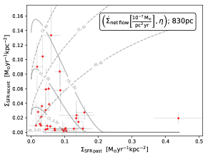
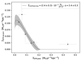
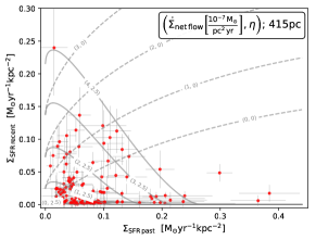
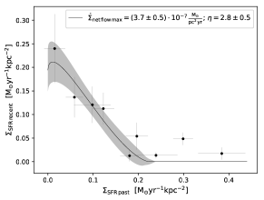
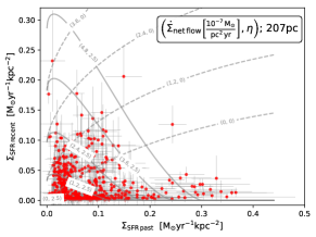
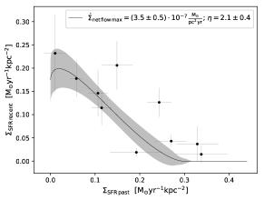
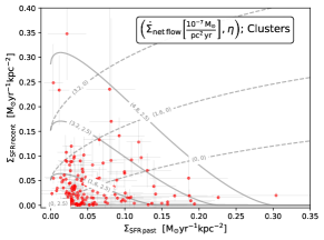
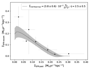
Figure 2: (a) SFR surface density in the 20 Myr age bin, $\Sigma_{\rm{SFR\thinspace recent}}$, versus SFR surface density in the 570 Myr age bin, $\Sigma_{\rm{SFR\thinspace past}}$ (red dots). The proposed resolved self regulator model values (Eq. 6) are plotted for several values of $\dot{\Sigma}_{\rm{net\thinspace flow}}$, and $\eta$ as solid ($\eta=2.5$) and dashed ($\eta=0$) grey lines. Each individual dot is for 830 pc-wide regions. (b) SFR surface density in the 20 Myr age bin, $\Sigma_{\rm{SFR\thinspace recent}}$, versus SFR surface density in the 570 Myr age bin, $\Sigma_{\rm{SFR\thinspace past}}$, for those regions closest to maximum $\dot{\Sigma}_{\rm{net\thinspace flow}}$ (upper envelope). The solid line is the fit of Eq. 6 to the envelope, where also we plot the 1-$\sigma$ uncertainty range of the fit as shadow regions. Each individual dot is for an 830 pc-wide region. (c) Panel is the same as (a) but for 415 pc-wide regions. (d) Panel is the same as (b) but for 415 pc-wide regions. (e) Panel is the same as (a) but for 415 pc-wide regions. (f) Panel is the same as (b) but for 415 pc-wide regions. (g) Panel is the same as (a) but for circles of radius 87 pc and centred on star clusters. (h) Panel is the same as (b) but for circles of radius 87 pc and centred on star clusters.

We extract the SFHs of each of the 207, 415, 830 pc-wide regions, as well as those centered in the star clusers in four age bins. We analyse the current ($20\rm{Myr}$), and the recent past ($570\rm{Myr}$) SFHs bins, in order to check if they correlate, i. e., if the current SFR is regulated by that in the recent past. For simplicity, we will refer to the recent past SFR (570 Myr age bin) as past SFR.

We compare the past SFR surface density, $\Sigma_{\rm{SFR\thinspace past}}$, with the recent SFR surface density (20 Myr age bin), $\Sigma_{\rm{SFR\thinspace recent}}$ in Fig. 2 (a, c, e, and (g)) for the different region sizes as red dots.

Although we do not, strictly, observe a correlation between past and present SFR surface densities, we do find in Fig. 2 (a, c, e, and (g)) that for all the analysed scales, the maximum $\Sigma_{\rm{SFR\thinspace recent}}$ compared to the $\Sigma_{\rm{SFR\thinspace past}}$ is determined by the level of $\Sigma_{\rm{SFR\thinspace past}}$. Regions where $\Sigma_{\rm{SFR\thinspace past}}$ was the highest do not present $\Sigma_{\rm{SFR\thinspace recent}}$ as high as those with less $\Sigma_{\rm{SFR\thinspace past}}$, and viceversa, regions where $\Sigma_{\rm{SFR\thinspace recent}}$ is the highest, did not have $\Sigma_{\rm{SFR\thinspace past}}$ as high as those with less $\Sigma_{\rm{SFR\thinspace recent}}$. This can be explained, at least qualitatively, if the maximum current SFR in a region is regulated by the SFR in the recent past.

3 Resolved self-regulation star formation model

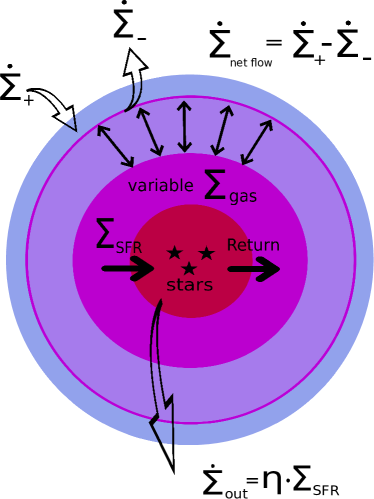
Figure 3: Resolved self-regulator model for a star forming region. The different layers within the circles refer to different components. The stellar disc and the star forming region are co-rotating. Invoking mass conservation, this model relates $\dot{\Sigma}_{\rm{gas}}$, $\dot{\Sigma}_{\rm{net\thinspace flow}}$, $\dot{\Sigma}_{\rm{out}}$, and $\Sigma_{\rm{SFR}}$.

In order to explain the observed star formation regulation, we propose a model based on the simplest models of star formation within galaxy evolution: the self-regulator or “bathtub” models (Bouche et al., 2010; Lilly et al., 2013; Peng & Maiolino, 2014; Dekel & Mandelker, 2014; Forbes et al., 2014; Ascasibar et al., 2015). Briefly, these models assume mass conservation and relate, for a whole galaxy , the change in time of the gas mass, $\dot{M}_{\rm{gas}}$, with the star formation rate, $\rm{SFR}$, the gas outflow rate, $\dot{M}_{\rm{out}}$, and the gas inflow rate, $\dot{M}_{\rm{in}}$:

$$\dot{M}_{\rm{gas}}={\dot{M}}_{\rm{in}}-{\rm{SFR}}(1-R+\eta)$$ (1)

where $R$ is the fraction of the mass that is returned to the interstellar medium, and $\eta$ is the “mass loading factor”,

$${\dot{M}}_{\rm{out}}=\eta{\rm{SFR}}.$$ (2)

A resolved self-regulator model of the ISM has been already proposed (Burkert, 2017). Based on the idea of a resolved version of the self-regulator models, we propose here one which is shown in the Fig. 3. The model relates, assuming mass conservation, the change in time of the gas mass surface density, $\dot{\Sigma}_{\rm{gas}}$, to the SFR surface density, ${\Sigma_{\rm{SFR}}}$, the net gas flow rate surface density, $\dot{\Sigma}_{\rm{net\thinspace flow}}$, and the gas outflow rate (due to stellar feedback) surface density, $\dot{\Sigma}_{\rm{out}}$:

$$\dot{\Sigma}_{\rm{gas}}={\dot{\Sigma}}_{\rm{net\thinspace flow}}-{\Sigma_{\rm{SFR}}}(1-R+\eta)$$ (3)

where

$${\dot{\Sigma}}_{\rm{out}}=\eta{\Sigma_{\rm{SFR}}}.$$ (4)

The resolved self-regulator proposed here is for an individual star or a group of stars which moves together through the rotation of the galaxy disc such as a massive star cluster ($>500\rm{M_{\odot}}$ Lada & Lada (2003)) . Thus, Eqs. 3 and 4 are defined locally, and the mass-loading factor is representative of massive star cluster scales ($\sim$pc Lada & Lada (2003)). The gas behaves as a collisional fluid, so we cannot assume that the gas follows the same rotation as the stars. For this reason we allow the gas to flow into and out of the region. We assume that these general flows are independent of any star formation inside the region, and that they depend on factors external to the region itself. The $\dot{\Sigma}_{\rm{net\thinspace flow}}$ term is defined as the difference between the gas surface density rate that enters the region, $\dot{\Sigma}_{+}$, minus the gas surface density rate that leaves the region, $\dot{\Sigma}_{-}$. Finally, the gas that flows out of the region due to stellar feedback is quantified by the ${\dot{\Sigma}}_{\rm{out}}$ term and represents the part of the gas that flows out which depends on the star formation within the region.

We assume that large regions,such as the ones observed in this study, are a sum of individual star forming regions that obey Eq. 3 for a specific time interval. This means that star forming regions that produce unbound star clusters are split into individual stars, and star forming regions that produce bound clusters where the feedback is thought to be more important and more connected with the region properties, can be considered as a whole. We do not consider the effect of feedback between regions, but only inside each region. We apply Eq. 3 to a sum of star forming regions that we observe as a larger one at the present time:

$$\dot{\overline{{\Sigma}}}_{\rm{gas}}=\dot{\overline{{\Sigma}}}_{\rm{net\thinspace flow}}-\overline{\Sigma}_{\rm{SFR}}(1-R+\eta)$$ (5)

where the average is done in the whole region we observe. We can derive or approximate the average quantities from the observations reported in the previous section. We have measured the $\overline{\Sigma}_{\rm{SFR\thinspace past}}$, as the sum of individual star forming regions that are affecting the present measured $\overline{\Sigma}_{\rm{SFR\thinspace recent}}$. We convert $\dot{\overline{{\Sigma}}}_{\rm{gas}}$ into $\frac{\overline{\Sigma}_{\rm{SFR\thinspace recent}}-\overline{\Sigma}_{\rm{SFR\thinspace past}}}{\Delta t}$. We rewrite Eq. 5 assuming that the $\Sigma_{\rm{SFR}}$ and the $\Sigma_{\rm{gas}}$ are related by the Kennicutt-Schmidt (KS) law (Kennicutt, 1998), $\Sigma_{\rm{SFR}}=A\Sigma_{\rm{gas}}^{N}$:

$$\begin{split}&\overline{\Sigma}_{\rm{SFR\thinspace recent}}=\\ &A\left\{\left[\dot{\overline{\Sigma}}_{\rm{net\thinspace flow}}-\overline{\Sigma}_{\rm{SFR\thinspace past}}\left(1-R+\eta\right)\right]\Delta t+\left[\frac{\overline{\Sigma}_{\rm{SFR\thinspace past}}}{A}\right]^{\frac{1}{N}}\right\}^{N}.\end{split}$$ (6)

Eq. 6, hence, relates the recent $\overline{\Sigma}_{\rm{SFR\thinspace recent}}$ with the past $\overline{\Sigma}_{\rm{SFR\thinspace past}}$, in terms of the mass loading factor, $\eta$, net gas flow rate surface density, $\dot{\overline{\Sigma}}_{\rm{net\thinspace flow}}$, the returned mass fraction, $R$, and the constants from the KS law, $A$, and $N$. We assume the instantaneous recycling approximation (Madau & Dickinson, 2014) for stars more massive than $3\rm{M_{\odot}}$ ($\tau_{\rm{MS}}\sim 0.6\rm{Gyr}$), a Chabrier IMF (Chabrier, 2003), and obtain a value of $R=0.27$.

Deviations from the instantaneous recycling approximation, such as considering gas recycle from stars more massive than $1\rm{M_{\odot}}$ ($\tau_{\rm{MS}}\sim 10\rm{Gyr}$) or stars more massive than $4\rm{M_{\odot}}$ ($\tau_{\rm{MS}}\sim 0.3\rm{Gyr}$) adds an error of $\pm 0.1$ in the considered value of $R$, which is a second order correction to the reported $\eta$ values. Recycling gas from stars less massive than $1\rm{M_{\odot}}$ is negligible since their life times on main sequence are similar to or larger than the Hubble time.

We also assume, $A=-4.32$, and $N=1.56$ (Kennicutt et al., 2007). The gas which regulates the SFR is molecular and atomic gas, and hence the choice of $A$ and $N$ (Kennicutt et al., 2007). This resolved self regulator model relates the gas inflow into the galaxy, mainly atomic gas, with that which is forming stars, mainly molecular gas. The two chosen ages for the recent and past age bins we used in our analysis are 20 Myr, and 570 Myr, respectively, so $\Delta t=550\thinspace\rm{Myr}$.

4 Comparison between the self-regulator model and the observations

We overplot in Fig. 2 (a, c, e and g) the theoretical relation between the past and recent SFR surface densities assuming the resolved self regulator model (Eq. 6) for a range of values of $\dot{\overline{\Sigma}}_{\rm{net\thinspace flow}}$ and $\eta$. It is clear that the effect of increasing ${\dot{\overline{\Sigma}}}_{\rm{net\thinspace flow}}$ is to increase the recent SFR surface density, while the effect of $\eta$, is to reduce the recent SFR surface density in proportion to the SFR surface density in the past.

The case of no self-regulation ($\eta=0$) is not favoured by the combination of the model and observations presented here, since the $\eta=0$ case plotted as dashed grey lines in Fig. 2 show that the most intense star forming regions in the past, would not have as much ${\dot{\overline{\Sigma}}}_{\rm{net\thinspace flow}}$ as the less intense star forming regions in the past. There are no realistic mechanisms in the resolved self-regulator model that could produce larger net gas rate inflows into regions where there was not much star formation.

For each different spatial scale, we can group the regions by their relative positions within the resolved self regulator model family as a function of $\dot{\overline{\Sigma}}_{\rm{net\thinspace flow}}$ (solid lines in Fig. 2 a, c, e and g). We identify a group of regions closer to the model curve where $\dot{\overline{\Sigma}}_{\rm{net\thinspace flow}}$ is maximum. We define empirically those regions close to the curve where $\dot{\overline{\Sigma}}_{\rm{net\thinspace flow}}$ is maximum as those with maximum $\overline{\Sigma}_{\rm{SFR\thinspace recent}}$ per bin of $\overline{\Sigma}_{\rm{SFR\thinspace past}}$. We call this group of regions the upper envelope and plot them as black dots in Fig. 2 (b, d, f, and h) for the different region sizes.

Assuming stochasticity on $\dot{\overline{\Sigma}}_{\rm{net\thinspace flow}}$ inside the regions, the data are compatible with the resolved self-regulator star formation model with random flows inside a range, $\dot{\overline{\Sigma}}_{\rm{net\thinspace flow}}\in[\dot{\overline{\Sigma}}_{\rm{net\thinspace flow\thinspace min}},\dot{\overline{\Sigma}}_{\rm{net\thinspace flow\thinspace max}}]$. Although the value of $\dot{\overline{\Sigma}}_{\rm{net\thinspace flow}}$ could be negative, we can not distinguish between negative and zero $\dot{\overline{\Sigma}}_{\rm{net\thinspace flow}}$ since the effect of negative and zero net flow is the same, to quench the recent star formation.

However, since there should exist a maximum net gas flow, $\dot{\overline{\Sigma}}_{\rm{net\thinspace flow\thinspace max}}$, there is a limit on the observed $\overline{\Sigma}_{\rm{SFR\thinspace recent}}$. Assuming that in a normal star forming main sequence spiral galaxy like NGC 628, there are a few regions where in 550Myr their net gas flow is approximately $\dot{\overline{\Sigma}}_{\rm{net\thinspace flow\thinspace max}}$, we can approximate those regions as those identified on the upper envelope.

Table 1: Resolved self-regulator model (Eq. 6) fit results. The fits are done to the regions on the upper envelope (plotted as black dots in Figs. 2 b, d, f, and h), which we interpret as region where $\dot{\overline{\Sigma}}_{\rm{net\thinspace flow\thinspace}}\approx\dot{\overline{\Sigma}}_{\rm{net\thinspace flow\thinspace max}}$

Region size (pc)	$\dot{\overline{\Sigma}}_{\rm{flow\thinspace max}}$ ($10^{-7}\thinspace\rm{\frac{M_{\odot}}{pc^{2}\thinspace yr}}$)	$\eta$
$830$	$2.4\pm 0.3$	$2.4\pm 0.3$
$415$	$3.7\pm 0.3$	$2.8\pm 0.5$
$207$	$3.5\pm 0.3$	$2.1\pm 0.4$
$87$	$3.8\pm 0.6$	$2.5\pm 0.5$

We use the resolved self regulator model (Eq. 6) to fit the data (error weighted) from the envelopes and estimate the loading factor, $\eta$. We report the results in Tab. 1

Consistent values of $\eta$ between different spatial scales imply that $\eta$ is unique, independent of the analysed area, and representaitve of a local individual star forming region.

5 Conclusions

We presented an analysis of the evolution in time of the star formation in resolved regions and compact star clusters of the NGC 628 galaxy. On all the analyzed scales, we find that the maximum $\Sigma_{\rm{SFR\thinspace recent}}$ is regulated by the $\Sigma_{\rm{SFR\thinspace past}}$. The proposed model based on the self-regulator star formation model, but for individual star forming regions, is compatible with the reported observations. We report the measurement of how the star formation regulates itself on a 550Myr time-scale. This measurement of the stellar feedback suggests that the star formation does regulate itself inside galaxies, as required by cosmologically based galaxy formation models.

We find that $\eta$ is independent of the chosen studied scale within the reported uncertainties, which is in agreement with the definition of $\eta$ as representative of individual star forming regions. The fact that we find the same $\eta$ for regions centered on compact star clusters, where the stellar populations should be more connected on the analyzed time scale since compact star clusters are more bound, probably means that the assumptions made about the comparison between the the self-regulator model and the data are broadly correct. In that case the estimated mass-loading factor is also representative of the galaxy. The $\eta=2.5\pm 0.5$ value of the smallest scales and estimated from regions centred on compact star clusters is probably the most representative of the galaxy, and it is consistent with what is found indirectly (Bouche et al., 2012), and with what $\Lambda$-CDM framed galaxy models predict (Hopkins et al., 2012; Rodrıguez-Puebla et al., 2016) for an $L_{*}$ galaxy such as NGC 628.

With the new method presented here we plan to estimate the mass loading factor for different galaxies and analyse the self regulation of star formation as a function of different galaxy properties to compare, for example, with the prediction that the smaller the mass of the galaxy, the larger is $\eta$.

References

- Ascasibar et al. (2015) Ascasibar Y., Gavilan M., Pinto N., Casado J., Rosales-Ortega F., Dıaz A. I., 2015, MNRAS, 448, 2126
- Astropy Collaboration et al. (2013) Astropy Collaboration et al., 2013, A&A, 558, A33
- Astropy Collaboration et al. (2018) Astropy Collaboration et al., 2018, AJ, 156, 123
- Bacon et al. (2010) Bacon R., Accardo M., Adjali L. et al., 2010, ] 10.1117/12.856027, 7735, 773508
- Bik et al. (2018) Bik A., Ostlin G., Menacho V., Adamo A., Hayes M., Herenz E. C., Melinder J., 2018, A&A, 619, A131
- Bouche et al. (2010) Bouche N., et al., 2010, ApJ, 718, 1001
- Bouche et al. (2012) Bouche N., Hohensee W., Vargas R., Kacprzak G. G., Martin C. L., Cooke J., Churchill C. W., 2012, MNRAS, 426, 801
- Burkert (2017) Burkert A., 2017, Mem. Soc. Astron. Italiana, 88, 533
- Calzetti et al. (2000) Calzetti D., Armus L., Bohlin R. C., Kinney A. L., Koornneef J., Storchi-Bergmann T., 2000, ApJ, 533, 682
- Chabrier (2003) Chabrier G., 2003, PASP, 115, 763
- Cid Fernandes et al. (2005) Cid Fernandes R., Mateus A., Sodré L., Stasińska G., Gomes J. M., 2005, MNRAS, 358, 363
- Dekel & Mandelker (2014) Dekel A., Mandelker N., 2014, MNRAS, 444, 2071
- Di Matteo et al. (2005) Di Matteo T., Springel V., Hernquist L., 2005, Nature, 433, 604
- Ferland (1993) Ferland G. J., 1993, Hazy, A Brief Introduction to Cloudy 84
- Ferland et al. (1998) Ferland G. J., Korista K. T., Verner D. A., Ferguson J. W., Kingdon J. B., Verner E. M., 1998, PASP, 110, 761
- Ferland et al. (2013) Ferland G. J., Kisielius R., Keenan F. P., van Hoof P. A. M., Jonauskas V., Lykins M. L., Porter R. L., Williams R. J. R., 2013, ApJ, 767, 123
- Forbes et al. (2014) Forbes J. C., Krumholz M. R., Burkert A., Dekel A., 2014, Monthly Notices of the Royal Astronomical Society, 443, 168
- Fritz et al. (2007) Fritz J., et al., 2007, A&A, 470, 137
- Fritz et al. (2011) Fritz J., et al., 2011, A&A, 526, A45
- Fritz et al. (2017) Fritz J., et al., 2017, ApJ, 848, 132
- Hopkins et al. (2012) Hopkins P. F., Quataert E., Murray N., 2012, MNRAS, 421, 3522
- Hopkins et al. (2014) Hopkins P. F., Keres D., Onorbe J., Faucher-Giguere C.-A., Quataert E., Murray N., Bullock J. S., 2014, MNRAS, 445, 581
- Kacprzak et al. (2014) Kacprzak G. G., et al., 2014, ApJ, 792, L12
- Kennicutt (1998) Kennicutt Jr. R. C., 1998, ApJ, 498, 541
- Kennicutt et al. (2007) Kennicutt Jr. R. C., et al., 2007, ApJ, 671, 333
- Kreckel et al. (2016) Kreckel K., Blanc G. A., Schinnerer E., Groves B., Adamo A., Hughes A., Meidt S., 2016, ApJ, 827, 103
- Kreckel et al. (2017) Kreckel K., Groves B., Bigiel F., Blanc G. A., Kruijssen J. M. D., Hughes A., Schruba A., Schinnerer E., 2017, ApJ, 834, 174
- Kreckel et al. (2018) Kreckel K., et al., 2018, ApJ, 863, L21
- Lada & Lada (2003) Lada C. J., Lada E. A., 2003, ARA&A, 41, 57
- Lilly et al. (2013) Lilly S. J., Carollo C. M., Pipino A., Renzini A., Peng Y., 2013, ApJ, 772, 119
- Lopez-Coba et al. (2018) Lopez-Coba C., Sanchez S. F., Bland-Hawthorn J., Moiseev A. V., Cruz-Gonzalez I., Garcıa-Benito R., Barrera-Ballesteros J. K., Galbany L., 2018, MNRAS,
- Madau & Dickinson (2014) Madau P., Dickinson M., 2014, Annual Review of Astronomy and Astrophysics, 52, 415
- Martın-Navarro et al. (2018) Martın-Navarro I., Brodie J. P., Romanowsky A. J., Ruiz-Lara T., van de Ven G., 2018, Nature, 553, 307
- Osterbrock (1989) Osterbrock D. E., 1989, Astrophysics of gaseous nebulae and active galactic nuclei
- Peng & Maiolino (2014) Peng Y.-j., Maiolino R., 2014, MNRAS, 443, 3643
- Robitaille & Bressert (2012) Robitaille T., Bressert E., 2012, APLpy: Astronomical Plotting Library in Python, Astrophysics Source Code Library (ascl:1208.017)
- Rodrıguez-Puebla et al. (2016) Rodrıguez-Puebla A., Primack J. R., Behroozi P., Faber S. M., 2016, MNRAS, 455, 2592
- Sánchez et al. (2016) Sánchez S. F., et al., 2016, RMxAA, 52, 21
- Santiago-Cortés et al. (2010) Santiago-Cortés M., Mayya Y. D., Rosa-González D., 2010, MNRAS, 405, 1293
- Schaye et al. (2015) Schaye J., et al., 2015, MNRAS, 446, 521
- Schroetter et al. (2015) Schroetter I., Bouche N., Peroux C., Murphy M. T., Contini T., Finley H., 2015, ApJ, 804, 83
- Silk & Mamon (2012) Silk J., Mamon G. A., 2012, Research in Astronomy and Astrophysics, 12, 917
- Vogelsberger et al. (2014) Vogelsberger M., et al., 2014, Nature, 509, 177
- Werle et al. (2019) Werle A., Cid Fernandes R., Vale Asari N., Bruzual G., Charlot S., Gonzalez Delgado R., Herpich F. R., 2019, MNRAS, 483, 2382
- Zaragoza-Cardiel et al. (2018) Zaragoza-Cardiel J., Smith B. J., Rosado M., Beckman J. E., Bitsakis T., Camps-Fariña A., Font J., Cox I. S., 2018, ApJS, 234, 35
- Zhu et al. (2017) Zhu G. B., Barrera-Ballesteros J. K., Heckman T. M., Zakamska N. L., Sanchez S. F., Yan R., Brinkmann J., 2017, MNRAS, 468, 4494
- Zou et al. (2011) Zou H., et al., 2011, AJ, 142, 16