Are Girls Neko or Shōjo? Cross-Lingual Alignment of Non-Isomorphic Embeddings with Iterative Normalization

Abstract

Cross-lingual word embeddings (clwe) underlie many multilingual natural language processing systems, often through orthogonal transformations of pre-trained monolingual embeddings. However, orthogonal mapping only works on language pairs whose embeddings are naturally isomorphic. For non-isomorphic pairs, our method (Iterative Normalization) transforms monolingual embeddings to make orthogonal alignment easier by simultaneously enforcing that (1) individual word vectors are unit length, and (2) each language’s average vector is zero. Iterative Normalization consistently improves word translation accuracy of three clwe methods, with the largest improvement observed on English-Japanese (from 2% to 44% test accuracy).

1 Orthogonal Cross-Lingual Mappings

Cross-lingual word embedding (clwe) models map words from multiple languages to a shared vector space, where words with similar meanings are close, regardless of language. clwe is widely used in multilingual natural language processing (Klementiev et al., 2012; Guo et al., 2015; Zhang et al., 2016). Recent clwe methods (Ruder et al., 2017; Glavas et al., 2019) independently train two monolingual embeddings on large monolingual corpora and then align them with a linear transformation. Previous work argues that these transformations should be orthogonal (Xing et al., 2015; Smith et al., 2017; Artetxe et al., 2016): for any two words, the dot product of their representations is the same as the dot product with the transformation. This preserves similarities and substructure of the original monolingual word embedding but enriches the embeddings with multilingual connections between languages.

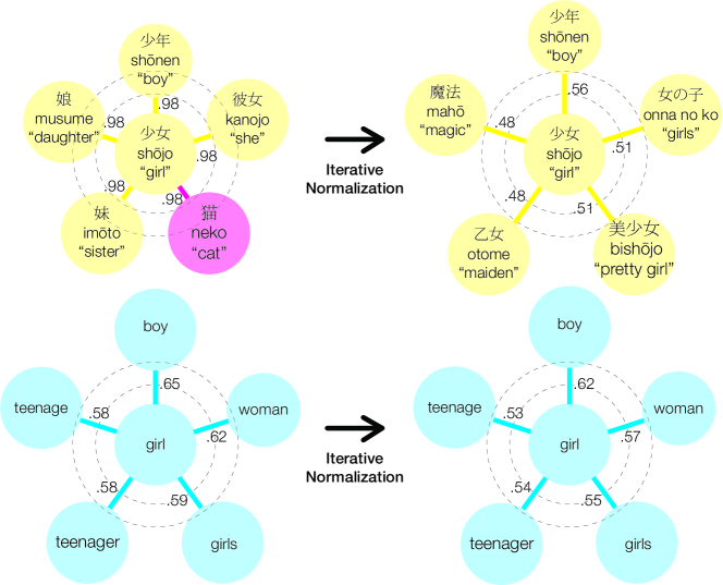
Figure 1: The most similar Japanese words for 少女 (shōjo “girl”) and English words for “girl”, measured by cosine similarity on Wikipedia fastText vectors, before (left) and after (right) Iterative Normalization. In the original embedding spaces, “boy” is the nearest neighbor for both languages but with a very different cosine similarity, and “cat” in English is not close to “girl”: both violate the isomorphism assumed by an orthogonal transformation for cross-lingual representations. Iterative Normalization replaces 猫 (neko “cat”) with the more relevant 美少女 (bishōjo “pretty girl”) and brings cosine similarities closer.

Thus, many state-of-the-art mapping-based clwe methods impose an orthogonal constraint (Artetxe et al., 2017; Conneau et al., 2018; Alvarez-Melis and Jaakkola, 2018; Artetxe et al., 2018; Ruder et al., 2018; Alvarez-Melis et al., 2019). The success of orthogonal methods relies on the assumption that embedding spaces are isomorphic; i.e., they have the same inner-product structures across languages, but this does not hold for all languages (Søgaard et al., 2018; Fujinuma et al., 2019). For example, English and Japanese fastText vectors (Bojanowski et al., 2017) have different substructures around “girl” (Figure 1 left). As a result, orthogonal mapping fails on some languages—when Hoshen and Wolf (2018) align fastText embeddings with orthogonal mappings, they report 81% English–Spanish word translation accuracy but only 2% for the more distant English–Japanese.

While recent work challenges the orthogonal assumption (Doval et al., 2018; Joulin et al., 2018; Jawanpuria et al., 2019), we focus on whether simple preprocessing techniques can improve the suitability of orthogonal models. Our iterative method normalizes monolingual embeddings to make their structures more similar (Figure 1), which improves subsequent alignment.

Our method is motivated by two desired properties of monolingual embeddings that support orthogonal alignment:

Every word vector has the same length.

Each language’s mean has the same length. Standard preprocessing such as dimension-wise mean centering and length normalization Artetxe et al. (2016) do not meet the two requirements at the same time. Our analysis leads to Iterative Normalization, an alternating projection algorithm that normalizes any word embedding to provably satisfy both conditions. After normalizing the monolingual embeddings, we then apply mapping-based clwe algorithms on the transformed embeddings.

We empirically validate our theory by combining Iterative Normalization with three mapping-based clwe methods. Iterative Normalization improves word translation accuracy on a dictionary induction benchmark across thirty-nine language pairs.

2 Learning Orthogonal Mappings

This section reviews learning orthogonal cross-lingual mapping between word embeddings and, along the way, introduces our notation.

We start with pre-trained word embeddings in a source language and a target language. We assume all embeddings are $d$-dimensional, and the two languages have the same vocabulary size $n$. Let $\bm{\mathbf{X}}\in\mathbb{R}^{d\times n}$ be the word embedding matrix for the source language, where each column $\bm{\mathbf{x}}_{i}\in\mathbb{R}^{d}$ is the representation of the $i$-th word from the source language, and let $\bm{\mathbf{Z}}\in\mathbb{R}^{d\times n}$ be the word embedding matrix for the target language. Our goal is to learn a transformation matrix $\bm{\mathbf{W}}\in\mathbb{R}^{d\times d}$ that maps the source language vectors to the target language space. While our experiments focus on the supervised case with a seed dictionary $\mathcal{D}$ with translation pairs $(i,j)$, the analysis also applies to unsupervised projection.

One straightforward way to learn $\bm{\mathbf{W}}$ is by minimizing Euclidean distances between translation pairs (Mikolov et al., 2013a). Formally, we solve:

$$\min_{\bm{\mathbf{W}}}\sum_{(i,j)\in\mathcal{D}}\|\bm{\mathbf{W}}\bm{\mathbf{x}}_{i}-\bm{\mathbf{z}}_{j}\|_{2}^{2}.$$ (1)

Xing et al. (2015) further restrict $\bm{\mathbf{W}}$ to orthogonal transformations; i.e., $\bm{\mathbf{W}}^{\top}\bm{\mathbf{W}}=\bm{\mathbf{I}}$. The orthogonal constraint significantly improves word translation accuracy (Artetxe et al., 2016). However, this method still fails for some language pairs because word embeddings are not isomorphic across languages. To improve orthogonal alignment between non-isomorphic embedding spaces, we aim to transform monolingual embeddings in a way that helps orthogonal transformation.

3 When Orthogonal Mappings Work

When are two embedding spaces easily aligned? A good orthogonal mapping is more likely if word vectors have two properties: length-invariance and center-invariance.

Length-Invariance.

First, all word vectors should have the same, constant length. Length-invariance resolves inconsistencies between monolingual word embedding and cross-lingual mapping objectives (Xing et al., 2015). During training, popular word embedding algorithms Mikolov et al. (2013b); Pennington et al. (2014); Bojanowski et al. (2017) maximize dot products between similar words, but evaluate on cosine similarity. To make things worse, the transformation matrix minimizes a third metric, Euclidean distance (Equation 1). This inconsistency is naturally resolved when the lengths of word vectors are fixed. Suppose $\bm{\mathbf{u}}\in\mathbb{R}^{d}$ and $\bm{\mathbf{v}}\in\mathbb{R}^{d}$ have the same length, then

$$\bm{\mathbf{u}}^{\top}\bm{\mathbf{v}}\propto\cos(\bm{\mathbf{u}},\bm{\mathbf{v}})=1-\frac{1}{2}\|\bm{\mathbf{u}}-\bm{\mathbf{v}}\|_{2}^{2}.$$

Minimizing Euclidean distance is equivalent to maximizing both dot product and cosine similarity with constant word vector lengths, thus making objectives consistent.

Length-invariance also satisfies a prerequisite for bilingual orthogonal alignment: the embeddings of translation pairs should have the same length. If a source word vector $\bm{\mathbf{x}}_{i}$ can be aligned to its target language translation $\bm{\mathbf{z}}_{j}=\bm{\mathbf{W}}\bm{\mathbf{x}}_{i}$ with an orthogonal matrix $\bm{\mathbf{W}}$, then

$$\|\bm{\mathbf{z}}_{j}\|_{2}=\|\bm{\mathbf{W}}\bm{\mathbf{x}}_{i}\|_{2}=\|\bm{\mathbf{x}}_{i}\|_{2},$$ (2)

where the second equality follows from the orthogonality of $\bm{\mathbf{W}}$. Equation (2) is trivially satisfied if all vectors have the same length. In summary, length-invariance not only promotes consistency between monolingual word embedding and cross-lingual mapping objective but also simplifies translation pair alignment.

Center-Invariance.

Our second condition is that the mean vector of different languages should have the same length, which we prove is a pre-requisite for orthogonal alignment. Suppose two embedding matrices $\bm{\mathbf{X}}$ and $\bm{\mathbf{Z}}$ can be aligned with an orthogonal matrix $\bm{\mathbf{W}}$ such that $\bm{\mathbf{Z}}=\bm{\mathbf{W}}\bm{\mathbf{X}}$. Let $\bm{\mathbf{\bar{x}}}=\frac{1}{n}\sum_{i=1}^{n}\bm{\mathbf{x}}_{i}$ and $\bm{\mathbf{\bar{z}}}=\frac{1}{n}\sum_{i=1}^{n}\bm{\mathbf{z}}_{i}$ be the mean vectors. Then $\bm{\mathbf{\bar{z}}}=\bm{\mathbf{W}}\bm{\mathbf{\bar{x}}}$. Since $\bm{\mathbf{W}}$ is orthogonal,

$$\|\bm{\mathbf{\bar{z}}}\|_{2}=\|\bm{\mathbf{W}}\bm{\mathbf{\bar{x}}}\|_{2}=\|\bm{\mathbf{\bar{x}}}\|_{2}.$$

In other words, orthogonal mappings can only align embedding spaces with equal-magnitude centers.

A stronger version of center-invariance is zero-mean, where the mean vector of each language is zero. Artetxe et al. (2016) find that centering improves dictionary induction; our analysis provides an explanation.

Method	Normalization	ja	zh	hi	tr	da	de	es
Procrustes	None	1.7	32.5	33.3	44.9	54.0	73.5	81.4
	c+l	12.3	41.1	34.0	46.5	54.9	74.6	81.3
	in	44.3	44.2	36.7	48.7	58.4	75.5	81.5
Procrustes + refine	None	1.7	32.5	33.6	46.3	56.8	74.3	81.9
	c+l	13.1	42.3	34.9	48.7	59.3	75.2	82.4
	in	44.3	44.2	37.7	51.7	60.9	76.0	82.5
rcsls	None	14.6	17.1	5.0	18.3	19.2	43.6	50.5
	c+l	16.1	45.1	36.2	50.7	58.3	77.5	83.6
	in	56.3	48.6	38.0	52.4	60.5	78.1	83.9

Table 1: Word translation accuracy aligning English embeddings to seven languages. We combine three normalizations—no normalization (None), mean centering and length normalization (c+l), and Iterative Normalization (in) for five rounds—with three clwes: Procrustes, Procrustes with refinement (Conneau et al., 2018), and rcsls (Joulin et al., 2018). Procrustes with c+l is equivalent to Artetxe et al. (2016). The best result for each clwe in each column in bold. Iterative Normalization has the best accuracy of the three normalization techniques.

4 Iterative Normalization

We now develop Iterative Normalization, which transforms monolingual word embeddings to satisfy both length-invariance and center-invariance. Specifically, we normalize word embeddings to simultaneously have unit-length and zero-mean. Formally, we produce embedding matrix $\bm{\mathbf{X}}$ such that

$$\|\bm{\mathbf{x}}_{i}\|_{2}=1\quad\text{for all $i$},$$ (3)

and

$$\sum_{i=1}^{n}\bm{\mathbf{x}}_{i}=\bm{\mathbf{0}}.$$ (4)

Iterative Normalization transforms the embeddings to make them satisfy both constraints at the same time. Let $\bm{\mathbf{x}}^{(0)}_{i}$ be the initial embedding for word $i$. We assume that all word embeddings are non-zero. For every word $i$, we iteratively transform each word vector $\bm{\mathbf{x}}_{i}$ by first making the vectors unit length,

$$\bm{\mathbf{y}}_{i}^{(k)}=\bm{\mathbf{x}}_{i}^{(k-1)}/\|\bm{\mathbf{x}}_{i}^{(k-1)}\|_{2},$$ (5)

and then making them mean zero,

$$\bm{\mathbf{x}}_{i}^{(k)}=\bm{\mathbf{y}}_{i}^{(k)}-\frac{1}{n}\sum_{i=1}^{n}\bm{\mathbf{y}}_{i}^{(k)}.$$ (6)

Equation (5) and (6) project the embedding matrix $\bm{\mathbf{X}}$ to the set of embeddings that satisfy Equation (3) and (4). Therefore, our method is a form of alternating projection (Bauschke and Borwein, 1996), an algorithm to find a point in the intersection of two closed sets by alternatively projecting onto one of the two sets. Alternating projection guarantees convergence in the intersection of two convex sets at a linear rate Gubin et al. (1967); Bauschke and Borwein (1993). Unfortunately, the unit-length constraint is non-convex, ruling out the classic convergence proof. Nonetheless, we use recent results on alternating non-convex projections Zhu and Li (2018) to prove Iterative Normalization’s convergence (details in Appendix A).

Theorem 1.

If the embeddings are non-zero after each iteration; i.e., $\bm{\mathbf{x}}_{i}^{(k)}\neq\bm{\mathbf{0}}$ for all $i$ and $k$, then the sequence $\left\{\bm{\mathbf{X}}^{(k)}\right\}$ produced by Iterative Normalization is convergent.

All embeddings in our experiments satisfy the non-zero assumption; it is violated only when all words have the same embedding. In degenerate cases, the algorithm might converge to a solution that does not meet the two requirements. Empirically, our method always satisfy both constraints.

Previous approach and differences.

Artetxe et al. (2016) also study he unit-length and zero-mean constraints, but our work differs in two aspects. First, they motivate the zero-mean condition based on the heuristic argument that two randomly selected word types should not be semantically similar (or dissimilar) in expectation. While this statement is attractive at first blush, some word types have more synonyms than others, so we argue that word types might not be evenly distributed in the semantic space. We instead show that zero-mean is helpful because it satisfies center-invariance, a necessary condition for orthogonal mappings. Second, Artetxe et al. (2016) attempt to enforce the two constraints by a single round of dimension-wise mean centering and length normalization. Unfortunately, this often fails to meet the constraints at the same time—length normalization can change the mean, and mean centering can change vector length. In contrast, Iterative Normalization simultaneously meets both constraints and is empirically better (Table 1) on dictionary induction.

5 Dictionary Induction Experiments

On a dictionary induction benchmark, we combine Iterative Normalization with three clwe methods and show improvement in word translation accuracy across languages.

5.1 Dataset and Methods

We train and evaluate clwe on muse dictionaries (Conneau et al., 2018) with default split. We align English embeddings to thirty-nine target language embeddings, pre-trained on Wikipedia with fastText Bojanowski et al. (2017). The alignment matrices are trained from dictionaries of 5,000 source words. We report top-1 word translation accuracy for 1,500 source words, using cross-domain similarity local scaling (Conneau et al., 2018, csls). We experiment with the following clwe methods.

Procrustes Analysis.

Our first algorithm uses Procrustes analysis Schönemann (1966) to find the orthogonal transformation that minimizes Equation 1, the total distance between translation pairs.

Post-hoc Refinement.

Orthogonal mappings can be improved with refinement steps Artetxe et al. (2017); Conneau et al. (2018). After learning an initial mapping $\bm{\mathbf{W}}_{0}$ from the seed dictionary $\mathcal{D}$, we build a synthetic dictionary $\mathcal{D}_{1}$ by translating each word with $\bm{\mathbf{W}}_{0}$. We then use the new dictionary $\mathcal{D}_{1}$ to learn a new mapping $\bm{\mathbf{W}}_{1}$ and repeat the process.

Relaxed csls Loss (rcsls).

Joulin et al. (2018) optimize csls scores between translation pairs instead of Equation (1). rcsls has state-of-the-art supervised word translation accuracies on muse (Glavas et al., 2019). For the ease of optimization, rcsls does not enforce the orthogonal constraint. Nevertheless, Iterative Normalization also improves its accuracy (Table 1), showing it can help linear non-orthogonal mappings too.

5.2 Training Details

We use the implementation from muse for Procrustes analysis and refinement (Conneau et al., 2018). We use five refinement steps. For rcsls, we use the same hyperparameter selection strategy as Joulin et al. (2018)—we choose learning rate from $\{1,10,25,50\}$ and number of epochs from $\{10,20\}$ by validation. As recommended by Joulin et al. (2018), we turn off the spectral constraint. We use ten nearest neighbors when computing csls.

5.3 Translation Accuracy

For each method, we compare three normalization strategies: (1) no normalization, (2) dimension-wise mean centering followed by length normalization (Artetxe et al., 2016), and (3) five rounds of Iterative Normalization. Table 1 shows word translation accuracies on seven selected target languages. Results on other languages are in Appendix B.

As our theory predicts, Iterative Normalization increases translation accuracy for Procrustes analysis (with and without refinement) across languages. While centering and length-normalization also helps, the improvement is smaller, confirming that one round of normalization is insufficient. The largest margin is on English-Japanese, where Iterative Normalization increases test accuracy by more than 40%. Figure 1 shows an example of how Iterative Normalization makes the substructure of an English-Japanese translation pair more similar.

Surprisingly, normalization is even more important for rcsls, a clwe method without orthogonal constraint. rcsls combined with Iterative Normalization has state-of-the-art accuracy, but rcsls is much worse than Procrustes analysis on unnormalized embeddings, suggesting that length-invariance and center-invariance are also helpful for learning linear non-orthogonal mappings.

Dataset	Before	After
ws-353	73.9	73.7
mc	81.2	83.9
rg	79.7	80.0
yp-130	53.3	57.6

Table 2: Correlations before and after applying Iterative Normalization on four English word similarity benchmarks: ws-353 (Finkelstein et al., 2002), mc (Miller and Charles, 1991), rg (Rubenstein and Goodenough, 1965), and yp-130 (Yang and Powers, 2006). The scores are similar, which shows that Iterative Normalization retains useful structures from the original embeddings.

5.4 Monolingual Word Similarity

Many trivial solutions satisfy both length-invariance and center-invariance; e.g., we can map half of words to $\bm{\mathbf{e}}$ and the rest to $-\bm{\mathbf{e}}$, where $\bm{\mathbf{e}}$ is any unit-length vector. A meaningful transformation should also preserve useful structure in the original embeddings. We confirm Iterative Normalization does not hurt scores on English word similarity benchmarks (Table 2), showing that Iterative Normalization produces meaningful representations.

6 Conclusion

We identify two conditions that make cross-lingual orthogonal mapping easier: length-invariance and center-invariance, and provide a simple algorithm that transforms monolingual embeddings to satisfy both conditions. Our method improves word translation accuracy of different mapping-based clwe algorithms across languages. In the future, we will investigate whether our method helps other downstream tasks.

Appendix A Proof for Theorem 1

Our convergence analysis is based on a recent result on alternating non-convex projections. Theorem 1 in the work of  Zhu and Li (2018) states that the convergence of alternating projection holds even if the constraint sets are non-convex, as long as the two constraint sets satisfy the following assumption:

Assumption 1.

Let $\mathbb{X}$ and $\mathbb{Y}$ be any two closed semi-algebraic sets, and let $\left\{\left(\bm{\mathbf{x}}_{k},\bm{\mathbf{y}}_{k}\right)\right\}$ be the sequence of iterates generated by the alternating projection method (e.g., Iterative Normalization). Assume the sequence $\left\{\left(\bm{\mathbf{x}}_{k},\bm{\mathbf{y}}_{k}\right)\right\}$ is bounded and the sets $\mathbb{X}$ and $\mathbb{Y}$ obey the following properties:

1. three-point property of $\mathbb{Y}$: there exists a nonnegative function $\delta_{\alpha}:\mathbb{Y}\times\mathbb{Y}\rightarrow\mathbb{R}$ with $\alpha>0$ such that for any $k\geq 1$, we have

   $$\delta_{\alpha}\left(\bm{\mathbf{y}}_{k},\bm{\mathbf{y}}_{k-1}\right)\geq\alpha\|\bm{\mathbf{y}}_{k}-\bm{\mathbf{y}}_{k-1}\|_{2}$$

   and

   $$\delta_{\alpha}\left(\bm{\mathbf{y}}_{k-1},\bm{\mathbf{y}}_{k}\right)+\|\bm{\mathbf{x}}_{k}-\bm{\mathbf{y}}_{k}\|_{2}^{2}\\ \leq\|\bm{\mathbf{x}}_{k}-\bm{\mathbf{y}}_{k-1}\|_{2}^{2},$$

2. local contraction property of $\mathbb{X}$: there exist $\epsilon>0$ and $\beta>0$ such that when $\|\bm{\mathbf{y}}_{k}-\bm{\mathbf{y}}_{k-1}\|_{2}\leq\epsilon$, we have

   $$\|\bm{\mathbf{x}}_{k+1}-\bm{\mathbf{x}}_{k}\|_{2} =\|\mathcal{P}_{\mathbb{X}}(\bm{\mathbf{y}}_{k})-\mathcal{P}_{\mathbb{X}}(\bm{\mathbf{y}}_{k-1})\|_{2}$$

   $$\leq\beta\|\bm{\mathbf{y}}_{k}-\bm{\mathbf{y}}_{k-1}\|_{2}$$

   where $\mathcal{P}_{\mathbb{X}}$ is the projection onto ${\mathbb{X}}$.

Zhu and Li (2018) only consider sets of vectors, but our constraint are sets of matrices. For ease of exposition, we treat every embedding matrix $\bm{\mathbf{X}}\in\mathbb{R}^{d\times n}$ as a vector by concatenating the column vectors: $\bm{\mathbf{X}}=[\bm{\mathbf{x}}_{1},\bm{\mathbf{x}}_{2},\cdots,\bm{\mathbf{x}}_{n}]$. The $l^{2}$-norm of the concatenated vector $\|\bm{\mathbf{X}}\|_{2}$ is equivalent to the Frobenius norm of the original matrix $\|\bm{\mathbf{X}}\|_{F}$.

The two operations in Iterative Normalization, Equation (5) and (6), are projections onto two constraint sets, unit-length set $\mathbb{Y}=\left\{\bm{\mathbf{X}}\in\mathbb{R}^{d\times n}:\forall i,\|\bm{\mathbf{x}}_{i}\|_{2}=1\right\}$ and zero-mean set $\mathbb{X}=\left\{\bm{\mathbf{X}}\in\mathbb{R}^{d\times n}:\sum_{i=1}^{n}\bm{\mathbf{x}}_{i}=\bm{\mathbf{0}}\right\}$. To prove convergence of Iterative Normalization, we show that $\mathbb{Y}$ satisfies the three-point property, and $\mathbb{X}$ satisfies the local contraction property.

Three-point property of $\mathbb{Y}$.

For any $\bm{\mathbf{Y}}^{\prime}\in\mathbb{Y}$ and $\bm{\mathbf{X}}\in\mathbb{R}^{n\times d}$, let $\bm{\mathbf{Y}}$ be the projection of $\bm{\mathbf{X}}$ onto the constraint set $\mathbb{Y}$ with Equation (5). The columns of $\bm{\mathbf{Y}}$ and $\bm{\mathbf{Y^{\prime}}}$ have the same length, so we have

$$\|\bm{\mathbf{X}}-\bm{\mathbf{Y}}^{\prime}\|_{2}^{2}-\|\bm{\mathbf{X}}-\bm{\mathbf{Y}}\|_{2}^{2}$$

$$\quad=\sum_{i=1}^{n}\|\bm{\mathbf{x}}_{i}-\bm{\mathbf{y}}^{\prime}_{i}\|^{2}-\|\bm{\mathbf{x}}_{i}-\bm{\mathbf{y}}_{i}\|_{2}^{2}$$

$$\quad=\sum_{i=1}^{n}2\bm{\mathbf{x}}_{i}^{\top}\bm{\mathbf{y}}_{i}-2\bm{\mathbf{x}}_{i}^{\top}\bm{\mathbf{y}}^{\prime}_{i}.$$ (7)

Since $\bm{\mathbf{Y}}$ is the projection of $\bm{\mathbf{X}}$ onto the unit-length set with Equation (5); i.e., $\bm{\mathbf{y}}_{i}=\bm{\mathbf{x}}_{i}/\|\bm{\mathbf{x}}_{i}\|_{2}$, we can rewrite Equation (7).

$$\|\bm{\mathbf{X}}-\bm{\mathbf{Y}}^{\prime}\|_{2}^{2}-\|\bm{\mathbf{X}}-\bm{\mathbf{Y}}\|_{2}^{2}$$

$$\quad=\sum_{i=1}^{n}\|\bm{\mathbf{x}}_{i}\|_{2}(2\bm{\mathbf{y}}_{i}^{\top}\bm{\mathbf{y}}_{i}-2\bm{\mathbf{y}}_{i}^{\top}\bm{\mathbf{y}}^{\prime}_{i}).$$ (8)

All columns of $\bm{\mathbf{Y}}$ and $\bm{\mathbf{Y^{\prime}}}$ are unit-length. Therefore, we can further rewrite Equation (8).

$$\|\bm{\mathbf{X}}-\bm{\mathbf{Y}}^{\prime}\|_{2}^{2}-\|\bm{\mathbf{X}}-\bm{\mathbf{Y}}\|_{2}^{2}$$

$$\quad=\sum_{i=1}^{n}\|\bm{\mathbf{x}}_{i}\|_{2}(2-2\bm{\mathbf{y}}_{i}^{\top}\bm{\mathbf{y}}^{\prime}_{i})$$

$$\quad=\sum_{i=1}^{n}\|\bm{\mathbf{x}}_{i}\|_{2}\|\bm{\mathbf{y}}_{i}-\bm{\mathbf{y}}^{\prime}_{i}\|_{2}^{2}.$$

Let $l=\min_{i}\left\{\|\bm{\mathbf{x}}_{i}\|_{2}\right\}$ be the minimum length of the columns in $\bm{\mathbf{X}}$. We have the following inequality:

$$\|\bm{\mathbf{X}}-\bm{\mathbf{Y}}^{\prime}\|_{2}^{2}-\|\bm{\mathbf{X}}-\bm{\mathbf{Y}}\|_{2}^{2}$$

$$\quad\geq\sum_{i=1}^{n}l\|\bm{\mathbf{y}}_{i}-\bm{\mathbf{y}}^{\prime}_{i}\|_{2}^{2}$$

$$\quad=l||\bm{\mathbf{Y}}-\bm{\mathbf{Y}}^{\prime}\|_{2}^{2}.$$

From our non-zero assumption, the minimum column length $l$ is always positive. Let $l_{k}$ be the minimum column length of the embedding matrix $\bm{\mathbf{X}}^{(k)}$ after the $k$-th iteration. It follows that $\mathbb{Y}$ satisfies the three-point property with $\alpha=\min_{k}\left\{l_{k}\right\}$ and $\delta_{\alpha}(\bm{\mathbf{Y}},\bm{\mathbf{Y}}^{\prime})=\alpha\|\bm{\mathbf{Y}}-\bm{\mathbf{Y}}^{\prime}\|_{2}^{2}$.

Local contraction property of $\mathbb{X}$.

The zero-mean constraint set $\mathbb{X}$ is convex and closed: if two matrices $\bm{\mathbf{X}}$ and $\bm{\mathbf{Y}}$ both have zero-mean, their linear interpolation $\lambda\bm{\mathbf{X}}+(1-\lambda)\bm{\mathbf{Y}}$ must also have zero-mean for any $0<\lambda<1$. Projections onto convex sets in a Hilbert space are contractive Browder (1967), and therefore $\mathbb{X}$ satisfies the local contraction property with any positive $\epsilon$ and $\beta=1$.

In summary, the two constraint sets that Iterative Normalization projects onto satisfy Assumption 1. Therefore, Iterative Normalization converges following the analysis of Zhu and Li (2018).

Appendix B Results on All Languages

Table 3 shows word translation accuracies on all target languages. Iterative Normalization improves accuracy on all languages.

	Procrustes			Procrustes + refine			rcsls
Target	None	c+l	in	None	c+l	in	None	c+l	in
af	26.3	28.3	29.7	27.7	28.7	30.4	9.3	28.6	29.3
ar	36.5	37.1	37.9	36.5	37.1	37.9	18.4	40.5	41.5
bs	22.3	23.5	24.4	23.3	23.9	26.6	5.4	25.5	26.6
ca	65.9	67.6	68.9	66.5	67.6	68.9	43.0	68.9	69.5
cs	54.0	54.7	55.3	54.0	54.7	55.7	29.9	57.8	58.2
da	54.0	54.9	58.4	56.8	59.3	60.9	19.2	58.3	60.5
de	73.5	74.6	75.5	74.3	75.2	76.0	43.6	77.5	78.1
el	44.0	44.9	47.5	44.6	45.9	47.9	14.0	47.1	48.5
es	81.4	81.3	81.5	81.9	82.1	82.5	50.5	83.6	83.9
et	31.9	34.5	36.1	31.9	35.3	36.4	8.1	37.3	39.4
fa	33.1	33.7	37.3	33.1	34.1	37.3	5.9	37.5	38.3
fi	47.6	48.5	50.9	47.6	50.1	51.1	20.9	52.3	53.3
fr	81.1	81.3	81.7	82.1	82.7	82.4	53.1	83.9	83.9
he	40.2	43.1	43.7	40.2	43.1	43.7	13.1	49.7	50.1
hi	33.3	34.0	36.7	33.6	34.9	37.7	5.0	36.2	38.0
hr	37.0	37.8	40.2	37.6	37.8	40.2	14.5	41.1	42.6
hu	51.8	54.1	55.5	53.3	54.1	56.1	11.7	57.3	58.2
id	65.6	65.7	67.9	67.7	68.4	70.3	24.8	68.9	70.0
it	76.2	76.6	76.6	77.5	78.1	78.1	48.4	78.8	79.1
ja	1.7	13.1	44.3	1.7	13.1	44.3	14.6	16.1	56.3
ko	31.5	32.1	33.9	31.5	32.1	33.9	6.4	37.5	37.5
lt	22.5	22.8	23.2	22.5	22.8	23.3	7.6	23.3	23.5
lv	23.6	24.9	26.1	23.6	24.9	26.1	10.1	28.3	28.7
ms	44.0	45.4	48.9	46.5	48.3	51.1	19.9	49.1	50.2
nl	72.8	73.7	74.1	73.8	75.1	75.8	46.7	75.6	75.8
pl	58.2	60.2	60.1	58.5	60.2	60.4	39.4	62.4	62.5
pt	79.5	79.7	79.9	79.9	81.0	81.2	63.1	81.1	81.7
ro	58.1	60.5	61.8	59.9	60.5	62.5	27.1	61.9	63.3
ru	51.7	52.1	52.1	51.7	52.1	52.1	26.6	57.1	57.9
sk	38.0	39.3	40.4	38.0	39.3	41.7	13.3	41.5	42.3
sl	32.5	34.3	36.7	32.5	34.4	36.7	12.3	36.0	37.9
sq	23.5	25.1	27.3	23.5	25.1	27.3	4.4	26.5	27.3
sv	58.7	59.6	60.7	60.9	61.2	62.6	35.6	63.8	63.9
ta	15.1	15.5	16.8	15.1	15.5	17.7	6.7	16.3	17.1
th	22.5	23.3	22.9	22.5	23.3	22.9	9.4	23.7	23.9
tr	44.9	46.5	48.7	46.3	48.7	51.7	18.3	50.7	52.4
uk	34.8	35.9	36.3	35.5	35.9	36.5	18.8	40.7	40.8
vi	41.3	42.1	43.7	42.1	42.7	44.2	14.2	43.3	43.9
zh	32.5	42.3	44.2	32.5	42.3	44.2	17.1	45.1	48.6
Average	44.7	46.3	48.4	45.3	47.0	49.1	21.8	49.0	50.9

Table 3: Word translation accuracy aligning English embeddings to thirty-nine languages. We combine three normalizations—no normalization (None), mean centering and length normalization (c+l), and Iterative Normalization (in) for five rounds—with three clwes: Procrustes, Procrustes with refinement (Conneau et al., 2018), and rcsls (Joulin et al., 2018). Procrustes with c+l is equivalent to Artetxe et al. (2016). The best result for each clwe in each column in bold. Iterative Normalization has the best accuracy of the three normalization techniques.

References

- Alvarez-Melis and Jaakkola (2018) David Alvarez-Melis and Tommi S. Jaakkola. 2018. Gromov-wasserstein alignment of word embedding spaces. In Proceedings of Empirical Methods in Natural Language Processing.
- Alvarez-Melis et al. (2019) David Alvarez-Melis, Stefanie Jegelka, and Tommi S Jaakkola. 2019. Towards optimal transport with global invariances. In Proceedings of Artificial Intelligence and Statistics.
- Artetxe et al. (2016) Mikel Artetxe, Gorka Labaka, and Eneko Agirre. 2016. Learning principled bilingual mappings of word embeddings while preserving monolingual invariance. In Proceedings of Empirical Methods in Natural Language Processing.
- Artetxe et al. (2017) Mikel Artetxe, Gorka Labaka, and Eneko Agirre. 2017. Learning bilingual word embeddings with (almost) no bilingual data. In Proceedings of the Association for Computational Linguistics.
- Artetxe et al. (2018) Mikel Artetxe, Gorka Labaka, and Eneko Agirre. 2018. A robust self-learning method for fully unsupervised cross-lingual mappings of word embeddings. In Proceedings of the Association for Computational Linguistics.
- Bauschke and Borwein (1993) Heinz H. Bauschke and Jonathan M. Borwein. 1993. On the convergence of von Neumann’s alternating projection algorithm for two sets. Set-Valued Analysis, 1(2):185–212.
- Bauschke and Borwein (1996) Heinz H. Bauschke and Jonathan M. Borwein. 1996. On projection algorithms for solving convex feasibility problems. SIAM review, 38(3):367–426.
- Bojanowski et al. (2017) Piotr Bojanowski, Edouard Grave, Armand Joulin, and Tomas Mikolov. 2017. Enriching word vectors with subword information. Transactions of the Association for Computational Linguistics, 5:135–146.
- Browder (1967) Felix E. Browder. 1967. Convergence of approximants to fixed points of nonexpansive nonlinear mappings in Banach spaces. Archive for Rational Mechanics and Analysis, 24(1):82–90.
- Conneau et al. (2018) Alexis Conneau, Guillaume Lample, Marc’Aurelio Ranzato, Ludovic Denoyer, and Hervé Jégou. 2018. Word translation without parallel data. In Proceedings of the International Conference on Learning Representations.
- Doval et al. (2018) Yerai Doval, Jose Camacho-Collados, Luis Espinosa-Anke, and Steven Schockaert. 2018. Improving cross-lingual word embeddings by meeting in the middle. In Proceedings of Empirical Methods in Natural Language Processing.
- Finkelstein et al. (2002) Lev Finkelstein, Evgeniy Gabrilovich, Yossi Matias, Ehud Rivlin, Zach Solan, Gadi Wolfman, and Eytan Ruppin. 2002. Placing search in context: The concept revisited. ACM Transactions on information systems, 20(1):116–131.
- Fujinuma et al. (2019) Yoshinari Fujinuma, Jordan Boyd-Graber, and Michael J. Paul. 2019. A resource-free evaluation metric for cross-lingual word embeddings based on graph modularity. In Proceedings of the Association for Computational Linguistics.
- Glavas et al. (2019) Goran Glavas, Robert Litschko, Sebastian Ruder, and Ivan Vulic. 2019. How to (properly) evaluate cross-lingual word embeddings: On strong baselines, comparative analyses, and some misconceptions. In Proceedings of the Association for Computational Linguistics.
- Gubin et al. (1967) L.G. Gubin, B.T. Polyak, and E.V. Raik. 1967. The method of projections for finding the common point of convex sets. USSR Computational Mathematics and Mathematical Physics, 7(6):1–24.
- Guo et al. (2015) Jiang Guo, Wanxiang Che, David Yarowsky, Haifeng Wang, and Ting Liu. 2015. Cross-lingual dependency parsing based on distributed representations. In Proceedings of the Association for Computational Linguistics.
- Hoshen and Wolf (2018) Yedid Hoshen and Lior Wolf. 2018. Non-adversarial unsupervised word translation. In Proceedings of Empirical Methods in Natural Language Processing.
- Jawanpuria et al. (2019) Pratik Jawanpuria, Arjun Balgovind, Anoop Kunchukuttan, and Bamdev Mishra. 2019. Learning multilingual word embeddings in latent metric space: a geometric approach. Transactions of the Association for Computational Linguistics, 7:107–120.
- Joulin et al. (2018) Armand Joulin, Piotr Bojanowski, Tomas Mikolov, Hervé Jégou, and Edouard Grave. 2018. Loss in translation: Learning bilingual word mapping with a retrieval criterion. In Proceedings of Empirical Methods in Natural Language Processing.
- Klementiev et al. (2012) Alexandre Klementiev, Ivan Titov, and Binod Bhattarai. 2012. Inducing crosslingual distributed representations of words. Proceedings of International Conference on Computational Linguistics.
- Mikolov et al. (2013a) Tomas Mikolov, Quoc V. Le, and Ilya Sutskever. 2013a. Exploiting similarities among languages for machine translation. arXiv preprint arXiv:1309.4168.
- Mikolov et al. (2013b) Tomas Mikolov, Ilya Sutskever, Kai Chen, Gregory S. Corrado, and Jeffrey Dean. 2013b. Distributed representations of words and phrases and their compositionality. In Proceedings of Advances in Neural Information Processing Systems.
- Miller and Charles (1991) George A. Miller and Walter G. Charles. 1991. Contextual correlates of semantic similarity. Language and Cognitive Processes, 6(1):1–28.
- Pennington et al. (2014) Jeffrey Pennington, Richard Socher, and Christopher D. Manning. 2014. GloVe: Global vectors for word representation. In Proceedings of Empirical Methods in Natural Language Processing.
- Rubenstein and Goodenough (1965) Herbert Rubenstein and John B Goodenough. 1965. Contextual correlates of synonymy. Communications of the ACM, 8(10):627–633.
- Ruder et al. (2018) Sebastian Ruder, Ryan Cotterell, Yova Kementchedjhieva, and Anders Søgaard. 2018. A discriminative latent-variable model for bilingual lexicon induction. In Proceedings of Empirical Methods in Natural Language Processing.
- Ruder et al. (2017) Sebastian Ruder, Ivan Vulić, and Anders Søgaard. 2017. A survey of cross-lingual embedding models. arXiv preprint arXiv:1706.04902.
- Schönemann (1966) Peter H. Schönemann. 1966. A generalized solution of the orthogonal procrustes problem. Psychometrika, 31(1):1–10.
- Smith et al. (2017) Samuel L. Smith, David H. P. Turban, Steven Hamblin, and Nils Y. Hammerla. 2017. Offline bilingual word vectors, orthogonal transformations and the inverted softmax. In Proceedings of the International Conference on Learning Representations.
- Søgaard et al. (2018) Anders Søgaard, Sebastian Ruder, and Ivan Vulić. 2018. On the limitations of unsupervised bilingual dictionary induction. In Proceedings of the Association for Computational Linguistics.
- Xing et al. (2015) Chao Xing, Dong Wang, Chao Liu, and Yiye Lin. 2015. Normalized word embedding and orthogonal transform for bilingual word translation. In Conference of the North American Chapter of the Association for Computational Linguistics.
- Yang and Powers (2006) Dongqiang Yang and David M. Powers. 2006. Verb similarity on the taxonomy of wordnet. In International WordNet Conference.
- Zhang et al. (2016) Yuan Zhang, David Gaddy, Regina Barzilay, and Tommi Jaakkola. 2016. Ten pairs to tag – multilingual POS tagging via coarse mapping between embeddings. In Conference of the North American Chapter of the Association for Computational Linguistics.
- Zhu and Li (2018) Zhihui Zhu and Xiao Li. 2018. Convergence analysis of alternating nonconvex projections. arXiv preprint arXiv:1802.03889.