Covariate-Powered Empirical Bayes Estimation

Abstract

We study methods for simultaneous analysis of many noisy experiments in the presence of rich covariate information. The goal of the analyst is to optimally estimate the true effect underlying each experiment. Both the noisy experimental results and the auxiliary covariates are useful for this purpose, but neither data source on its own captures all the information available to the analyst. In this paper, we propose a flexible plug-in empirical Bayes estimator that synthesizes both sources of information and may leverage any black-box predictive model. We show that our approach is within a constant factor of minimax for a simple data-generating model. Furthermore, we establish robust convergence guarantees for our method that hold under considerable generality, and exhibit promising empirical performance on both real and simulated data.

1 Introduction

It is nowadays common for a geneticist to simultaneously study the association of thousands of different genes with a disease (Efron et al., 2001; Lönnstedt and Speed, 2002; Love et al., 2014), for a technology firm to have records from thousands of randomized experiments (McMahan et al., 2013), or for a social scientist to examine data from hundreds of different regions at once (Abadie and Kasy, 2018). In all of these settings, we are fundamentally interested in learning something about each sample (i.e., gene, experimental intervention, etc.) on its own; however, the abundance of data on other samples can give us useful context with which to interpret our measurements about each individual sample (Efron, 2010; Robbins, 1964). In this paper, we propose a method for simultaneous analysis of many noisy experiments, and show that it is able to exploit rich covariate information for improved power by leveraging existing machine learning tools geared towards a basic prediction task.

As a motivation for our statistical setting, suppose we have access to a dataset of movie reviews where each movie $i=1,\,...,\,n$ has an average rating $Z_{i}$ over a limited number of viewers; we also have access to a number of covariates $X_{i}$ about the movie (e.g., genre, length, cast, etc.). The task is to estimate the “true” rating $\mu_{i}$ of the movie, i.e., the average rating had the movie been reviewed by a large number of reviewers similar to the ones who already reviewed it. A first simple approach to estimating $\mu_{i}$ is to use its observed average rating as a point estimate, i.e., to set $\hat{\mu}_{i}=Z_{i}$. This approach is clearly valid for movies where we have enough data for sampling noise to dissipate, e.g., with over 50,000 reviews in the MovieLens 20M data (Harper and Konstan, 2016), we expect the 4.2/5 rating of Pulp Fiction to be quite stable. Conversely, for movies with fewer reviews, this strategy may be unstable: the rating 1.6/5 of Urban Justice is based on less than 20 reviews, and appears liable to change as we collect more data. A second alternative would be to just rely on covariates: We could learn to predict average ratings from covariates, $m(x)=\mathbb{E}\left[Z_{i}\,\big{|}\,X_{i}=x\right]$, and then set $\hat{\mu}_{i}=\hat{m}(X_{i})$. This may be more appropriate than using the observed mean rating for movies with very few reviews, but is limited in its accuracy if the covariates aren’t expressive enough to perfectly capture $\mu_{i}$.

We develop an approach that reconciles (and optimally interpolates between) the two estimation strategies discussed above. The starting point for our discussion is the following generative model,

$$X_{i}\sim\mathbb{P}^{X},\;\;\mu_{i}\mid X_{i}\sim\mathcal{N}\left(m(X_{i}),\,A\right),\;\;Z_{i}\mid\mu_{i}\sim\mathcal{N}\left(\mu_{i},\,\sigma^{2}\right),$$ (1)

according to which the true rating $\mu_{i}$ of each movie is partially explained by its covariates $X_{i}$, but also has an idiosyncratic and unpredictable component with a Gaussian distribution $\mathcal{N}\left(0,\,A\right)$. Recall that we observe $X_{i}$ and $Z_{i}$ for each $i=1,\,...,\,n$, and want to estimate the vector of $\mu_{i}$. Given this setting, if we knew both the idiosyncratic noise level $A$ and $m(x)$, the conditional mean of $\mu_{i}$ given $X_{i}=x$, then the mean-square-error-optimal estimate of $\mu_{i}$ could directly be read off of Bayes’ rule, $\hat{\mu}_{i}^{*}=t^{*}_{m,A}(X_{i},\,Z_{i})$, with

$$t^{*}_{m,A}(x,z):=\mathbb{E}_{m,A}\left[\mu_{i}\mid X_{i}=x,\,Z_{i}=z\right]=\frac{A}{\sigma^{2}+A}z+\frac{\sigma^{2}}{\sigma^{2}+A}m(x).$$ (2)

As shown in Figure 1, the behavior of this shrinker depends largely on the ratio $A/\sigma^{2}$: As this ratio gets large, the Bayes rule gets close to just setting $\hat{\mu}_{i}=Z_{i}$, whereas when the ratio is small, it shrinks everything to predictions made using covariates.

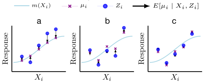
Figure 1: Optimal empirical Bayes shrinkage. All three plots show $\mu_{i}$ and $Z_{i}$ drawn from (1) for various values of $A/\sigma^{2}$, with the covariate values $X_{i}$ fixed and the regression curve $m(\cdot)$ shown in blue. The arrows depict how the oracle Bayes denoiser from (2) moves the point estimate $\hat{\mu}_{i}$ away from the raw observation $Z_{i}$ and towards $m(X_{i})$. a) When $A/\sigma^{2}=0$, the oracle estimator shrinks $Z_{i}$ all the way back to $m(X_{i})$. b) For $A/\sigma^{2}=1$, optimal shrinkage uses $(Z_{i}+m(X_{i}))/2$ to estimate $\mu_{i}$. c) When $A/\sigma^{2}$ is very large, it is preferable to discard $m(X_{i})$ and just use the information in $Z_{i}$.

Now in practice, $m(\cdot)$ and $A$ are unlikely to be known a-priori and, furthermore, we may not believe that the hierarchical structure (1) is a perfect description of the underlying data-generating process. The main contribution of this paper is an estimation strategy that addresses these challenges. First, we derive the minimax risk for estimating $\mu_{i}$ in model (1) in a setting where $m(\cdot)$ is unknown but we are willing to make various regularity assumptions (e.g., that $m(\cdot)$ is Lipschitz). Second, we show that a feasible plug-in version of (2) with estimated $\hat{m}(\cdot)$ and $\widehat{A}$ attains this lower bound up to constants that do not depend on $\sigma^{2}$ or $A$.

Finally, we consider robustness of our approach to misspecification of the model (1), and establish an extension to the classic result of James and Stein (1961), whereby without any assumptions on the distribution of $\mu_{i}$ conditionally on $X_{i}$, we can show that our approach still improves over both simple baselines $\hat{\mu}_{i}=Z_{i}$ and $\hat{\mu}_{i}=\hat{m}(X_{i})$ in considerable generality (see Section 4 for precise statements). We also consider behavior of our estimator in situations where the distribution of $Z_{i}$ conditionally on $\mu_{i},X_{i}$ may not be Gaussian, and the conditional variance $\sigma^{2}_{i}$ of $Z_{i}$ given $\mu_{i},X_{i}$ may be different for different samples.

Our approach builds on a long tradition of empirical Bayes estimation that seeks to establish frequentist guarantees for plug-in Bayesian estimators and related procedures in data-rich environments (Efron, 2010; Robbins, 1964). Empirical Bayes estimation in the setting without covariates $X_{i}$ is by now well understood (Brown and Greenshtein, 2009; Efron, 2011; Efron and Morris, 1973; Ignatiadis et al., 2019; Ignatiadis and Wager, 2019; James and Stein, 1961; Jiang and Zhang, 2009; Johnstone and Silverman, 2004; Muralidharan, 2010; Stephens, 2016; Weinstein et al., 2018).

In contrast, empirical Bayes analysis with covariates has been less comprehensively explored, and existing formal results are confined to special cases. Fay and Herriot (1979) introduced a model of the form (1) with a linear specification, $m(x)=x^{\top}\beta$, motivated by the problem of “small area estimation” that arises when studying small groups of people based on census data. Further properties of empirical Bayes estimators in the linear specification (including robustness to misspecification) were established by Green and Strawderman (1991) in the case where $X_{i}\in\mathbb{R}$ and $m(x)=x$, and by Cohen et al. (2013); Tan (2016) and Kou and Yang (2017) when $m(x)=x^{\top}\beta$. There has also been some work on empirical Bayes estimation with nonparametric specifications for $m$, e.g., Mukhopadhyay and Maiti (2004) and Opsomer et al. (2008). In a genetics application, Stephan et al. (2015) parametrized $m(x)$ as a random forest. Banerjee et al. (2018) utilize univariate side information to estimate sequences of $\mu_{i}$ that consist mostly of zeros. We also note recent work by Coey and Cunningham (2019) who considered experiment splitting as an alternative to empirical Bayes estimation. Our paper adds to this body of knowledge by providing the first characterization of minimax-optimal error in the general model (1), by proposing a flexible estimator that attains this bound up to constants, and by studying robustness of non-parametric empirical Bayes methods to model misspecification.

2 Minimax rates for empirical Bayes estimation with covariates

We first develop minimax optimality theory for model (1), when $m$ is known to lie in a class $\mathcal{C}$ of functions. To this end, we formalize the notion of regret in empirical Bayes estimation, following Robbins (1964). Concretely, as before, we assume that we have access to $n$ i.i.d. copies $(X_{i},Z_{i})$ from model (1); $\mu_{i}$ is not observed. Our task at hand then is to construct a denoiser $\hat{t}_{n}:\mathcal{X}\times\mathbb{R}\to\mathbb{R}$ that we will use to estimate $\mu_{n+1}$ by $\hat{t}_{n}(X_{n+1},Z_{n+1})$ for a future sample $(X_{n+1},\,Z_{n+1})$. We benchmark this estimator against the unknown Bayes estimator $t^{*}_{m,A}(X_{n+1},Z_{n+1})$ from  (2) in terms of its regret (excess risk) $L(\hat{t}_{n};m,A)$, where:

$$L(t;m,A):=\mathbb{E}_{m,A}\left[\left(t(X_{n+1},Z_{n+1})-\mu_{n+1}\right)^{2}\right]-\mathbb{E}_{m,A}\left[\left(t_{m,A}^{*}(X_{n+1},Z_{n+1})-\mu_{n+1}\right)^{2}\right]$$ (3)

We characterize the difficulty of this task by exhibiting the minimax rates for the empirical Bayes excess risk incurred by not knowing $m\in\mathcal{C}$ (but knowing $A$), where $\mathcal{C}$ is a pre-specified class of functions:

$$\mathfrak{M}_{n}^{\text{EB}}\left(\mathcal{C};A,\sigma^{2}\right):=\inf_{\hat{t}_{n}}\sup_{m\in\mathcal{C}}\left\{\mathbb{E}_{m,A}\left[L(\hat{t}_{n};m,A)\right]\right\}$$ (4)

Our key result, informally stated, is that the minimax excess risk $\mathfrak{M}_{n}^{\text{EB}}$ can be characterized in terms of the minimax risk for estimating $m(\cdot)$ with respect to $L^{2}(\mathbb{P}^{X})$ in the regression problem in which we observe $\smash{(X_{i},Z_{i})_{1\leq i\leq n}}$ with $\smash{Z_{i}\mid X_{i}\sim\mathcal{N}(m(X_{i}),\,A+\sigma^{2})}$, i.e.,

$$\mathfrak{M}_{n}^{\text{Reg}}\left(\mathcal{C};A+\sigma^{2}\right):=\inf_{\hat{m}_{n}}\sup_{m\in\mathcal{C}}\mathbb{E}_{m,A}\left[\int\left(\hat{m}_{n}(x)-m(x)\right)^{2}d\mathbb{P}^{X}(x)\right],$$ (5)

such that, for many commonly used function classes $\mathcal{C}$, we have

$$\mathfrak{M}_{n}^{\text{EB}}\left(\mathcal{C};A,\sigma^{2}\right)\asymp\frac{\sigma^{4}}{\left(\sigma^{2}+A\right)^{2}}\mathfrak{M}_{n}^{\text{Reg}}\left(\mathcal{C};A+\sigma^{2}\right).$$ (6)

In other words, when $A/\sigma^{2}$ is very large, we find that it is easy to match the performance of Bayes rule (2), since it collapses to $Z_{i}$. On the other hand, when $A/\sigma^{2}$ is small, matching the Bayes rule requires estimating $m(\cdot)$ well, and (6) precisely describes how the difficulty of estimating $m(\cdot)$ affects our problem of interest.

Previous work on minimax rates for the excess risk (3) has been sparse; some exceptions include Benhaddou and Pensky (2013), Li et al. (2005) and Penskaya (1995), who develop minimax bounds on (3) when $\mu\sim G,Z\mid\mu\sim\mathcal{N}\left(0,\sigma^{2}\right)$, i.e., in the setting without covariates but with potentially more general priors. Beyond the modulation through covariates, a crucial difference of our approach is that we pay attention to the behavior in terms of $A$ and $\sigma$, instead of absorbing them into constants.

Lower bound

Here we provide a lemma for deriving lower bounds for worst case expected excess risk (4) through reduction to hypothesis testing. The result is applicable to any class $\mathcal{C}$ for which we can prove a lower bound on the minimax regression error using Le Cam’s two point method or Fano’s method (Duchi, 2019; Györfi et al., 2006; Ibragimov and Hasminskii, 1981; Tsybakov, 2008); we will provide concrete examples below.

Lemma 1.

For each $n$, let $\mathcal{V}_{n}$ be a finite set and $\mathcal{C}_{n}=\left\{m_{n,v}\mid v\in\mathcal{V}_{n}\right\}\subset\mathcal{C}$ be a collection of functions indexed by $\mathcal{V}_{n}$ such that for a sequence $\delta_{n}>0$:

$$\int\left(m_{n,v}(x)-m_{n,v^{\prime}}(x)\right)^{2}d\mathbb{P}^{X}(x)\geq\delta_{n}^{2}\;\text{ for all }v\neq v^{\prime}\in\mathcal{V}_{n},\;\text{for all}\;n$$

If furthermore, $\sup_{v,v^{\prime}\in\mathcal{V}_{n}}\sup_{x}\left(m_{n,v}(x)-m_{n,v^{\prime}}(x)\right)^{2}\to 0\text{ as }n\to\infty$, then:

$$\mathfrak{M}_{n}^{\text{EB}}\left(\mathcal{C};A,\sigma^{2}\right)\gtrsim\frac{\sigma^{4}}{\left(\sigma^{2}+A\right)^{2}}\cdot\delta^{2}_{n}\cdot\inf_{\hat{V}_{n}}\mathbb{P}[\hat{V}_{n}\neq V_{n}]$$

Here, $\inf_{\hat{V}_{n}}\mathbb{P}[\hat{V}_{n}\neq V_{n}]$ is to be interpreted as follows: $V_{n}$ is drawn uniformly from $\mathcal{V}_{n}$ and conditionally on $V_{n}=v$, we draw the pairs $(X_{i},Z_{i})_{1\leq i\leq n}$ from model (1) with regression function $m_{n,v}(\cdot)$. The infimum is taken over all estimators $\hat{V}_{n}$ that are measurable with respect to $(X_{i},Z_{i})_{1\leq i\leq n}$.

The Lemma may be interpreted as follows: If information theoretically we cannot determine which $m_{n,v}\in\mathcal{C}_{n}$ generated $(X_{i},Z_{i})_{1\leq i\leq n}$, yet the $m_{n,v}$ are well separated in $L^{2}(\mathbb{P}^{X})$ norm, then the minimax empirical Bayes regret (4) must be large. Proving lower bounds involves contructing $\mathcal{C}_{n}$.

Upper bound

Previously, we described the relationship of model (1) to nonparametric regression. However, there is a further connection: Under (1), it also holds that $Z_{i}\mid X_{i}\sim\mathcal{N}\left(m(X_{i}),\sigma^{2}+A\right)$. Thus $m(\cdot)$ may estimated from the data by directly running a regression $Z_{i}\sim X_{i}$. Then, for known $A$, the natural impetus to approximate (2) in a data-driven way is to use a plug-in estimator. Concretely, given a $\hat{m}_{n}$ that achieves the minimax risk (5), we just plug that into the Bayes rule (2):

$$\hat{t}_{n}(x,z):=t^{*}_{\hat{m}_{n},A}(x,z)=\frac{A}{\sigma^{2}+A}z+\frac{\sigma^{2}}{\sigma^{2}+A}\hat{m}_{n}(x)$$ (7)

This plug-in estimator, establishes the following upper bound on (4):

Theorem 2.

Under model (1), it holds that:

$$\mathfrak{M}_{n}^{\text{EB}}\left(\mathcal{C};A,\sigma^{2}\right)\leq\frac{\sigma^{4}}{\left(\sigma^{2}+A\right)^{2}}\mathfrak{M}_{n}^{\text{Reg}}\left(\mathcal{C};A+\sigma^{2}\right)$$

In deriving the lower bound Lemma (1), the estimators considered may use the unknown $A$. For this reason, for the upper bound we also benchmark against estimators that know $A$; however in Section 3 we demonstrate that in fact knowledge of $A$ is not required to attain optimal rates. Next we provide two concrete examples of classes, where the lower and upper bounds match up to constants.

The linear class (Fay-Herriot shrinkage)

As a first, simple example, we consider the model of Fay and Herriot (1979), in which: $\mathcal{X}=\mathbb{R}^{d},\;\text{and}\;\mathcal{C}=\text{Lin}\left(\mathbb{R}^{d}\right)=\left\{m\mid m(x)=x^{\top}\beta,\;\beta\in\mathbb{R}^{d}\right\}$.

Theorem 3.

Assume the $X_{i}$ are $\,{\buildrel\text{iid}\over{\sim}\,}\mathcal{N}\left(0,\Sigma\right)$ for an unknown covariance matrix $\Sigma\succ 0,\Sigma\in\mathbb{R}^{d\times d}$. Then there exists a constant $C_{\text{Lin}}$ (which does not depend on the problem parameters) such that:

$$\lim_{n\to\infty}\left\lvert\log\left(\mathfrak{M}_{n}^{\text{EB}}\left(\text{Lin}\left(\mathbb{R}^{d}\right);A,\sigma^{2}\right)\bigg{/}\frac{\sigma^{4}}{\left(\sigma^{2}+A\right)^{2}}\cdot\frac{(\sigma^{2}+A)d}{n}\right)\right\rvert\leq C_{\text{Lin}}$$

The Lipschitz class

Next we let $\mathcal{X}=[0,1]^{d}$ and for $L>0$ we consider the Lipschitz class:

$$\mathcal{C}=\text{Lip}([0,1]^{d},L):=\left\{m:[0,1]^{d}\to\mathbb{R}\mid\left\lvert m(x)-m(x^{\prime})\right\rvert\leq L\left\lVert x-x^{\prime}\right\rVert_{2}\;\forall\;x,x^{\prime}\in[0,1]^{d}\right\}.$$

Theorem 4.

Assume the $X_{i}$ are $\,{\buildrel\text{iid}\over{\sim}\,}F^{X}$, where $F^{X}$ is a measure on $[0,1]^{d}$ with Lebesgue density $f^{X}$ that satisfies $\eta\leq f^{X}(u)\leq 1/\eta$ for all $u\in[0,1]^{d}$ for some $\eta>0$. Then there exists a constant $C_{\text{Lip}}(d,\eta)$ which depends only on $d,\eta$ such that:

$$\lim_{n\to\infty}\left\lvert\log\left(\mathfrak{M}_{n}^{\text{EB}}\left(\text{Lip}([0,1]^{d},L);A,\sigma^{2}\right)\bigg{/}\frac{\sigma^{4}}{\left(\sigma^{2}+A\right)^{2}}\cdot\left(\frac{L^{d}\left(\sigma^{2}+A\right)}{n}\right)^{\frac{2}{2+d}}\right)\right\rvert\leq C_{\text{Lip}}(d,\eta)$$

3 Feasible estimation via split-sample empirical Bayes

The minimax estimator in (7) that implements (2) in a data-driven way is not feasible, because $A$ is unknown in practice. In principle, $A+\sigma^{2}$ (with $\sigma^{2}$ known) is just $\operatorname{Var}\left[Z_{i}\mid X_{i}\right]$, hence deriving a plug-in estimator for $A$ just takes us to the realm of variance estimation in regression problems. But variance estimation for the general setting we consider here is a notoriously difficult problem, with only partial solutions available for very specific settings (e.g., Janson et al., 2017; Reid et al., 2016). Furthermore, even for 1-dimensional smooth nonparametric regression the minimax rates for variance estimation may be slower than parametric (Brown and Levine, 2007; Shen et al., 2019).

Fortunately, it turns out that we do not need to accurately estimate $A$ in (1) in order for our approach to perform well. Rather, as shown below, if we naively read off an estimate of $A$ derived via sample splitting as in (8), we still obtain strong guarantees. Concretely, we study the following algorithm:

1. Form a partition of $\left\{1,\dotsc,n\right\}$ into two folds $I_{1}$ and $I_{2}$.

2. Use observations in $I_{1}$, to estimate the regression $m(x)=\mathbb{E}\left[Z_{i}\mid X_{i}=x\right]$ by $\hat{m}_{I_{1}}(\cdot)$.

3. Use observations in $I_{2}$, to estimate $A$, through the formula:

   $$\hat{A}_{I_{2}}=\left(\frac{1}{\left\lvert I_{2}\right\rvert}\sum_{i\in I_{2}}\left(\hat{m}_{I_{1}}(X_{i})-Z_{i}\right)^{2}-\sigma^{2}\right)_{+}$$ (8)

4. The estimated denoiser is then $\hat{t}_{n}^{\text{EBCF}}(\cdot,\cdot)=t^{*}_{\hat{m}_{I_{1}},\hat{A}_{I_{2}}}(\cdot,\cdot)$.

We prove the following guarantee for this estimator. In particular, the following implies that if the minimax rate for regression (5) is slower than the parametric rate $1/n$ and if $\left\lvert I_{1}\right\rvert/n$ converges to a non-trivial limit, then our algorithm attains the minimax rate even when $A$ is unknown.

Theorem 5.

Consider a split of the data into two folds $I_{1},I_{2}$, where $n_{1}=\left\lvert I_{1}\right\rvert,n_{2}=\left\lvert I_{2}\right\rvert$. Furthermore assume that $\hat{m}_{I_{1}}$ satisfies $\mathbb{E}_{m,A}[\hat{m}_{I_{1}}(X)^{4}\mid\hat{m}_{I_{1}}]\leq M$ almost surely for some $M<\infty$, where $X$ is a fresh draw from $\mathbb{P}^{X}$. Then the estimator $\hat{t}_{n}^{\text{EBCF}}$ satisfies the following guarantee:

$$\mathbb{E}_{m,A}\left[L\left(\hat{t}_{n}^{\text{EBCF}};\;m,A\right)\right]\leq\mathbb{E}_{m,A}\left[L\left(t^{*}_{\hat{m}_{n_{1}},A};\;m,A\right)\right]+\frac{1}{n_{2}}O\left(1\right)$$

We emphasize that this result does not depend on $\widehat{A}$ from (8) being a particularly accurate estimate of $A$. Rather, what’s driving our result is the following fact: If (1) holds, but we use (2) with $\tilde{m}(\cdot)\neq m(\cdot)$, then the choice of $\tilde{A}$ that minimizes the Bayes risk among all estimators of the form $\smash{t^{*}_{\tilde{m},\tilde{A}}(\cdot,\cdot),\;\tilde{A}\geq 0}$ is not $A$, but rather (cf. derivation in Proposition 15 of the Appendix)

$$\smash{A_{\tilde{m}}:=\mathbb{E}_{m,A}\left[\left(\tilde{m}(X_{n+1})-Z_{n+1}\right)^{2}\right]-\sigma^{2}=A+\mathbb{E}_{m,A}\left[\left(\tilde{m}(X_{n+1})-m(X_{n+1})\right)^{2}\right]}.$$

In other words, we’re better off inflating the prior variance to account for the additional estimation error of $\tilde{m}(\cdot)$; and this inflated prior variance is exactly what’s captured in (8).

4 Robustness to misspecification

So far, our results and estimator apply to Robbins’ model (Robbins, 1964) in which (1) holds and we are interested in a estimating a future $\mu_{n+1}$. However, it is also of considerable interest to understand the behavior of empirical Bayes estimation when the specification (1) doesn’t hold. In this section, we consider properties of our estimator under the weaker assumption that we only have a generic data-generating distribution for $(X_{i},\,\mu_{i},\,Z_{i})$ of the form

$$(X_{i},\mu_{i})\sim\mathbb{P}^{(X_{i},\mu_{i})},\;\;\mathbb{E}\left[Z_{i}\mid\mu_{i},X_{i}\right]=\mu_{i},\;\;\operatorname{Var}\left[Z_{i}\mid\mu_{i},X_{i}\right]=\sigma^{2},$$ (9)

and we seek to estimate the unknown $\mu_{1},\,\dotsc,\,\mu_{n}$ underlying the experiments we have data for. The distributions indexed by $i$ are assumed to be independent, but need not be identical. This setting is sometimes referred to as the compound estimation problem (Brown and Greenshtein, 2009).

We proceed with a cross-fold estimator, which we call EBCF (empirical Bayes with cross-fitting), as follows: We split the data as above, but now also consider flipping the roles of $I_{1}$ and $I_{2}$ such that we can make predictions $\hat{\mu}_{i}$ for all $i=1,\,...,\,n$ as

$$\hat{\mu}_{i}^{\text{EBCF}}=t^{*}_{\hat{m}_{I_{1}},\hat{A}_{I_{2}}}(X_{i},Z_{i})\text{ for }i\in I_{2}\;\;\;\&\;\;\;\hat{\mu}_{i}^{\text{EBCF}}=t^{*}_{\hat{m}_{I_{2}},\hat{A}_{I_{1}}}(X_{i},Z_{i})\text{ for }i\in I_{1}.$$

This is a 2-fold cross-fitting scheme, which has been fruitful in causal inference (Chernozhukov et al., 2017; Nie and Wager, 2018; Schick, 1986) and multiple testing (Ignatiadis et al., 2016; Ignatiadis and Huber, 2018). We also note that extensions to $k$-fold cross-fitting are immediate.

SURE for empirical Bayes

The key property of our estimator that enables our approach to be robust outside of the strict model (1) is as follows. Let $\text{SURE}(\cdot)$ denote Stein’s Unbiased Risk Estimate, a flexible risk estimator that is motivated by the study of estimators for $\mu_{i}$ in the Gaussian model $Z_{i}\sim\mathcal{N}(\mu_{i},\,\sigma^{2})$ (Stein, 1981). Then, although our estimator was not originally motivated by SURE, one can algebraically verify that our estimator with a plug-in choice of $\widehat{A}$ in fact minimizes SURE among all comparable shrinkage estimators (the same holds true with $I_{1},I_{2}$ flipped):

$$\hat{A}_{I_{2}}=\left(\frac{1}{\left\lvert I_{2}\right\rvert}\sum_{i\in I_{2}}\left(\hat{m}_{I_{1}}(X_{i})-Z_{i}\right)^{2}-\sigma^{2}\right)_{+}\Longleftrightarrow\;\;\hat{A}_{I_{2}}=\operatorname*{argmin}_{A\geq 0}\left\{\operatorname{SURE}_{I_{2}}(A)\right\},$$ (10)

$$\text{where }\operatorname{SURE}_{I_{2}}(A):=\frac{1}{\left\lvert I_{2}\right\rvert}\sum_{i\in I_{2}}\left(\sigma^{2}+\frac{\sigma^{4}}{(A+\sigma^{2})^{2}}(Z_{i}-\hat{m}_{I_{1}}(X_{i}))^{2}-2\frac{\sigma^{4}}{A+\sigma^{2}}\right).$$

Furthermore, SURE has the following remarkable property in our setting: For any data-generating process as in (9) and any $A\geq 0$ (see also Jiang et al., 2011; Kou and Yang, 2017; Xie et al., 2012),

$$\mathbb{E}\left[\operatorname{SURE}_{I_{2}}(A)\mid X_{1:n},\mu_{1:n}\right]=\frac{1}{\left\lvert I_{2}\right\rvert}\sum_{i\in I_{2}}\mathbb{E}\left[\left(\mu_{i}-t^{*}_{\hat{m}_{I_{1}},A}(X_{i},Z_{i})\right)^{2}\mid X_{1:n},\mu_{1:n}\right],$$ (11)

even when the distribution of $Z_{i}$ conditionally on $\mu_{i}$ and $X_{i}$ is not Gaussian. Putting (10) and (11) together, we find that we can argue using SURE that our estimator minimizes an unbiased risk estimate for the generic specification (9), despite the fact that our procedure was not directly motivated by SURE and SURE itself was only designed for Gaussian estimation.

Gaussian data with equal variance and James-Stein property

To derive a first consequence of the above, let us first focus on a special case of (9), where $Z_{i}\mid(\mu_{i},X_{i})\sim\mathcal{N}\left(\mu_{i},\sigma^{2}\right)$. Then the EBCF estimate satisfies the James-Stein property of strictly dominating the direct estimator $Z_{i}$ (James and Stein, 1961). In other words, even if one has covariates $X_{i}$, which are uninformative, or one uses a really poor method for prediction, one still does no worse than just using $\hat{\mu}_{i}:=Z_{i}$.

Theorem 6 (James-Stein property).

Under the assumptions above and if $\left\lvert I_{1}\right\rvert,\left\lvert I_{2}\right\rvert\geq 5$, the proposed estimator $\hat{\mu}_{i}$ uniformly dominates the (conditional) maximum likelihood estimator $Z_{i}$, in other words for all $\mu_{1},\dotsc,\mu_{n}$ and $X_{1},\dotsc,X_{n}$, it holds that:

$$\frac{1}{n}\sum_{i=1}^{n}\mathbb{E}\left[(\mu_{i}-\hat{\mu}_{i}^{\text{EBCF}})^{2}\mid X_{1:n},\mathbf{\mu}_{1:n}\right]<\frac{1}{n}\sum_{i=1}^{n}\mathbb{E}\left[(\mu_{i}-Z_{i})^{2}\mid X_{1:n},\mathbf{\mu}_{1:n}\right]=\sigma^{2}$$

Non-Gaussian data with equal variance

Next we drop the Gaussianity assumption, and consider the model (9) in full generality. We use properties of SURE outlined above to establish the following:

Theorem 7.

Assume the pairs $(X_{i},Z_{i})_{1\leq i\leq n}$ are independent and satisfy (9). Furthermore assume that there exist $\Gamma,M<\infty$ such that $\sup_{i}\mathbb{E}\left[Z_{i}^{4}\mid\mu_{i},X_{i}\right]\leq\Gamma^{4}$ and that $\sup_{i}\left\lvert\mu_{i}\right\rvert\leq M$, $\sup_{x}\left\lvert\hat{m}_{I_{1}}(x)\right\rvert\leq M$ almost surely. Then (the analogous claim holds also with $I_{1},I_{2}$ flipped):

$$\sup_{A\geq 0}\left\{\frac{1}{\left\lvert I_{2}\right\rvert}\sum_{i\in I_{2}}\mathbb{E}\left[\left(\mu_{i}-\hat{\mu}_{i}^{\text{EBCF}}\right)^{2}-\left(\mu_{i}-t^{*}_{\hat{m}_{I_{1}},A}(X_{i},Z_{i})\right)^{2}\,\big{|}\,X_{1:n},\mathbf{\mu}_{1:n},Z_{I_{1}}\right]\right\}\leq O\left(\frac{1}{\sqrt{\left\lvert I_{2}\right\rvert}}\right)$$

Corollary 8.

Assume that $\left\lvert I_{1}\right\rvert=\left\lvert I_{2}\right\rvert=n/2$ and $(X_{i},\mu_{i},Z_{i})$ are i.i.d. and satisfy the assumptions of Theorem 7. Then, the following holds, with $(X,\,\mu)$ a fresh draw from (9):

$$\frac{1}{n}\sum_{i=1}^{n}\mathbb{E}\left[\left(\mu_{i}-\hat{\mu}_{i}^{\text{EBCF}}\right)^{2}\right]\leq\frac{\sigma^{2}\mathbb{E}\left[\left(\hat{m}_{n/2}(X)-\mu\right)^{2}\right]}{\sigma^{2}+\mathbb{E}\left[\left(\hat{m}_{n/2}(X)-\mu\right)^{2}\right]}+O\left(\frac{1}{\sqrt{n}}\right).$$ (12)

Here $\hat{m}_{n/2}(\cdot)$ is the fitted function based on $n/2$ samples $(X_{i},Z_{i})$. To interpret this result, we note that when $\hat{m}(\cdot)$ can accurately capture $\mu_{i}$, i.e., $\hat{m}(\cdot)$ is a good estimate of $m(\cdot)$ and $\mu_{i}$ can be well explained using the available covariates $X_{i}$, the error in (12) essentially matches the error of the direct regression-based method $\hat{\mu}_{i}:=\hat{m}_{n/2}(X_{i})$. Conversely, when the error of $\hat{m}(\cdot)$ for estimating $\mu_{i}$ is large, we recover the error $\sigma^{2}$ of the simple estimator $\hat{\mu}_{i}:=Z_{i}$. But in the interesting regime where the mean-squared error of $\hat{m}(\cdot)$ for $\mu_{i}$ is comparable to $\sigma^{2}$, we can do a much better job by taking a convex combination of the regression prediction $\hat{m}_{n/2}(X_{i})$ and $Z_{i}$, and the EBCF estimator automatically and robustly navigates this trade-off.

Non-Gaussian data with unequal variance:

Finally, we note that we may even drop the assumption of equal variance and assume each unit has its own (conditional) variance $\sigma_{i}^{2}$ in  (9) rather than the same $\sigma^{2}$ for everyone. We may think of the Bayes estimator (2) as also being a function of $\sigma_{i}$, i.e. write it as $t^{*}_{m,A}(x,z,\sigma)$. Then, the EBCF estimator takes the following form: For $i\in I_{2}$ we estimate $\mu_{i}$ by $t^{*}_{\hat{m}_{I_{1}},\hat{A}_{I_{2}}}(X_{i},Z_{i},\sigma_{i})$. We get $\hat{m}_{I_{1}}$ by regression, while for $\hat{A}_{I_{2}}$, we generalize (10):

$$\hat{A}_{I_{2}}=\operatorname*{argmin}_{A\geq 0}\left\{\operatorname{SURE}_{I_{2}}(A)\right\},\;\operatorname{SURE}_{I_{2}}(A)=\frac{1}{\left\lvert I_{2}\right\rvert}\sum_{i\in I_{2}}\left(\sigma_{i}^{2}+\frac{\sigma_{i}^{4}}{(A+\sigma_{i}^{2})^{2}}(Z_{i}-\hat{m}_{I_{1}}(X_{i}))^{2}-2\frac{\sigma_{i}^{4}}{A+\sigma_{i}^{2}}\right)$$

The result of Theorem 7 (see Appendix C.2) also holds in this case and we demonstrate the claims in the empirical application on the MovieLens dataset below.

5 Empirical results

For our empirical results we compare the following 4 estimation methods for $\mu_{i}$: a) The unbiased estimator $\hat{\mu}_{i}:=Z_{i}$, b) the out-of-fold regression prediction $\hat{\mu}_{i}:=\hat{m}(X_{i})$, where $\hat{m}$ is the fit from boosted regression trees, as implemented in XGBoost (Chen and Guestrin, 2016) with number of iterations chosen by $5$-fold cross-validation and $\eta=0.1$ (weight with which new trees are added to the ensemble), c) the empirical Bayes estimator (2) without covariates that shrinks $Z_{i}$ towards the grand average $\sum_{i=1}^{n}Z_{i}/n$, with tuning parameters selected via SURE following (Xie et al., 2012), and d) the proposed EBCF (empirical Bayes with cross-fitting) method, with 5 folds used for cross-fitting and XGBoost as the regression learner (with cross-validation nested within cross-fitting).

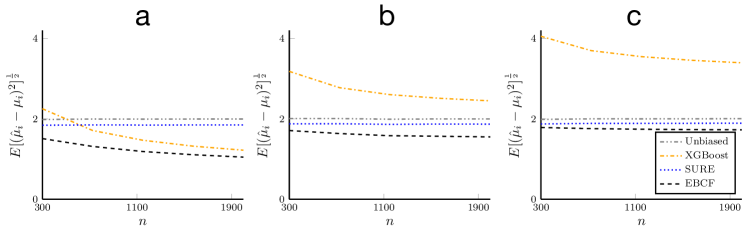
Figure 2: Root mean squared error (RMSE) for estimating $\mu_{i}$ in model (1). Results are shown as a function of $n$ for the four estimators described in the main text. a) Here we let $\sigma=2,A=0$ corresponding to the case of nonparametric regression. In panel b), we let $\sigma=\sqrt{A}=2.0$ corresponding to intermediate shrinkage and in panel c) we let $\sigma=2,\sqrt{A}=3$. The standard errors of all RMSEs are smaller or equal to 0.01.

Synthetic data: We generate data from model (1) with $\mathbb{P}^{X}=U[0,1]^{15}$ and $m(\cdot)$ is the Friedman (1991) function $m(x)=10\sin(\pi x_{1}x_{2})+20(x_{3}-1/2)^{2}+10x_{4}+5x_{5}$, and the last 10 coordinates are noise. Furthermore, we let $\sigma=2.0$ and vary $A\in\left\{0,4,9\right\}$, mimicking the three cases in Figure 1, and we also vary $n$. Results are averaged over 100 simulations and shown in Figure 2. We make the following observation: The unbiased estimator $Z_{i}$ and the SURE estimator which shrinks towards the grand mean have constant mean squared error and results do not improve with increasing $n$. The XGBoost predictor improves with increasing $n$, since $m(\cdot)$ is estimated more accurately; indeed in panel a), if $\hat{m}(\cdot)$ would be exactly equal to $m(\cdot)$, then the error would be $0$. However, as seen in panels $b,c)$, when $A>0$, the mean squared error of XGBoost is lower bounded by $A$, even under perfect prediction of $m(\cdot)$. In contrast, EBCF always improves with $n$ by leveraging the improved predictions of XGBoost, and outperforms all other estimators, even in the case $A=0$ which corresponds to nonparametric regression.

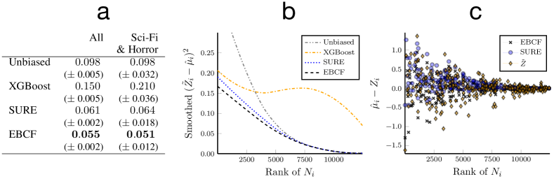
Figure 3: EB analysis of the Movielens dataset for prediction of average movie rating. a) Mean-squared error (MSE) $\smash{n^{-1}\sum_{i=1}^{n}(\hat{\mu}_{i}-\tilde{Z}_{i})^{2}}$ $(\pm\;2\text{ standard errors of the MSE })$ of four estimators for the Movielens dataset (where $\tilde{Z}_{i}$ is the average rating computed from the heldout data with 90% of users) for all movies, as well as the subset of movies that are classified as both Horror and Sci-Fi. b) LOESS smooth of mean squared error across all movies against the rank of $N_{i}$, where $N_{i}$ is the number of users that rated movie $i$ in the training set. c) Deviations of EBCF (empirical Bayes with cross-fitting) and SURE (Stein’s unbiased risk estimate) predictions from the unbiased estimator $Z_{i}$ as a function of $N_{i}$ for all Horror & Sci-Fi movies. We also show the “true” errors $\tilde{Z}_{i}-Z_{i}$.

MovieLens data (Harper and Konstan, 2016): Here we elaborate on the example from the introduction which aims to predict the average movie rating given ratings from a finite number of users. The MovieLens dataset consists of approximately 20 million ratings in $\left\{0,0.5,\dotsc,5\right\}$ from 138,000 users applied to 27,000 movies. To demonstrate the applicability of our approach, when model (1) does not necessarily hold, we randomly choose 10% of all users and attempt to estimate the movie ratings from them. This corresponds to having a much smaller dataset. We then summarize the $i$-th movie, by $Z_{i}$, the average of the $N_{i}$ users (in the training dataset) that rated it. We further have covariates $X_{i}\in\mathbb{R}^{20}$ that include $N_{i}$, the year the movie was released, as well as indicators of 18 genres to which the movie may belong (action, comedy, etc.). We posit that $Z_{i}\mid\mu_{i},X_{i}\sim(\mu_{i},\sigma^{2}/N_{i})$ and want to estimate $\mu_{i}$. As our pseudo ground truth for movie $i$ we use $\tilde{Z}_{i}$, the average movie rating among the remaining $90\%$ of users and then report the error $\sum_{i=1}^{n}(\tilde{Z}_{i}-\hat{\mu}_{i})^{2}/n$, where $n$ is the total number of movies.

The average error across all movies is shown in Figure 3a; here the XGBoost predictor performs worst, followed by the unbiased estimator $Z_{i}$. Instead, the two EB approaches perform a lot better with EBCF scoring the lowest error. The same is true when comparing only the 253 movies with genre tags for both horror and Sci-Fi. In panel b), we show the relationship between the error $(\tilde{Z}_{i}-\hat{\mu}_{i})^{2}$ and the rank of the per-movie number of reviews $N_{i}$ using a LOESS smoother (Cleveland and Devlin, 1988). We observe that the 3 estimators that use $Z_{i}$, do a perfect job for large $N_{i}$ and a worse job for smaller $N_{i}$. In particular, the error of $Z_{i}$ blows up at small $N_{i}$, and the error gains of EBCF occur precisely at low sample sizes. On the other hand, the XGBoost prediction has an error that does not get reduced by larger $N$, but is competitive at small $N$. Panel c) shows $\hat{\mu}_{i}-Z_{i}$ for the 253 predictions of EBCF and SURE for horror/Sci-Fi movies as a function of the rank of $N_{i}$. For large $N_{i}$, again both EB estimators agree with the unbiased estimator. However, for small $N_{i}$, it appears that most Sci-Fi/Horror movies are worse than the average movie, and EB without covariates tries to correct for this by assigning them a higher rating. Conversely, EBCF automatically realizes that these movies tend to get low ratings, and pulls the unbiased estimator $Z_{i}$ further down.

Communities and Crimes data from the UCI repository (Dua and Graff, 2017; Redmond and Baveja, 2002): The dataset provides information about the number of crimes in multiple US communities as compiled by the FBI Uniform Crime Reporting program in 1995. Our task is to predict the non-violent crime rate $p_{i}$ of community $i$, defined as $p_{i}:=\text{Crimes in community }i/\text{Population }i$, for each of $n=2118$ communities. We observe a dataset in which the population of each community is down-sampled to $B=200$ as

$$C_{i}\sim\text{Hypergeometric}(B,\;\text{Crimes in community }i,\;\text{Population }i)$$

We seek to predict $p_{i}$ based on $C_{i}$ and covariates $X_{i}\in\mathbb{R}^{74}$ which include all unnormalized, numeric predictive covariates in the UCI data set description (after removing covariates with missing entries) and comprise features derived from Census and law enforcement data, such as percentage of people that are employed and percentage of police officers assigned to drug units. We note that the hypergeometric subsampling makes the estimation task harder and also provides us with pseudo ground truth $p_{i}$; cf. Wager (2015) for further motivation of such down-sampling.

	$B=200$	$B=500$
	MSE ($\times 10^{6}$)	MSE ($\times 10^{6}$)
Unbiased	$223.9$ ($\pm 16.8$)	$92.2$ ($\pm 7.1$)
XGBoost	$398.0$ ($\pm 81.8$)	$370.2$ ($\pm 78.6$)
SURE	$184.2$ ($\pm 18.9$)	$85.6$ ($\pm 7.2$)
EBCF	$\mathbf{152.0}$ ($\pm 22.2$)	$\mathbf{78.5}$ ($\pm 10.3$)

Table 1: EB analysis of the Communities and Crimes dataset. The table reports the mean-squared error $(\pm\;2\text{ standard errors})$ of four different estimators for the non-violent crime rate. The columns correspond to down-sampling the dataset to a population of ${B=200}$ or $B=500$ for each community.

The problem may be cast into the setting of this paper by defining $Z_{i}:=\sqrt{C_{i}/B}$. Then, by a variance stabilizing argument, it follows that $Z_{i}\mathrel{\dot{\sim}}\left(\sqrt{p_{i}},1/(4\cdot B)\right)$ and we may apply the same methods as in the preceding examples to estimate $\mu_{i}:=\sqrt{p}_{i}$ by $\hat{\mu}_{i}$. After transforming the estimates back to the original scale through $\hat{p}_{i}=\hat{\mu}_{i}^{2}$, we report the error $\sum_{i=1}^{n}(p_{i}-\hat{p}_{i})^{2}/n$, where $n$ is the number of communities analyzed. Table 1 shows the results of this analysis, as well as the same analysis repeated for $B=500$. EBCF shows promising performance compared to the other baselines for both $B$. As we decrease the amount of downsampling from $B=200$ to $B=500$, we see that methods that depend on $Z_{i}$ (unbiased, SURE and EBCF) improve a lot, while XGBoost does not.

6 Discussion

Empirical Bayes is a powerful framework for pooling information across many experiments, and improve the precision of our inference about each experiment on its own (Efron, 2010; Robbins, 1964). Existing empirical Bayes methods, however, do not allow the analyst to leverage covariate information unless they assume a rigid parametric model as in Fay and Herriot (1979), or are willing to commit to a specific end-to-end estimation strategy as in, e.g., Opsomer et al. (2008). In contrast, the approach proposed here allows the analyst to perform covariate-powered empirical Bayes estimation on the basis of any black-box predictive model, and has strong formal properties whether or not the model (1) used to motivate our procedure is well specified. Our approach may be extended in future work by considering generalizations of (1), such as covariate-based modulation of the prior variance, i.e., $\mu_{i}\,\big{|}\,X_{i}\sim\mathcal{N}(m(X_{i}),A(X_{i}))$. The working assumption of a normal prior could also be replaced by heavy-tailed priors (Zhu, Ibrahim, and Love, 2018) or priors with a point mass at zero.

The prevalence of settings where we need to analyze results from many loosely related experiments seems only destined to grow, and we believe that empirical Bayes methods that allow for various forms of structured side information hold promise for fruitful application across several different areas.

Code availability and reproducibility

The proposed EBCF (empirical Bayes with cross-fitting) method has been implemented in EBayes.jl (https://github.com/nignatiadis/EBayes.jl), a package written in the Julia language (Bezanson et al., 2017). Dependencies of EBayes.jl include MLJ.jl (Blaom et al., 2019), Optim.jl (Mogensen and Riseth, 2018) and Distributions.jl (Besançon et al., 2019). We also provide a Github repository (https://github.com/nignatiadis/EBCrossFitPaper) with code to reproduce all empirical results in this paper, including a specification for downloading the dependencies and datasets.

Acknowledgments

The authors are grateful for enlightening conversations with Brad Efron, Guido Imbens, Panagiotis Lolas and Paris Syminelakis. This research was funded by a gift from Google.

Appendix A Proofs for Section 2

A.1 Proof of Theorem 2

Proof.

We will first show, that under model (1), the plug-in estimator (7) satisfies:

$$\mathbb{E}_{m,A}\left[L(\hat{t}_{n};m,A)\right]=\frac{\sigma^{4}}{\left(\sigma^{2}+A\right)^{2}}\mathbb{E}_{m,A}\left[\left(\hat{m}_{n}(X_{n+1})-m(X_{n+1})\right)^{2}\right]$$ (13)

This also establishes the upper bound on the minimax excess risk if $\hat{m}_{n}$ is chosen in a minimax rate-optimal way for the regression problem.

To prove (13), we study the excess risk of this estimator conditionally on the covariate $X_{n+1}$ of the $n+1$-th observation:

$$\mathbb{E}_{m,A}\left[\left(\hat{t}(X_{n+1},Z_{n+1})-\mu_{n+1}\right)^{2}\,\big{|}\,X_{n+1}=x\right]$$

$$= \mathbb{E}_{m,A}\left[\left(\frac{A}{\sigma^{2}+A}Z_{n+1}+\frac{\sigma^{2}}{\sigma^{2}+A}\hat{m}(X_{n+1})-\mu_{n+1}\right)^{2}\,\big{|}\,X_{n+1}=x\right]$$

$$= \mathbb{E}_{m,A}\left[\left(\frac{A}{\sigma^{2}+A}Z_{n+1}+\frac{\sigma^{2}}{\sigma^{2}+A}m(X_{n+1})-\mu_{n+1}+\frac{\sigma^{2}}{\sigma^{2}+A}\left(\hat{m}(X_{n+1})-m(X_{n+1})\right)\right)^{2}\,\big{|}\,X_{n+1}=x\right]$$

$$= \mathbb{E}_{m,A}\left[\left(t^{*}_{m,A}(X_{n+1},Z_{n+1})-\mu_{n+1}\right)^{2}\,\big{|}\,X_{n+1}=x\right]+\frac{\sigma^{4}}{\left(\sigma^{2}+A\right)^{2}}\mathbb{E}_{m,A}\left[\left(\hat{m}(X_{n+1})-m(X_{n+1})\right)^{2}\,\big{|}\,X_{n+1}=x\right]$$

The result follows by integrating over $X_{n+1}$ and rearranging. ∎

A.2 Proof of Lemma 1

The idea of the proof follows the general paradigm in derivation of minimax optimal rates  [Tsybakov, 2008, Duchi, 2019] in which we reduce the original problem to a multiple hypothesis testing problem. More concretely, let us fix two functions $m_{1},m_{2}\in\mathcal{C}$ and call the induced distributions $P_{1}$,$P_{2}$. Say we have a denoiser $t(x,z)$ that performs extremely well under $m_{1}$ with respect to the loss (3). Then we will argue that it cannot do too well under $m_{2}$. But then, given data $(X_{1},Z_{1}),\dotsc,(X_{n},Z_{n})$ we may use the data-driven $\hat{t}(x,z)$ as a proxy for a hypothesis test: If its risk is small under $m_{1}$, but large under $m_{2}$, we would guess that $m_{1}$ is true and vice versa. Thus our task reduces to lower bounding the performance of a hypothesis test. These ideas will be made concrete in the arguments that follow.

Our proof strategy begins by studying the pointwise excess risk:

$$L(t;m,A\mid x):=\mathbb{E}_{m,A}\left[\left(t(x,Z_{n+1})-\mu_{n+1}\right)^{2}-\left(t_{m,A}^{*}(x,Z_{n+1})-\mu_{n+1}\right)^{2}\mid X_{n+1}=x\right]$$ (14)

Lemma 9.

There exist universal constants $c>0,\Delta>0$ such that when $\left\lvert m_{1}(x)-m_{2}(x)\right\rvert/\sqrt{\sigma^{2}+A}\leq\Delta$ (where $x$ is fixed, yet arbitrary) it holds for all $t$ that:

$$\frac{1}{2}\left[L(t;m_{1},A\mid x)+L(t;m_{2},A\mid x)\right]\geq c\frac{\sigma^{4}}{\left(\sigma^{2}+A\right)^{2}}\left(m_{1}(x)-m_{2}(x)\right)^{2}$$

Proof.

As a thought experiment, we consider the following generative model:

$$\mu_{n+1}\;\sim\;G_{x}=\frac{1}{2}\left[\mathcal{N}\left(m_{1}(x),A\right)+\mathcal{N}\left(m_{2}(x),A\right)\right]$$

$$Z_{n+1}\mid\mu_{n+1}\sim\mathcal{N}\left(\mu_{n+1},\sigma^{2}\right)$$

Next consider the Bayes estimator for $\mu_{n+1}$ under this prior, namely:

$$t^{*}_{G_{x}}(z):=\mathbb{E}_{G_{x}}\left[\mu_{n+1}\mid Z_{n+1}=z\right]$$ (15)

Then, by definition of the Bayes estimator, it must hold that for any $t:\mathcal{X}\times\mathbb{R}\to\mathbb{R}$:

$$\mathbb{E}_{G_{x}}\left[\left(t(x,Z_{n+1})-\mu_{n+1}\right)^{2}\right]\geq\mathbb{E}_{G_{x}}\left[\left(t^{*}_{G_{x}}(Z_{n+1})-\mu_{n+1}\right)^{2}\right]$$

In the preceding result we are really thinking of $t$ as the curried function $t(x,\cdot)$. Next, by definition of $G_{x}$, the LHS of the above expression is the same as:

$$\frac{1}{2}\left\{\mathbb{E}_{m_{1},A}\left[\left(t(x,Z_{n+1})-\mu_{n+1}\right)^{2}\mid X_{n+1}=x\right]+\mathbb{E}_{m_{2},A}\left[\left(t(x,Z_{n+1})-\mu_{n+1}\right)^{2}\mid X_{n+1}=x\right]\right\}$$

Also observe that $\inf_{t}\left\{\mathbb{E}_{m_{1},A}\left[\left(t(x,Z_{n+1})-\mu_{n+1}\right)^{2}\mid X_{n+1}=x\right]\right\}=A\sigma^{2}/(A+\sigma^{2})$ and similarly for $m_{2}$, hence upon subtracting $A\sigma^{2}/(A+\sigma^{2})$ from the above expression and its preceding inequality, we get:

$$\frac{1}{2}\left\{L(t;m_{1},A\mid x)+L(t;m_{2},A\mid x)\right\}\geq\mathbb{E}_{G_{x}}\left[\left(t^{*}_{G_{x}}(Z_{n+1})-\mu_{n+1}\right)^{2}\right]-\frac{A\sigma^{2}}{A+\sigma^{2}}$$

Hence to conclude we will need to show that there exist universal constants $c,\Delta>0$ so that if $\left\lvert m_{1}(x)-m_{2}(x)\right\rvert/\sqrt{\sigma^{2}+A}\leq\Delta$:

$$\mathbb{E}_{G_{x}}\left[\left(t^{*}_{G_{x}}(Z_{n+1})-\mu_{n+1}\right)^{2}\right]-\frac{A\sigma^{2}}{A+\sigma^{2}}\;\geq\;c\frac{\sigma^{4}}{\left(\sigma^{2}+A\right)^{2}}\left(m_{1}(x)-m_{2}(x)\right)^{2}$$ (16)

Note that the LHS depends on $m_{1}(x),m_{2}(x)$ through the definition of $G_{x}$. We provide the calculations and complete the proof in Appendix A.3. ∎

Lemma 10.

Let $c>0$, $\Delta>0$ the constants from Lemma 9. Then, for all $m_{1},m_{2}:\mathcal{X}\to\mathbb{R}$, the following implication holds for any $t:\mathcal{X}\times\mathbb{R}\to\mathbb{R}$

$$L(t;m_{1},A)<c\frac{\sigma^{4}}{\left(\sigma^{2}+A\right)^{2}}\int\left(m_{1}(x)-m_{2}(x)\right)^{2}\mathbf{1}\left\{\frac{\left(m_{1}(x)-m_{2}(x)\right)^{2}}{\sigma^{2}+A}\leq\Delta^{2}\right\}d\mathbb{P}^{X}(x)$$ (17)

$$\Longrightarrow L(t;m_{2},A)\geq c\frac{\sigma^{4}}{\left(\sigma^{2}+A\right)^{2}}\int\left(m_{1}(x)-m_{2}(x)\right)^{2}\mathbf{1}\left\{\frac{\left(m_{1}(x)-m_{2}(x)\right)^{2}}{\sigma^{2}+A}\leq\Delta^{2}\right\}d\mathbb{P}^{X}(x)$$

Proof.

We use the result from Lemma (9), noting that $L(t;m,A)=\int L(t;m,A\mid x)d\mathbb{P}^{X}(x)$.

$$\frac{1}{2}\left[L(t;m_{1},A)+L(t;m_{2},A)\right] =\int\frac{1}{2}\left[L(t;m_{1},A\mid x)+L(t;m_{2},A\mid x)\right]d\mathbb{P}^{X}(x)$$

$$\geq\int\frac{1}{2}\left[L(t;m_{1},A\mid x)+L(t;m_{2},A\mid x)\right]\mathbf{1}\left\{\frac{\left(m_{1}(x)-m_{2}(x)\right)^{2}}{\sigma^{2}+A}\leq\Delta^{2}\right\}d\mathbb{P}^{X}(x)$$

$$\geq c\frac{\sigma^{4}}{\left(\sigma^{2}+A\right)^{2}}\int\left(m_{1}(x)-m_{2}(x)\right)^{2}\mathbf{1}\left\{\frac{\left(m_{1}(x)-m_{2}(x)\right)^{2}}{\sigma^{2}+A}\leq\Delta^{2}\right\}d\mathbb{P}^{X}(x)$$

Thus not both $L(t;m_{1},A),L(t;m_{2},A)$ may be $<$ than the RHS at the same time.

∎

The above lemma allows us to prove lower bounds by reduction to hypothesis testing. In particular, let us recall the statement from Lemma 1, now stated in slightly more generality and dropping explicit notation for $n$ in the constructed collection of functions $\left\{m_{v}\mid v\in\mathcal{V}_{n}\right\}$:

Lemma  1 (More general version).

For each $n$, let $\mathcal{V}_{n}$ be a finite set and $\left\{m_{v}\mid v\in\mathcal{V}_{n}\right\}\subset\mathcal{C}$ be a collection of functions indexed by $\mathcal{V}_{n}$ such that for a sequence $\delta_{n}>0$:

$$\delta_{n}^{2}\leq\int\left(m_{v}(x)-m_{v^{\prime}}(x)\right)^{2}\mathbf{1}\left\{\frac{\left(m_{v}(x)-m_{v^{\prime}}(x)\right)^{2}}{\sigma^{2}+A}\leq\Delta^{2}\right\}d\mathbb{P}^{X}(x)\;\text{ for all }v\neq v^{\prime}\in\mathcal{V}_{n},\forall n$$

Then:

$$\mathfrak{M}_{n}^{\text{EB}}\left(\mathcal{C};A,\sigma^{2}\right)\gtrsim\frac{\sigma^{4}}{\left(\sigma^{2}+A\right)^{2}}\cdot\delta^{2}_{n}\cdot\inf_{\hat{V}_{n}}\mathbb{P}\left[\hat{V}_{n}\neq V_{n}\right]$$

Here, $\inf_{\hat{V}_{n}}\mathbb{P}[\hat{V}_{n}\neq V_{n}]$ is to be interpreted as follows: $V_{n}$ is drawn uniformly from $\mathcal{V}_{n}$ and conditionally on $V_{n}=v$, we draw the pairs $(X_{i},Z_{i})_{1\leq i\leq n}$ from model (1) with regression function $m_{n,v}(\cdot)$. The infimum is taken over all estimators $\hat{V}_{n}$ that are measurable with respect to $(X_{i},Z_{i})_{1\leq i\leq n}$.

Note that the original statement of Lemma 1 is subsumed by the above statement. We are ready to prove Lemma 1.

Proof.

Our construction closely follows Duchi [2019] and recent advances in proving minimax results for general losses; see for example [Agarwal et al., 2009]. To start, we fix an estimated denoiser $\hat{t}_{n}(x,z)=\hat{t}_{n}\left(x,z;(X_{i},Z_{i})_{1\leq i\leq n}\right)$ and define $\delta_{n,A,\sigma}=c^{1/2}\frac{\sigma^{2}}{\sigma^{2}+A}\delta_{n}$, where $c$ is defined in Lemma 9. Next, focusing on one $v\in\mathcal{V}$, we get by Markov’s inequality:

$$\mathbb{E}_{m_{v},A}\left[L(\hat{t}_{n};m_{v},A)\right]\geq\delta_{n,A,\sigma}^{2}\mathbb{P}_{m_{v},A}\left[L(\hat{t}_{n};m_{v},A)\geq\delta_{n,A,\sigma}^{2}\right]$$

We next construct an estimator $\tilde{V}_{n}$ of $V_{n}$, namely we let:

$$\tilde{V}_{n}=\operatorname{argmin}_{v\in\mathcal{V}}L(\hat{t}_{n};m_{v},A)$$

Notice that by Lemma 10 and the assumption of the current Lemma, if the truth is $m_{v}$ and $L(\hat{t}_{n};m_{v},A)<\delta_{n,A,\sigma}^{2}$, then we definitely guessed correctly, in other words:

$$L(\hat{t}_{n};m_{v},A)<\delta_{n,A,\sigma}^{2}\;\Longrightarrow\;\tilde{V}_{n}=v$$

But taking the complements:

$$\tilde{V}_{n}\neq v\;\Longrightarrow\;L(\hat{t}_{n};m_{v},A)\geq\delta_{n,A,\sigma}^{2}$$

In terms of probabilities this implies that

$$\mathbb{P}_{m_{v},A}\left[L(\hat{t}_{n};m_{v},A)\geq\delta_{n,A,\sigma}^{2}\right]\geq\mathbb{P}_{m_{v},A}\left[\tilde{V}_{n}\neq v\right]$$

Combining with our original result, and averaging over all $v$, we see that:

$$\sup_{m\in\mathcal{C}}\left\{\mathbb{E}_{m}\left[L(\hat{t}_{n};m,A)\right]\right\} \geq\sup_{v\in\mathcal{V}_{n}}\left\{\mathbb{E}_{m_{v},A}\left[L(\hat{t}_{n};m_{v},A)\right]\right\}$$

$$\geq\frac{1}{\left\lvert\mathcal{V}_{n}\right\rvert}\sum_{v\in\mathcal{V}_{n}}\mathbb{E}_{m_{v},A}\left[L(\hat{t}_{n};m_{v},A)\right]$$

$$\geq\delta_{n,A,\sigma}^{2}\left\{\frac{1}{\left\lvert\mathcal{V}_{n}\right\rvert}\sum_{v\in\mathcal{V}_{n}}P_{m_{v},A}\left[\tilde{V}_{n}\neq v\right]\right\}$$

$$=\delta_{n,A,\sigma}^{2}\mathbb{P}\left[\tilde{V}_{n}\neq V_{n}\right]$$

$$\geq\delta_{n,A,\sigma}^{2}\inf_{\hat{V}_{n}}\mathbb{P}\left[\hat{V}_{n}\neq V_{n}\right]$$

Recall the definition of $\delta_{n,A,\sigma}^{2}$ and that $\hat{t}_{n}$ was arbitrary to conclude. ∎

A.3 Proof of Lemma 9

Proof.

It only remains to prove (16). To this end, let us note that the result is essentially univariate; i.e. we may consider the following model:

$$\mu\;\sim\;G=\frac{1}{2}\left[\mathcal{N}\left(\eta_{1},A\right)+\mathcal{N}\left(\eta_{2},A\right)\right]$$ (18)

$$Z\mid\mu\sim\mathcal{N}\left(\mu,\sigma^{2}\right)$$

In this model, we want to prove that the Bayes risk of the Bayes estimator $t^{*}_{G}(Z)=\mathbb{E}_{G}\left[\mu\mid Z\right]$ satisfies the following inequality ($c>0,\Delta>0$): When $\left\lvert\eta_{1}-\eta_{2}\right\rvert\leq\Delta\sqrt{\sigma^{2}+A}$ it holds that

$$\mathbb{E}_{G}\left[\left(t^{*}_{G}(Z)-\mu\right)^{2}\right]-\frac{A\sigma^{2}}{A+\sigma^{2}}\;\geq\;c\frac{\sigma^{4}}{\left(\sigma^{2}+A\right)^{2}}\left(\eta_{1}-\eta_{2}\right)^{2}$$ (19)

The calculation is facilitated by Lemma 11, which states that $\mathbb{E}_{G}\left[\left(t^{*}_{G}(Z)-\mu\right)^{2}\right]=\sigma^{2}\left[1-\sigma^{2}I(f_{g})\right]$, where $f_{g}$ is the marginal density of $Z$ in (18) and $I(f_{g})$ is the Fisher information $\int\frac{f_{g}^{\prime}(x)^{2}}{f_{g}(x)}dx$.

For the problem at hand, without loss of generality, we may take $\eta_{1}=0$, $\eta_{2}=\eta>0$. Then the marginal distribution induced by $g$ is the mixture $\frac{1}{2}\left[\mathcal{N}\left(0,\sigma^{2}+A\right)+\mathcal{N}\left(\eta,\sigma^{2}+A\right)\right]$, i.e. the pdf $f_{g}(\cdot)$ is:

$$f_{g}(x)=\frac{1}{2\sqrt{2\pi\left(\sigma^{2}+A\right)}}\left[\exp\left(-\frac{x^{2}}{2(\sigma^{2}+A)}\right)+\exp\left(-\frac{(x-\eta)^{2}}{2(\sigma^{2}+A)}\right)\right]$$

$$f_{g}^{\prime}(x)=\frac{1}{2\sqrt{2\pi\left(\sigma^{2}+A\right)}}\frac{1}{\sigma^{2}+A}\left[-x\exp\left(-\frac{x^{2}}{2(\sigma^{2}+A)}\right)-(x-\eta)\exp\left(-\frac{(x-\eta)^{2}}{2(\sigma^{2}+A)}\right)\right]$$

Therefore, letting $\ell(u)=\exp(u)/(1+\exp(u))$ the logistic function, we see that:,

$$\frac{f_{g}^{\prime}(x)}{f_{g}(x)} =\frac{1}{\sigma^{2}+A}\frac{-x-(x-\eta)\exp\left(\frac{-\eta^{2}+2\eta x}{2(\sigma^{2}+A)}\right)}{1+\exp\left(\frac{-\eta^{2}+2\eta x}{2(\sigma^{2}+A)}\right)} =\frac{1}{\sigma^{2}+A}\left[-x+\eta\cdot\ell\left(\frac{-\eta^{2}+2\eta x}{2(\sigma^{2}+A)}\right)\right]$$

Thus:

$$\frac{f_{g}^{\prime}(x)^{2}}{f_{g}(x)^{2}}=\frac{1}{\left(\sigma^{2}+A\right)^{2}}\left[x^{2}+\eta^{2}\cdot\ell^{2}\left(\frac{-\eta^{2}+2\eta x}{2(\sigma^{2}+A)}\right)-2x\eta\cdot\ell\left(\frac{-\eta^{2}+2\eta x}{2(\sigma^{2}+A)}\right)\right]$$

Then, letting $\tilde{x}=x/\sqrt{A+\sigma^{2}}$, $\tilde{\eta}=\eta/\sqrt{A+\sigma^{2}}$:

$$I(f_{g}) =\frac{1}{\left(\sigma^{2}+A\right)^{2}}\frac{1}{2\sqrt{2\pi\left(\sigma^{2}+A\right)}}\int\left\{x^{2}+\eta^{2}\cdot\ell^{2}\left(\frac{-\eta^{2}+2\eta x}{2(\sigma^{2}+A)}\right)-2x\eta\cdot\ell\left(\frac{-\eta^{2}+2\eta x}{2(\sigma^{2}+A)}\right)\right\}$$

$$\qquad\qquad\qquad\qquad\qquad\qquad\qquad\qquad\qquad\cdot\left(\exp\left(-\frac{x^{2}}{2(\sigma^{2}+A)}\right)+\exp\left(-\frac{(x-\eta)^{2}}{2(\sigma^{2}+A)}\right)\right)dx$$

$$=\frac{1}{2\sqrt{2\pi}\left(\sigma^{2}+A\right)}\int\left\{\tilde{x}^{2}+\tilde{\eta}^{2}\cdot\ell^{2}\left(\frac{-\tilde{\eta}^{2}+2\tilde{\eta}\tilde{x}}{2}\right)-2\tilde{x}\tilde{\eta}\cdot\ell\left(\frac{-\tilde{\eta}^{2}+2\tilde{\eta}\tilde{x}}{2}\right)\right\}$$

$$\qquad\qquad\qquad\qquad\qquad\qquad\qquad\qquad\qquad\cdot\left(\exp\left(-\frac{\tilde{x}^{2}}{2}\right)+\exp\left(-\frac{(\tilde{x}-\tilde{\eta})^{2}}{2}\right)\right)d\tilde{x}$$

Thus we may write $I(f_{g})=\frac{1}{\sigma^{2}+A}C(\tilde{\eta})$, for some $C(\tilde{\eta})$, which we now turn to study. Our first observation is that $C(0)=\mathbb{E}\left[\widetilde{X}^{2}\right]=1$ where $\widetilde{X}\sim\mathcal{N}\left(0,1\right)$. We claim that:

$$C(\tilde{\eta})=1-\frac{\tilde{\eta}^{2}}{4}+o(\tilde{\eta}^{2})$$

To this end, we break up $C(\eta)$ into 6 components upon distributing terms, calling them $\mathrm{I}_{0},\mathrm{II}_{0},\mathrm{III}_{0},\mathrm{I}_{\tilde{\eta}},\mathrm{II}_{\tilde{\eta}},\mathrm{III}_{\tilde{\eta}}$, where the subscript corresponds to integrating over $\widetilde{X}\sim\mathcal{N}\left(0,1\right)$ or $\widetilde{X}\sim\mathcal{N}\left(\tilde{\eta},1\right)$.

$$\mathrm{I}_{0}:=\mathbb{E}_{0}\left[\widetilde{X}^{2}\right]=1,\;\;\mathrm{I}_{\tilde{\eta}}:=\mathbb{E}_{\tilde{\eta}}\left[\widetilde{X}^{2}\right]=1+\tilde{\eta}^{2}$$

$$\mathrm{II}_{0}:=\mathbb{E}_{0}\left[\tilde{\eta}^{2}\cdot\ell^{2}\left(\frac{-\tilde{\eta}^{2}+2\tilde{\eta}\widetilde{X}}{2}\right)\right]=\frac{\tilde{\eta}^{2}}{4}+o(\tilde{\eta}^{2})\;\;\;\;\;\;\;\text{ (dominated convergence theorem)}$$

$$\mathrm{II}_{\tilde{\eta}}:=\mathbb{E}_{\tilde{\eta}}\left[\tilde{\eta}^{2}\cdot\ell^{2}\left(\frac{-\tilde{\eta}^{2}+2\tilde{\eta}\widetilde{X}}{2}\right)\right]=\frac{\tilde{\eta}^{2}}{4}+o(\tilde{\eta}^{2})$$

We may see the last result for example as follows, again using dominated convergence ($\tilde{\eta}\to 0$):

$$\frac{\mathrm{II}_{\tilde{\eta}}}{\tilde{\eta}^{2}}=\mathbb{E}_{\tilde{\eta}}\left[\ell^{2}\left(\frac{-\tilde{\eta}^{2}+2\tilde{\eta}\widetilde{X}}{2}\right)\right]=\mathbb{E}_{0}\left[\ell^{2}\left(\frac{-\tilde{\eta}^{2}+2\tilde{\eta}(\widetilde{X}+\tilde{\eta})}{2}\right)\right]=\frac{1}{4}+o(1)$$

To bound $\mathrm{III}$, it will be convenient to note that by Taylor’s theorem it holds that $\ell(u)=\frac{1}{2}+\frac{u}{4}+O(u^{3})$; in fact $\left\lvert\ell(u)-\frac{1}{2}-\frac{u}{4}\right\rvert\leq\left\lvert u\right\rvert^{3}$. Thus:

$$\ell\left(\frac{-\tilde{\eta}^{2}+2\tilde{\eta}\widetilde{X}}{2}\right)=\frac{1}{2}-\frac{\tilde{\eta}^{2}}{8}+\frac{\tilde{\eta}\widetilde{X}}{4}+O\left((-\tilde{\eta}^{2}+2\tilde{\eta}\widetilde{X})^{3}\right)$$

, and so (one may check that again dominated convergence applies):

$$\mathrm{III}_{0}: =-2\tilde{\eta}\mathbb{E}_{0}\left[\widetilde{X}\ell\left(\frac{-\tilde{\eta}^{2}+2\tilde{\eta}\widetilde{X}}{2}\right)\right]=-2\tilde{\eta}\mathbb{E}_{0}\left[\widetilde{X}\left(\frac{1}{2}-\frac{\tilde{\eta}^{2}}{8}+\frac{\tilde{\eta}\widetilde{X}}{4}\right)+O\left(\widetilde{X}(-\tilde{\eta}^{2}+2\tilde{\eta}\widetilde{X})^{3}\right)\right]$$

$$=-2\tilde{\eta}\mathbb{E}_{0}\left[\widetilde{X}\left(\frac{1}{2}-\frac{\tilde{\eta}^{2}}{8}+\frac{\tilde{\eta}\widetilde{X}}{4}\right)\right]+o(\tilde{\eta}^{2})=-2\tilde{\eta}\left(0+\frac{\tilde{\eta}}{4}\right)+o(\tilde{\eta}^{2})=-\frac{\tilde{\eta}^{2}}{2}+o(\tilde{\eta}^{2})$$

$$\mathrm{III}_{\tilde{\eta}}: =-2\tilde{\eta}\mathbb{E}_{\tilde{\eta}}\left[\widetilde{X}\ell\left(\frac{-\tilde{\eta}^{2}+2\tilde{\eta}\widetilde{X}}{2}\right)\right]=-2\tilde{\eta}\mathbb{E}_{\tilde{\eta}}\left[\widetilde{X}\left(\frac{1}{2}-\frac{\tilde{\eta}^{2}}{8}+\frac{\tilde{\eta}\widetilde{X}}{4}\right)+O\left(\widetilde{X}(-\tilde{\eta}^{2}+2\tilde{\eta}\widetilde{X})^{3}\right)\right]$$

$$=-2\tilde{\eta}\mathbb{E}_{0}\left[(\widetilde{X}+\tilde{\eta})\left(\frac{1}{2}-\frac{\tilde{\eta}^{2}}{8}+\frac{\tilde{\eta}(\widetilde{X}+\tilde{\eta})}{4}\right)+O\left((\widetilde{X}+\tilde{\eta})(-\tilde{\eta}^{2}+2\tilde{\eta}(\widetilde{X}+\tilde{\eta}))^{3}\right)\right]$$

$$=-2\tilde{\eta}\mathbb{E}_{0}\left[(\widetilde{X}+\tilde{\eta})\left(\frac{1}{2}-\frac{\tilde{\eta}^{2}}{8}+\frac{\tilde{\eta}(\widetilde{X}+\tilde{\eta})}{4}\right)\right]+o(\tilde{\eta}^{2})$$

$$=-2\tilde{\eta}\left(\frac{\tilde{\eta}}{2}-\frac{\tilde{\eta}^{3}}{8}+\frac{\tilde{\eta}(\tilde{\eta}^{2}+1)}{4}\right)+o(\tilde{\eta}^{2})$$

$$=-\frac{3\tilde{\eta}^{2}}{2}+o(\tilde{\eta}^{2})$$

Add up to get :

$$C(\tilde{\eta})=\frac{1}{2}\left[\mathrm{I}_{0}+\mathrm{II}_{0}+\mathrm{III}_{0}+\mathrm{I}_{\tilde{\eta}}+\mathrm{II}_{\tilde{\eta}}+\mathrm{III}_{\tilde{\eta}}\right]=1-\frac{\tilde{\eta}^{2}}{4}+o(\tilde{\eta}^{2})$$

Then the regret is:

$$\sigma^{2}\left[1-\sigma^{2}I(f_{g})\right]-\frac{A\sigma^{2}}{\sigma^{2}+A} =\sigma^{2}\left(1-\frac{\sigma^{2}}{\sigma^{2}+A}C(\tilde{\eta})\right)-\frac{A\sigma^{2}}{\sigma^{2}+A}$$

$$=\sigma^{2}\left[1-\frac{\sigma^{2}}{\sigma^{2}+A}\left(1-\frac{\tilde{\eta}^{2}}{4}+o(\tilde{\eta}^{2})\right)\right]-\frac{A\sigma^{2}}{\sigma^{2}+A}$$

$$=\frac{\sigma^{4}}{\sigma^{2}+A}\frac{1}{4}\tilde{\eta}^{2}+\frac{\sigma^{4}}{\sigma^{2}+A}o(\tilde{\eta}^{2})$$

$$=\frac{1}{4}\frac{\sigma^{4}}{\left(\sigma^{2}+A\right)^{2}}\eta^{2}+o(\tilde{\eta}^{2})$$

In particular, there exist $c>0,\Delta>0$ such that if $\tilde{\eta}\leq\Delta$:

$$\sigma^{2}\left[1-\sigma^{2}I(f_{g})\right]-\frac{A\sigma^{2}}{\sigma^{2}+A}\geq c\frac{\sigma^{4}}{\left(\sigma^{2}+A\right)^{2}}\eta^{2}$$

Recalling that $\tilde{\eta}=\eta/\sqrt{A+\sigma^{2}}$, we conclude. We also note that we may let $c$ be arbitrarily close to $1/4$.

∎

A.4 Proof and statement of Lemma 11

Lemma 11.

Assume $\mu\sim g$ and $Z\mid\mu\;\sim\;\mathcal{N}\left(\mu,\sigma^{2}\right)$. Also call $f_{g}$ the marginal density of $Z$ and define the Fisher information:

$$I(f_{g}):=\int\frac{f_{g}^{\prime}(x)^{2}}{f_{g}(x)}dx=\mathbb{E}_{f_{g}}\left[\frac{f_{g}^{\prime}(Z)^{2}}{f_{g}(Z)^{2}}\right]$$

Then it holds that:

$$\inf_{\hat{\mu}}\left\{\mathbb{E}_{g}\left[\left(\hat{\mu}-\mu\right)^{2}\right]\right\}=\sigma^{2}\left[1-\sigma^{2}I(f_{g})\right]$$

Remark 12.

This formula is quite well know, see for example [Cohen, Greenshtein, and Ritov, 2013]. Mukhopadhyay and Vidakovic [1995] call it Brown’s formula in light of [Brown, 1971]. We give a proof for completeness; in which we do not justify switching integration and differentiation. For our purposes we only need the result for $g$ a mixture of two normals, in which case this is valid.

Remark 13.

As a simple application, consider $g=\mathcal{N}\left(0,A\right)$, then $f_{g}=\mathcal{N}\left(0,A+\sigma^{2}\right)$, so that $f_{g}(x)=\frac{1}{\sqrt{2\pi\left(\sigma^{2}+A\right)}}\exp\left(-\frac{x^{2}}{2(\sigma^{2}+A)}\right)$ and $f_{g}^{\prime}(x)=-\frac{1}{\sqrt{2\pi\left(\sigma^{2}+A\right)}}\frac{x}{\sigma^{2}+A}\exp\left(-\frac{x^{2}}{2(\sigma^{2}+A)}\right)$. Thus $f_{g}^{\prime}(x)^{2}/f_{g}(x)^{2}=\frac{x^{2}}{\left(\sigma^{2}+A\right)^{2}}$ and $I(f_{g})=\frac{1}{\sigma^{2}+A}$. The above result then states:

$$\inf_{\hat{\mu}}\left\{\mathbb{E}_{g}\left[\left(\hat{\mu}-\mu\right)^{2}\right]\right\}=\sigma^{2}\left[1-\frac{\sigma^{2}}{\sigma^{2}+A}\right]=\frac{\sigma^{2}A}{\sigma^{2}+A}$$

Proof.

We start with noting that the Bayes estimator is given by Tweedie’s [Efron, 2011] celebrated formula:

$$\mathbb{E}_{g}\left[\mu\mid Z=z\right]=z+\sigma^{2}\frac{f_{g}^{\prime}(z)}{f_{g}(z)}$$

Then, the Bayes risk is given by (letting $\varepsilon:=Z-\mu\sim\mathcal{N}\left(0,\sigma^{2}\right)$):

$$\inf_{\hat{\mu}}\left\{\mathbb{E}_{g}\left[\left(\hat{\mu}-\mu\right)^{2}\right]\right\} =\mathbb{E}_{g}\left[\left(\mu-Z-\sigma^{2}\frac{f_{g}^{\prime}(Z)}{f_{g}(Z)}\right)^{2}\right]$$

$$=\mathbb{E}_{g}\left[\left(-\varepsilon-\sigma^{2}\frac{f_{g}^{\prime}(Z)}{f_{g}(Z)}\right)^{2}\right]$$

$$=\sigma^{2}+\sigma^{4}I(f_{g})+2\sigma^{2}\mathbb{E}_{g}\left[\varepsilon\frac{f_{g}^{\prime}(Z)}{f_{g}(Z)}\right]$$

$$=\sigma^{2}-\sigma^{4}I(f_{g})$$

It remains to justify that: $\mathbb{E}_{g}\left[\varepsilon\frac{f_{g}^{\prime}(Z)}{f_{g}(Z)}\right]=-\sigma^{2}I(f_{g})$. To this end, first note that upon conditioning on $\mu$, we may use Stein’s lemma, as follows:

$$\mathbb{E}_{g}\left[\varepsilon\frac{f_{g}^{\prime}(Z)}{f_{g}(Z)}\right] =\mathbb{E}_{g}\left[\mathbb{E}\left[\varepsilon\frac{f_{g}^{\prime}(\varepsilon+\mu)}{f_{g}(\varepsilon+\mu)}\mid\mu\right]\right]$$

$$=\mathbb{E}_{g}\left[\sigma^{2}\mathbb{E}\left[\frac{d}{d\varepsilon}\frac{f_{g}^{\prime}(\varepsilon+\mu)}{f_{g}(\varepsilon+\mu)}\mid\mu\right]\right]$$

$$=\mathbb{E}_{g}\left[\sigma^{2}\left(\frac{f_{g}^{\prime\prime}(Z)}{f_{g}(Z)}-\frac{f_{g}^{\prime}(Z)^{2}}{f_{g}(Z)^{2}}\right)\right]$$

$$=-\sigma^{2}I(f_{g})$$

The last step that remains to be shown is that $\mathbb{E}_{g}\left[\frac{f_{g}^{\prime\prime}(Z)}{f_{g}(Z)}\right]=0$. But this is very similar to a standard Fisher information calculation, in which we interchange integration and differentiation to get that (here $\mu\sim g$):

$$\mathbb{E}_{g}\left[\frac{f_{g}^{\prime\prime}(Z)}{f_{g}(Z)}\right] =\int f_{g}^{\prime\prime}(z)dz=\frac{1}{\sqrt{2\pi\sigma^{2}}}\int\frac{d^{2}}{dz^{2}}\mathbb{E}_{g}\left[\phi((z-\mu)/\sigma)\right]dz=\frac{1}{\sqrt{2\pi\sigma^{2}}}\int\mathbb{E}_{g}\left[\frac{d^{2}}{dz^{2}}\phi((z-\mu)/\sigma)\right]dz$$

$$=\frac{1}{\sqrt{2\pi\sigma^{2}}}\mathbb{E}_{g}\left[\int\frac{d^{2}}{dz^{2}}\phi((z-\mu)/\sigma)dz\right]=0$$

∎

A.5 Local Fano’s Lemma

In this section we provide a Lemma to lower bound the expression $\smash{\inf_{\hat{V}_{n}}\mathbb{P}\left[\hat{V}_{n}\neq V_{n}\right]}$ which appears in Lemma 1. Below, we denote by $\mathbb{P}^{X}\otimes\mathcal{N}\left(m_{v}(\cdot),\;\sigma^{2}+A\right)$ the joint distribution of $(X,Z)$ when $X\sim\mathbb{P}^{X}$ and $Z\mid X\sim\mathcal{N}\left(m_{v}(X),\;\sigma^{2}+A\right)$.

Lemma 14 (Local Fano).

Assume there exists $\kappa>0$ such that for all $v,v^{\prime}\in\mathcal{V}_{n}$:

$$D_{\text{KL}}\left(\mathbb{P}^{X}\otimes\mathcal{N}\left(m_{v}(\cdot),\;\sigma^{2}+A\right)\;\;||\;\;\mathbb{P}^{X}\otimes\mathcal{N}\left(m_{v^{\prime}}(\cdot),\;\sigma^{2}+A\right)\right)\leq\kappa^{2}$$

If also:

$$\log(\left\lvert\mathcal{V}_{n}\right\rvert)\geq 2(n\kappa^{2}+\log(2))$$

Then:

$$\inf_{\hat{V}_{n}}\mathbb{P}\left[\hat{V}_{n}\neq V_{n}\right]\geq\frac{1}{2}$$

Proof.

Let $V_{n}$ uniformly distributed on $\mathcal{V}_{n}$ and $\hat{V}_{n}$ any estimator of $V_{n}$. Then by Fano’s inequality (Corollary 7.9 in Duchi [2019]):

$$\mathbb{P}\left[\hat{V}_{n}\neq V_{n}\right]\geq 1-\frac{I(V_{n};(X_{i},Z_{i})_{1\leq i\leq n})+\log(2)}{\log(\left\lvert\mathcal{V}_{n})\right\rvert}$$

Here $I(V_{n};(X_{i},Z_{i})_{1\leq i\leq n})$ is the mutual information between $V_{n}$ and $(X_{i},Z_{i})_{1\leq i\leq n}$.

Next fix $v,v^{\prime}\in\mathcal{V}_{n}$ and let $P_{v},P_{v^{\prime}}$ the induced distributions of $(X_{1},Z_{1})$ induced by $m_{v}$, resp. $m_{v^{\prime}}$ in model (1), then by (7.4.5) in Duchi [2019]:

$$I(V_{n};(X_{i},Z_{i})_{1\leq i\leq n})\leq\frac{1}{\left\lvert\mathcal{V}\right\rvert^{2}}\sum_{v,v^{\prime}\in\mathcal{V}_{n}}D_{\text{KL}}(P_{v}^{n}||P_{v^{\prime}}^{n})\leq n\max_{v,v^{\prime}\in\mathcal{V}_{n}}D_{\text{KL}}(P_{v}||P_{v^{\prime}})\leq n\kappa^{2}$$

The result follows. ∎

A.6 Fay Herriot results

Proof.

For the upper bound, we will use Theorem 2, where our regression estimator is just the ordinary least squares fit, i.e. $\hat{m}(x)=x^{\top}\hat{\beta}$ with $\hat{\beta}=(X^{\top}X)^{-1}X^{\top}Z_{1:n}$. By $X$ we mean the usual design matrix in which the vectors $X_{1},\dotsc,X_{n}$ are stacked as rows into a matrix.

We start by decomposing the error:

$$\mathbb{E}\left[\left(\hat{m}(X_{n+1})-m(X_{n+1})\right)^{2}\right] =\mathbb{E}\left[\left(X_{n+1}^{\top}\hat{\beta}-X_{n+1}^{\top}\beta\right)^{2}\right]$$

$$=\mathbb{E}\left[\operatorname{tr}\left((\hat{\beta}-\beta)^{\top}X_{n+1}X_{n+1}^{\top}(\hat{\beta}-\beta)\right)\right]$$

$$=\mathbb{E}\left[\operatorname{tr}\left((\hat{\beta}-\beta)(\hat{\beta}-\beta)^{\top}X_{n+1}X_{n+1}^{\top}\right)\right]$$

$$=\operatorname{tr}\left(\mathbb{E}\left[(\hat{\beta}-\beta)(\hat{\beta}-\beta)^{\top}\right]\Sigma\right)$$

Hence recalling that $\mathbb{E}\left[\hat{\beta}\right]=\beta$, we only need to study the covariance of $\hat{\beta}$.

$$\operatorname{Cov}\left[\hat{\beta}\right] =\mathbb{E}\left[\operatorname{Cov}\left[\hat{\beta}\mid X_{1:n}\right]\right]\;\;+\;\;\operatorname{Cov}\left[\mathbb{E}\left[\hat{\beta}\mid X_{1:n}\right]\right]$$

$$=(\sigma^{2}+A)\mathbb{E}\left[\left(X^{\top}X\right)^{-1}\right]\;\;+\;\;0$$

$$=(\sigma^{2}+A)\Sigma^{-1}\frac{1}{n-d-1}$$

The last equality holds because $X^{\top}X$ follows a Wishart distribution. See Theorem 2 in Rosset and Tibshirani [2018] and references therein for similar results. In total we get:

$$\mathbb{E}\left[\left(\hat{m}(X_{n+1})-m(X_{n+1})\right)^{2}\right]=\operatorname{tr}\left((\sigma^{2}+A)\Sigma^{-1}\frac{1}{n-d-1}\Sigma\right)=\frac{d(\sigma^{2}+A)}{n-p-1}$$

For the lower bound, we will apply Lemma 1. First we let $\mathcal{V}_{n}$ be an $1/2$ packing of the Euclidean ($\ell_{2}$) unit ball which has cardinality at least $2^{d}$ (Lemma 7.6. in Duchi [2019])

Then, for $v\in V_{n}$ we define $\theta_{v}=\varepsilon v$ (we will specify $\varepsilon$ later). Then we let $\beta_{v}=\Sigma^{-1/2}\theta_{v}$ and note that for two distinct $v,v^{\prime}$:

$$\mathbb{E}\left[\left(X_{n+1}^{\top}\beta_{v}-X_{n+1}^{\top}\beta_{v^{\prime}}\right)^{2}\right] =\operatorname{tr}\left(\mathbb{E}\left[(\beta_{v}-\beta_{v^{\prime}})(\beta_{v}-\beta_{v^{\prime}})^{\top}\right]\Sigma\right)$$

$$=\operatorname{tr}\left(\mathbb{E}\left[\Sigma^{-1/2}(\theta_{v}-\theta_{v^{\prime}})(\theta_{v}-\theta_{v^{\prime}})^{\top}\Sigma^{-1/2}\right]\Sigma\right)$$

$$=\mathbb{E}\left[\left\lVert\theta_{v}-\theta_{v^{\prime}}\right\rVert^{2}_{2}\right]$$

$$\geq\frac{\varepsilon^{2}}{4}$$

In the last step we used the packing property of the set $\mathcal{V}_{n}$ we defined.

On the other hand:

$$D_{\text{KL}}\left(\mathcal{N}\left(0,\Sigma\right)\otimes\mathcal{N}\left(\langle\cdot,\beta_{v}\rangle,\;\sigma^{2}+A\right)\;\;||\;\;\mathcal{N}\left(0,\Sigma\right)\otimes\mathcal{N}\left(\langle\cdot,\beta_{v^{\prime}}\rangle,\;\sigma^{2}+A\right)\right)$$

$$= \mathbb{E}\left[D_{\text{KL}}\left(\mathcal{N}\left(X_{n+1}^{\top}\beta_{v},\sigma^{2}+A\right)\;\;||\;\;\mathcal{N}\left(X_{n+1}^{\top}\beta_{v^{\prime}},\sigma^{2}+A\right)\,\big{|}\,X_{n+1}\right)\right]$$

$$= \mathbb{E}\left[\frac{1}{2(A+\sigma^{2})}\left(X_{n+1}^{\top}\beta_{v}-X_{n+1}^{\top}\beta_{v^{\prime}}\right)^{2}\right]$$

$$= \frac{1}{2(A+\sigma^{2})}\mathbb{E}\left[\left\lVert\theta_{v}-\theta_{v^{\prime}}\right\rVert^{2}_{2}\right]$$

$$\leq \frac{2\varepsilon^{2}}{A+\sigma^{2}}$$

To apply Lemma 14 we need the following to hold for a constant $C$:

$$\log(2^{d})\geq C\frac{n\varepsilon^{2}}{A+\sigma^{2}}$$

So we may pick $\varepsilon^{2}=c\frac{d(A+\sigma^{2})}{n}$ for a constant $c$. Since $\varepsilon\to 0$ as $n\to\infty$, we may apply Lemma 1 for large enough $n$ with separation say $\varepsilon^{2}/10$, by which we can conclude. ∎

A.7 Lipschitz results

Proof.

The upper bound follows from Theorem 2, where the regressor $\hat{m}_{n}$ is the $k$-nearest neighbor regression predictor (KNN) with optimally tuned number of neighbors, see Theorem 6.2 and Problem 6.7 in Györfi et al. [2006].

For the lower bound, we will apply Lemma 1. To this end, we start by constructing $\mathcal{V}_{n}$ as in the proof of Theorem 3.2. in Györfi et al. [2006]: We define $M_{n}\in\mathbb{N}$ and partition $[0,1]^{d}$ (we will pick $M_{n}$ later) into $M_{n}^{d}$ cubes $A_{n,j}$ of side length $1/M_{n}$ and with centers $a_{n,j}$. Next we take any function $\bar{m}:\mathbb{R}^{d}\to\mathbb{R}$ which is $1$-Lipschitz, vanishes outside $[-\frac{1}{2},\frac{1}{2}]^{d}$ and $C_{I}:=\int\bar{m}^{2}(x)dx>0$. We also define $\bar{m}_{L}(\cdot)=L\cdot\bar{m}(\cdot)$. Finally, for $j=1,\dotsc,M_{n}^{d}$ we define:

$$\bar{m}_{L,n,j}(x)=\frac{1}{M_{n}}\bar{m}_{L}(M_{n}(x-a_{n,j}))$$

Then we let $\mathcal{V}_{n}\subset\left\{\pm 1\right\}^{M_{n}^{d}}$ with $\left\lvert\mathcal{V}_{n}\right\rvert\geq\exp(M_{n}^{d}/8)$ and so that for all $v,v^{\prime}\in\mathcal{V}_{n}$:

$$\sum_{j=1}^{M_{n}^{d}}\mathbf{1}\left(v_{j}\neq v_{j}^{\prime}\right)\geq\frac{M_{n}^{d}}{4}$$

Such a set exists by the Gilbert-Varshamov bound (Lemma 7.5 in Duchi [2019]). With $\mathcal{V}_{n}$ in hand, we define for $v\in\mathcal{V}_{n}$:

$$m_{v}(x)=\sum_{j=1}^{M_{n}^{d}}v_{j}\bar{m}_{L,n,j}(x)$$

We argue that $m_{v}(x)$ indeed is $L$-Lipschitz: All $\bar{m}_{L,n,j}$ are $L$-Lipschitz, since so is $\bar{m}_{L}$ and furthermore observe that all $\bar{m}_{L,n,j},\;j=1,\dotsc,M_{n}^{d}$ have disjoint support.

Next, take $v\neq v^{\prime}\in\mathcal{V}_{n}$. Then, since the $\bar{m}_{L,n,j}$ have disjoint support:

$$\int\left(m_{v}(x)-m_{v^{\prime}}(x)\right)^{2}d\mathbb{P}^{X}(x) =\sum_{j=1}^{M_{n}^{d}}(v_{j}-v_{j}^{\prime})^{2}\int\bar{m}_{L,n,j}^{2}(x)d\mathbb{P}^{X}(x)$$

$$\geq\sum_{j=1}^{M_{n}^{d}}(v_{j}-v_{j}^{\prime})^{2}\eta\int\bar{m}_{L,n,j}^{2}dx$$

$$=\sum_{j=1}^{M_{n}^{d}}(v_{j}-v_{j}^{\prime})^{2}\frac{\eta L^{2}}{M_{n}^{2+d}}C_{I}$$

$$=\frac{4\eta L^{2}}{M_{n}^{2+d}}C_{I}\sum_{j=1}^{M_{n}^{d}}\mathbf{1}\left(v_{j}\neq v_{j}^{\prime}\right)$$

$$\geq\frac{4\eta L^{2}}{M_{n}^{2+d}}C_{I}\frac{M_{n}^{d}}{4}=\eta C_{I}\frac{L^{2}}{M_{n}^{2}}$$

On the other hand, let us bound the KL divergence between the distributions induced by $m_{v},m_{v^{\prime}}$:

$$D_{\text{KL}}\left(\mathbb{P}^{X}\otimes\mathcal{N}\left(m_{v}(\cdot),\;\sigma^{2}+A\right)\;\;||\;\;\mathbb{P}^{X}\otimes\mathcal{N}\left(m_{v^{\prime}}(\cdot),\;\sigma^{2}+A\right)\right)$$

$$= \mathbb{E}\left[D_{\text{KL}}\left(\mathcal{N}\left(m_{v}(X_{n+1}),\;\sigma^{2}+A\right)\;\;||\;\;\mathcal{N}\left(m_{v^{\prime}}(X_{n+1}),\;\sigma^{2}+A\right)\mid X_{n+1}\right)\right]$$

$$= \int\frac{1}{2(\sigma^{2}+A)}\left(m_{v}(x)-m_{v^{\prime}}(x)\right)^{2}d\mathbb{P}^{X}(x)$$

$$\leq \frac{1}{2\eta(\sigma^{2}+A)}\int\left(m_{v}(x)-m_{v^{\prime}}(x)\right)^{2}dx$$

$$\leq \frac{1}{2\eta(\sigma^{2}+A)}\frac{4L^{2}}{M_{n}^{2+d}}C_{I}\sum_{j=1}^{M_{n}^{d}}\mathbf{1}\left(v_{j}\neq v_{j}^{\prime}\right)$$

$$\leq \frac{2C_{I}}{\eta(\sigma^{2}+A)}\frac{L^{2}}{M_{n}^{2}}$$

Next, we will lower bound $\inf_{\hat{V}_{n}}\mathbb{P}\left[\hat{V}_{n}\neq V_{n}\right]$ by Lemma 14. To get the condition, we need that for some $C>0$:

$$M_{n}^{d}\geq C\frac{L^{2}n}{(\sigma^{2}+A)M_{n}^{2}}\;\Leftrightarrow M_{n}\geq C\left(\frac{L^{2}n}{\sigma^{2}+A}\right)^{\frac{1}{2+d}}$$

Hence for some $C$, we set $M_{n}=\lceil C\left(\frac{L^{2}n}{\sigma^{2}+A}\right)^{\frac{1}{2+d}}\rceil$. Then the separation between two hypotheses $m_{v},m_{v^{\prime}}$ is equal to (for another constant $C^{\prime}$):

$$\int\left(m_{v}(x)-m_{v^{\prime}}(x)\right)^{2}d\mathbb{P}^{X}(x)\geq\eta C_{I}\frac{L^{2}}{M_{n}^{2}}\geq C^{\prime}\left(\frac{L^{d}(\sigma^{2}+A)}{n}\right)^{\frac{2}{2+d}}$$

We conclude by Lemma 1 upon noting that $M_{n}\to\infty$ and hence $\sup_{v\in\mathcal{V}_{n}}\sup_{x}\left\lvert m_{v}(x)\right\rvert\to 0$ as $n\to\infty$.

∎

Appendix B Results for sample-split EB in Section 3

in Section 3 we made the following point: Even if we knew the true $A$, it would not be the optimal $A$ to plug into (7). We formalize this in the following proposition:

Proposition 15.

Consider model (1). Fix any (deterministic) function $\tilde{m}:\mathcal{X}\to\mathbb{R}$ and define:

$$A_{\tilde{m}}:=\mathbb{E}_{m,A}\left[\left(\tilde{m}(X_{n+1})-Z_{n+1}\right)^{2}\right]-\sigma^{2}$$ (20)

Then:

$$\mathbb{E}_{m,A}\left[\left(t^{*}_{\tilde{m},A_{\tilde{m}}}(X_{n+1},Z_{n+1})-\mu_{n+1}\right)^{2}\right]=\inf_{\tilde{A}\geq 0}\mathbb{E}_{m,A}\left[\left(t^{*}_{\tilde{m},\tilde{A}}(X_{n+1},Z_{n+1})-\mu_{n+1}\right)^{2}\right]$$

The above expressions are equal to: $\frac{\sigma^{2}A_{\tilde{m}}}{\sigma^{2}+A_{\tilde{m}}}$. Furthermore, a direct consequence is that:

$$\mathbb{E}_{m,A}\left[\left(t^{*}_{\tilde{m},A_{\tilde{m}}}(X_{n+1},Z_{n+1})-\mu_{n+1}\right)^{2}\right]\leq\mathbb{E}_{m,A}\left[\left(t^{*}_{\tilde{m},A}(X_{n+1},Z_{n+1})-\mu_{n+1}\right)^{2}\right]$$

Proof.

Let us consider the following class of shrinkage rules, where $\lambda\in[0,1]$:

$$t_{\lambda}(x,z)=\lambda\tilde{m}(x)+(1-\lambda)z=\lambda\left(\tilde{m}(x)-z\right)+z$$

Then our goal will be to minimize the following function over $\lambda\in[0,1]$:

$$J(\lambda)=\mathbb{E}_{m,A}\left[\left(t_{\lambda}(X_{n+1},Z_{n+1})-\mu_{n+1}\right)^{2}\right]$$ (21)

To this end:

$$J(\lambda) =\mathbb{E}_{m,A}\left[\left\{t_{\lambda}(X_{n+1},Z_{n+1})-\mu_{n+1}\right\}^{2}\right]$$

$$=\mathbb{E}_{m,A}\left[\left\{\lambda\left(\tilde{m}(X_{n+1})-Z_{n+1}\right)+Z_{n+1}-\mu_{n+1}\right\}^{2}\right]$$

$$=\lambda^{2}\mathbb{E}_{m,A}\left[\left(\tilde{m}(X_{n+1})-Z_{n+1}\right)^{2}\right]+2\lambda\mathbb{E}_{m,A}\left[\left(\tilde{m}(X_{n+1})-Z_{n+1}\right)\left(Z_{n+1}-\mu_{n+1}\right)\right]+\sigma^{2}$$

$$=\lambda^{2}\mathbb{E}_{m,A}\left[\left(\tilde{m}(X_{n+1})-Z_{n+1}\right)^{2}\right]-2\lambda\sigma^{2}+\sigma^{2}$$

The last step follows from the two following intermediate results:

$$\mathbb{E}_{m,A}\left[\tilde{m}(X_{n+1})\left(Z_{n+1}-\mu_{n+1}\right)\right]=\mathbb{E}_{m,A}\left[\tilde{m}(X_{n+1})\mathbb{E}_{m,A}\left[Z_{n+1}-\mu_{n+1}\mid X_{n+1}\right]\right]=0$$

$$\mathbb{E}_{m,A}\left[Z_{n+1}\left(Z_{n+1}-\mu_{n+1}\right)\right]=\mathbb{E}_{m,A}\left[\operatorname{Var}_{m,A}\left[Z_{n+1}\mid\mu_{n+1}\right]\right]=\sigma^{2}$$

We may now directly minimizer over $A$ to see that the optimal $\lambda$ is given by:

$$\lambda^{*}(\tilde{m})=\frac{\sigma^{2}}{\mathbb{E}_{m,A}\left[\left(\tilde{m}(X_{n+1})-Z_{n+1}\right)^{2}\right]}$$

The form of $A_{\tilde{m}}$ then directly follows by noting the one-to-one correspondence $\lambda\leftrightarrow\frac{\sigma^{2}}{A_{\tilde{m}}+\sigma^{2}}$. ∎

We will now prove that for deterministic $\tilde{m}$, as in Proposition 15, parametric rates are possible in the estimation of $A_{\tilde{m}}$, which translate into $O(1/n)$ decay of the regret.

Proposition 16.

Consider $n$ i.i.d. observations $(X_{i},Z_{i})$ from model (1) with $A,\sigma>0$. Fix any (deterministic) function $\tilde{m}:\mathcal{X}\to\mathbb{R}$ with $\mathbb{E}\left[\tilde{m}(X_{n+1})^{4}\right]\leq M$ for some $M<\infty$ (here $X_{n+1}\sim\mathbb{P}^{X}$). Let:

$$\hat{A}_{n}=\left(\frac{1}{n}\sum_{k=1}^{n}\left(\tilde{m}(X_{k})-Z_{k}\right)^{2}-\sigma^{2}\right)_{+}$$

Then $\hat{t}_{n}=t^{*}_{\tilde{m},\hat{A}_{n}}$ satisfies:

$$\mathbb{E}_{m,A}\left[L\left(\hat{t}_{n};m,A\right)\right]\leq\mathbb{E}_{m,A}\left[L(t^{*}_{\tilde{m},A_{\tilde{m}}};m,A)\right]+O(1/n)$$

Thus also:

$$\mathbb{E}_{m,A}\left[L\left(\hat{t}_{n};m,A\right)\right]\leq\mathbb{E}_{m,A}\left[L(t^{*}_{\tilde{m},A};m,A)\right]+O(1/n)$$

Proof.

We consider again the $J(\lambda)$ from (21) and recall that $J(\lambda^{*}(\tilde{m}))=\min_{\lambda\geq 0}J(\lambda)$. We note that $J(\lambda)$ is a convex quadratic in $\lambda$ with:

$$J^{\prime}(\lambda)=2\lambda\mathbb{E}_{m,A}\left[\left(\tilde{m}(X_{n+1})-Z_{n+1}\right)^{2}\right]-2\sigma^{2},\;\;J^{\prime\prime}(\lambda)=2\mathbb{E}_{m,A}\left[\left(\tilde{m}(X_{n+1})-Z_{n+1}\right)^{2}\right]$$

Thus, since $J^{\prime}(\lambda^{*}(\tilde{m}))=0$, we get for any $\lambda$:

$$J(\lambda)=J(\lambda^{*}(\tilde{m}))+\mathbb{E}_{m,A}\left[\left(\tilde{m}(X_{n+1})-Z_{n+1}\right)^{2}\right]\left(\lambda-\lambda^{*}(\tilde{m})\right)^{2}$$

This means that:

$$L(t_{\lambda};m,A)=L(t_{\lambda^{*}(\tilde{m})};m,A)+\mathbb{E}_{m,A}\left[\left(\tilde{m}(X_{n+1})-Z_{n+1}\right)^{2}\right]\left(\lambda-\lambda^{*}(\tilde{m})\right)^{2}$$

Hence to conclude we will need to bound $\mathbb{E}_{m,A}\left[\left(\hat{\lambda}_{n}-\lambda^{*}(\tilde{m})\right)^{2}\right]$, where:

$$\hat{\lambda}_{n}=\frac{\sigma^{2}}{\sigma^{2}\lor\left(\frac{1}{n}\sum_{k=1}^{n}\left(\tilde{m}(X_{k})-Z_{k}\right)^{2}\right)}$$

Using the fact that both $\sigma^{2}\lor\left(\frac{1}{n}\sum_{k=1}^{n}\left(\tilde{m}(X_{k})-Z_{k}\right)^{2}\right)$ and $\mathbb{E}_{m,A}\left[\left(\tilde{m}(X_{k})-Z_{k}\right)^{2}\right]$ are $\geq\sigma^{2}$ and Taylor’s theorem applied to $u\mapsto 1/u$, we get:

$$\mathbb{E}_{m,A}\left[\left(\hat{\lambda}-\lambda^{*}(\tilde{m})\right)^{2}\right] =\sigma^{4}\mathbb{E}_{m,A}\left[\left(\frac{1}{\sigma^{2}\lor\left(\frac{1}{n}\sum_{k=1}^{n}\left(\tilde{m}(X_{k})-Z_{k}\right)^{2}\right)}-\frac{1}{\mathbb{E}_{m,A}\left[\left(\tilde{m}(X_{k})-Z_{k}\right)^{2}\right]}\right)^{2}\right]$$

$$\leq \mathbb{E}_{m,A}\left[\left(\sigma^{2}\lor\left(\frac{1}{n}\sum_{k=1}^{n}\left(\tilde{m}(X_{k})-Z_{k}\right)^{2}\right)-\mathbb{E}_{m,A}\left[\left(\tilde{m}(X_{k})-Z_{k}\right)^{2}\right]\right)^{2}\right]$$

$$\leq \mathbb{E}_{m,A}\left[\left(\frac{1}{n}\sum_{k=1}^{n}\left(\tilde{m}(X_{k})-Z_{k}\right)^{2}-\mathbb{E}_{m,A}\left[\left(\tilde{m}(X_{k})-Z_{k}\right)^{2}\right]\right)^{2}\right]$$

$$= \operatorname{Var}_{m,A}\left[\frac{1}{n}\sum_{k=1}^{n}\left(\tilde{m}(X_{k})-Z_{k}\right)^{2}\right]$$

$$= \frac{1}{n}\operatorname{Var}_{m,A}\left[\left(\tilde{m}(X_{k})-Z_{k}\right)^{2}\right]$$

This is $O(1/n)$ as long as $\operatorname{Var}_{m,A}\left[\left(\tilde{m}(X_{k})-Z_{k}\right)^{2}\right]$ is upper bounded, which is the case under the given assumptions. The last statement follows from Proposition 15.

∎

We are now in a position to prove Theorem 5

Theorem 5.

We apply Proposition 16 for the data in fold $I_{2}$ conditionally on the first fold, i.e. conditionally on $Z_{I_{1}},\mu_{I_{1}},X_{I_{1}}$. ∎

Appendix C Results under misspecification

C.1 Proof of Theorem 6 (James-Stein property)

Before proceeding with the proof, let us introduce the following lemma:

Lemma 17.

Fix $\nu\in\mathbb{N}$, a fixed vector $\xi=(\xi_{1},\dotsc,\xi_{\nu})$, a mean vector $\theta=(\theta_{1},\dotsc,\theta_{\nu})$ and independent $Y_{1},\dotsc,Y_{\nu}$ distributed as $Y_{i}\sim\mathcal{N}\left(\theta_{i},\sigma^{2}\right)$. Then consider the following positive-part James-Stein type estimator, parametrized by $a>0$:

$$\hat{\theta}_{a}=\xi+\left(1-\frac{a\sigma^{2}}{\left\lVert Y-\xi\right\rVert_{2}^{2}}\right)_{+}\left(Y-\xi\right)$$ (22)

This estimator has risk:

$$\mathbb{E}\left[\left\lVert\hat{\theta}_{a}-\theta\right\rVert^{2}_{2}\right]\leq\nu\sigma^{2}-a\sigma^{2}\left[2(\nu-2)-a\right]\mathbb{E}\left[\frac{\sigma^{2}}{\left\lVert Y-\xi\right\rVert_{2}^{2}}\right]$$ (23)

In particular, if $\nu\geq 5$ (resp. $\nu\geq 3$), $\hat{\theta}_{\nu}$ (resp. $\hat{\theta}_{\nu-2}$) has squared error risk $<\nu\sigma^{2}$.

Proof.

Estimator (22) where we do not take the positive part of $\left(1-\frac{a\sigma^{2}}{\left\lVert Y-\xi\right\rVert_{2}^{2}}\right)_{+}$ has risk precisely equal to the RHS in (23). This is well known, see for example Lemma 1 in [Green and Strawderman, 1991] and references therein. The positive part estimator then has smaller risk, as also follows from well known results on James-Stein estimation, see e.g. [Baranchik, 1964]. Finally when $a=\nu\geq 5$, $a\sigma^{2}\left[2(\nu-2)-a\right]=\sigma^{2}\left[\nu-4\right]>0$. ∎

We are ready to prove Theorem 6:

Proof.

Let $\widetilde{\mathbb{P}}_{I_{1}}\left[\;\cdot\;\right]=\mathbb{P}\left[\;\cdot\mid Z_{I_{1}},\mu_{1:n},X_{1:n}\right]$. Then w.r.t. $\widetilde{\mathbb{P}}_{I_{1}}\left[\cdot\right]$, it holds that $(Z_{i})_{i\in I_{2}}$ are independent and $Z_{i}\sim\mathcal{N}\left(\mu_{i},\sigma^{2}\right)$ for $i\in I_{2}$. Furthermore $\hat{m}_{I_{1}}(X_{I_{2}})=(\hat{m}_{I_{1}}(X_{i}))_{i\in I_{2}}$ is deterministic w.r.t. $\widetilde{\mathbb{P}}_{I_{1}}\left[\cdot\right]$ and also recall that:

$$\hat{\mu}_{I_{2}}^{\text{EBCF}} =\frac{\sigma^{2}}{\hat{A}_{I_{2}}+\sigma^{2}}\hat{m}_{I_{1}}(X_{I_{2}})+\frac{\hat{A}_{I_{2}}}{\hat{A}_{I_{2}}+\sigma^{2}}Z_{I_{2}}$$

$$=\hat{m}_{I_{1}}(X_{I_{2}})+\left(1-\frac{\sigma^{2}}{\hat{A}_{I_{2}}+\sigma^{2}}\right)\left(Z_{I_{2}}-\hat{m}_{I_{1}}(X_{I_{2}})\right)$$

Also from (8) it holds that:

$$\hat{A}_{I_{2}}=\left(\frac{1}{\left\lvert I_{2}\right\rvert}\sum_{i\in I_{2}}\left(\hat{m}_{I_{1}}(X_{i})-Z_{i}\right)^{2}-\sigma^{2}\right)_{+}$$

Thus $\hat{\mu}_{I_{2}}$ takes precisely the form from (22) with $a=\left\lvert I_{2}\right\rvert$ and thus applying Lemma 17 (w.r.t. $\widetilde{\mathbb{P}}_{I_{1}}\left[\;\cdot\;\right]$, also by assumption $\left\lvert I_{2}\right\rvert\geq 5$), we get:

$$\sum_{i\in I_{2}}\widetilde{\mathbb{E}}_{I_{1}}\left[\left(\mu_{i}-\hat{\mu}_{i}^{\text{EBCF}}\right)^{2}\right]<\sum_{i\in I_{2}}\widetilde{\mathbb{E}}_{I_{1}}\left[(\mu_{i}-Z_{i})^{2}\right]=\left\lvert I_{2}\right\rvert\sigma^{2}$$

Integrate w.r.t. $Z_{I_{1}}$, to get:

$$\sum_{i\in I_{2}}\mathbb{E}\left[\left(\mu_{i}-\hat{\mu}_{i}^{\text{EBCF}}\right)^{2}\,\big{|}\,\mu_{1:n},X_{1:n}\right]<\left\lvert I_{2}\right\rvert\sigma^{2}$$

Now apply the symmetric argument with the folds flipped to also get:

$$\sum_{i\in I_{1}}\mathbb{E}\left[\left(\mu_{i}-\hat{\mu}_{i}^{\text{EBCF}}\right)^{2}\,\big{|}\,\mu_{1:n},X_{1:n}\right]<\left\lvert I_{1}\right\rvert\sigma^{2}$$

Add both inequalities and divide by $n$ to conclude. ∎

C.2 SURE results

Below we prove Theorem 7. Throughout the proof we deal with the more general case of unequal variances. In particular, we replace the assumption that $(X_{i},Z_{i})$ satisfy (9) by the following model (while keeping all other assumptions):

$$(X_{i},\mu_{i})\sim\mathbb{P}^{(X_{i},\mu_{i})},\;\;Z_{i}\mid\mu_{i},X_{i}\sim\left(\mu_{i},\sigma_{i}^{2}\right),\;\text{ i.e. }\mathbb{E}\left[Z_{i}\mid\mu_{i},X_{i}\right]=\mu_{i},\;\operatorname{Var}\left[Z_{i}\mid\mu_{i},X_{i}\right]=\sigma_{i}^{2}$$

Theorem 7.

Our proof closely follows Xie et al. [2012]. Let $n_{2}=\left\lvert I_{2}\right\rvert$. We also use the same notation as in the proof of Theorem 6, wherein $\widetilde{\mathbb{P}}_{I_{1}}\left[\;\cdot\;\right]=\mathbb{P}\left[\;\cdot\mid Z_{I_{1}},\mu_{1:n},X_{1:n}\right]$. For $i\in I_{2}$ we also write $\tilde{m}_{i}=\hat{m}_{I_{1}}(X_{i})$. We rewrite the $\operatorname{SURE}$ expression as follows:

$$\operatorname{SURE}_{I_{2}}(A)=\frac{1}{n_{2}}\sum_{i\in I_{2}}\left(\sigma_{i}^{2}+\frac{\sigma_{i}^{4}}{(A+\sigma_{i}^{2})^{2}}(Z_{i}-\tilde{m}_{i})^{2}-2\frac{\sigma_{i}^{4}}{A+\sigma_{i}^{2}}\right)=\frac{1}{n_{2}}\sum_{i\in I_{2}}\left[\frac{\sigma_{i}^{4}}{(A+\sigma_{i}^{2})^{2}}(Z_{i}-\tilde{m}_{i})^{2}+\frac{\sigma_{i}^{2}(A-\sigma_{i}^{2})}{A+\sigma_{i}^{2}}\right]$$

We also define $\ell_{I_{2}}(A)$, the average loss in fold $I_{2}$ when we estimate $\mu_{i}$ by $t^{*}_{\hat{m}_{I_{1}},A}(X_{i},Z_{i})$, i.e.:

$$\ell_{I_{2}}(A):=\frac{1}{n_{2}}\sum_{i\in I_{2}}\left(\mu_{i}-t^{*}_{\hat{m}_{I_{1}},A}(X_{i},Z_{i})\right)^{2}$$

Next we collect the difference between the SURE risk estimate and the actual loss:

$$\operatorname{SURE}_{I_{2}}(A)-\ell_{I_{2}}(A) =\frac{1}{n_{2}}\sum_{i\in I_{2}}\left[\left(\frac{\sigma_{i}^{4}}{(A+\sigma_{i}^{2})^{2}}(Z_{i}-\tilde{m}_{i})^{2}+\frac{\sigma_{i}^{2}(A-\sigma_{i}^{2})}{A+\sigma_{i}^{2}}\right)-\left(\mu_{i}-\frac{A}{A+\sigma_{i}^{2}}Z_{i}-\frac{\sigma_{i}^{2}}{A+\sigma_{i}^{2}}\tilde{m}_{i}\right)^{2}\right]$$

$$=\frac{1}{n_{2}}\sum_{i\in I_{2}}\left\{\left[\left(Z_{i}-\tilde{m}_{i}\right)^{2}-\sigma_{i}^{2}-\left(\mu_{i}-\tilde{m}_{i}\right)^{2}\right]-\frac{2A}{A+\sigma_{i}^{2}}\left[\left(Z_{i}-\tilde{m}_{i}\right)^{2}-(Z_{i}-\tilde{m}_{i})(\mu_{i}-\tilde{m}_{i})-\sigma_{i}^{2}\right]\right\}$$

$$=\text{I}+\text{II}$$

We consider each term independently. The first term does not depend on $A$, hence is easier to study.

$$\widetilde{\mathbb{E}}_{I_{1}}\left[\left\lvert\sum_{i\in I_{2}}\left[\left(Z_{i}-\tilde{m}_{i}\right)^{2}-\sigma_{i}^{2}-\left(\mu_{i}-\tilde{m}_{i}\right)^{2}\right]\right\rvert\right]^{2}$$

$$\leq \widetilde{\mathbb{E}}_{I_{1}}\left[\left(\sum_{i\in I_{2}}\left[\left(Z_{i}-\tilde{m}_{i}\right)^{2}-\sigma_{i}^{2}-\left(\mu_{i}-\tilde{m}_{i}\right)^{2}\right]\right)^{2}\right]$$

$$= \sum_{i\in I_{2}}\widetilde{\operatorname{Var}}_{I_{1}}\left[\left(Z_{i}-\tilde{m}_{i}\right)^{2}\right]$$

$$\leq 8\sum_{i\in I_{2}}\left(\widetilde{\mathbb{E}}_{I_{1}}\left[Z_{i}^{4}\right]+\tilde{m}_{i}^{4}\right)\leq 8n_{2}\left(\Gamma^{4}+M^{4}\right)$$

The second term depends on $A$ and we want a result that is uniform in $A$. Without loss of generality, we may assume that the indices in $I_{2}=\left\{i_{1},i_{2},\dotsc\right\}$ are arranged such that $\sigma^{2}_{i_{1}}\leq\sigma^{2}_{i_{2}}\leq...$ (otherwise we may just rearrange). Then, as observed in Li [1986], Xie et al. [2012]:

$$\sup_{0\leq A\leq\infty}\left\lvert\sum_{i\in I_{2}}\frac{A}{A+\sigma_{i}^{2}}\left[\left(Z_{i}-\tilde{m}_{i}\right)^{2}-(Z_{i}-\tilde{m}_{i})(\mu_{i}-\tilde{m}_{i})-\sigma_{i}^{2}\right]\right\rvert$$

$$\leq \sup_{0\leq c_{n}\leq\dotsc\leq c_{1}\leq 1}\left\lvert\sum_{i\in I_{2}}c_{i}\left[\left(Z_{i}-\tilde{m}_{i}\right)^{2}-(Z_{i}-\tilde{m}_{i})(\mu_{i}-\tilde{m}_{i})-\sigma_{i}^{2}\right]\right\rvert$$

$$= \max_{j=1,\dotsc,n_{2}}\bigg{|}\underbrace{\sum_{k=1}^{j}\left[\left(Z_{i_{k}}-\tilde{m}_{i_{k}}\right)^{2}-(Z_{i_{k}}-\tilde{m}_{i_{k}})(\mu_{i_{k}}-\tilde{m}_{i_{k}})-\sigma_{i_{k}}^{2}\right]}_{=:M_{j}}\bigg{|}$$

Next notice that $M_{j},j=1,\dotsc,n_{2}$ is a martingale w.r.t. $\widetilde{\mathbb{P}}_{I_{1}}\left[\cdot\right]$, so by the $L^{2}$ maximal inequality, for a constant $C>0$:

$$\widetilde{\mathbb{E}}_{I_{1}}\left[\max_{j=1,\dotsc,n_{2}}M_{j}^{2}\right]\leq 4\widetilde{\mathbb{E}}_{I_{1}}\left[M_{n_{2}}^{2}\right] =4\sum_{i\in I_{2}}\widetilde{\operatorname{Var}}_{I_{1}}\left[\left(Z_{i}-\tilde{m}_{i}\right)^{2}-(Z_{i}-\tilde{m}_{i})(\mu_{i}-\tilde{m}_{i})-\sigma_{i}^{2}\right]$$

$$\leq Cn_{2}(\Gamma^{4}+M^{4})$$

The results together imply that for a constant $C^{\prime}>0$:

$$\widetilde{\mathbb{E}}_{I_{1}}\left[\sup_{A\geq 0}\left\lvert\operatorname{SURE}_{I_{2}}(A)-\ell_{I_{2}}(A)\right\rvert\right]\leq C^{\prime}\sqrt{\Gamma^{4}+M^{4}}\frac{1}{\sqrt{n_{2}}}$$

But by definition of $\hat{A}_{I_{2}}$, $\operatorname{SURE}_{I_{2}}(\hat{A}_{I_{2}})\leq\inf_{A\geq 0}\operatorname{SURE}_{I_{2}}(A)$ and so for any $A\geq 0$:

$$\widetilde{\mathbb{E}}_{I_{1}}\left[\ell_{I_{2}}(\hat{A}_{I_{2}})\right]\leq\widetilde{\mathbb{E}}_{I_{1}}\left[\ell_{I_{2}}(A)\right]+\widetilde{\mathbb{E}}_{I_{1}}\left[\sup_{A\geq 0}\left\lvert\operatorname{SURE}_{I_{2}}(A)-\ell_{I_{2}}(A)\right\rvert\right]\leq\widetilde{\mathbb{E}}_{I_{1}}\left[\ell_{I_{2}}(A)\right]\;+\;C^{\prime}\sqrt{\Gamma^{4}+M^{4}}\frac{1}{\sqrt{n_{2}}}$$

This holds for any $A\geq 0$, hence it remains valid after we take the infimum over $A\geq 0$. ∎

C.3 Proof of Corollary 8

Proof.

By Theorem 7:

$$\frac{2}{n}\sum_{i\in I_{2}}\mathbb{E}\left[(\mu_{i}-\hat{\mu}_{i}^{\text{EBCF}})^{2}\mid X_{1:n},\mathbf{\mu}_{1:n},Z_{I_{1}}\right]\leq \inf_{A\geq 0}\left\{\frac{2}{n}\sum_{i\in I_{2}}\mathbb{E}\left[\left(\mu_{i}-t^{*}_{\hat{m}_{I_{1}},A}(X_{i},Z_{i})\right)^{2}\mid X_{1:n},\mathbf{\mu}_{1:n},Z_{I_{1}}\right]\right\}\;+\;O\left(\frac{1}{\sqrt{n}}\right)$$

Next integrate over $X_{1:n},\mathbf{\mu}_{1:n},Z_{I_{1}}$ and pull the $\inf$ outside of the expectation and use the fact that $(X_{i},Z_{i},\mu_{i})$ are i.i.d. to get for fresh $(X_{n+1},Z_{n+1})$:

$$\frac{2}{n}\sum_{i\in I_{2}}\mathbb{E}\left[(\mu_{i}-\hat{\mu}_{i}^{\text{EBCF}})^{2}\right]\leq\inf_{A\geq 0}\left\{\mathbb{E}\left[\left(\mu_{n+1}-t^{*}_{\hat{m}_{I_{1}},A}(X_{n+1},Z_{n+1})\right)^{2}\right]\right\}\;+\;O\left(\frac{1}{\sqrt{n}}\right)$$

Then, make the choice $A=\mathbb{E}\left[\left(\hat{m}_{I_{1}}(X_{n+1})-\mu_{n+1}\right)^{2}\right]$ to get:

$$\frac{2}{n}\sum_{i\in I_{2}}\mathbb{E}\left[(\mu_{i}-\hat{\mu}_{i}^{\text{EBCF}})^{2}\right]\leq\frac{\sigma^{2}\mathbb{E}\left[\left(\hat{m}_{I_{1}}(X_{n+1})-\mu_{n+1}\right)^{2}\right]}{\sigma^{2}+\mathbb{E}\left[\left(\hat{m}_{I_{1}}(X_{n+1})-\mu_{n+1}\right)^{2}\right]}\;+\;O\left(\frac{1}{\sqrt{n}}\right)$$

Repeat the same argument with $I_{1},I_{2}$ flipped, add the results and divide by $2$ to conclude. ∎

References

• Abadie and Kasy [2018] Alberto Abadie and Maximilian Kasy. Choosing among regularized estimators in empirical economics: The risk of machine learning. Review of Economics and Statistics, (0), 2018.
• Agarwal et al. [2009] Alekh Agarwal, Martin J Wainwright, Peter L Bartlett, and Pradeep K Ravikumar. Information-theoretic lower bounds on the oracle complexity of convex optimization. In Advances in Neural Information Processing Systems, pages 1–9, 2009.
• Banerjee et al. [2018] Trambak Banerjee, Gourab Mukherjee, and Wenguang Sun. Adaptive sparse estimation with side information. arXiv preprint arXiv:1811.11930, 2018.
• Baranchik [1964] Alvin J Baranchik. Multiple regression and estimation of the mean of a multivariate normal distribution. Technical report, Stanford University, 1964.
• Benhaddou and Pensky [2013] Rida Benhaddou and Marianna Pensky. Adaptive nonparametric empirical Bayes estimation via wavelet series: The minimax study. Journal of Statistical Planning and Inference, 143(10):1672–1688, 2013.
• Besançon et al. [2019] Mathieu Besançon, David Anthoff, Alex Arslan, Simon Byrne, Dahua Lin, Theodore Papamarkou, and John Pearson. Distributions. jl: Definition and modeling of probability distributions in the JuliaStats ecosystem. arXiv preprint arXiv:1907.08611, 2019.
• Bezanson et al. [2017] Jeff Bezanson, Alan Edelman, Stefan Karpinski, and Viral B Shah. Julia: A fresh approach to numerical computing. SIAM review, 59(1):65–98, 2017.
• Blaom et al. [2019] Anthony Blaom, Franz Kiraly, Thibaut Lienart, and Sebastian Vollmer. alan-turing-institute/MLJ.jl: v0.5.3, November 2019. URL https://doi.org/10.5281/zenodo.3541506.
• Brown [1971] Lawrence D Brown. Admissible estimators, recurrent diffusions, and insoluble boundary value problems. The Annals of Mathematical Statistics, 42(3):855–903, 1971.
• Brown and Greenshtein [2009] Lawrence D Brown and Eitan Greenshtein. Nonparametric empirical Bayes and compound decision approaches to estimation of a high-dimensional vector of normal means. The Annals of Statistics, pages 1685–1704, 2009.
• Brown and Levine [2007] Lawrence D Brown and Michael Levine. Variance estimation in nonparametric regression via the difference sequence method. The Annals of Statistics, 35(5):2219–2232, 2007.
• Chen and Guestrin [2016] Tianqi Chen and Carlos Guestrin. XGBoost: A scalable tree boosting system. In Proceedings of the 22nd ACM SIGKDD international conference on knowledge discovery and data mining, pages 785–794. ACM, 2016.
• Chernozhukov et al. [2017] Victor Chernozhukov, Denis Chetverikov, Mert Demirer, Esther Duflo, Christian Hansen, Whitney Newey, and James Robins. Double/debiased machine learning for treatment and structural parameters. The Econometrics Journal, 2017.
• Cleveland and Devlin [1988] William S Cleveland and Susan J Devlin. Locally weighted regression: an approach to regression analysis by local fitting. Journal of the American statistical association, 83(403):596–610, 1988.
• Coey and Cunningham [2019] Dominic Coey and Tom Cunningham. Improving treatment effect estimators through experiment splitting. In The World Wide Web Conference, pages 285–295. ACM, 2019.
• Cohen et al. [2013] Noam Cohen, Eitan Greenshtein, and Ya’acov Ritov. Empirical Bayes in the presence of explanatory variables. Statistica Sinica, 23:333–357, 2013.
• Dua and Graff [2017] Dheeru Dua and Casey Graff. UCI machine learning repository, 2017. URL http://archive.ics.uci.edu/ml.
• Duchi [2019] John Duchi. Lecture notes for Statistics 311/Electrical Engineering 377. https://stanford.edu/class/stats311/lecture-notes.pdf. Last visited on March 13, 2019.
• Efron et al. [2001] B. Efron, R. Tibshirani, J.D. Storey, and V. Tusher. Empirical Bayes analysis of a microarray experiment. Journal of the American Statistical Association, 96(456):1151–1160, 2001.
• Efron [2010] Bradley Efron. Large-Scale Inference: Empirical Bayes Methods for Estimation, Testing, and Prediction. Cambridge University Press, 2010.
• Efron [2011] Bradley Efron. Tweedie’s formula and selection bias. Journal of the American Statistical Association, 106(496):1602–1614, 2011.
• Efron and Morris [1973] Bradley Efron and Carl Morris. Stein’s estimation rule and its competitors—an empirical Bayes approach. Journal of the American Statistical Association, 68(341):117–130, 1973.
• Fay and Herriot [1979] Robert E Fay and Roger A Herriot. Estimates of income for small places: an application of James-Stein procedures to census data. Journal of the American Statistical Association, 74(366a):269–277, 1979.
• Friedman [1991] Jerome H Friedman. Multivariate adaptive regression splines. The Annals of Statistics, 19(1):1–67, 1991.
• Green and Strawderman [1991] Edwin J Green and William E Strawderman. A James-Stein type estimator for combining unbiased and possibly biased estimators. Journal of the American Statistical Association, 86(416):1001–1006, 1991.
• Györfi et al. [2006] László Györfi, Michael Kohler, Adam Krzyzak, and Harro Walk. A distribution-free theory of nonparametric regression. Springer Science & Business Media, 2006.
• Harper and Konstan [2016] F Maxwell Harper and Joseph A Konstan. The MovieLens datasets: History and context. ACM Transactions on Interactive Intelligent Systems (TIIS)), 5(4):19, 2016.
• Ibragimov and Hasminskii [1981] Ildar Abdulovic Ibragimov and Rafail Zalmanovich Hasminskii. Statistical estimation: asymptotic theory. Springer Verlag, 1981.
• Ignatiadis and Huber [2018] Nikolaos Ignatiadis and Wolfgang Huber. Covariate powered cross-weighted multiple testing. arXiv:1701.05179, 2018.
• Ignatiadis and Wager [2019] Nikolaos Ignatiadis and Stefan Wager. Bias-aware confidence intervals for empirical Bayes analysis. arXiv preprint arXiv:1902.02774, 2019.
• Ignatiadis et al. [2016] Nikolaos Ignatiadis, Bernd Klaus, Judith B Zaugg, and Wolfgang Huber. Data-driven hypothesis weighting increases detection power in genome-scale multiple testing. Nature methods, 13(7):577, 2016.
• Ignatiadis et al. [2019] Nikolaos Ignatiadis, Sujayam Saha, Dennis L Sun, and Omkar Muralidharan. Empirical Bayes mean estimation with nonparametric errors via order statistic regression. arXiv preprint arXiv:1911.05970, 2019.
• James and Stein [1961] Willard James and Charles Stein. Estimation with quadratic loss. In Proceedings of the fourth Berkeley symposium on mathematical statistics and probability, volume 1, pages 361–379, 1961.
• Janson et al. [2017] Lucas Janson, Rina Foygel Barber, and Emmanuel Candes. EigenPrism: inference for high dimensional signal-to-noise ratios. Journal of the Royal Statistical Society: Series B (Statistical Methodology), 79(4):1037–1065, 2017.
• Jiang et al. [2011] Jiming Jiang, Thuan Nguyen, and J Sunil Rao. Best predictive small area estimation. Journal of the American Statistical Association, 106(494):732–745, 2011.
• Jiang and Zhang [2009] Wenhua Jiang and Cun-Hui Zhang. General maximum likelihood empirical Bayes estimation of normal means. The Annals of Statistics, 37(4):1647–1684, 2009.
• Johnstone and Silverman [2004] Iain M Johnstone and Bernard W Silverman. Needles and straw in haystacks: Empirical Bayes estimates of possibly sparse sequences. The Annals of Statistics, 32(4):1594–1649, 2004.
• Kou and Yang [2017] SC Kou and Justin J Yang. Optimal shrinkage estimation in heteroscedastic hierarchical linear models. In Big and Complex Data Analysis, pages 249–284. Springer, 2017.
• Li et al. [2005] Jianjun Li, Shanti S Gupta, and Friedrich Liese. Convergence rates of empirical Bayes estimation in exponential family. Journal of statistical planning and inference, 131(1):101–115, 2005.
• Li [1986] Ker-Chau Li. Asymptotic optimality of $C_{L}$ and generalized cross-validation in ridge regression with application to spline smoothing. The Annals of Statistics, 14(3):1101–1112, 1986.
• Li and Hwang [1984] Ker-Chau Li and Jiunn Tzon Hwang. The data-smoothing aspect of Stein estimates. The Annals of Statistics, 12(3):887–897, 1984.
• Lönnstedt and Speed [2002] Ingrid Lönnstedt and Terry Speed. Replicated microarray data. Statistica Sinica, pages 31–46, 2002.
• Love et al. [2014] Michael I Love, Wolfgang Huber, and Simon Anders. Moderated estimation of fold change and dispersion for RNA-seq data with DESeq2. Genome biology, 15(12):550, 2014.
• McMahan et al. [2013] H Brendan McMahan, Gary Holt, David Sculley, et al. Ad click prediction: a view from the trenches. In Proceedings of the 19th ACM SIGKDD international conference on Knowledge discovery and data mining, pages 1222–1230. ACM, 2013.
• Mogensen and Riseth [2018] Patrick Kofod Mogensen and Asbjørn Nilsen Riseth. Optim: A mathematical optimization package for julia. Journal of Open Source Software, 3(24), 2018.
• Mukhopadhyay and Maiti [2004] Pushpal Mukhopadhyay and Tapabrata Maiti. Two stage non-parametric approach for small area estimation. Proceedings of ASA Section on Survey Research Methods, 4058:4065, 2004.
• Mukhopadhyay and Vidakovic [1995] Saurabh Mukhopadhyay and Brani Vidakovic. Efficiency of linear Bayes rules for a normal mean: skewed priors class. Journal of the Royal Statistical Society: Series D (The Statistician), 44(3):389–397, 1995.
• Muralidharan [2010] Omkar Muralidharan. An empirical Bayes mixture method for effect size and false discovery rate estimation. The Annals of Applied Statistics, 4(1):422–438, 2010.
• Nie and Wager [2018] Xinkun Nie and Stefan Wager. Quasi-oracle estimation of heterogeneous treatment effects. arXiv preprint arXiv:1712.04912, 2018.
• Opsomer et al. [2008] Jean D Opsomer, Gerda Claeskens, Maria Giovanna Ranalli, Goeran Kauermann, and FJ Breidt. Non-parametric small area estimation using penalized spline regression. Journal of the Royal Statistical Society: Series B (Statistical Methodology), 70(1):265–286, 2008.
• Penskaya [1995] M Ya Penskaya. On the lower bounds for mean square error of empirical Bayes estimators. Journal of Mathematical Sciences, 75(2):1524–1535, 1995.
• Redmond and Baveja [2002] Michael Redmond and Alok Baveja. A data-driven software tool for enabling cooperative information sharing among police departments. European Journal of Operational Research, 141(3):660–678, 2002.
• Reid et al. [2016] Stephen Reid, Robert Tibshirani, and Jerome Friedman. A study of error variance estimation in lasso regression. Statistica Sinica, pages 35–67, 2016.
• Robbins [1964] Herbert Robbins. The empirical Bayes approach to statistical decision problems. Annals of Mathematical Statistics, 35:1–20, 1964.
• Rosset and Tibshirani [2018] Saharon Rosset and Ryan J Tibshirani. From fixed-X to random-X regression: Bias-variance decompositions, covariance penalties, and prediction error estimation. Journal of the American Statistical Association, pages 1–14, 2018.
• Schick [1986] Anton Schick. On asymptotically efficient estimation in semiparametric models. The Annals of Statistics, pages 1139–1151, 1986.
• Shen et al. [2019] Yandi Shen, Chao Gao, Daniela Witten, and Fang Han. Optimal estimation of variance in nonparametric regression with random design. arXiv preprint arXiv:1902.10822, 2019.
• Stein [1981] Charles M Stein. Estimation of the mean of a multivariate normal distribution. The Annals of Statistics, pages 1135–1151, 1981.
• Stephan et al. [2015] Johannes Stephan, Oliver Stegle, and Andreas Beyer. A random forest approach to capture genetic effects in the presence of population structure. Nature communications, 6:7432, 2015.
• Stephens [2016] Matthew Stephens. False discovery rates: a new deal. Biostatistics, 18(2):275–294, 2016.
• Tan [2016] Zhiqiang Tan. Steinized empirical Bayes estimation for heteroscedastic data. Statistica Sinica, pages 1219–1248, 2016.
• Tsybakov [2008] A.B. Tsybakov. Introduction to Nonparametric Estimation. Springer Series in Statistics. Springer New York, 2008. ISBN 9780387790527.
• Wager [2015] Stefan Wager. The efficiency of density deconvolution. arXiv preprint arXiv:1507.00832, 2015.
• Weinstein et al. [2018] Asaf Weinstein, Zhuang Ma, Lawrence D Brown, and Cun-Hui Zhang. Group-linear empirical Bayes estimates for a heteroscedastic normal mean. Journal of the American Statistical Association, 113(522):698–710, 2018.
• Xie et al. [2012] Xianchao Xie, SC Kou, and Lawrence D Brown. SURE estimates for a heteroscedastic hierarchical model. Journal of the American Statistical Association, 107(500):1465–1479, 2012.
• Zhu et al. [2018] Anqi Zhu, Joseph G Ibrahim, and Michael I Love. Heavy-tailed prior distributions for sequence count data: removing the noise and preserving large differences. Bioinformatics, 2018.