Assessing Disparate Impacts of Personalized Interventions: Identifiability and Bounds
Abstract
Personalized interventions in social services, education, and healthcare leverage individual-level causal effect predictions in order to give the best treatment to each individual or to prioritize program interventions for the individuals most likely to benefit. While the sensitivity of these domains compels us to evaluate the fairness of such policies, we show that actually auditing their disparate impacts per standard observational metrics, such as true positive rates, is impossible since ground truths are unknown. Whether our data is experimental or observational, an individual’s actual outcome under an intervention different than that received can never be known, only predicted based on features. We prove how we can nonetheless point-identify these quantities under the additional assumption of monotone treatment response, which may be reasonable in many applications. We further provide a sensitivity analysis for this assumption by means of sharp partial-identification bounds under violations of monotonicity of varying strengths. We show how to use our results to audit personalized interventions using partially-identified ROC and xROC curves and demonstrate this in a case study of a French job training dataset.
1 Introduction
The expanding use of predictive algorithms in the public sector for risk assessment has sparked recent concern and study of fairness considerations [3, 9, 10]. One critique of the use of predictive risk assessment argues that the discussion should be reframed to instead focus on the role of positive interventions in distributing beneficial resources, such as directing pre-trial services to prevent recidivism, rather than in meting out pre-trial detention based on a risk prediction [8]; or using risk assessment in child welfare services to provide families with additional childcare resources rather than to inform the allocation of harmful suspicion [51, 24]. However, due to limited resources, interventions are necessarily targeted. Recent research specifically investigates the use of models that predict an intervention’s benefit in order to efficiently target their allocation, such as in developing triage tools to target homeless youth [47, 36]. Both ethics and law compel such personalized interventions to be fair and to avoid disparities in how they impact different groups defined by certain protected attributes, such as race, age, or gender.
The delivery of interventions to better target those individuals deemed most likely to respond well, even if a prediction or policy allocation rule does not have access to the protected attribute, might still result in disparate impact (with regards to social welfare) for the same reasons that these disparities occur in machine learning classification models [18]. (See Appendix C for an expanded discussion on our use of the term “disparate impact.”) However, in the problem of personalized interventions, the “fundamental problem of causal inference,” that outcomes are not observed for interventions not administered, poses a fundamental challenge for evaluating the fairness of any intervention allocation rule, as the true “labels” of intervention efficacy of any individual are never observed in the dataset. Metrics commonly assessed in the study of fairness in machine learning, such as group true positive and false positive rates, are therefore conditional on potential outcomes which are not observed in the data and therefore cannot be computed as in standard classification problems.
The problem of personalized policy learning has surfaced in econometrics and computer science [41, 35], gaining renewed attention alongside recent advances in causal inference and machine learning [4, 52, 23]. In particular, [15] analyze optimal treatment allocations for malaria bednets with nonparametric plug-in estimates of conditional average treatment effects, accounting for budget restrictions; [22] use the generalized random forests method of [53] to evaluate heterogeneity of causal effects in a program matching at-risk youth in Chicago with summer jobs on outcomes and crime; and [36] use BART [27] to analyze heterogeneity of treatment effect for allocation of homeless youth to different interventions, remarking that studying fairness considerations for algorithmically-guided interventions is necessary.
In this paper, we address the challenges of assessing the disparate impact of such personalized intervention rules in the face of unknown ground truth labels. We show that we can actually obtain point identification of common observational fairness metrics under the assumption of monotone treatment response. We motivate this assumption and discuss why it might be natural in settings where interventions only either help or do nothing. Recognizing nonetheless that this assumption is not actually testable, we show how to conduct sensitivity analyses for fairness metrics. In particular, we show how to obtain sharp partial identification bounds on the metrics of interest as we vary the strength of violation of the assumption. We then show to use these tools to visualize disparities using partially identified ROC and xROC curves. We illustrate all of this in a case study of personalized job training based on a dataset from a French field experiment.
2 Problem Setup
We suppose we have data on individuals consisting of:
-
•
Prognostic features , upon which interventions are personalized;
-
•
Sensitive attribute , against which disparate impact will be measured;
-
•
Binary treatment indicator , indicating intervention exposure; and
-
•
Binary response outcome , indicating the benefit to the individual.
Our convention is to identify with an active intervention, such as job training or a homeless prevention program, and with lack thereof. Similarly, we assume that a positive outcome, , is associated with a beneficial event for the individual, e.g., successful employment or non-recidivation. Using the Neyman-Rubin potential outcome framework [29], we let denote the potential outcomes of each treatment. We let the observed outcome be the potential outcome of the assigned treatment, , encapsulating non-interference and consistency assumptions, also known as SUTVA [49]. Importantly, for any one individual, we never simultaneously observe and . This is sometimes termed the fundamental problem of causal inference. We assume our data either came from a randomized controlled trial (the most common case) or an unconfounded observational study so that the treatment assignment is ignorable, that is, .
When both treatment and potential outcomes are binary, we can exhaustively enumerate the four possible realizations of potential outcomes as . We call units with responders, anti-responders, and non-responders. Such a decomposition is also common in instrumental variable analysis [2] where the binary outcome is take-up of treatment with the analogous nomenclature of compliers, never-takers, always-takers, and defiers. In the context of talking about an actual outcome, following [42], we replace this nomenclature with the notion of response rather than compliance. We remind the reader that due to the fundamental problem of causal inference, response type is unobserved.
We denote the conditional probabilities of each response type by
By exhaustiveness of these types, . (Note are random variables.)
We consider evaluating the fairness of a personalized intervention policy , which assigns interventions based on observable features (potentially just ). Note that by definition, the intervention has zero effect on non-responders, negative effect on anti-responders, and a positive effect only on responders. Therefore, in seeking to benefit individuals with limited resources, the personalized intervention policy should seek to target only the responders. Naturally, response type is unobserved and the policy can only mete out interventions based on observables.
In classification settings, minimum-error classifiers on the efficient frontier of type-I and -II errors are given by Bayes classifiers that threshold the probability of a positive label. In personalized interventions, policies that are on the efficient frontier of social welfare (fraction of positive outcomes, ) and program cost (fraction intervened on, ) are given by thresholding () the conditional average treatment effect (CATE):
where the latter equality follows by the assumed ignorable treatment assignment. Estimating from unconfounded data using flexible models has been the subject of much recent work [53, 50, 27].
We consider observational fairness metrics in analogy to the classification setting, where the “true label” of an individual is their responder status, . We define the analogous true positive rate and true negative rate for the intervention assignment , conditional on the (unobserved) events of an individual being a responder or non-responder, respectively:
| (1) | ||||
2.1 Interpreting Disparities for Personalized Interventions
The use of predictive models to deliver interventions can induce disparate impact if responding (respectively, non-responding) individuals of different groups receive the intervention at disproportionate rates under the treatment policy. This can occur even with efficient policies that threshold the true CATE and can arise from the disparate predictiveness of of response type (i.e., how far are from and ). This is problematic because the choice of features is usually made by the intervening agent (e.g., government agency, etc.).
We discuss one possible interpretation of TPR or TNR disparities in this setting when the intervention is the bestowal of a benefit, like access to job training or case management. From the point of view of the intervening agent, there are specific program goals, such as employment of the target individual within 6 months. Therefore, false positives are costly due to program cost and false negatives are missed opportunities. But outcomes also affect the individual’s utility. Discrepancies in TPR across values of are of concern since they suggest that the needs of those who could actually benefit from intervention (responders) in one group are not being met at the same rates as in other groups. Arguably, for benefit-bestowing interventions, TPR discrepancies are of greater concern. Nonetheless, from the point of view of the individual, the intervention may always grant some positive resource (e.g., from the point of view of well-being), regardless of responder status, since it corresponds to access to a good (and the individual can gain other benefits from job training that may not necessarily align with the intervener’s program goals, such as employment in 1 year or personal enrichment). If so, then TNR discrepancies across values of imply a “disparate benefit of the doubt” such that the policy disparately over-benefits one group over another using the limited public resource without the cover of advancing the public program’s goal, which may raise fairness and envy concerns, especially since this “waste” is at the cost of more slots for responders.
Beyond assessing disparities in TPR and TNR for one fixed policy, we will also use our ability to assess these over varying CATE thresholds in order to compute xAUC metrics [33] in Section 6. These give the disparity between the probabilities that a non-responder from group is ranked above a responder from group and vice-versa. Thus, they measure the disproportionate access one group gets relative to another in any allocation of resources that is non-decreasing in CATE.
We emphasize that the identification arguments and bounds that we present on fairness metrics are primarily intended to facilitate the assessment of disparities, which may require further inquiry as to their morality and legality, not necessarily to promote statistical parity via adjustments such as group-specific thresholds, though that is also possible using our tools. We defer a more detailed discussion to Section 8 and re-emphasize that assessing the distribution of outcome-conditional model errors are of central importance both in machine learning [25, 10, 45] and in the economic efficiency of targeting resources [44, 16, 14].
3 Related Work
[40] consider estimating joint treatment effects of race and treatment under a deep latent variable model to reconstruct unobserved confounding. For evaluating fairness of policies derived from estimated effects, they consider the gap in population accuracy , where is the (identifiable) optimal policy. In contrast, we highlight the unfairness of even optimal policies and focus on outcome-conditional error rates (TPR, TNR), where the non-identifiability of responder status introduces challenges regarding identifiability.
The issue of model evaluation under the censoring problem of selective labels has been discussed in situations such as pretrial detention, where detention censors outcomes [38, 32]. Sensitivity analysis is used in [30] to account for possible unmeasured confounders. The distinction is that we focus on the targeted delivery of interventions with unknown (but estimated) causal effects, rather than considering classifications that induce one-sided censoring but have definitionally known effects.
Our emphasis is distinct from other work discussing fairness and causality that uses graphical causal models to decompose predictive models along causal pathways and assessing the normative validity of path-specific effects [37, 34], such as the effect of probabilistic hypothetical interventions on race variables or other potentially immutable protected attributes. When discussing treatments, we here consider interventions corresponding to allocation of concrete resources (e.g., give job training), which are in fact physically manipulable by an intervening agent. The correlation of the intervention’s conditional average treatment effects by, say, race and its implications for downstream resource allocation are our primary concern.
There is extensive literature on partial identification in econometrics, e.g. [43]. In contrast to previous work that analyzes partial identification of average treatment effects when data is confounded and using monotonicity to improve precision [43, 6, 13], we focus on unconfounded (e.g., RCT) data and achieve full identification by assuming monotonicity and consider sensitivity analysis bounds for nonlinear functionals of partially identified sets, namely, true positive and false positive rates.
4 Identifiability of Disparate Impact Metrics
Since the definitions of the disparate impact metrics in Eq. 1 are conditioned on an unobserved event, such as the response event , they actually cannot be identified from the data, even under ignorable treatment. That is, the values of can vary even when the joint distribution of remains the same, meaning the data we see cannot possibly tell us about the specific value of .
Proposition 1.
(or discrepancies therein over groups) are generally not identifiable.
Essentially, Proposition 1 follows because the data only identifies the marginals while depend on the joint via , which can vary even while marginals are fixed. Since this can vary independently across values of , discrepancies are not identifiable either.
4.1 Identification under Monotonicity
We next show identifiability if we impose the additional assumption of monotone treatment response.
Assumption 1 (Monotone treatment response).
. (Equivalently, .)
Assumption 1 says that anti-responders do not exist. In other words, the treatment either does nothing (e.g., an individual would have gotten a job or not gotten a job, regardless of receiving job training) or it benefits the individual (would get a job if and only if receive job training), but it never harms the individual. This assumption is reasonable for positive interventions. As [31] points out, policy learning in this setting is equivalent to the binary classification problem of predicting responder status.
Proposition 2.
Under Assumption 1,
| (2) | ||||
Since the quantities on the right hand sides in Eq. 2 are in terms of identified quantities (functions of the distribution of ), this proves identifiability. Given a sample and an estimate of , it also provides a simple recipe for estimation by replacing each average or probability by a sample version, since both and are discrete.
Thus, Proposition 2 provides a novel means of assessing disparate impact of personalized interventions under monotone response. This is relevant because monotonicity is a defensible assumption in the case of many interventions that bestow an additional benefit, good, or resource, such as the ones mentioned in Section 1. Nonetheless, the validity of Assumption 1 is itself not identifiable. Therefore, should it fail even slightly, it is not immediately clear whether these disparity estimates can be relied upon. We therefore next study a sensitivity analysis by means of constructing partial identification bounds for .
5 Partial Identification Bounds for SensitivityAnalysis
We next study the partial identification of disparate impact metrics when Assumption 1 fails, i.e., . We first state a more general version of Proposition 2. For any , let
Proposition 3.
.
Since the anti-responder probability is unknown, we cannot use Proposition 3 to identify . We instead use Proposition 3 to compute bounds on them by restricting to be in an uncertainty set. Formally, given an uncertainty set for (i.e., a set of functions of ), we define the simultaneous identification region of the TPR and TNR for all groups as:
For brevity, we will let and .
The set describes all possible simultaneous values of the group-conditional true positive and true negative rates. As long as we have (which is identified from the data) by Proposition 3 this set is necessarily sharp [43] given only the restriction that . (In particular, this bound on can be achieved by just point-wise clipping with this identifiable bound as necessary.) That is, given a joint on , on the one hand, every is realized by some full joint distribution on with , and on the other hand, every such joint gives rise to a . In other words, is an exact characterization of the in-fact possible simultaneous values of the group-conditional TPRs and TNRs.
Therefore, if, for example, we are interested in the minimal and maximal possible values for the true (unknown) TPR discrepancy between groups and , we should seek to compute and More generally, for any , we may wish to compute
| (3) |
Note that this, for example, covers the above example since for any we can also take . The function is known as the support function of [48]. Not only does the support function provide the maximal and minimal contrasts in a set, it also exactly characterizes its convex hull. That is, . So computing allows us to compute .
Our next result gives an explicit program to compute the support function when has a product form of within-group uncertainty sets:
| (4) |
which leads to where .
For a fixed value of , the above program is a linear program, given that is linearly representable. Therefore a solution may be found by grid search on the univariate . Moreover, if or , the above remains a linear program even with as a variable [17]. With this, we are able to express group-level disparities through assessing the support function at specific contrast vectors .
5.1 Partial Identification under Relaxed Monotone Treatment Response
We next consider the implications of the above for the following relaxation of the monotone treatment response assumption:
Assumption 2 (-relaxed monotone treatment response).
.
Note that Assumption 2 with recovers Assumption 1 and Assumption 2 with is a vacuous assumption. In between these two extremes we can consider milder or stronger violations of monotone response and the partial identification bounds they corresponds to. This provides us with a means of sensitivity analysis of the disparities we measure, recognizing that monotone response may not hold exactly and that disparities may not be exactly identifiable. For the rest of the paper, we focus solely on partial identification under Assumption 2. Note that Assumption 2 corresponds exactly to the uncertainty set .We define to be the corresponding identification region.
Proposition 5.
Suppose Assumption 2 holds. Then and are the sharp identification intervals for and , respectively. Moreover, and , i.e., the two extremes are simultaneously achievable.
6 Partial Identification of Group Disparities and ROC and xROC Curves
We discuss diagnostics to summarize possible impact disparities across a range of possible policies.
TPR and TNR disparity.
Discrepancies in model errors (TPR or TNR) are of interest when auditing classification performance on different groups with a given, fixed policy . Under Assumption 1, they are identified by Proposition 2. Under violations of Assumption 1, we can consider their partial identification bounds. If the minimal disparity remains nonzero, that provides strong evidence of disparity. Similarly, if the maximal disparity is large, a responsible decision maker should be concerned about the possibility of a disparity.
Under Assumption 2, Proposition 5 provides that the sharp identification intervals of and are, respectively, given by
| (5) | ||||
Given effect scores , we can then use this to plot disparity curves by plotting the endpoints of Eq. 5 for policies for varying thresholds .
Robust ROC Curves
We first define the analogous group-conditional ROC curve corresponding to a CATE function . These are the parametric curves traced out by the pairs of policies that threshold the CATE for varying thresholds. To make explicit that we are now computing metrics for different policies, we use the notation to refer to the metrics of the policy . Under Assumption 1, Proposition 2 provides point identification of the group-conditional ROC curve:
When Assumption 1 fails, we cannot point identify and correspondingly we cannot identify . We instead define the robust ROC curve as the union of all partially identified ROC curves. Specifically:
Plotted, this set provides a visual representation of the region that the true ROC curve can lie in. We next prove that under Assumption 2, we can easily compute this set as the area between two curves.
Proposition 6.
Let . Then is given as the area between the two parametric curves and .
This follows because the extremes are simultaneously achievable as noted in Proposition 5. We highlight, however, that the lower (resp., upper) ROC curve may not be simultaneously realizable as an ROC curve of any single policy.
Robust xROC Curves
Comparison of group-conditional ROC curves may not necessarily show impact disparities as, even in standard classification settings ROC curves can overlap despite disparate impacts [33, 25]. At the same time, comparing disparities for fixed policies with fixed thresholds may not accurately capture the impact of using for rankings. [33] develop the metric for assessing the bipartite ranking quality of risk scores, as well as the analogous notion of a curve which parametrically plots the TPR of one group vs. the FPR of another group, at any fixed threshold. This is relevant if effect scores are used for downstream decisions by different facilities with different budget constraints or if the score is intended to be used by a “human-in-the-loop” exercising additional judgment, e.g., individual caseworkers as in the encouragement design of [12].
Under Assumption 1, we can point identify , so, following [33], we can define the point-identified xROC curve as
Without Assumption 1, we analogously define the robust xROC curve as the union of all partially identified xROC curves:
Proposition 7.
Let . Then is given as the area between the two parametric curves and .
This follows because takes the form of a product set over .
7 Case Study: Personalized Job Training(Behaghel et al.)
We consider a case study from a three-armed large randomized controlled trial that randomly assigned job-seekers in France to a control-group, a job training program managed by a public vendor, and an out-sourced program managed by a private vendor [11]. While the original experiment was interested in the design of contracts for program service delivery, we consider a task of heterogeneous causal effect estimation, motivated by interest in personalizing different types of counseling or active labor market programs that would be beneficial for the individual. Recent work in policy learning has also considered personalized job training assignment [52, 35] and suggested excluding sensitive attributes from the input to the decision rule for fairness considerations, but without consideration of fairness in the causal effect estimation itself and how significant impact disparities may still remain after excising sensitive attributes because of it.
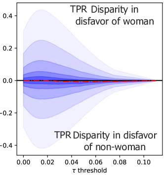
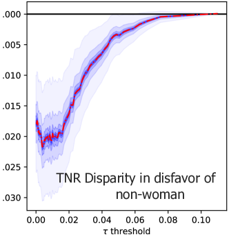
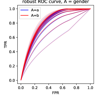
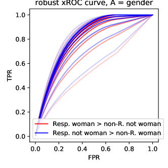
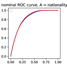
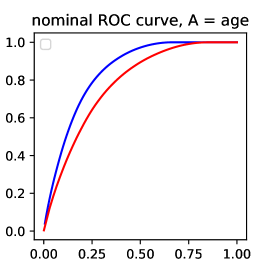
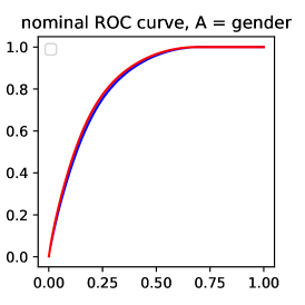
We focus on the public program vs. control arm, which enrolled about 7950 participants in total, with participants in the public program. The treatment arm, , corresponds to assignment to the public program. The original analysis suggests a small but statistically significant positive treatment effect of the public program, with an ATE of . We omit further details on the data processing to Appendix B. We consider the group indicators: nationality ( denoting French nationals vs. non-French, respectively), gender (denoting woman vs. non-woman), and age (below the age of 26 vs. above). (Figures for gender appear in Appendix B.)
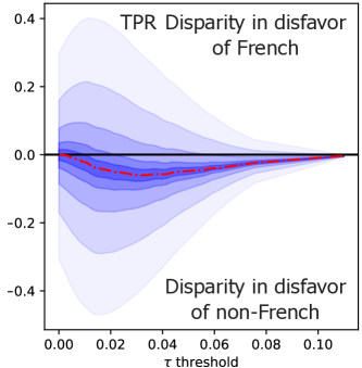
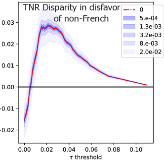
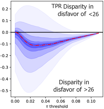
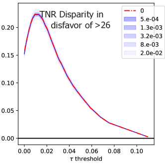
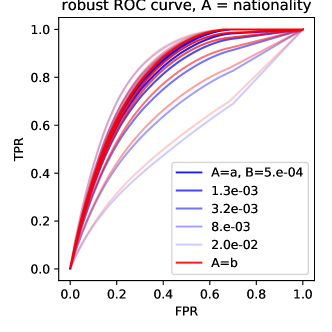
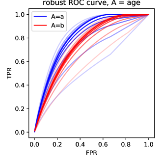
In Fig. 1, we plot the identified “disparity curves” of Eq. 5 corresponding to the maximal and minimal sensitivity bounds on TPR and TNR disparity between groups. Levels of shading correspond to different values of , with color legend at right. We learn by the Generalized Random Forests method of [53, 5] and use sample splitting, learning on half the data and using our methods to assess bounds on and other quantities with out-of-sample estimates on the other half of the data. We bootstrap over 50 sampled splits and average disparity curves to reduce sample uncertainty.
In general, the small probability of being a responder leads to increased sensitivity of TPR estimates (wide identification bands). The curves and sensitivity bounds suggest that with respect to nationality and gender, there is small or no disparity in true positive rates but the true negative rates for nationality, gender, and age may differ significantly across groups, such that non-women would have a higher chance of being bestowed job-training benefits when they are in fact not responders. However, TPR disparity by age appears to hold with as much as -0.1 difference, with older actually-responding individuals being less likely to be given job training than younger individuals. Overall, this suggests that differences in heterogeneous treatment effects across age categories could lead to significant adverse impact on older individuals.
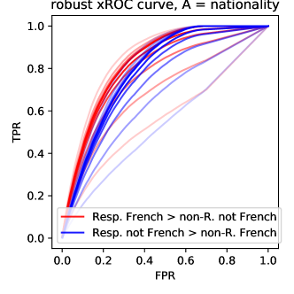
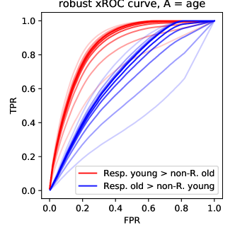
This is similarly reflected in the robust ROC, xROC curves (Fig. 2). Despite possibly small differences in ROCs, the xROCs indicate strong disparities: the sensitivity analysis suggests that the likelihood of ranking a non-responding young individual above a responding old individual (xAUC [33]) is clearly larger than the symmetric error, meaning that older individuals who benefit from the treatment may be disproportionately shut out of it as seats are instead given to non-responding younger individuals.
8 Discussion and Conclusion
We presented identification results and bounds for assessing disparate model errors of causal-effect maximizing treatment policies, which can lead disparities in access to those who stand to benefit from treatment across groups. Whether this is “unfair” would naturally rely on one’s normative assumptions. One such is “claims across outcomes,” that individuals have a claim to the public intervention if they stand to benefit, which can be understood within [1]’s axiomatic justification of fair distribution. There may also be other justice-based considerations, e.g. minimax fairness. We discuss this more extensively in Appendix C.
With the new ability to assess disparities using our results, a second natural question is whether these disparities warrant adjustment, which is easy to do given our tools combined with the approach of [25]. This question again is dependent both on one’s viewpoint and ultimately on the problem context, and we discuss it further in Appendix C. Regardless of normative viewpoints, auditing allocative disparities that would arise from the implementation of a personalized rule must be a crucial step of a responsible and convincing program evaluation. We presented fundamental identification limits to such assessments but provided sensitivity analyses that can support reliable auditing.
References
- [1] M. Adler. Well-Being and Fair Distribution.
- Angrist et al. [1996] J. D. Angrist, G. W. Imbens, and D. B. Rubin. Identification of causal effects using instrumental variables. Journal of the American statistical Association, 1996.
- Angwin et al. [2016] J. Angwin, J. Larson, S. Mattu, and L. Kirchner. Machine bias. Online., May 2016.
- Athey [2017] S. Athey. Beyond prediction: Using big data for policy problems. Science, 2017.
- Athey et al. [2019] S. Athey, J. Tibshirani, S. Wager, et al. Generalized random forests. The Annals of Statistics, 47(2):1148–1178, 2019.
- Balke and Pearl [1997] A. Balke and J. Pearl. Bounds on treatment effects from studies with imperfect compliance. Journal of the American Statistical Association, 92(439):1171–1176, 1997.
- Banerjee et al. [2015] A. Banerjee, E. Duflo, N. Goldberg, D. Karlan, R. Osei, W. Parienté, J. Shapiro, B. Thuysbaert, and C. Udry. A multifaceted program causes lasting progress for the very poor: Evidence from six countries. Science, 348(6236):1260799, 2015.
- Barabas et al. [2017] C. Barabas, K. Dinakar, J. Ito, M. Virza, and J. Zittrain. Interventions over predictions: Reframing the ethical debate for actuarial risk assessment. Proceedings of Machine Learning Research, 2017.
- Barocas and Selbst [2014] S. Barocas and A. Selbst. Big data’s disparate impact. California Law Review, 2014.
- Barocas et al. [2018] S. Barocas, M. Hardt, and A. Narayanan. Fairness and Machine Learning. fairmlbook.org, 2018. http://www.fairmlbook.org.
- Behaghel et al. [2014] L. Behaghel, B. Crépon, and M. Gurgand. Private and public provision of counseling to job seekers: Evidence from a large controlled experiment. American Economic Journal: Applied Economics, 2014.
- Behncke et al. [2007] S. Behncke, M. Frölich, and M. Lechner. Targeting labour market programmes: results from a randomized experiment. Work. Pap. 3085, IZA (Inst. Study Labor), 2007.
- Beresteanu et al. [2012] A. Beresteanu, I. Molchanov, and F. Molinari. Partial identification using random set theory. Journal of Econometrics, 166(1):17–32, 2012.
- Berger et al. [2000] M. Berger, D. A. Black, and J. A. Smith. Econometric evaluation of labour market policies, chapter EvaluatingProfiling as a Means of Allocating Government Service, pages 59–84. 2000.
- Bhattacharya and Dupas [2012] D. Bhattacharya and P. Dupas. Inferring welfare maximizing treatment assignment under budget constraints. Journal of Econometrics, 2012.
- Brown et al. [2016] C. Brown, M. Ravallion, and D. van de Walle. A poor means test? econometric targeting in africa. Policy Research Working Paper 7915: World Bank Group, Development Research Group, Human Development and Public Services Team, 2016.
- Charnes and Cooper [1962] A. Charnes and W. W. Cooper. Programming with linear fractional functionals. Naval research logistics (NRL), 9(3-4):181–186, 1962.
- Chen et al. [2018] I. Chen, F. Johansson, and D. Sontag. Why is my classifier discriminatory? In Advances in Neural Information Processing Systems 31, 2018.
- Chouldechova [2016] A. Chouldechova. Fair prediction with disparate impact: A study of bias in recidivism prediction instruments. In Proceedings of FATML, 2016.
- Corbett-Davies and Goel [2018] S. Corbett-Davies and S. Goel. The measure and mismeasure of fairness: A critical review of fair machine learning. ArXiv preprint, 2018.
- Crepon and van den Berg [2016] B. Crepon and G. J. van den Berg. Active labor market policies. Annual Review of Economics, Vol. 8:521-546, 2016.
- Davis and Heller [2017] J. M. Davis and S. B. Heller. Using causal forests to predict treatment heterogeneity: An application to summer jobs. American Economic Review: Papers and Proceedings, 107(5): 546–550, 2017.
- Dudik et al. [2014] M. Dudik, D. Erhan, J. Langford, and L. Li. Doubly robust policy evaluation and optimization. Statistical Science, 2014.
- Eubanks [2018] V. Eubanks. Automating inequality: How high-tech tools profile, police, and punish the poor. St. Martin’s Press, 2018.
- Hardt et al. [2016] M. Hardt, E. Price, N. Srebro, et al. Equality of opportunity in supervised learning. In Advances in Neural Information Processing Systems, pages 3315–3323, 2016.
- Heidari et al. [2018] H. Heidari, C. Ferrari, K. Gummadi, and A. Krause. Fairness behind a veil of ignorance: A welfare analysis for automated decision making. In Advances in Neural Information Processing Systems, pages 1265–1276, 2018.
- Hill [2011] J. L. Hill. Bayesian nonparametric modeling for causal inference. Journal of Computational and Graphical Statistics, 20(1):217–240, 2011.
- Hu and Chen [2019] L. Hu and Y. Chen. Fair classification and social welfare. arXiv preprint arXiv:1905.00147, 2019.
- Imbens and Rubin [2015] G. Imbens and D. Rubin. Causal Inference for Statistics, Social, and Biomedical Sciences. Cambridge University Press, 2015.
- Jung et al. [2018] J. Jung, R. Shroff, A. Feller, and S. Goel. Algorithmic decision making in the presence of unmeasured confounding. ArXiv, 2018.
- Kallus [2019] N. Kallus. Classifying treatment responders under causal effect monotonicity. Proceedings of International Conference on Machine Learning, 2019.
- Kallus and Zhou [2018] N. Kallus and A. Zhou. Residual unfairness in fair machine learning from prejudiced data. Forthcoming at ICML, 2018.
- Kallus and Zhou [2019] N. Kallus and A. Zhou. The fairness of risk scores beyond classification: Bipartite ranking and the xauc metric. arXiv preprint, https://arxiv.org/pdf/1902.05826.pdf, 2019.
- Kilbertus et al. [2017] N. Kilbertus, M. Rojas-Carulla, G. Parascandolo, M. Hardt, D. Janzing, and B. Schölkopf. Avoiding discrimination through causal reasoning. Advances in Neural Information Processing Systems 30, 2017, 2017.
- Kitagawa and Tetenov [2015] T. Kitagawa and A. Tetenov. Empirical welfare maximization. 2015.
- Kube and Das [2019] A. Kube and S. Das. Allocating interventions based on predicted outcomes: A case study on homelessness services. Proceedings of the AAAI Conference on Artificial Intelligence, 2019.
- Kusner et al. [2017] M. J. Kusner, J. R. Loftus, C. Russell, and R. Silva. Counterfactual fairness. NIPS, 2017.
- Lakkaraju et al. [2017] H. Lakkaraju, J. Kleinberg, J. Leskovec, J. Ludwig, and S. Mullainathan. The selective labels problem: Evaluating algorithmic predictions in the presence of unobservables. Proceedings of KKD2017, 2017.
- Liu et al. [2018] L. T. Liu, S. Dean, E. Rolf, M. Simchowitz, and M. Hardt. Delayed impact of fair machine learning. Proceedings of the 35th International Conference on Machine Learning (ICML), Stockholm, Sweden, 2018.
- Madras et al. [2019] D. Madras, E. Creager, T. Pitassi, and R. Zemel. Fairness through causal awareness: Learning latent-variable models for biased data. ACM Conference on Fairness, Accountability, and Transparency (ACM FAT*) 2019, 2019.
- Manski [2005] C. Manski. Social Choice with Partial Knoweldge of Treatment Response. The Econometric Institute Lectures, 2005.
- Manski [1997] C. F. Manski. Monotone treatment response. Econometrica: Journal of the Econometric Society, pages 1311–1334, 1997.
- Manski [2003] C. F. Manski. Partial identification of probability distributions. Springer Science & Business Media, 2003.
- McBride and Nichols [2016] L. McBride and A. Nichols. Retooling poverty targeting using out-of-sample validation and machine learning. Policy Research Working Paper 7849 (World Bank Group, Development Economics Vice Presidency Operations and Strategy Team), 2016.
- Mitchell et al. [2018] S. Mitchell, E. Potash, and S. Barocas. Prediction-based decisions and fairness: A catalogue of choices, assumptions, and definitions. arXiv, 2018.
- Mkandawire [2005] T. Mkandawire. Targeting and universalism in poverty reduction. Social Policy and Development, 2005.
- Rice [2013] E. Rice. The tay triage tool: A tool to identify homeless transition age youth most in need of permanent supportive housing. 2013.
- Rockafellar [2015] R. T. Rockafellar. Convex analysis. Princeton university press, 2015.
- Rubin [1980] D. B. Rubin. Comments on “randomization analysis of experimental data: The fisher randomization test comment”. Journal of the American Statistical Association, 75(371):591–593, 1980.
- Shalit et al. [2017] U. Shalit, F. Johansson, and D. Sontag. Estimating individual treatment effect: generalization bounds and algorithms. Proceedings of the 34th International Conference on Machine Learning, 2017.
- Shroff [2017] R. Shroff. Predictive analytics for city agencies: Lessons from children’s services. Big data, 5(3):189–196, 2017.
- Wager and Athey [2017a] S. Wager and S. Athey. Efficient policy learning. 2017a.
- Wager and Athey [2017b] S. Wager and S. Athey. Estimation and inference of heterogeneous treatment effects using random forests. Journal of the American Statistical Association, (just-accepted), 2017b.
Appendix A Omitted proofs
Proof of Proposition 1.
To prove this we exhibit a simple example satisfying ignorability where both and differences therein varies while the joint distribution of does not.
Let , , , . To specify a joint distribution of that satisfies ignorable treatment, it only remains to specify .
Note that in this case
The result follows by noting that where the corresponding joint distribution of is completely specified by , while could vary as long as these sums are neither 0 nor 1. Since we can vary this independently across values of , differences are not identifiable either. ∎
Proof of Proposition 2.
where the first equality holds by Bayes’ rule, the second by iterating expectations on and Assumption 1, and the third by unconfoundedness and consistency of potential outcomes. The proof for identification of is identical for the quantity . ∎
Proof of Proposition 3.
Proof of Proposition 4.
The support function evaluated at is:
We apply the Charnes-Cooper transformation [17]with the bijection . The denominator of the second term under this bijection is equivalently
such that we can rewrite the second term as
and the objective function overall as:
The new constraint set (including the constraint yielding the definition of ) is:
∎
Proof of Proposition 5.
We first consider the case of maximizing or minimizing the TPR.
We leverage the invariance in the objective function under the surjection on to its marginal expectation over a partition.
Therefore we can reparametrize the program as optimizing over coefficients of the optimal solution, . Define the fractional objective
First note that without loss of generality that when maximizing, we can set since this decreases the objective regardless of the value of . We can consider the constrained problem where . Then we have the first and second derivatives,
By inspection, since we have that so the function is convex. So when maximizing on the constraints for , it attains optimal value at the boundary (since is increasing). When minimizing, note that the derivative is not vanishing anywhere on the constraint set so it suffices to check the endpoints, where the minimum is achieved at .
We now consider the case of minimizing or maximizing the TNR.
Now consider a generic which represents the TNR sensitivity bound with , and the constants
Without loss of generality we know that we can set to its upper bound when maximizing as we are only increasing the objective value; then . We verify that the second derivative is negative, so that the function is concave:
Checking the sign of the numerator simplifies to checking the sign of
which is negative. The denominator is lower bounded by which is always positive: therefore the problem is concave. The first derivative is negative on the domain; therefore the maximum is achieved at . Therefore, when maximizing, .
For minimizing the TPR, we take a similar approach: analogously, we can set to its lower bound without loss of generality. Following the same analysis, the function is still concave since and decreasing with nonzero first-derivative; so the minimum is achieved at .
∎
Appendix B Behaghel et al. Job Training
We processed the data using replication files available with the AEJ: Applied Economics journal electronic supplement. For the sake of simplicity, we analyze the trial as if it were a randomized controlled trial (without accounting for noncompliance or different randomization probabilities that differ by region). Thus, we consider intention-to-treat effects (as intention to treat is ultimately the policy lever available). We further restricted some covariates, omitting some where personalized allocation based on these covariates seemed unilkely for fairness reasons. The covariates we retain include: length of previous employment, salary, education level, reason for unemployment, region, years of experience at previous job, statistical risk level, job search type (full-time or non-full time), wage target, time of first unemployment spell, job type, and number of children.
An interacted linear model indicates potential heterogeneity of treatment effect with significance on college education, economic layoff, those seeking work due to fixed term contracts or those with previous layoffs.
Appendix C Substantive Discussion: Fairness vs. Justice
We first caveat our use of “disparate impact”: while our selection of protected attibutes parallels choices of protected attributes that appear elsewhere in the literature on fair machine learning, for the case of interventions, there may not be precedent from discrimination case law, nonetheless assessing fairness with respect to these social groups may be of concern. We view disparate impact in this domain as assessing fairness of outcome rates under a personalization model.
Should true positive rates be adjusted for?
Our presentation of an identification strategy of fairness metrics for allocating interventions with unknown causal effects begs the question: should disparities in TPR and FNR be adjusted for in the interventional welfare setting? Is responder-accuracy parity a meaningful prescriptive notion of fairness?
One critique of outcome-conditional fair classification metrics recognizes the dependence of false positive rates on the underlying base rate, , [20, 19]. The equivalent situation occurs when the within-group ATE varies by the protected attribute, e.g. differs.
Ultimately, external domain knowledge is required to adjudicate whether group-wide disparities in ATE should be adjusted for, or to decide which normative notion of distributive justice or fairness is appropriate. For example, consider the case of job training. From an economic perspective, multiple mechanisms could explain heterogeneity in CATE by race. Active labor market programs (see [21]) may be less effective for one group vs. another group due to the presence of labor-market discrimination. Alternatively, they could be less effective due to correlation of group status and efficacy that is mediated by occupation choice: one group may be more interested in labor markets where the primary benefits of job search counseling, in reducing search frictions, are not barriers to employment in the first place relative to other factors such as skills gaps. Intuitively, the former mechanism of ATE variation by group reflects a notion of “disparity” which remains problematic, while the latter may seem to reflect an unproblematic causal mechanism. While mediation analysis and fairness defined in terms of path-specific effects could further decompose the treatment effect along these stated mechanisms, in policy settings, collecting all of the relevant information can be burdensome, and deciding on a causal graph can be difficult.
Claims Across Outcomes We first outline different frameworks for thinking about fairness/equity of algorithms and interventions. Analogous to the proposals arising from metrics proposed in fairness in machine learning, one might view the decision-maker’s concern to be of ensuring accuracy parity, that the decisions meted out are overall beneficial to individual. We view a theory of fairness that assesses disparities in outcome-conditional error rates in the context of a theory of normative claims arising from “claims across outcomes”. [1] develops a “claims across outcomes” framework of fairness and social welfare, in the context of an overall welfarist theory of justice.
On the one hand, fair classification from the point of view of assessing or equalizing TPR or TNR disparities may be interpreted in a claims context as: for an individual with “true outcome” and covariates , an individual with the true label as having a comparative claim for , if the predictor is an allocation tool. We can map the setting of personalized interventions to the “claims across outcomes” setting: the potential outcomes framework posits for each individual the random variables of outcomes . In the responder setting, the true label is responder status . However, since these are jointly unobservable, in situations where heterogeneous treatment effects are plausible, the best guess is an individual-level treatment effect conditional on covariates, . In this interventional setting, one can think of individuals having claims in favor of favorable outcomes, e.g. a claim in favor of if .
For the case of interventions, classification decisions are allocative of real interventions, and we argue that implicitly, the consideration of social welfare (balancing efficiency and program costs) is an important factor in the original design of social programs or personalized interventions. This is in sharp contrast to the literature on fair classification which considers settings such as lending in finance, or risk prediction in the criminal justice system, where overriding concerns are primarily those of vendor utility.
On the other side of the spectrum, we can recall axiomatically justified social welfare functions that apply to the case of deterministic resource allocation, where outcomes are generally known. A decision-maker might also be concerned with equity considerations, adopting a min-max welfare criterion, appealing to Rawlsian justice frameworks. Another approach is simply assessing the population cardinal welfare of the allocation, e.g. the policy value or a social-welfare transformation thereof, . The literature on policy learning addresses welfare functionals that are linear functionals of potential outcomes, see [35]. Cardinal welfare constraints such as those studied in [26] can be applied with an imputed CATE function.
Comparison to other work on fair classification and welfare.
[39] study the implications of classifier-based decisions, as well as proposals for statistical parity, on group welfare. Their work addresses selection rules that have known marginal impacts by group. [28] studies the welfare weights implied by classification parity metrics and shows that enforcing classification parity metrics are not Pareto-improving. Rather than studying the welfare implications of classification parity, we are concerned with assessing non-identifiable model errors in the causal-effect personalized intervention setting. Since in the personalized intervention setting, welfare is a primary objective for the Planner (e.g. social services, or social protection more broadly), modulo cost considerations, combining the distributional information from identification of classification errors with other social welfare objectives is of possible interest.
We next aim to provide concrete examples of discussions regarding the distributional impacts of interventions, in order to provide additional context on different contexts wherein different notions of “fairness” from the fairness in machine learning literature map onto welfare or justice concerns, as stated in discussions on interventional outcomes.
Lexicographic fairness or maximin (Rawlsian) fairness.
In a large multi-site graduation trial on testing an intensive, composite intervention targeted at the "ultra-poor", which comprised wraparound services including coaching and revenue-generating resources, still the poorest seemed to benefit least from the intervention in terms of sustained revenue [7]. In this setting, concerns about maximin fairness (Rawlsian justice) might override considerations of efficiency insofar as one might be willing to invest resources to help the worst-off on humanitarian grounds.
Universalism.
Criticisms of targeted policies in general note practical difficulties introduced by imposing and enforcing eligibility guidelines. [46]. Although discussion of resource constraints may be used to justify a targeting scheme, critics of targeting argue that the most efficient targeting is not as welfare-improving as simply advocating for greater resources [24].
Additional distributional preferences on with respect to equitable or redistributive aims of the policy.
[14] consider profiling based on covariates as a means of allocating government services, in the example of allocating predicting unemployment duration to allocate reemployment services. They outline competing equity vs. efficiency concerns, in the case that unemployment duration is correlated with treatment efficacy (e.g efficacy of reemployment services), and conclude that “ tradeoffs between alternative social goals in designing profiling systems are likely to be empirically important… the form and extent of these tradeoffs may depend on empirical relationships between the impacts of the program being allocated and the equity-related characteristics of potential participants." While outcome-conditional true positive rates or true negative rates compare model performance across binary protected attributes, program designers may remain concerned regarding the distribution of benefits. [carneiro2002removing] consider “removing the veil of ignorance” under the simplifying of constant treatment response to consider distributional (quantile) treatment effects, as a relaxation of the anonymity axiom of cardinal social welfare. Distributional preferences are relevant when program designers are concerned about model performance at finer-grained levels than discrete protected attribute.