Extrapolation Methods for fixed-point Multilinear PageRank computations

Abstract

Nonnegative tensors arise very naturally in many applications that involve large and complex data flows. Due to the relatively small requirement in terms of memory storage and number of operations per step, the (shifted) higher-order power method is one of the most commonly used technique for the computation of positive $Z$-eigenvectors of this type of tensors. However, unlike the matrix case, the method may fail to converge even for irreducible tensors. Moreover, when it converges, its convergence rate can be very slow. These two drawbacks often make the computation of the eigenvectors demanding or unfeasible for large problems. In this work we consider a particular class of nonnegative tensors associated to the multilinear PageRank modification of higher-order Markov chains. Based on the simplified topological $\varepsilon$-algorithm in its restarted form, we introduce an extrapolation-based acceleration of power method type algorithms, namely the shifted fixed-point method and the inner-outer method. The accelerated methods show remarkably better performance, with faster convergence rates and reduced overall computational time. Extensive numerical experiments on synthetic and real-world datasets demonstrate the advantages of the introduced extrapolation techniques.

Keywords— tensor, multilinear PageRank, graphs, higher-order Markov chains, extrapolation methods, acceleration of convergence, fixed-point, Spacey Random Surfer, higher-order power method

1 Introduction

A higher-order Markov chain with memory of length $m-1$ is a stochastic process $\{S_{t}\}_{t=0}^{\infty}$ over a finite state space $V=\{1,\dots,n\}$ where the conditional probability distribution of the next state in the process depends only on the last $m-1$ states. As for standard chains with memory of length 1, a higher-order Markov chain with a memory of length $m-1$ can be represented by the $m$-order transition tensor

$$p_{{i_{1}},{i_{2}\dots,i_{m}}}:=\mathbb{P}(S_{t}={i_{1}}|S_{t-1}={i_{2}},\cdots,S_{t-(m-1)}={i_{m}}),\qquad\forall\;t\,.$$

Note that by definition we obtain $p_{{i_{1}},{i_{2}\dots,i_{m}}}\geq 0$ and $\sum_{{i_{1}}=1}^{n}p_{{i_{1}},{i_{2}\dots,i_{m}}}=1$ for all $({i_{2},\dots,i_{m}})$. The stationary distribution $s_{i_{1},\dots,i_{m-1}}$ of the chain is thus given by

$$\sum_{i_{m}=1}^{n}p_{i_{1},\dots,i_{m}}s_{i_{2},\dots,i_{m}}=s_{i_{1},\dots,i_{m-1}}\,.$$ (1)

As on the one hand, a longer memory has the advantage of allowing more accurate models and thus may offer additional predictive value, on the other hand, computing a stationary distribution for a Markov chain with memory length $m-1$ requires the computation of $n^{m-1}$ parameters and thus the memory requirement and the computational cost to treat the stationary distribution (1) become extremely demanding already for moderate values of $m$ and $n$ [57].

In this work we are particularly interested in PageRank-type chains. In the standard single-order setting, given a random walk on a directed graph with $n$ nodes, the PageRank modification builds a new Markov chain that has always a unique stationary distribution. Since its introduction [46], the analysis of the PageRank random walk and its stationary distribution has given rise to a wide literature, with applications going further beyond the initial treatment of the web hyperlinks network [30]. In particular, the very large size of typical problems where the PageRank is applied has led to the development of several algorithms for its numerical treatment, ranging from specialized versions of the power, Jacobi and Richardson methods [4, 21, 55, 23, 35], to algebraic and Krylov-type methods [33, 48]. In particular, the use of extrapolation strategies has shown to be very effective in this context [9, 10, 16, 36].

Recently, the PageRank idea has been extended to higher-order Markov chains [32]. However, due to the exponential complexity required by the higher-order setting, the authors further introduce a computationally tractable approximation of the true higher-order PageRank distribution, called multilinear PageRank. From the algebraic point of view, the multilinear PageRank seeks a rank-one stationary distribution of the higher-order chain, i.e., the joint probability $s_{i_{1},\dots,i_{m-1}}$ solution of (1) is replaced by a rank-one tensor $s_{i_{1}}s_{i_{2}}\cdots s_{i_{m-1}}$. This formulation dramatically reduces the dimension of the solution set from $n^{m-1}$ to $n$. Moreover, it has been proved in [41] that, under the assumption $s_{i_{1},\dots,i_{m-1}}=s_{i_{1}}s_{i_{2}}\cdots s_{i_{m-1}}$, the solution of (1) coincides with a $Z$-eigenvector of the transition tensor, given by

$$\sum_{i_{2},\dots,i_{m}}p_{i_{1},\dots,i_{m}}s_{i_{2}}\cdots s_{i_{m}}=s_{i_{1}},\qquad\forall i_{1}=1,\dots,n\,.$$ (2)

Motivated by the success that extrapolation methods have had in the computation of the single-order PageRank, in this work we propose and investigate the use of extrapolation methods, based on Shanks transformations [15, 49], for the particular setting of tensor $Z$-eigenpairs problems arising from the analysis of the multilinear PageRank. More precisely, after a short survey on results about existence and uniqueness of the solution and on the state-of-the-art fixed-point computational methods for the multilinear PageRank vector, we will show how its computation can be considerably sped-up using extrapolation techniques. In particular, we will show that the sequences generated by the two fixed-point-type techniques Shifted Higher-Order Power Method [32, 38] and Inner-Outer Method [32], are strongly accelerated using the The Simplified Topological $\varepsilon$-Algorithm (STEA) [11, 13] in the restarted form. Alongside fixed-point methods, techniques based on the Newton’s method have been proposed for instance in [32, 42]. The results presented in this work show that the use of the extrapolation framework based on the Simplified Topological $\varepsilon$-Algorithm allows us to improve the efficiency and the robustness of fixed-point iterations without resorting on the Newton’s framework which requires, for large scale problems, a severe computational cost.

The use of simplified topological extrapolation techniques for this type of problem is, to our knowledge, a useful and effective novelty. For example, it gives a positive answer to the question (quoting from [38]) Can the convergence rate of the current SS-HOPM method be accelerated? The introduction of the extrapolation framework and the acceleration techniques here considered not only produce a relevant speed-up but also enhance the robustness of the method without modifying the overall computational cost of the underlying iterative procedure (see Section 3.1). Moreover, as the multilinear PageRank is an instance of the many eigenvector problems that correspond to nonnegative tensors [29], the results proposed here can be transferred to a variety of data analysis applications where nonnegative tensors and their spectra play an important role. Examples, involving nonnegative tensors in general and the multilinear PageRank in particular, include ranking of nodes in multilayer networks [43, 53, 1], data clustering [2, 57], hypergraph matching [19, 45], computer vision [50] and image reconstruction [51]. Although much has been done in recent years, much is still unknown for tensor eigenpairs, including the development of fast algorithms for their computation. To this end, higher-order and nonlinear versions of the classic power method have been proposed to address the computation of different types of tensors eigenpairs (see e.g. [26, 28, 29, 37, 38, 44]) and, due to the large size of typical problems, enhancing the efficiency and robustness of these methods is of utmost importance.

The reminder of this paper is organized as follows: in Section 2 we introduce and review all the necessary theory concerning the multilinear PageRank problem and related computational techniques and we analyze the existence and uniqueness issue of the multilinear Pagerank problem. In Section 3, after introducing and reviewing the topological extrapolation framework, we describe our proposed simplified topological extrapolation method with restart and detail how we apply it to the specific multilinear PageRank case; finally, in Section 4 we present extensive numerical results on synthetic and real-world datasets that showcase the effectiveness and the advantages of our approach.

2 Multilinear PageRank

2.1 Notation

We say that $\mathcal{A}$ is a real cubical tensor of order $m$ and dimension $n$ if $\mathcal{A}$ is a multi-dimensional array with real entries such that

$$\mathcal{A}=(a_{i_{1},\dots,i_{m}})\quad\text{with}\quad i_{1},\dots,i_{m}\in\{1,\dots,n\}\,.$$

Given a vector ${\mathbf{s}}\in{\mathbb{R}}^{n}$ we denote by $\mathcal{A}{\mathbf{s}}^{m-1}\in{\mathbb{R}}^{n}$ the vector with entries

$$(\mathcal{A}{\mathbf{s}}^{m-1})_{i_{1}}=\sum_{i_{2},\dots,i_{m}=1}^{n}a_{i_{1},i_{2},\dots,i_{m}}s_{i_{2}}\dots s_{i_{m}},\qquad i_{1}=1,\dots,n$$

A vector ${\mathbf{s}}=(s_{i})\in{\mathbb{R}}^{n}$ is said to be stochastic or, equivalently, a probability distribution, if $s_{i}\geq 0$ for all $i=1,\dots,n$ and $\sum_{i}s_{i}=1$. Similarly, a real cubical tensor $\mathcal{A}$ is said to be stochastic if its entries are nonnegative numbers and the entries on the first mode of $\mathcal{A}$ sum up to one, namely

$$a_{i_{1},\dots,i_{m}}\geq 0,\quad\forall i_{1},\dots,i_{m}\in\{1,\dots,n\}\qquad\text{and}\qquad\sum_{i_{1}=1}^{n}a_{i_{1},\dots,i_{m}}=1\,.$$

Unlike the matrix case, a number of different types of tensor eigenvectors can be defined, see for instance [29] and the references therein.

Here we are concerned with $Z$-eigenvectors: a number $\lambda\in\mathbb{C}$ is an $E$-eigenvalue of ${\mathcal{A}}$ with $E$-eigenvector ${\mathbf{s}}\in\mathbb{C}^{n}$ if it holds

$${\mathcal{A}}{\mathbf{s}}^{m-1}=\lambda\,{\mathbf{s}}\qquad\text{and}\qquad\|{\mathbf{s}}\|_{1}=\sum_{i=1}^{n}|s_{i}|=1\,.$$ (3)

A real $E$-eigenvector ${\mathbf{s}}\in\mathbb{R}^{n}$ is called $Z$-eigenvector and the corresponding $\lambda$ a $Z$-eigenvalue. We point out that, although the normalization constraint on ${\mathbf{s}}$ in the definition (3) is more commonly given in terms of the Euclidean norm $\|\cdot\|_{2}$, we require here the $1$-norm for the sake of convenience. In fact, this is the choice that is more natural when dealing with stochastic tensors, as in that case it easy to see that the only $Z$-eigenvalue $\lambda$ of a nonnegative $Z$-eigenvector is $\lambda=1$. For reference, we also point out that ${\mathbf{s}}$, solution of (3), is sometimes called $Z_{1}$-eigenvector to underline the choice of the one norm (see e.g. [17]). We avoid this additional notation, for the sake of simplicity.

Finally, as for nonnegative matrices, the concept of (nonnegative) irreducible tensor is important in order to show existence and uniqueness of nonnegative tensor eigenvectors. Again, unlike the matrix case, the concept of irreducible tensor is not “universal” but strongly depends on the structure of ${\mathcal{A}}$ and on the eigenvector problem one is interested in (see [29] for a thorough discussion on the topic). In this work we focus on the following notion of irreducible cubical tensors, originally proposed in [18]

Definition 1.

A $n$-dimensional order-$m$ nonnegative cubical tensor ${\mathcal{A}}$ is called reducible if there exists a set of indices $I\subseteq V=\{1,\dots,n\}$, $I\neq\emptyset$, $I\neq V$, such that

$$a_{i_{1},i_{2},\dots,i_{m}}=0,\qquad\forall i_{1}\in I,\qquad\forall i_{2},\dots,i_{m}\notin I\,.$$

The tensor ${\mathcal{A}}$ is irreducible if it is not reducible.

2.2 Background

Let $\Omega\subseteq{\mathbb{R}}^{n}$ be the set of all stochastic vectors

$$\Omega:=\Big{\{}{\mathbf{s}}\in\mathbb{R}^{n}\;:\;\sum_{i=1}^{n}s_{i}=1,\,{s}_{i}\geq 0,i=1,\dots,n\Big{\}},$$

and let $\Omega_{+}\subseteq\Omega$ be the set of entry-wise positive stochastic vectors.

The multilinear PageRank model proposed in [32] seeks a fixed-point solution in $\Omega$ of the following nonlinear map:

$$f({\mathbf{s}})=\alpha{\mathcal{P}}{\mathbf{s}}^{m-1}+(1-\alpha){\mathbf{v}},$$ (4)

being ${\mathcal{P}}=(p_{i_{1},\dots,i_{m}})$ a stochastic tensor ($\sum_{i_{1}}p_{i_{1},\dots,i_{m}}=1$) and ${\mathbf{v}}\in\Omega_{+}$ the so-called “teleportation vector”. It is worth point out that a solution of (4) is a stationary distribution of a stochastic process called “The Spacey Random Surfer” [3] which is an interesting vertex-reinforced Markov process that uses a combination of an aggregated history and the current state.

The map (4) is reminiscent of the standard single-order PageRank model. In that case, given the transition matrix $P=(p_{ij})$, $\sum_{i}p_{ij}=1$, of a random walk on a graph with $n$ nodes $V=\{1,\dots,n\}$ and given ${\mathbf{v}}=(v_{1},\dots,v_{n})\in\Omega_{+}$, one seeks to compute a positive eigenvector of the PageRank transition matrix

$$P_{\scalebox{0.5}{{PR}}}=\alpha P+(1-\alpha){\mathbf{v}}{\mathbf{e}}^{T},$$ (5)

where ${\mathbf{e}}$ is the vector of all ones. Such PageRank transition matrix $P_{\scalebox{0.5}{{PR}}}$ models a new random walk where one takes a step according to the initial Markov chain with probability $\alpha$, and with probability $1-\alpha$ randomly jumps to node $i$ according to the fixed teleportation probability $v_{i}>0$. Note that, as ${\mathbf{v}}\in\Omega_{+}$, for any $0\leq\alpha<1$ the PageRank matrix $P_{\scalebox{0.5}{{PR}}}$ is irreducible and thus, by the Perron-Frobenius theorem, there exists a unique positive eigenvector ${\mathbf{s}}\in\Omega_{+}$ such that $P_{\scalebox{0.5}{{PR}}}{\mathbf{s}}={\mathbf{s}}$ [4, 54, 56]. The analogy with (4) essentially follows by (3). In fact, it is not difficult to observe that the proposed multilinear PageRank, solution of (4), coincides with a nonnegative $Z$-eigenvector of the PageRank transition tensor $\mathcal{P}_{\scalebox{0.5}{{PR}}}$, i.e. it solves (3).

More precisely, given a stochastic tensor ${\mathcal{P}}$ describing the transition probabilities of a higher-order random walk on a graph with $n$ nodes, consider the following PageRank transition tensor

$${\mathcal{P}}_{\scalebox{0.5}{{PR}}}:=\alpha{\mathcal{P}}+(1-\alpha){\mathcal{V}},$$ (6)

where, given the teleportation vector ${\mathbf{v}}\in\Omega_{+}$ and the all-ones vector ${\mathbf{e}}$, ${\mathcal{V}}$ is the rank-one positive tensor ${\mathcal{V}}={\mathbf{v}}\otimes{\mathbf{e}}\otimes\dots\otimes{\mathbf{e}}$, with entries ${\mathcal{V}}_{i_{1},\dots,i_{m}}=v_{i_{1}}$. Now, for any ${\mathbf{s}}\in\Omega$ we have ${\mathcal{V}}{\mathbf{s}}^{m-1}=({\mathbf{v}}\otimes{\mathbf{e}}\otimes\dots\otimes{\mathbf{e}}){\mathbf{s}}^{m-1}=({\mathbf{e}}^{T}{\mathbf{s}})^{m-1}{\mathbf{v}}={\mathbf{v}}$ and thus it holds

$${\mathcal{P}}_{\scalebox{0.5}{{PR}}}{{\mathbf{s}}}^{m-1}=\alpha{\mathcal{P}}{{\mathbf{s}}}^{m-1}+(1-\alpha){\mathcal{V}}{{\mathbf{s}}}^{m-1}=\alpha{\mathcal{P}}{{\mathbf{s}}}^{m-1}+(1-\alpha){\mathbf{v}},$$ (7)

showing that ${\mathbf{s}}\in\Omega$ is a fixed-point of (4) if and only if ${\mathcal{P}}_{\scalebox{0.5}{{PR}}}{\mathbf{s}}^{m-1}={\mathbf{s}}$.

This tensor eigenvector formulation unveils an elegant conceptual analogy with the matrix case which, however, comes with several fundamental differences. Tensor eigenvectors can be defined in a number of different ways, including the $Z$-eigenvector formulation we are concerned with in this work. The Perron-Frobenius theory for nonnegative tensors and the numerous corresponding spectral problems is still an active field of research (see for instance [29] and the references therein). Several drawbacks arise due the nonlinearity introduced by the additional dimensions and the Perron-Frobenius theorems developed so far show many crucial differences with respect to the matrix case. For example, unlike the stochastic matrix case, the irreducibility of the stochastic tensor ${\mathcal{P}}_{\scalebox{0.5}{{PR}}}$ is not enough to ensure the uniqueness of nonnegative fixed points of (4), whereas existence is guaranteed in both cases by the Brower’s fixed-point theorem [20]. This is shown by the following example, borrowed from [47] (see [17] for another example):

Example[47] Consider the stochastic tensor

$$\begin{split}&\mathcal{P}(:,:,1)=\begin{bmatrix}\frac{232873}{319300}&\frac{7}{10}&\frac{3}{10}\\ \\ \frac{27}{100}&\frac{470171}{2\times 814300}&\frac{378421}{2\times 407150}\\ \\ \frac{54}{79825}&\frac{18409}{2\times 814300}&\frac{191589}{2\times 407150}\end{bmatrix},\quad\mathcal{P}(:,:,2)=\begin{bmatrix}\frac{7}{10}&\frac{4717}{10300}&\frac{1}{100}\\ \\ \frac{470171}{2\times 814300}&\frac{1}{2}&\frac{158157}{2\times 814300}\\ \\ \frac{18409}{2\times 814300}&\frac{433}{10300}&\frac{1454157}{2\times 814300}\end{bmatrix},\\ &\mathcal{P}(:,:,3)=\begin{bmatrix}\frac{3}{10}&\frac{1}{100}&\frac{207}{63860}\\ \\ \frac{378421}{2\times 407150}&\frac{158157}{2\times 814300}&\frac{3}{20}\\ \\ \frac{191589}{2\times 407150}&\frac{1454157}{2\times 814300}&\frac{27037}{31930}\end{bmatrix}.\end{split}$$

Note that such tensor is entry-wise positive, thus it is irreducible. However, it is such that $\mathcal{P}\mathbf{x}_{i}^{2}=\mathbf{x}_{i}$ for $i=1,2,3$, where $\mathbf{x}_{1}=[0.1,0.2,0.7]^{T}$, $\mathbf{x}_{2}=[0.4,0.3,0.3]^{T}$ and $\mathbf{x}_{3}=[0.59,0.31,0.1]^{T}$.

More precisely, for the case of $Z$-eigenvector and, specifically, for the multilinear PageRank tensor $\mathcal{P}_{\scalebox{0.5}{{PR}}}$, we recall the following two existence and uniqueness results.

Theorem 1 ([41]).

If ${\mathcal{A}}$ is a real $n$ dimensional stochastic tensor of order $m$, then there exists a nonnegative vector ${\mathbf{s}}\in\Omega$ such that ${\mathcal{A}}{{\mathbf{s}}}^{m-1}={{\mathbf{s}}}$. In particular, if ${\mathcal{A}}$ is irreducible, then ${{\mathbf{s}}}$ is positive.

Observe that if ${\mathbf{v}}\in\Omega_{+}$, then ${\mathcal{P}}_{\scalebox{0.5}{{PR}}}$ is stochastic and irreducible. In fact,

$$\sum_{i_{1}=1}^{n}({\mathcal{P}}_{\scalebox{0.5}{{PR}}})_{i_{1},\dots,i_{m}}=\alpha\sum_{i_{1}=1}^{n}p_{i_{1},\dots,i_{m}}+(1-\alpha)\sum_{i_{1}=1}^{n}v_{i_{1}}=1$$

and, for any $I\subset V=\{1,\dots,n\}$, we have

$$({\mathcal{P}}_{\scalebox{0.5}{{PR}}})_{i_{1},\dots,i_{m}}\geq(1-\alpha)v_{i_{1}}>0$$

for all $i_{1}\in I$ and $i_{2},\dots,i_{m}\notin I$. Hence, Theorem 1 ensures existence of at least one solution of (4), namely there exists ${\mathbf{s}}\in\Omega$ such that ${\mathcal{P}}_{\scalebox{0.5}{{PR}}}{\mathbf{s}}^{m-1}={\mathbf{s}}$ and this solution is positive if ${\mathbf{v}}\in\Omega_{+}$. Uniqueness, however, is guaranteed only under somewhat restrictive conditions on $\alpha$. For example, the following result holds (see [25] for more information on uniqueness of fixed-point for generic stochastic tensors and [40] for the specific case of the multilinear PageRank):

Theorem 2 ([32]).

Let ${\mathcal{P}}$ be a $n$ dimensional stochastic tensor of order $m$ and let ${\mathbf{v}}$ be a nonnegative teleportation vector. Then the multilinear PageRank equation

$${\mathcal{P}}_{\scalebox{0.5}{{PR}}}{\mathbf{s}}^{m-1}=\alpha{\mathcal{P}}{{\mathbf{s}}}^{m-1}+(1-\alpha){\mathbf{v}}={\mathbf{s}}$$

has a unique solution if $\alpha<(m-1)^{-1}$.

As in the single-order case, we are particularly interested in the case $\alpha\approx 1$. This is because one of the main reasons for introducing the rank-one perturbation $(1-\alpha)\mathcal{V}$ is exactly to ensure irreducibility of ${\mathcal{P}}_{\scalebox{0.5}{{PR}}}$ (and thus existence of a positive solution, in this case). However, since we are ideally interested in the stationary solution of the original higher-order chain, the most interesting and relevant problem settings require a very small random surfing perturbation $(1-\alpha)\mathcal{V}$. In fact, the PageRank solution largely depends on the parameter $\alpha$, as the following bound shows (see also [25])

Proposition 1.

Consider ${\mathcal{P}}_{\scalebox{0.5}{{PR}}}(\alpha):=\alpha{\mathcal{P}}+(1-\alpha){\mathcal{V}}$, ${\mathcal{P}}_{\scalebox{0.5}{{PR}}}(\beta):=\beta{\mathcal{P}}+(1-\beta){\mathcal{V}}$ with $\alpha,\beta\in(0,1)$, and let ${\mathbf{s}}_{\alpha}$ and ${\mathbf{s}}_{\beta}$ be corresponding PageRank solutions. Then, if $0<\alpha<1/(m-1)$, we have

$$\|{\mathbf{s}}_{\alpha}-{\mathbf{s}}_{\beta}\|_{1}\leq\frac{2\,|\beta-\alpha|}{1-\alpha(m-1)}.$$

Proof.

By adding and subtracting $\alpha{\mathcal{P}}{\mathbf{s}}_{\beta}^{m-1}$ from $\|{\mathbf{s}}_{\alpha}-{\mathbf{s}}_{\beta}\|_{1}=\|{\mathcal{P}}_{\scalebox{0.5}{{PR}}}(\alpha){\mathbf{s}}_{\alpha}^{m-1}-{\mathcal{P}}_{\scalebox{0.5}{{PR}}}(\beta){\mathbf{s}}_{\beta}^{m-1}\|_{1}$ and using the inequality $\|{\mathcal{P}}\|_{1}\leq 1$ we obtain

$$\begin{aligned} \|{\mathbf{s}}_{\alpha}-{\mathbf{s}}_{\beta}\|_{1}&=\|\alpha{\mathcal{P}}{\mathbf{s}}_{\alpha}^{m-1}-\beta{\mathcal{P}}{\mathbf{s}}_{\beta}^{m-1}+(\beta-\alpha){\mathbf{v}}+\alpha{\mathcal{P}}{\mathbf{s}}_{\beta}^{m-1}-\alpha{\mathcal{P}}{\mathbf{s}}_{\beta}^{m-1}\|\\ &\leq\alpha(m-1)\|{\mathcal{P}}\|_{1}\|{\mathbf{s}}_{\alpha}-{\mathbf{s}}_{\beta}\|_{1}+|\alpha-\beta|\,\|{\mathcal{P}}\|_{1}\|{\mathbf{s}}_{\beta}\|_{1}+|\alpha-\beta|\,\|{\mathbf{v}}\|_{1}\\ &\leq\alpha(m-1)\|{\mathbf{s}}_{\alpha}-{\mathbf{s}}_{\beta}\|_{1}+|\alpha-\beta|\,\|{\mathbf{s}}_{\beta}\|_{1}+|\alpha-\beta|\,\|{\mathbf{v}}\|_{1}\,.\end{aligned}$$

Thus, as $\|{\mathbf{s}}_{\beta}\|_{1}=\|{\mathbf{v}}\|_{1}=1$, we obtain

$$\big{(}1-\alpha(m-1)\big{)}\|{\mathbf{s}}_{\alpha}-{\mathbf{s}}_{\beta}\|_{1}\leq 2|\alpha-\beta|$$

and the thesis follows by rearranging terms. ∎

On the other hand, as observed in [32] and as highlighted by the numerical experiments we will present in Section 4, solving the multilinear PageRank problem as the fixed point of $f$ defined in (4) becomes more difficult when $\alpha$ gets closer to one. This is largely due to the fact that the contractivity of the map $f$ decreases when $\alpha$ increases. This phenomenon is shown for example in [27], where the contractivity of the map ${\mathbf{s}}\mapsto{\mathcal{A}}{\mathbf{s}}^{m-1}$ is analyzed in terms of the entries of ${\mathcal{A}}$, and thus of $\alpha$ in our setting ${\mathcal{A}}={\mathcal{P}}_{\scalebox{0.5}{{PR}}}$. Similar contractivity conditions on $\alpha$ are also proved in [32, 40], for the specific PageRank case.

In the following section we review two fixed-point iterative techniques for computing a solution of (4). Then, in Section 3, we introduce our new acceleration framework based on the Simplified Topological $\varepsilon$-algorithm.

2.3 Power methods for the multilinear PageRank

Due to their simplicity of implementation and their cheap storage requirements, power method-type iterations are typically the preferred choice for large scale problems. However, in the higher-order setting, their convergence behavior may be particularly unfavorable. In this section we review the shifted higher-order power method (an ad-hoc version of the SS-HOPM method originally introduced in [38]) and the inner-outer method [32] for the computation of the multilinear PageRank vector and their convergence properties. We then introduce a restarted extrapolation framework, based on the simplified topological $\varepsilon$-algorithm [11, 13], that allows to strongly improve the convergence rates of these methods, at a marginal additional cost per iteration.

2.3.1 The (higher-order) power method

The power method is one of the best used techniques for the computation of extreme eigenvectors of matrices, in particular this is the standard choice for the computation of the (single-order) PageRank vector. This iterative method is essentially a fixed-point iteration scheme and it has been extended to the tensor setting following this interpretation. Precisely, given an initial guess ${\mathbf{s}}_{0}$ and the stochastic tensor ${\mathcal{A}}$, the higher-order power method defines the sequence

$${\mathbf{s}}_{\ell+1}={\mathcal{A}}{\mathbf{s}}_{\ell}^{m-1}+\gamma{\mathbf{s}}_{\ell},\qquad\ell=0,1,\dots$$ (8)

where the real shifting parameter $\gamma$ can be used to tune the behavior of the method when convergence is not reached for $\gamma=0$ [38].

However, the convergence behavior of the method changes significantly when moving from the matrix to the tensor setting. In the matrix case, convergence to the stationary distribution is ensured for any irreducible aperiodic chain [24]. More precisely, if $A$ is an irreducible and aperiodic stochastic matrix [56], then for any positive vector ${\mathbf{s}}_{0}\in\Omega_{+}$ we are guaranteed that the sequence ${\mathbf{s}}_{\ell+1}=A{\mathbf{s}}_{\ell}$, $\ell=0,1,\dots$ converges to the unique $\overline{\mathbf{s}}\in\Omega_{+}$ such that $A\overline{\mathbf{s}}=\overline{\mathbf{s}}$. Note that we have, equivalently, ${\mathbf{s}}_{\ell+1}=A^{\ell}{\mathbf{s}}_{0}$ and actually, for irreducible and aperiodic chains, the whole matrix sequence $A^{\ell}$ converges to the rank one matrix $\overline{\mathbf{s}}{\mathbf{e}}^{T}$ (see [54], e.g.). The situation is different in the tensor settings. Due to the nonlinearity introduced by the additional modes, assuming that the stochastic tensor $\mathcal{A}$ is irreducible or aperiodic [6], is not enough to ensure the convergence of the higher-order power method ${\mathbf{s}}_{\ell+1}=\mathcal{A}{\mathbf{s}}_{\ell}^{m-1}$ for an arbitrary starting point ${\mathbf{s}}_{0}\in\Omega_{+}$.

Note that iteration (8) does not preserve the stochasticity of the iterates. To circumvent this problem, for the specific case of the multilinear PageRank ${\mathcal{A}}={\mathcal{P}}_{\scalebox{0.5}{{PR}}}$, the fixed-point equation (4) can be equivalently reformulated as

$$(1+\gamma){\mathbf{s}}=[\alpha{\mathcal{P}}{\mathbf{s}}^{m-1}+(1-\alpha){\mathbf{v}}]+\gamma{\mathbf{s}}\,.$$

Based on this observation, the following alternative method, called the shifted fixed-point method (in short SFPM), is proposed in [32] in place of (8),

$${\mathbf{s}}_{\ell+1}=\frac{\alpha}{1+\gamma}{\mathcal{P}}{\mathbf{s}}_{\ell}^{m-1}+\frac{1-\alpha}{1+\gamma}{\mathbf{v}}+\frac{\gamma}{1+\gamma}{\mathbf{s}}_{\ell}.$$ (9)

If ${\mathbf{s}}_{0}\in\Omega$, the iterations produced by (9) are guaranteed to be stochastic and the following result holds:

Theorem 3 ([32]).

Let ${\mathcal{P}}$ be an order-$m$ cubical stochastic tensor, let ${\mathbf{v}}\in\Omega_{+}$ and ${\mathbf{s}}_{0}\in\Omega$ be stochastic vectors, and let $\alpha<1/(m-1)$. The shifted fixed-point method (9) produces stochastic iterations, converges to the unique positive solution ${\mathbf{s}}$ of the multilinear PageRank problem and

$$\|{\mathbf{s}}_{\ell}-{\mathbf{s}}\|_{1}\leq 2\Big{(}\frac{\alpha(m-1)+\gamma}{1+\gamma}\Big{)}^{\ell}.$$

When $\alpha>1/(m-1)$ it is recommended to use the shifted iteration with $\gamma\geq(m-1)/2$ [32].

2.3.2 The inner-outer method

The inner-outer method for the standard PageRank problem was proposed in [31]. An extension to the multilinear PageRank problem is then proposed in [32]. This is an implicit nonlinear iteration scheme that uses the multilinear PageRank in the convergent regime as a subroutine. In order to derive this method one first rearranges the fixed-point iteration ${\mathcal{A}}{\mathbf{s}}^{m-1}={\mathbf{s}}$ into

$${\mathbf{s}}=\frac{\alpha}{m-1}{\mathcal{A}}{\mathbf{s}}^{m-1}+\Big{(}1-\frac{\alpha}{m-1}\Big{)}{\mathbf{s}}.$$ (10)

Then, using (10), the following nonlinear implicit iteration scheme arises:

$${\mathbf{s}}_{\ell+1}=\frac{\alpha}{m-1}{\mathcal{A}}{\mathbf{s}}_{\ell+1}^{m-1}+\Big{(}1-\frac{\alpha}{m-1}\Big{)}{\mathbf{s}}_{\ell}$$ (11)

The iterative scheme in (11) requires, at each step, the solution of a multilinear PageRank problem which involves ${\mathcal{A}}={\mathcal{P}}_{\scalebox{0.5}{{PR}}}$, $\alpha/(m-1)$ and ${\mathbf{s}}_{\ell}$. More precisely, ${\mathbf{s}}_{\ell+1}$ in (11) is the solution of the following fixed-point problem:

$${\mathbf{s}}=\widetilde{{\mathcal{P}}}_{\scalebox{0.5}{{PR}}}{\mathbf{s}}^{m-1}=\widetilde{\alpha}{\mathcal{P}}_{\scalebox{0.5}{{PR}}}{\mathbf{s}}^{m-1}+(1-\widetilde{\alpha}){\mathbf{s}}_{\ell},$$

where $\widetilde{\mathcal{P}}_{\scalebox{0.5}{{PR}}}=\widetilde{\alpha}{\mathcal{P}}_{\scalebox{0.5}{{PR}}}+(1-\widetilde{\alpha})\mathcal{S}_{\ell}$, $\widetilde{\alpha}=\alpha/(m-1)$ and $\mathcal{S}_{\ell}$ is the rank-one tensor $(\mathcal{S}_{\ell})_{i_{1},\dots,i_{m}}=({\mathbf{s}}_{\ell})_{i_{1}}$. Note that, since $\alpha<1$, we have $\widetilde{\alpha}<(m-1)^{-1}$. This reformulation unveils the analogy with (7) and thus, using Theorem 2, problem (11) has a unique solution for any $\ell=0,1,\dots$ and its computation can be addressed using the (higher-order) power method with guarantee of convergence. The following result holds:

Theorem 4 ([32]).

Let ${\mathcal{P}}$ be an order-$m$ stochastic tensor, let ${\mathbf{v}}\in\Omega_{+}$, ${\mathbf{s}}_{0}\in\Omega$, let $\alpha<1/m-1$, and $\mathcal{P}_{\scalebox{0.5}{{PR}}}=\alpha\mathcal{P}+(1-\alpha)\mathcal{V}$. The inner-outer multilinear PageRank method as defined in (11), produces stochastic iterations, converges to the unique positive solution ${\mathbf{s}}$ of the multilinear PageRank problem and

$$\|{\mathbf{s}}_{\ell}-{\mathbf{s}}\|_{1}\leq 2\Big{(}\frac{1-\alpha/(m-1)}{1-\alpha^{2}}\Big{)}^{\ell}.$$

In [32], the inner-outer iteration (11) has been proved to be one of the most effective methods to seek a solution of the multilinear PageRank problem even when $\alpha>{1}/({m-1})$. We will see in Section 4.1.2 that suitably coupling extrapolation techniques with the implicit fixed-point iteration (11) improves the effectiveness and efficiency of this iterative method.

3 Extrapolation of power method and fixed-point iterations

In the past years, methods for accelerating the convergence of a sequence $({\bf s}_{\ell})$ of objects in a vector space (e.g. scalars, vector, matrices) have been developed and successfully applied to a variety of problems, such as the solution of linear and nonlinear systems, matrix eigenvalue problems, the computation of matrix functions, the solution of integral equations, and many others [5, 8, 13, 14].

In some situations, these methods are ad-hoc modifications of the methods that produced the corresponding original sequences. However, often, the process that generates $({\bf s}_{\ell})$ is too cumbersome for this approach to be practical. Thus, a common and successful solution is to transform the original sequence $({\bf s}_{\ell})$ into a new sequence $({\bf t}_{\ell})$ by means of a sequence transformation $T$, which, under some assumptions, converges faster to the limit or, in the case of diverging sequences, the antilimit ${\bf s}$ of $({\bf s}_{\ell})$.

The idea behind a sequence transformation is to assume that the sequence to be transformed behaves like a model sequence whose limit $\bf s$ (or antilimit in the case of divergence) can be exactly computed by a finite algebraic process. The set ${\bf{\cal K}}_{T}$ of these model sequences is called the kernel of the transformation. If the sequence $({\bf s}_{\ell})$ belongs to the kernel ${\bf{\cal K}}_{T}$, then the transformed sequence “converges in one step”, namely ${\bf t}_{\ell}={\bf s}$ for all $\ell$. Instead, if the sequence $({\bf s}_{\ell})$ does not belong to the kernel but it is close enough to it, then the sequence transformation often produces a remarkable convergence acceleration.

Among the existing sequence transformations and acceleration methods (also called extrapolation methods), the Shanks transformation [49] is arguably the best all-purpose method for accelerating the convergence of a sequence. The kernel of the vector Shanks’ transformation can be represented by the difference equation

$$a_{0}({\bf s}_{\ell}-{\bf s})+\cdots+a_{k}({\bf s}_{\ell+k}-{\bf s})=0,\quad\ell=0,1,\ldots$$ (12)

with $a_{i}\in\mathbb{R},a_{0}a_{k}\neq 0$ and $a_{0}+\cdots+a_{k}\neq 0$. Then, assuming without loss of generality that $a_{0}+\cdots+a_{k}=1$, the Shanks extrapolated sequence ${\bf t_{\ell}}={{\mathbf{e}}}_{k}({\bf s}_{\ell})$ can be written as

$${{\mathbf{e}}}_{k}({\bf s}_{\ell})=a_{0}{\bf s}_{\ell}+\cdots+a_{k}{\bf s}_{\ell+k}.$$

Several vector sequence transformations based on such a kernel exist and have been introduced and studied by various authors (the $\varepsilon-algorithms$, the MMPE, the MPE, the RRE, the E-algorithm, etc., see [8] for a review). For all of them, the following theorem holds:

Theorem 5.

If there exist $\;a_{0},\ldots,a_{k}$ with $a_{0}a_{k}\neq 0$ and $a_{0}+\cdots+a_{k}\neq 0$ such that, for all $\ell$,

$$a_{0}({\bf s}_{\ell}-{\bf s})+\cdots+a_{k}({\bf s}_{\ell+k}-{\bf s})=0,$$

then, for all $\ell$, ${{\mathbf{e}}}_{k}({\bf s}_{\ell})={\bf s}$.

That is, if the sequence $({\bf s}_{\ell})$ belongs to the kernel ${\bf{\cal K}}_{T}$, then it is transformed into a constant sequence whose terms are all equal to the limit (or the antilimit) $\bf s$.

The Topological Shanks transformations are arguably the most general Shanks-based transformations. They have a kernel of the form (12), and they can be applied to sequences of elements of an arbitrary vector space. They can be recursively implemented by the Topological Epsilon Algorithms, in short TEA’s [7]. They allow to consider not only sequences of scalars or vectors of ${\mathbb{R}}^{n}$, but also matrices or tensors. However, their main drawback is the difficulty of implementing the related algorithms. Recently, simplified versions of these algorithms, called the Simplified Topological Epsilon Algorithms (STEA’s), have been introduced. These simplified algorithms have three main advantages with respect to the original algorithms: the numerical stability can be sensibly improved, the rules defining the extrapolated sequence are simpler than the original ones and the cost is reduced both in terms of memory allocation and in terms of operations to be performed. In the next Section 3.1, we briefly review these topological Shanks transformations and the STEA algorithms. For further details, see [11, 13].

The use of Shanks-type acceleration techniques has proved to be very effective in order to speed up the computation of the PageRank vector of a graph [9, 10, 16, 36]. To briefly review why, note that, given the PageRank matrix (5), with $\alpha\in[0,1)$, we know that the power iterations ${\mathbf{s}}_{\ell+1}=P_{\scalebox{0.5}{{PR}}}{\mathbf{s}}_{\ell}=P^{\ell}_{\scalebox{0.5}{{PR}}}{\mathbf{v}},\ell=0,1,\ldots$, with $\bf{\mathbf{s}}_{0}={\mathbf{v}}$, converge to the unique vector ${\mathbf{s}}=P_{\scalebox{0.5}{{PR}}}{\mathbf{s}}$ and this vector can be expressed explicitly as a polynomial of $P_{\scalebox{0.5}{{PR}}}$. In fact, if $\Pi_{p}$ is the minimal polynomial of $P_{\scalebox{0.5}{{PR}}}$ for the vector ${\mathbf{v}}$ (with $p\leq n$ being its degree), since $P_{\scalebox{0.5}{{PR}}}$ has an eigenvalue equal to $1$, we have $\Pi_{p}(\lambda)=(\lambda-1)Q_{p-1}(\lambda)$, where $Q_{p-1}$ is a polynomial of degree $p-1$. Thus ${\mathbf{s}}=Q_{p-1}(P_{\scalebox{0.5}{{PR}}}){\mathbf{v}}$. At the same time we have ${\mathbf{s}}=P^{\ell}_{\scalebox{0.5}{{PR}}}{\mathbf{s}}=Q_{p-1}(P_{\scalebox{0.5}{{PR}}})\,{\mathbf{s}}_{\ell}$ and so the vectors $\bf{\mathbf{s}}_{\ell}-{\mathbf{s}}$ satisfy a difference equation whose form is exactly the one of the Shanks kernel (12), that is

$$a_{0}({\bf s}_{\ell}-{\bf s})+\cdots+a_{p-1}({\bf s}_{\ell+p-1}-{\bf s})=0,$$

for some $a_{0},\dots,a_{p-1}\in\mathbb{R}$. Thus it holds ${{\mathbf{e}}}_{p-1}({\bf s}_{\ell})={\bf s},\forall\ell$. If we take $k-1\ll p-1$, and if we consider a polynomial $\widetilde{Q}_{k-1}$ of degree $k-1$ approximating the polynomial $Q_{p-1}$, the particular structure of the PageRank matrix ensures that the sequence ${{\mathbf{e}}}_{k-1}({\bf s}_{\ell})$ computed, for instance, by a STEA algorithm (a) is a good approximation of ${\mathbf{s}}$ and (b) converges much faster than the original sequence produced by the power method.

Since the multilinear PageRank problem is a generalization of the PageRank model (and it reduces to it when $m=2$ [32]), we test here the performance of the same class of Shanks-based algorithms on it.

The numerical results show a remarkable speed up both in terms of number of iterations and in terms of execution time and, to our opinion, this promising converging behavior is largely due to the several similarities between the case $m=2$ and the higher-order case $m>2$.

The extrapolation algorithms can be coupled with a restarting technique which is particularly suited for fixed-point problems and that roughly proceeds as follows. Assume that we have to find a fixed-point $\bf s$ of a mapping $F:{\mathbb{R}}^{n}\rightarrow{\mathbb{R}}^{n}$. We compute a certain number of basic iterates ${{\bf s}_{\ell+1}}=F({\bf s}_{\ell})$ from a given ${\bf s}_{0}$. Then we apply the extrapolation algorithm to them, and we restart the basic iterates from the computed extrapolated term. The advantage of this approach is that, under suitable regularity assumptions on $F$ and if the number of extrapolation steps $k$ is large enough, the sequence generated in this way converges quadratically to the fixed point of $F$ [39]. The details of this restarted procedure and the application to the specific multilinear PageRank setting is described in Section 3.2.

3.1 The topological Shanks transformations and algorithms

Consider a sequence of elements $({\bf s}_{\ell})$ of a topological vector space $E$ with $\lim_{\ell\to+\infty}{\bf s}_{\ell}=\bf{s}$. The so-called first and second Topological Shanks Transformations, starting from the original sequence and given an arbitrary element of the dual space ${\mathbf{y}}\in E^{*}$, respectively produce two new sequences $(\widehat{{\mathbf{e}}}_{k}({\bf s}_{\ell}))$ and $(\widetilde{{\mathbf{e}}}_{k}({\bf s}_{\ell}))$ where each term uses $2k+1$ vectors and has the form

$$\mbox{First transformation~{}~{}}\widehat{{\mathbf{e}}}_{k}({\bf s}_{\ell})=a_{0}^{(\ell,k)}{\bf s}_{\ell}+\cdots+a_{k}^{(\ell,k)}{\bf s}_{\ell+k},$$ (13)

$$\mbox{Second transformation~{}~{}}\widetilde{{\mathbf{e}}}_{k}({\bf s}_{\ell})=a_{0}^{(\ell,k)}{\bf s}_{\ell+k}+\cdots+a_{k}^{(\ell,k)}{\bf s}_{\ell+2k},$$ (14)

where the $a_{i}^{(\ell,k)}$ are the solutions of the system

$$\left\{\begin{array}[]{c}a_{0}^{(\ell,k)}+\cdots+a_{k}^{(\ell,k)}=1,\\ a_{0}^{(\ell,k)}\langle{\mathbf{y}},\Delta{\bf s}_{\ell+i}\rangle+\cdots+a_{k}^{(\ell,k)}\langle{\mathbf{y}},\Delta{\bf s}_{\ell+k+i}\rangle=0,\;\;\;i=0,\dots,2k-1,\end{array}\right.$$ (15)

with $\Delta{\mathbf{s}}_{i}:={\mathbf{s}}_{i+1}-{\mathbf{s}}_{i}$ and where $\langle\cdot,\cdot\rangle$ is the duality product, which reduces to the usual inner product between two vectors when $E=\mathbb{R}^{n}$. The first relation is a normalization condition that does not restrict the generality.

For both of these transformations, Theorem 5 holds and if the sequence satisfies (12), then

$$\widehat{{\mathbf{e}}}_{k}({\bf s}_{\ell})={\bf s}\quad{\rm and}\quad\widetilde{{\mathbf{e}}}_{k}({\bf s}_{\ell})={\bf s}.$$

The topological $\varepsilon$-transformations can be used also when the original sequence does not belong to the kernel, i.e. it does not satisfy (12). In this case the coefficients $a_{i}$ depend on $\ell$ and $k$, and this dependence is emphasized by the upper indices in (13) and (14).

Recursive algorithms allow to compute the terms $\widehat{{\mathbf{e}}}_{k}({\bf s}_{\ell})$, $\widetilde{{\mathbf{e}}}_{k}({\bf s}_{\ell})$ of the new sequences without solving explicitly the linear system (15). Moreover, the simplified forms of the topological $\varepsilon$-algorithms [11, 13], allow an implementation that avoids the manipulation of the elements of $E^{*}$ (in contrast to the topological $\varepsilon$-algorithms [7]), since the linear functional ${\mathbf{y}}$ is applied only to the terms of the initial sequence $({\bf s}_{\ell})$ and is not used in the recursive rule. The simplified algorithms implementing the first transformation (13) and the second one (14) are usually denoted by STEA1 and STEA2, respectively. In this work we focus mostly on STEA2 as it requires less memory storage. Moreover, among the four existing equivalent updating rules, we use the one we observed being the most effective, defined by

$${\widetilde{\mathbf{\varepsilon}}}^{(\ell)}_{2k+2}={\widetilde{\mathbf{\varepsilon}}}^{(\ell+1)}_{2k}+{\frac{\epsilon_{2k+2}^{(\ell)}-\epsilon_{2k}^{(\ell+1)}}{\epsilon_{2k}^{(\ell+2)}-\epsilon_{2k}^{(\ell+1)}}}({\widetilde{\mathbf{\varepsilon}}}^{(\ell+2)}_{2k}-{\widetilde{\mathbf{\varepsilon}}}^{(\ell+1)}_{2k}),\;\;k,\ell=0,1,\dots$$ (16)

where $\widetilde{\mathbf{\varepsilon}}^{(n)}_{0}=\mathbf{s}_{\ell}\in E$ and the scalar quantities $\epsilon_{i}^{(j)}$ are computed by the Wynn’s scalar $\varepsilon$-algorithm [58] applied to ${s_{\ell}}=\langle{\bf{y}},{{\bf{s}}}_{\ell}\rangle$. Note that this rule is very simple: it contains only sums and differences between elements of the vector space and it relies only on three terms of a triangular scheme. Moreover, it has been proved in [7] that the identity ${\widetilde{\mathbf{\varepsilon}}}^{(\ell)}_{2k}=\widetilde{\mathbf{e}}_{k}(\mathbf{s}_{\ell})$ holds.

3.2 Restarted extrapolation method for multilinear PageRank

When dealing with fixed-point problems $F({\bf s})={\bf s}$, a common and pertinent choice is to couple the extrapolation method with a restarting technique[13]. If we consider the STEA’s algorithms, the general restarted method is presented in the following Algorithm 1.

Algorithm 1 Restarted extrapolation method

1:Choose $2k,\;\mathsf{cycles}\;\in\mathbb{N},{\mathbf{x}}_{0}\hbox{ and }{\mathbf{y}}\in E^{*}$

2:for $i=0,1,\ldots,\mathsf{cycles}$ (outer iterations) do

3:     Set ${\bf s}_{0}={\mathbf{x}}_{i}$

4:     Compute ${s_{0}}=\langle{\bf{y}},{{\bf{s}}}_{0}\rangle$

5:     for $\ell=1,\dots,2k$ (inner iterations) do

6:         Compute ${\bf s}_{\ell}=F({\bf s}_{\ell-1})$

7:         Compute ${s_{\ell}}=\langle{\bf{y}},{{\bf{s}}}_{\ell}\rangle$

8:     end for

9:     Apply STEA to ${\bf s}_{0},\dots\bf s_{2k}$ and ${s}_{0},\dots s_{2k}$ to compute $\widehat{{\mathbf{e}}}_{k}({\bf s}_{\ell})$ or $\widetilde{{\mathbf{e}}}_{k}({\bf s}_{\ell})$

10:     Set ${\mathbf{x}}_{i+1}=\widehat{{\mathbf{e}}}_{k}({\bf s}_{\ell})$ or ${\mathbf{x}}_{i+1}=\widetilde{{\mathbf{e}}}_{k}({\bf s}_{\ell})$

11:     Choose ${\bf y}\in E^{*}$

12:end for

It is important to remark that, when $k=n$, where $n$ is the dimension of the problem, the sequence $(\widehat{{\mathbf{e}}}_{k}({\bf s}_{\ell}))$ (or $(\widetilde{{\mathbf{e}}}_{k}({\bf s}_{\ell}))$) converges quadratically to $\mathbf{s}$ under suitable regularity assumptions [39]. All the schemes we took into consideration in Section 2 are of (implicit or explicit) fixed-point iteration type, thus for all of them we consider restarted simplified topological methods. In our case, $F(\bf s_{\ell})$ is either the shifted power method introduced in Section 2.3.1 (see equation (9)) or the inner-outer method of Section 2.3.2 (see equation (11)), and $E=\mathbb{R}^{n}$.

Concerning the computational complexity and the storage requirements, in our experimental investigations, we used the public available software EPSfun Matlab toolbox, na44 package in Netlib [12] that contains optimized versions of the topological algorithms we used. In particular, the STEA2 algorithm contained in this package is implemented by using an ascending diagonal technique. The $2k+1$ vectors ${\bf s}_{\ell}$ are computed together with the extrapolation scheme, and thus only $k+2$ vectors of dimension $n$ have to be stored in order to compute $\widetilde{{\mathbf{e}}}_{k}({\bf s}_{\ell})$. The duality products, that in our cases are always inner products between real vectors, are $2k+1$ for each outer cycle.

Thus, the practical implementation and the performance of the methods relies on two key parameter choices: the choice of $k$ and of ${\mathbf{y}}\in E^{*}$. As described above, the choice of $k$ is connected to the memory requirement and determines the quality of the speed-up performance. While we can choose $k\approx n$ for relatively small problems, when the dimension $n$ of the problem is large we selected a small value of $k$ if compared to $n$, as suggested in [11, 13]. This is the case, for instance, of the real-world examples of Section 4.3. Concerning the choice of ${\mathbf{y}}\in E^{*}$, this is a well-known critical point in the topological Shanks transformations and it is usually addressed by model-dependent heuristics. In fact, no general theoretical result has been obtained so far concerning the selection of an optimal ${\mathbf{y}}\in E^{*}$, not even for the case $E=\mathbb{R}^{n}$. In our examples we have chosen ${\mathbf{y}}=\widetilde{{\mathbf{e}}}_{k}({\bf s}_{\ell})$, the last extrapolated term. The quality of this choice is supported by the remarkable performance we obtained and by the fact that in all our tests the resulting extrapolated vectors computed with such a choice of ${\mathbf{y}}$ are always nonnegative and stochastic. Nevertheless, in Section 3.3, we present further preliminary results concerning this open and debated problem. Our analysis is particularly important for the multilinear PageRank problem we are considering as it deals with the existence and the possible computation of a vector ${\mathbf{y}}$ that guarantees that the extrapolated terms obtained with the topological $\varepsilon$-transformation are stochastic. We present these theoretical results only as a first attempt to study in depth this unsolved problem, but we do not use them in the numerical experiments as it would have prevented us to fully exploit the advantages given by the use of the optimized package EPSfun. We intend to continue our study in forthcoming investigations.

3.3 Choosing ${\mathbf{y}}\in{\mathbb{R}}^{n}$ to enforce stochastic extrapolated vectors

As it is stated in Theorem 3 and Theorem 4, the shifted power method and the inner-outer method produce stochastic iterations. In this section, we will prove that for each outer cycle in Algorithm 1 there exists a functional $\mathbf{y}\in E^{*}\;(=\mathbb{R}^{n}$ in our case) such that the coefficients $a_{0}^{(\ell,k)},\;\dots,a_{k}^{(\ell,k)}$ in (13) and (14) can be chosen nonnegative. Note that in this way we are guaranteed that, using the normalization condition in (15), the extrapolation procedure at Line 9 of Algorithm 1 produces a stochastic vector (i.e. a vector with nonnegative entries that sum up to one).

Let us point out that this section has just a theoretical interest: as it will be clear from the results presented later on in this section, the vector ${\mathbf{y}}\in\mathbb{R}^{n}$ must be computed at each outer cycle in Algorithm 1 through a computational procedure whose cost depends on the parameter $2k$ and increases accordingly. In the numerical experiments we prefer to make a choice which does not require further computations and we choose hence ${\mathbf{y}}=\widetilde{{\mathbf{e}}}_{k}({\bf s}_{\ell})$ (or $\widehat{{\mathbf{e}}}_{k}({\bf s}_{\ell})$); this is the most updated approximation of the solution at our disposal and, as the numerical results will show, this choice works very well in practice.

Before proceeding let us define $b_{i}:=({\mathbf{y}},\Delta{\bf s}_{{\ell}+i})$ for $i=0,\dots,2k-1$. With this notation the matrix of the linear system (15) can be written as

$$S^{(\ell,k)}:=\begin{bmatrix}1&\dots&1\\ b_{0}&\dots&b_{k}\\ \vdots&&\vdots\\ b_{k-1}&\dots&b_{2k-1}\end{bmatrix}.$$ (17)

Let us start by stating the following lemma which better explains the notation introduced above:

Lemma 1.

If $\Delta{\bf s}_{\ell+i}$, $i=0,\dots,2k-1$, are linearly independent vectors and $2k\leq n$, then for any choices of $2k$ real numbers $b_{i}$, there exists a vector $\mathbf{y}\in\mathbb{R}^{n}$ such that $b_{i}=(\mathbf{y},\Delta{\bf s}_{\ell+i})$, for $i=0,\dots,2k-1$.

Proof.

Consider the QR-decomposition of the matrix $\Delta=[\Delta{\bf s}_{\ell},\dots,\Delta{\bf s}_{\ell+2k-1}]$, i.e., $\Delta=QR$ being $Q\in\mathbb{R}^{n\times 2k}$ such that $Q^{T}Q=I_{2k}$ and $R$ upper triangular of rank $2k$. Setting $Q^{T}{\mathbf{y}}={\mathbf{g}}$ for some ${\mathbf{g}}\in\mathbb{R}^{2k}$, we have ${\mathbf{y}}^{T}\Delta={\mathbf{g}}^{T}R$. Since $R$ is invertible, for any choice of the vector $\mathbf{b}\in\mathbb{R}^{2k}$, there exists a unique set of coefficients $\bf g$ solution of the linear system $R^{T}\bf g=\bf b$. The result follows by observing that $2k=\mathrm{rank}(Q^{T})=\mathrm{rank}([Q^{T}|\mathbf{b}])$ for any $\mathbf{b}\in\mathbb{R}^{2k}$. ∎

Note that the lemma above actually provides us a constructive way to compute a vector $\bf y$ such that $b_{i}=(\mathbf{y},\Delta{\bf s}_{\ell+i})$, $i=0,\dots,2k-1$. Moreover, at the same time, it shows that the explicit computation of $\mathbf{y}$ is not necessary anymore to prove its existence: the extrapolation process is well defined as soon as the coefficients $b_{i}$ for $i=0\dots 2k-1$ are chosen. Observe, finally, that the linear independence of the vectors $\Delta{\bf s}_{\ell+i}$ for $i=0,\dots,2k-1$ is not a restrictive hypothesis since it is equivalent to the linear independence of the vectors $\mathbf{s}_{\ell+i}$ and, if the $\mathbf{s}_{\ell+i}$ are not linear independent, we can always select a maximal set of linearly independent vectors and use them in place of the $\mathbf{s}_{\ell+i}$. This would not affect the final result of a Shanks-based extrapolation process since it essentially is a linear combination (see equations (13) and (14)).

Define $J$ as the matrix with all ones on the anti-diagonal. Note that $J^{2}=I$, thus we can write the linear system (15) as

$$S^{(\ell,k)}JJ\mathbf{a}^{(\ell,k)}=\mathbf{e}_{1},$$

where

$$S^{(\ell,k)}J=\begin{bmatrix}1&\dots&1\\ b_{k}&\dots&b_{0}\\ \vdots&&\vdots\\ b_{2k-1}&\dots&b_{k-1}\end{bmatrix},$$

and $\mathbf{e}_{1}=[1,0,\dots,0]^{T}$. Thus, if we define the Toeplitz matrix $T$ as

$$T:=\begin{bmatrix}b_{k-1}&b_{k-2}&\dots&b_{0}&{0}\\ b_{k}&\ddots&\ddots&&b_{0}\\ \vdots&\ddots&\ddots&\ddots&\vdots\\ \vdots&&\ddots&\ddots&b_{k-2}\\ b_{2k-1}&\dots&\dots&b_{k}&b_{k-1}\end{bmatrix},$$ (18)

we can write $S^{(\ell,k)}J$ as

$$S^{(\ell,k)}J=T+\mathbf{e}_{1}\mathbf{v}^{T}$$

being $\mathbf{v}=[1-b_{k-1},\dots,1-b_{0},1]$. In the next Theorem 6 we give sufficient conditions for the $b_{i}$’s in order to guarantee that the resulting coefficients $a_{0}^{(\ell,k)},\;\dots,a_{k}^{(\ell,k)}$ are all nonnegative. We assume that the matrix $S^{(\ell,k)}$ of the linear system (15) (and hence the matrix $S^{(\ell,k)}J$) is invertible. To this end, we need one further lemma:

Lemma 2.

If $T$ is invertible, $I\geq T$ (element wise) and $\|-T+1\|<1$ for some matrix norm, then $T^{-1}$ is a nonnegative matrix.

Proof.

Since $T$ is invertible, we have

$$T^{-1}=(I-(-T+I))^{-1}=\sum_{j=0}^{+\infty}(-T+I)^{j}.$$ (19)

where the Neumann expansion holds since $\|-T+I\|<1$. The result follows using the hypothesis $I\geq T$. ∎

The following main theorem holds

Theorem 6.

There exists a choice of the coefficients $b_{i}$ for $i=0,\dots,2k-1$ such that $a_{0}^{(\ell,k)},\;\dots,a_{k}^{(\ell,k)}$ in (15) are nonnegative.

Proof.

Consider the symmetric Toeplitz matrix $T$ defined in (18), obtained by choosing $b_{k-1}=1$, $b_{k-i}=b_{k-2+i}<0$ for $i=2,\dots,k$, $b_{2k-1}=0,$ and such that $\sum_{i=2}^{k}|b_{k-i}|<1$. With this settings, $T$ is a symmetric positive definite matrix such that $I\geq T$ (element wise) and $\|-T+1\|_{2}<1$. Moreover, $S^{(\ell,k)}J=T+\mathbf{e}_{1}\mathbf{v}^{T}$ with $\mathbf{e}_{1}$ and $\mathbf{v}$ nonnegative; using the Sherman-Morrison formula, it holds

$$(S^{(\ell,k)}J)^{-1}=T^{-1}-\frac{1}{1+\mathbf{v}^{T}T^{-1}\mathbf{e}_{1}}T^{-1}\mathbf{e}_{1}\mathbf{v}^{T}T^{-1},$$ (20)

and hence

$$J\begin{bmatrix}a_{0}^{(\ell,k)}\\ \vdots\\ a_{k}^{(\ell,k)}\end{bmatrix}=(S^{(\ell,k)}J)^{-1}\mathbf{e}_{1}=\frac{1}{1+\mathbf{v}^{T}T^{-1}\mathbf{e}_{1}}T^{-1}\mathbf{e}_{1}.$$ (21)

The result follows from Lemma 2 observing that $T^{-1}\mathbf{e}_{1}$ is nonnegative and that $1+\mathbf{v}^{T}T^{-1}\mathbf{e}_{1}>0$. ∎

4 Numerical results

In this section we present several numerical experiments to demonstrate the advantages of the extrapolation framework we are proposing. In all our experiments we consider the relative $1$-norm residual

$$r_{1}({\mathbf{x}})=\frac{\|{\mathcal{P}}_{{\scalebox{0.5}{{PR}}}}{\mathbf{x}}^{m-1}-{\mathbf{x}}\|_{1}}{\|{\mathbf{x}}\|_{1}}\,,$$ (22)

evaluated on the current iteration step. We choose the $1$-norm as the generated sequences are stochastic and thus the relative $1$-norm residual boils down to $r_{1}({\mathbf{x}})=\|\alpha{\mathcal{P}}{\mathbf{x}}^{m-1}+(1-\alpha){\mathbf{v}}-{\mathbf{x}}\|_{1}$.

Sections 4.1 and 4.2 are devoted to analyze and highlight the rate of convergence of the accelerated sequence and to compare it to the one of the original sequence. To this end, we run Algorithm 1 for a prescribed number of inner and outer iterations (i.e. we fix the value of $k$ and $\mathsf{cycles}$) but without any other stopping criterion. Results are shown in Figures 1–9: Figures 1–4 compare the convergence behavior of the methods on a number of small size benchmark test problems, whereas Figures 6–9 propose an analysis of the methods’ performance on 100 random tensors of different moderate sizes via boxplots.

Section 4.3, finally, is devoted to analyze several real-world datasets of different moderate-to-large sizes. In this section, in order to compare computational timings, we do not fix an a-priori number of iterations, instead we run each method until the residual (22) is smaller than $10^{-8}$.

In all the Figures we denote by ${\mathbf{x}}_{\ell}$ the vectors of the original sequence obtained by the shifted fixed-point method (SFPM) or by the inner-outer method (IOM). Whereas, for the restarted extrapolation method (STEA2) we denote by $\widetilde{{\mathbf{x}}}_{\ell}$ the vectors of the sequence generated by Algorithm 1. In the plots of Figures 1, 2 and 4 we highlight with a circle each restart of the outer loop, i.e. the vector defined at Line 10 of Algorithm 1.

The linear functional ${\mathbf{y}}$ is updated at the end of each outer cycle by choosing ${\mathbf{y}}=\widetilde{{\mathbf{e}}}_{k}({\bf s}_{\ell})$, without any additional cost (for the first extrapolation step we choose a random vector). As previously pointed out, we observed experimentally that the extrapolated vectors obtained in this way are all stochastic. All the numerical experiments are performed on a laptop running Linux with 16Gb memory and CPU Intel^® Core™ i7-4510U with clock 2.00GHz. The code is written and executed in MATLAB R2015a. For the implementation of the simplified topological $\varepsilon$-algorithm we used the public domain Matlab toolbox EPSfun [12].

   
   
   

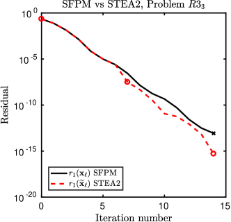
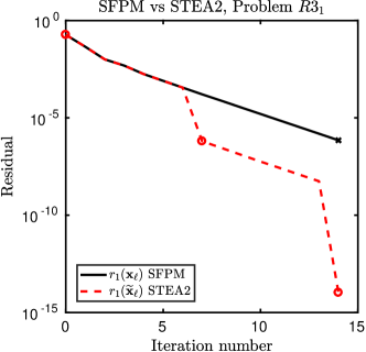
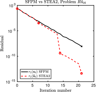
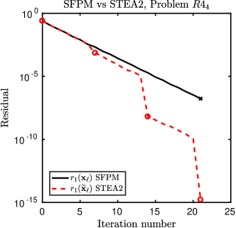
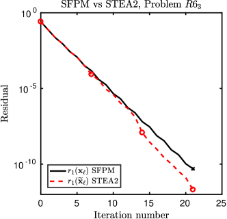
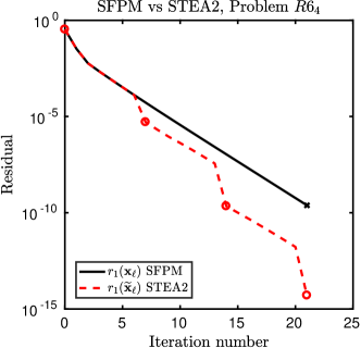
Figure 1: $\alpha=0.499\;\gamma=0$ Left column: worst acceleration performance, obtained on problems $R3_{3},\;R4_{16},\;R6_{3}$ (top-bottom). Right column: best acceleration performance, obtained on problems $R3_{1},\;R4_{4},\;R6_{4}$ (top-bottom).

4.1 Problem Set 1

In this section we use the benchmark set of 29 problems used in [32, 42] that consists of order-$3$ $n\times n\times n$ stochastic tensors where $n=3,4,6$.

   
   

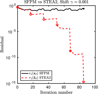
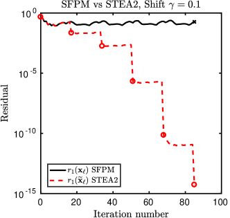
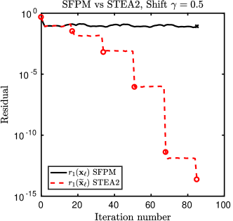
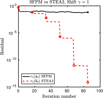
Figure 2: $\alpha=0.99$. Performance obtained on problem $R4_{19}$ for $\gamma\in\{0.001,0.1,0.5,1\}$.

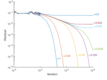
Figure 3: Results from [32] on the test problem $R4_{19}$ for different values of $\gamma$.

4.1.1 Extrapolated shifted power method

We tested Algorithm 1 on all the problems and, in Figure 1, we report for every $n=3,4,6$, the best and the worst speed-up performance (in terms of computed residuals) for the shifted power method coupled with the restarted extrapolation method when $\alpha=0.499$ and $\gamma=0$. The choices of the parameters $2k$ and $\mathsf{cycles}$ in Algorithm 1 are, respectively, $2k=6$ and $\mathsf{cycles}=2$ or $\mathsf{cycles}=3$.

As it is clear from these results, using extrapolation techniques considerably improves the performance of the shifted power method for the multilinear PageRank computation when $\alpha<1/2$. Observe, moreover, that the usage of extrapolation techniques is useful even when $\alpha$ is out of the range of convergence as Figure 2 shows ($2k=16$, $\mathsf{cycles}=5$). In that figure, we report detailed results for the test problem $R4_{19}$ from [32]. This problem is particularly challenging to solve when $\gamma\leq 0.5$ and, indeed, it is shown in [32] that for this range of the shifting parameter the power method fails to converge even after $10^{6}$ iterations. For completeness, we report in Figure 3 the corresponding results from the original paper. As shown by Figure 2, the relevance of the extrapolation framework introduced is particularly clear in this case as, on the other hand, the extrapolated iterations converge even for very small values of $\gamma$.

In order to have a more precise idea of the effectiveness of our approach, in Table 1 we report the number of “solved” problems when $\alpha=0.99$ and $\gamma=1$. We say that a problem is “solved” if we are able to obtain a residual (22) less than $10^{-8}$. Here the choices of $2k$ and $\mathsf{cycles}$ in Algorithm 1 range, respectively, between $6-20$ and $6-12$.

	Solved Problems
$n=3$	4/5
$n=4$	15/19
$n=6$	3/5
Total	22/29

Table 1: Performance for $\alpha=0.99$ and $\gamma=1$.

4.1.2 Extrapolated inner-outer

In the previous Section 4.1.1 we showed that the introduction of the simplified topological $\varepsilon$-algorithm in the shifted fixed-point method produces evident computational benefits for the solution of the multilinear PageRank problems in both the cases when $\alpha$ is inside or outside the range of convergence. The inner-outer method, at each iteration, solves a multilinear PageRank problem with $\alpha$ inside the convergence range (see (11)); for this reason we strongly recommend the employment of extrapolation techniques in each inner step of the inner-outer method when solved with the shifted fixed-point method. Nevertheless, one could wonder whether the extrapolation strategy can speed-up not only the computations for the solution of each inner step of the inner-outer iteration, but also the convergence of the outer sequence. The results presented in this section address this issue.

   
   
   

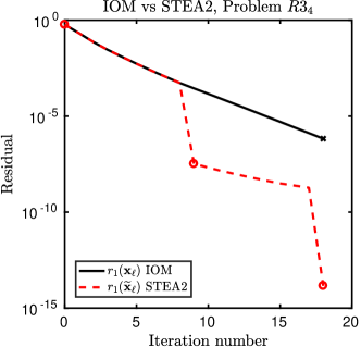
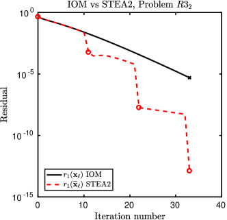
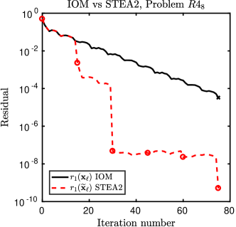
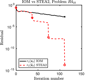
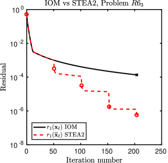
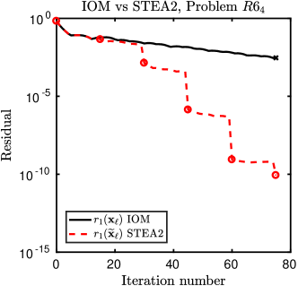
Figure 4: $\alpha=0.99.$ Left column: worst acceleration performance, obtained on problems $R3_{4},\;R4_{8},\;R6_{3}$ (top-bottom). Right column: best acceleration performance, obtained on problems $R3_{2},\;R4_{10},\;R6_{4}$ (top-bottom). $R6_{3}$ not solved.

In Figure 4, we report best and worst performance of the inner-outer iteration (11) with $\alpha=0.99$ when coupled with the restarted extrapolation method. We successfully solve all the problems in our set except for problem $R6_{3}$. The choices of the parameters $2k$ and $\mathsf{cycles}$ in Algorithm 1 range between $10-50$ and $3-9$, respectively.

4.2 Problem Set 2

In order to generate stochastic order-$m$ tensors of any desired dimension $n$ and produce statistics on a large number of datasets with different sizes, we consider the following procedure which uses the random graph generator CONTEST [52]:

Algorithm 2 Stochastic Tensor generator

$n$ (size of the tensor), $m$ (modes of the tensor),

${\bf g}=\{\mathtt{smallw}(n),\mathtt{gilbert}(n),\mathtt{erdrey}(n),\mathtt{pref}(n),\mathtt{geo}(n),\mathtt{lockandkey}(n),\mathtt{rank1}(n)\}$

for $i=1,\dots,n^{m-2}$ do

     Choose randomly an element ${\bf g}_{r}$ of ${\bf g}$

     Set ${P}_{:\,,\,n(i-1)+1:in}={\bf g}_{r}$

     Transform ${P}_{:\,,\,n(i-1)+1:in}$ into a stochastic matrix by rescaling the columns

end for

Output: $\mathcal{P}$ is the $m$-th order stochastic tensor whose stochastic unfolding is $P$.

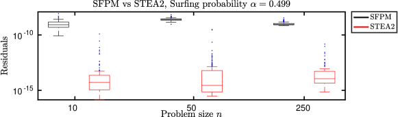
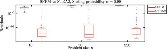
Figure 5: Median and quartiles of SFPM and STEA2 after $(2k+1)\times\mathsf{cycles}$ iterations on $100$ random tensors obtained by Algorithm 2, with $\alpha=0.499$, $\gamma=0$, $2k=10,\;\mathsf{cycles}=2$, $n=10,50,250$ and $m=2$.

Figure 6: Median and quartiles of SFPM and STEA2 after $(2k+1)\times\mathsf{cycles}$ iterations on $100$ random tensors obtained by Algorithm 2, with $\alpha=0.99$, $\gamma=1$, $2k=28,\;\mathsf{cycles}=4$, $n=10,50,250$ and $m=2$.

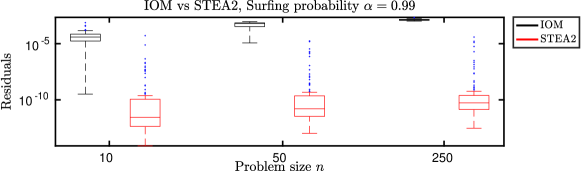
Figure 7: Median and quartiles of IOM and STEA2 after $(2k+1)\times\mathsf{cycles}$ iterations on $100$ random tensors obtained by Algorithm 2, with $\alpha=0.99$, $2k=32,\;\mathsf{cycles}=4$, $n=10,50,250$ and $m=2$.

In the above procedure, the symbols

$$\mathtt{smallw}(n),\,\mathtt{gilbert}(n),\,\mathtt{erdrey}(n),\,\mathtt{pref}(n),\,\mathtt{geo}(n),\,\mathtt{lockandkey}(n),$$

denote random adjacency matrices of dimension $n$ generated according to different random graph models described in the CONTEST package, whereas $\mathtt{rank1}(n)$ is the rank one matrix of all ones introduced in order to endow the tensor with a “strong directionality” feature which makes problems harder to be solved, as discussed in [32]. In this way it is possible to provide statistics about the acceleration performance of the proposed techniques and investigate the dependence on the parameter $2k$ in Algorithm 1 for increasing values of $n$ and $m$. As the obtained numerical results confirm, also in this case the use of extrapolation techniques significantly improves the performance of the shifted fixed-point method and of the inner-outer method. The analysis carried out here highlights a very weak dependence between the number of vectors used to perform the extrapolation, i.e., the choice of $2k$ in Algorithm 1, and the dimension of the problems. This feature demonstrates that the proposed technique is particularly effective for solving problems of large scale. This is further supported by the analysis on large scale real-world data carried out in the next Section 4.3.

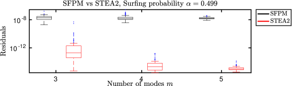
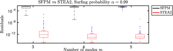
Figure 8: Median and quartiles of SFPM and STEA2 after $(2k+1)\times\mathsf{cycles}$ iteration on $100$ random tensors obtained by Algorithm 2, with $\alpha=0.499$, $\gamma=0$, $2k=8,\;\mathsf{cycles}=2$, $n=10$ and $m=3,4,5$.

Figure 9: Median and quartiles of SFPM and STEA2 after $(2k+1)\times\mathsf{cycles}$ iteration on $100$ random tensors obtained by Algorithm 2, with $\alpha=0.99$, $\gamma=1$, $2k=22,\;\mathsf{cycles}=4$, $n=10$ and $m=3,4,5$.

In Figure 6 we show results, via Matlab’s boxplots, on the acceleration performance of the shifted power method for the following choices of the parameters: $\alpha=0.499$, $\gamma=0$, $2k=10$ $\mathsf{cycles}=2$, $n=10,50,250$ and $m=2$. In particular, we show median and quartiles for the residual (22) after $(2k+1)\times\mathsf{cycles}$ iterations on 100 random example tests for both the shifted power method (in black) and the extrapolated sequence of Algorithm 1 (in red). In Figure 6, we show analogous results for the following choices of the parameters: $\alpha=0.99$, $\gamma=1$, $2k=28,\;\mathsf{cycles}=4$, $n=10,50,250$ and $m=2$. Whereas, in Figure 7, we report the results of the acceleration performance with respect to the inner-outer method for the following choices of the parameters: $\alpha=0.99$, $2k=32,\;\mathsf{cycles}=4$, $n=10,50,250$ and $m=2$.

Finally, Figures 9 and 9, show how the acceleration performance of the shifted fixed-point method varies when the number of modes of the tensor increases. The choices of the parameters are the following: $n=10$, $\alpha=0.499$, $\gamma=0$, $2k=8$, $\mathsf{cycles}=2$ or $\alpha=0.99$, $\gamma=1$, $2k=22$, $\mathsf{cycles}=4$ and $m=3,4,5$.

Figures 6-9 clearly show that the number of problems for which the proposed extrapolated algorithm provides major acceleration performance does not significantly change when $k$ and $\mathsf{cycles}$ in Algorithm 1 are fixed and either $n$ or $m$ increase. The independence of the parameter $k$ from the dimension $n$ and the number of modes $m$ is of utmost importance as this allows us to efficiently apply the proposed algorithm to large scale problems. This is also confirmed by real-world experiments of Section 4.3.

4.3 Real-world datasets

In this section we report experimental results of the extrapolated shifted fixed-point method when applied to a number of real world datasets borrowed from [22, 34]. Precisely, given an undirected graph $G$ with $n$ nodes, we generate the third-order symmetric tensor $\mathcal{C}$ defined as follows

$$\mathcal{C}_{i,j,k}=\begin{cases}1,\hbox{ if there is a three-cycle between nodes }i,j,k\\ 0,\hbox{ otherwise.}\end{cases}\,$$

Problem name	Source	Size	nnz(A)	nnz($\mathcal{C}$)		Problem name	Source	Size	nnz(A)	nnz($\mathcal{C}$)
Bristol∗	[34]	2892	9076	7722		minnesota	[22]	2642	6606	318
Cardiff∗	[34]	2685	8888	15186		NotreDame_yeast	[22]	2114	4480	2075
Edinburgh∗	[34]	1645	4292	1404		p2p-Gnutella04∗	[22]	10879	79988	5604
Glasgow∗	[34]	1802	4568	1458		USpwerGrid	[22]	4941	13188	3906
Nottingham∗	[34]	2066	6310	6162		wiki-Vote∗	[22]	8297	201524	3650334
Erdos02	[22]	6927	16944	14430		wing_nodal	[22]	10937	150976	803082
EX6	[22]	6545	295680	1774080		yeast	[22]	2361	13828	35965

Table 2: Datasets’ information

		STEA2			SFPM
	$\beta$	Time(s)	Iter	Res	Time(s)	Iter	Res
Bristol	0.1	4.28	93	8.64e-10	8.13	199	9.42e-09
	0.3	1.70	38	2.80e-09	3.27	79	9.07e-09
	0.6	1.21	27	1.09e-09	1.80	41	9.65e-09
Cardiff	0.1	3.91	93	6.35e-09	7.47	206	9.91e-09
	0.3	1.48	38	5.83e-09	2.96	81	8.89e-09
	0.6	1.06	27	3.45e-10	1.54	42	7.51e-09
Edinburgh	0.1	1.67	93	2.84e-09	2.75	205	9.62e-09
	0.3	0.40	38	2.48e-09	0.61	81	8.75e-09
	0.6	0.42	27	1.56e-09	0.56	42	8.27e-09
Glasgow	0.1	3.23	155	6.64e-09	3.31	206	9.46e-09
	0.3	0.72	57	5.45e-10	0.78	81	9.08e-09
	0.6	0.46	27	7.58e-10	0.71	42	8.82e-09
Nottingham	0.1	4.11	155	3.86e-09	4.34	206	9.42e-09
	0.3	0.98	38	1.93e-09	1.85	81	8.43e-09
	0.6	0.69	27	1.17e-10	0.90	42	7.53e-09
Erdos02	0.1	29.61	124	8.02e-10	37.64	165	9.82e-09
	0.3	13.82	57	1.31e-09	17.12	73	8.70e-09
	0.6	6.54	27	4.50e-09	9.00	39	9.16e-09
EX6	0.1	6.95	31	2.40e-09	13.73	63	8.84e-09
	0.3	10.31	38	2.90e-11	11.40	46	9.11e-09
	0.6	6.28	27	1.21e-10	7.93	32	9.38e-09
minnesota	0.1	4.91	124	1.71e-09	7.56	221	9.47e-09
	0.3	1.41	38	8.43e-09	2.87	84	8.51e-09
	0.6	0.96	27	3.73e-10	1.48	43	7.37e-09
ND_yeast	0.1	2.70	155	5.56e-09	2.95	229	9.52e-09
	0.3	1.47	57	2.52e-11	1.82	85	9.71e-09
	0.6	0.45	27	4.21e-09	0.55	43	8.51e-09
p2p-Gnutella04	0.1	35.91	62	5.18e-09	71.63	127	9.96e-09
	0.3	22.44	38	2.32e-09	31.28	55	9.05e-09
	0.6	15.82	27	7.84e-10	20.02	35	7.75e-09
USpowerGrid	0.1	19.36	155	3.20e-09	25.94	210	9.65e-09
	0.3	4.78	38	1.96e-09	9.73	82	8.67e-09
	0.6	3.34	27	5.58e-10	5.01	42	9.11e-09
wiki-Vote	0.1	32.32	93	1.39e-10	57.22	170	9.72e-09
	0.3	13.10	38	1.37e-09	23.41	65	8.61e-09
	0.6	9.22	27	9.83e-10	11.95	36	8.85e-09
wing_nodal	0.1	54.76	93	6.15e-10	106.82	187	9.43e-09
	0.3	22.38	38	7.94e-09	42.43	74	9.23e-09
	0.6	12.09	18	3.22e-09	22.09	39	8.06e-09
yeast	0.1	3.06	93	1.20e-09	5.81	212	9.97e-09
	0.3	0.69	38	1.59e-09	1.31	79	9.22e-09
	0.6	0.80	27	4.53e-09	1.14	41	7.24e-09

Table 3: Performance on the real-world datasets of Table 2

Following the construction proposed in [2, 32], we transform $\mathcal{C}$ into a new stochastic tensor $\mathcal{R}$ as follows. Let $S$ be the mode-one unfolding of $\mathcal{C}$ that has been normalized to be a sub-stochastic matrix by scaling its columns, let $A$ be the adjacency matrix of $G$ and let $D$ be the diagonal matrix of the degrees of $G$, $D_{ii}=\sum_{j}A_{ij}$. Finally, let $M=A^{T}D^{+}$, where $D^{+}$ is the Moore-Penrose pseudoinverse of $D$. We define $\mathcal{R}$ as the order-3 tensor whose mode-1 unfolding is

$$R=\beta[S+\mathbf{v}\,\mathrm{dangling}(S)]+(1-\beta)[M+\mathbf{v}\,\mathrm{dangling}(M)]\otimes\mathbf{e}\,,$$ (23)

where $0\leq\beta\leq 1$, $\mathbf{v}\in\Omega_{+}$ is a positive stochastic vector and where, for a matrix $B\in\mathbb{R}^{n\times n}$ and the all-ones vector $\mathbf{e}$, we let $\mathrm{dangling}(B):=\mathbf{e}^{T}-\mathbf{e}^{T}B$.

We report in Table 2 the details of the graphs we took into account; when the graph $G$ is directed – marked with an asterisk – we considered its undirected version: if $A$ is the adjacency matrix of $G$, we consider the graph $G^{\prime}$ corresponding to the adjacency matrix $A^{\prime}=\mathrm{sign}(A+A^{T})$, whose entries are $(A^{\prime})_{ij}=\mathrm{sign}(a_{ij}+a_{ji})$. In Table 3 we report the obtained numerical results when $\alpha=0.99$, $\gamma=1$, $2k=8$ if $\beta=0.6$, $2k=18$ if $\beta=0.3$ and $2k=30$ if $\beta=0.1$.

Let us stress that the execution times we report here include the running time of the extrapolation routines. It is possible to clearly appreciate the computational benefits resulting from the introduction of the extrapolation techniques: the computational times and the number of iterations needed to produce a residual not larger than $10^{-8}$ are always reduced; for some problems, for which the shifted fixed-point method is particularly slow ($\beta=0.1$), the iterations and the execution times reduce dramatically, up to the 230%, obtained for the dataset “yeast”. We highlighted in bold the most relevant speed-up performance in Table 3.

5 Conclusions

We showed that the use of extrapolation techniques for the computation of the multilinear PageRank using fixed-point iterations improves substantially the efficiency and effectiveness on the test problems we considered at a limited additional cost. In particular, we have shown that extrapolated versions of the shifted power and inner-outer methods are able to solve certain pathological test problems where the original methods consistently fail. Moreover, the performance of the methods (in terms of execution time) remarkably improves, allowing to address very large problems. Finally, let us point out that, as it is formulated, the multilinear PageRank problem is equivalent to the computation of a $Z$-eigenvector of a stochastic tensor for which the shifted power method introduced in [38] can be used. In that work the authors observed that the shifted power method could suffer of an extremely low rate of convergence affecting its employment in large scale applications. For this reason, they have raised the issue regarding the possibility of suitably speeding-up the shifted power method. The numerical results obtained and presented in this work allow us to answer positively to their question when the shifted power method is used for the computation of the multilinear PageRank solution and is coupled with the Simplified Topological $\varepsilon$-algorithm, encouraging the numerical community to use the proposed techniques when dealing with problems similar to those presented here. We intend to come back to the theoretical analysis concerning the justification of the remarkable acceleration performance obtained here in a forthcoming work.

References

- [1] F. Arrigo and F. Tudisco. Multi-dimensional, multilayer, nonlinear and dynamic hits. In Proceedings of the SIAM International Conference on Data Mining. SIAM, in press.
- [2] A. R. Benson, D. F. Gleich, and J. Leskovec. Tensor spectral clustering for partitioning higher-order network structures. In Proceedings of the 2015 SIAM International Conference on Data Mining, pages 118–126. SIAM, 2015.
- [3] A. R. Benson, D. F. Gleich, and L. Lim. The Spacey Random Walk: a stochastic process for higher-order data. SIAM Rev., 59(2):321–345, 2017.
- [4] P. Berkhin. A survey on PageRank computing. Internet Math., 2(1):73–120, 2005.
- [5] A. Bouhamidi, K. Jbilou, L. Reichel, and H. Sadok. An extrapolated TSVD method for linear discrete ill-posed problems with Kronecker structure. Linear Algebra Appl., 434(7):1677–1688, 2011.
- [6] H. Bozorgmanesh and M. Hajarian. Convergence of a transition probability tensor of a higher-order markov chain to the stationary probability vector. Numerical Linear Algebra with Applications, 23(6):972–988, 2016.
- [7] C. Brezinski. Généralisations de la transformation de Shanks, de la table de Padé et de l’-algorithme. Calcolo, 12(4):317–360, 1975.
- [8] C. Brezinski and M. Redivo-Zaglia. Extrapolation methods. Theory and Practice. North-Holland, Amsterdam, 1991.
- [9] C. Brezinski and M. Redivo-Zaglia. The PageRank vector: properties, computation, approximation, and acceleration. SIAM J. Matrix Anal. Appl., 28(2):551–575, 2006.
- [10] C. Brezinski and M. Redivo-Zaglia. Rational extrapolation for the PageRank vector. Math. Comp., 77(263):1585–1598, 2008.
- [11] C. Brezinski and M. Redivo-Zaglia. The simplified topological -algorithms for accelerating sequences in a vector space. SIAM J. Sci. Comput., 36(5):A2227–A2247, 2014.
- [12] C. Brezinski and M. Redivo-Zaglia. EPSfun: a Matlab toolbox for the simplified topological -algorithm. Netlib (http://wwww.netlib.org/numeralgo/), na44 package, 2017.
- [13] C. Brezinski and M. Redivo-Zaglia. The simplified topological -algorithms: software and applications. Numer. Algorithms, 74(4):1237–1260, 2017.
- [14] C. Brezinski, M. Redivo-Zaglia, G. Rodriguez, and S. Seatzu. Extrapolation techniques for ill-conditioned linear systems. Numer. Math., 81(1):1–29, 1998.
- [15] C. Brezinski, M. Redivo-Zaglia, and Y. Saad. Shanks sequence transformations and Anderson Acceleration. SIAM Rev., 60(3):626–645, 2018.
- [16] C. Brezinski, M. Redivo-Zaglia, and S. Serra-Capizzano. Extrapolation methods for PageRank computations. C. R. Math., 340(5):393–397, 2005.
- [17] K. Chang and T. Zhang. On the uniqueness and non-uniqueness of the positive z-eigenvector for transition probability tensors. Journal of Mathematical Analysis and Applications, 408(2):525–540, 2013.
- [18] K.-C. Chang, K. Pearson, and T. Zhang. Perron-Frobenius theorem for nonnegative tensors. Comm. Mathematical Sci., 6(2):507–520, 2008.
- [19] M. Chertok and Y. Keller. Efficient high order matching. IEEE Trans. Pattern. Anal. Mach. Intell., 32(12):2205–2215, 2010.
- [20] P. G. Ciarlet. Linear and nonlinear functional analysis with applications, volume 130. Siam, 2013.
- [21] S. Cipolla, C. Di Fiore, and F. Tudisco. Euler-Richardson method preconditioned by weakly stochastic matrix algebras: a potential contribution to Pagerank computation. Electron. J. Linear Algebra, 32:254–272, 2017.
- [22] T. A. Davis and Y. Hu. The University of Florida sparse matrix collection. ACM Trans. Math. Software, 38(1):1, 2011.
- [23] G. M. Del Corso, A. Gulli, and F. Romani. Fast PageRank computation via a sparse linear system. Internet Math., 2(3):251–273, 2005.
- [24] R. Durrett. Essentials of stochastic processes (2nd edn.), volume 1 of Springer Texts in Statistics. Springer, 2012.
- [25] D. Fasino and F. Tudisco. Higher-order ergodicity coefficients for stochastic tensors. Submitted, 2019.
- [26] S. Friedland, S. Gaubert, and L. Han. Perron–Frobenius theorem for nonnegative multilinear forms and extensions. Linear Algebra App., 438(2):738–749, 2013.
- [27] A. Gautier and F. Tudisco. The contractivity of cone–preserving multilinear mappings. IOP-LMS Nonlinearity, In press.
- [28] A. Gautier, F. Tudisco, and M. Hein. The Perron-Frobenius theorem for multi-homogeneous mappings. SIAM J. Matrix Anal Appl, In press.
- [29] A. Gautier, F. Tudisco, and M. Hein. A unifying Perron-Frobenius theorem for nonnegative tensors via multi-homogeneous maps. SIAM J. Matrix Anal Appl, In press.
- [30] D. F. Gleich. Pagerank beyond the web. SIAM Review, 57:321–363.
- [31] D. F. Gleich, A. P. Gray, C. Greif, and T. Lau. An inner-outer iteration for computing PageRank. SIAM J. Sci. Comput., 32(1):349–371, 2010.
- [32] D. F. Gleich, L.-H. Lim, and Y. Yu. Multilinear PageRank. SIAM J. Matrix Anal. Appl., 36(4):1507–1541, 2015.
- [33] G. H. Golub and C. Greif. An Arnoldi-type algorithm for computing pagerank. BIT, 46(4):759–771, 2006.
- [34] P. Grindrod and T. Lee. Comparison of social structures within cities of very different sizes. Roy. Soc. Open Sci., 3(2):150526, 2016.
- [35] S. Kamvar, T. Haveliwala, and G. Golub. Adaptive methods for the computation of pagerank. Linear Algebra Appl., 386:51–65, 2004.
- [36] S. D. Kamvar, T. H. Haveliwala, C. D. Manning, and G. H. Golub. Extrapolation methods for accelerating PageRank computations. In Proceedings of the 12th international conference on World Wide Web, pages 261–270. ACM, 2003.
- [37] E. Kofidis and P. A. Regalia. On the best rank-1 approximation of higher-order supersymmetric tensors. SIAM J. Matrix Anal. Appl., 23(3):863–884, 2002.
- [38] T. G. Kolda and J. R. Mayo. Shifted power method for computing tensor eigenpairs. SIAM J. Matrix Anal. Appl., 32(4):1095–1124, 2011.
- [39] H. Le Ferrand. The quadratic convergence of the topological epsilon algorithm for systems of nonlinear equations. Numer. Algorithms, 3(1):273–283, 1992.
- [40] W. Li, D. Liu, M. K. Ng, and S.-W. Vong. The uniqueness of multilinear PageRank vectors. Numer. Linear Algebra App., 24(6), 2017.
- [41] W. Li and M. K. Ng. On the limiting probability distribution of a transition probability tensor. Linear Multilinear Algebra, 62(3):362–385, 2014.
- [42] B. Meini and F. Poloni. Perron-based algorithms for the multilinear PageRank. Numer. Linear Algebra Appl., 0(0):2177.
- [43] M. Ng, X. Li, and Y. Ye. Multirank: co-ranking for objects and relations in multi-relational data. In Proceedings of the 17th ACM SIGKDD International conference on Knowledge Discovery and Data Mining, pages 1217–1225, 2011.
- [44] M. Ng, L. Qi, and G. Zhou. Finding the largest eigenvalue of a nonnegative tensor. SIAM J. Matrix Anal. Appl., 31(3):1090–1099, 2009.
- [45] Q. Nguyen, F. Tudisco, A. Gautier, and M. Hein. An efficient multilinear optimization framework for hypergraph matching. IEEE Trans. Pattern. Anal. Mach. Intell., 39(6):1054–1075, 2017.
- [46] L. Page, S. Brin, R. Motwani, and T. Winograd. The PageRank citation ranking: Bringing order to the web. Technical report, Stanford InfoLab, 1999.
- [47] M. Saburov. Ergodicity of -majorizing nonlinear Markov operators on the finite dimensional space. Linear Algebra Appl., 578:53–74, 2019.
- [48] S. Serra-Capizzano. Jordan canonical form of the Google matrix: a potential contribution to the PageRank computation. SIAM J. Matrix Anal. Appl., 27(2):305–312, 2005.
- [49] D. Shanks. Non-linear transformations of divergent and slowly convergent sequences. J. Math. Phys., 34(1-4):1–42, 1955.
- [50] A. Shashua and T. Hazan. Non-negative tensor factorization with applications to statistics and computer vision. In Proceedings of the 22nd International Conference on Machine learning, pages 792–799. ACM, 2005.
- [51] S. Soltani, M. E. Kilmer, and P. C. Hansen. A tensor-based dictionary learning approach to tomographic image reconstruction. BIT, 56(4):1425–1454, 2016.
- [52] A. Taylor and D. J. Higham. Contest: A controllable test matrix toolbox for Matlab. ACM Trans. Math. Software, 35(4):26, 2009.
- [53] F. Tudisco, F. Arrigo, and A. Gautier. Node and layer eigenvector centralities for multiplex networks. SIAM J. Appl. Math., 78(2):853–876, 2018.
- [54] F. Tudisco, V. Cardinali, and C. Di Fiore. On complex power nonnegative matrices. Linear Algebra App., 471:449–468, 2015.
- [55] F. Tudisco and C. Di Fiore. A preconditioning approach to the pagerank computation problem. Linear Algebra and its Applications, 435(9):2222–2246, 2011.
- [56] R. S. Varga. Matrix iterative analysis, volume 27. Springer Science & Business Media, 2009.
- [57] S. Wu and M. T. Chu. Markov chains with memory, tensor formulation, and the dynamics of power iteration. App. Math. Comput., 303:226–239, 2017.
- [58] P. Wynn. On a device for computing the transformation. MTAC, pages 91–96, 1956.