The $\Lambda$-invariant and topological pathways to influence sub-micron strength and crystal plasticity

Abstract

In small volumes, sample dimensions are known to strongly influence mechanical behavior, especially strength and crystal plasticity. This correlation fades away at the so-called mesoscale, loosely defined at several micrometers in both experiments and simulations. However, this picture depends on the entanglement of the initial defect configuration. In this paper, we study the effect of sample dimensions with a full control on dislocation topology, through the use of a novel observable for dislocation ensembles, the $\Lambda$-invariant, that depends only on mutual dislocation linking: It is built on the natural vortex character of dislocations and it has a continuum/discrete correspondence that may assist multiscale modeling descriptions. We investigate arbitrarily complex initial dislocation microstructures in sub-micron-sized pillars, using three-dimensional discrete dislocation dynamics simulations for finite volumes. We demonstrate how to engineer nanoscale dislocation ensembles that appear virtually independent from sample dimensions, either by biased-random dislocation loop deposition or by sequential mechanical loads of compression and torsion.

Among the most remarkable aspects of forming processes in metals is the ability to manipulate material strength by “cold working” Asaro and Lubarda (2006). At the heart of this versatile feature lies the ability of crystal defects, especially dislocations Anderson et al. (2017); Kubin (2013), to interact collectively, develop entangled microstructures and multiply. Dislocation entanglement has been notoriously believed to control a plethora of phenomena in metallurgy, including work and kinematic hardening, as well as fatigue Nabarro et al. (1964). However, the paramount importance of dislocation entanglement only became clear in the study of small finite volumes, by noticing the dramatic effects of its absence El-Awady et al. (2009); Lee et al. (2013); Ryu et al. (2015); Papanikolaou et al. (2017a, b, 2012): Crystalline strength drastically increases when at least one dimension decreases below the so-called mesoscale, which loosely refers to a few micrometers Croes (2011); Devincre et al. (2008); Bulatov et al. (2006); Kocks and Mecking (2003); Mecking and Kocks (1981) where dislocations, conceived as point particles, define their “mean-free path” Devincre et al. (2008). Nevertheless, crystal dislocations are more often than not, loops that may easily extend to the volume boundaries, and thus mutual dislocation topologies may be critical. In addition, far-from-equilibrium basics suggest that mechanical yielding is a transient behavior that ought to strongly depend on initial conditions, especially in small volumes Goldenfeld (1992). In this work, we show that dislocation entanglement primarily depends on the dislocation ensemble topology and not a particular lengthscale. We investigate the possible effects of initial conditions by constructing a topological observable of dislocation networks, the $\Lambda$-invariant, that is only dependent on mutual loop entanglement. We show that the $\Lambda$-invariant can be used to generate arbitrarily complex microstructures, either by deposition or cold-working, rendering a sub-micron volume capable of yielding like a bulk sample. In this way, we may identify topological pathways to manage strength and crystal plasticity and unify critical aspects of multiscale materials modeling.

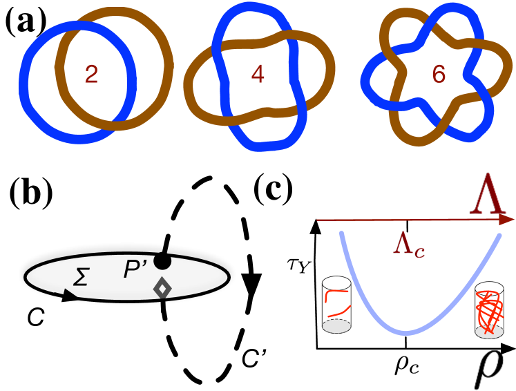
Figure 1: Dislocation Loops and Topology. (a) Two dislocation loops on different slip systems can form a topological link with linking number 2, 4 or 6 depending on the activation of additional latent hardening mechanisms such as double cross-slip. (b) The linking number can be directly calculated through a dislocation line double integral, the Gauss integral. (c) The calculation of a dislocation ensemble linking number (assuming closed dislocation loops) can be performed either in simulations or experiments (Figure).

While interactions and mechanisms of individual dislocations are fairly understood, crystal plasticity modeling still remains an enormous challenge. For example, the necessary “back-stress” for theories of kinematic and work hardening Asaro and Lubarda (2006), does not yet have a precise microscopic definition El-Azab (2000); Chen et al. (2010). In fact, the great complexity of crystal plasticity theories originates in that dislocation ensembles are more akin to a “bird’s nest”, rather than a set of separate small and simpler elementary bodies Cottrell et al. (2002). In sub-micron-sized volumes, where it becomes tough to fit such a nest, common plasticity practically disappears, giving its place to uncommon size effects and stochasticity in the mechanical response Dimiduk et al. (2006); Uchic et al. (2009a); Papanikolaou et al. (2017b). In association, cold-working a micropillar before testing El-Awady et al. (2011) may turn size effects into Taylor hardening (cf. Fig. 1(c)), as dislocation density increases El-Awady (2015). However, another plausible interpretation is that dislocation complexity is the key, in a small finite volume, that may unlock common plasticity. In such a scenario, the inflection point $\Lambda_{c}$ has a fundamental importance in terms of topological complexity, possibly revealing how many dislocation “twigs” need to intertwine to start behaving as a bird’s nest.

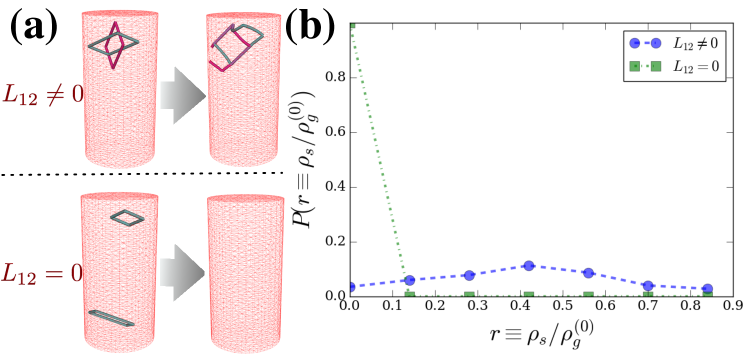
Figure 2: Energetics & Statistics: (a) Initial conditions of i) two prismatic dislocation loops 1 and 2, with randomly selected Burgers vectors but finite $L_{12}$, ii) two prismatic dislocation loops 1 and 2, with randomly selected Burgers vectors but zero $L_{12}$. (b) Probability of forming sessile dislocation junctions through 2 randomly placed prismatic loops with or without linking.

We present a novel approach to characterize and engineer dislocation entanglement that naturally translates into continuum and large-deformation descriptions of dislocation ensembles. Our basis is the construction of a scalar volume observable, dubbed $\Lambda$-invariant, which may be shown to have special topological properties, thus leaping beyond the distortion (elastic/plastic) or dislocation density tensors Hirth and Lothe (1982). The purpose of $\Lambda$ is to count and sum the linking number of each pair of dislocation loops across the ensemble.

The Linking Number for two dislocation loops $i$ and $j$ is defined as $L_{ij}=\frac{1}{4\pi}\int_{C_{1}}\int_{C_{2}}d\Omega({\bf r}_{1},{\bf r}_{2})\equiv\frac{1}{4\pi}\int_{C_{1}}\int_{C_{2}}\frac{(d{\bf r}_{2}\times{\bf r}_{1}){\bf r}_{12}}{r_{12}^{3}}$ Murasugi (2007); Kauffman (1991) and it is a plausible way to define the mutual entanglement of a pair of dislocation loops (cf. Fig. 1(b)). A linking number of 2 is typical for crossing dislocations in different slip systems, while higher linking numbers require additional consecutive mechanisms such as consercutive double cross-slip events (cf. Fig. 1(a)). The topological character of the linking number originates in that it does not depend on local line distortions, thus it does not explicitly relate to dislocation length density. In this way, it complements common dislocation network observables.

The $\Lambda$-invariant in a crystal of Burgers vector magnitude $b$ is defined as,

$$\Lambda=\frac{1}{b^{2}}\int d^{3}x\beta^{E}\cdot(\nabla\times\beta^{E})=\frac{1}{b^{2}}\int d^{3}x\beta^{E}_{ij}\alpha_{ij}$$ (1)

where $\alpha$ is the Nye dislocation density tensor and the elastic distortion $\beta^{E}$ combines with the plastic distortion $\beta^{P}$ to give $\beta^{P}+\beta^{E}=grad(u)$, where $u$ is the displacement field due to deformation Asaro and Lubarda (2006); Anderson et al. (2017), ultimately satisfying on a closed crystal boundary $\Gamma$

$$\alpha=\nabla\times\beta^{E}=-\nabla\times\beta^{P}=\delta_{\Gamma}\otimes\vec{b}$$ (2)

This defining vortex character of dislocations signifies that dislocations maintain a loop character that may not end within the crystal. By using this feature, one may show (see Appendix A) Moffatt et al. (2013); Moffatt (1969) that

$$\Lambda=-\frac{1}{b^{2}}\sum_{i,j}L_{ij}{\bf b}_{i}\cdot{\bf b}_{j}$$ (3)

where $L_{ij}$ is the linking number between loops $i$ and $j$, while ${\bf b}_{i}$ and ${\bf b}_{j}$ are their respective Burgers vectors.

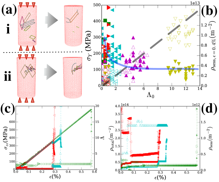
Figure 3: Depositing&Testing Entanglement – Uniaxial Compression in Designed Dislocation Configurations $\&$ Size In-dependence (a) Random deposition and uniaxial compression of prismatic dislocation loops in a finite mesh of $R=0.3\mu{\rm m}$ in (i) an unbiased or (ii) $\Lambda$-biased manner. (shown compression to $0.01\%$ strain for $\rho_{0}=2\times 10^{13}/{\rm m}^{2}$) (b) Nanopillar yield stress (solid symbols) and sessile dislocation density (open symbols) at $0.2\%$ strain as function of initial $\Lambda_{0}$. Every point corresponds to a uniaxial compression simulation: ($\rho_{0}:\{\blacksquare:10^{13}/{\rm m}^{2}\}$, $\{\blacktriangleright:2\times 10^{13}/{\rm m}^{2}\}$, $\{\blacktriangleleft:4\times 10^{13}/{\rm m}^{2}\}$, $\{\blacktriangle:8\times 10^{13}/{\rm m}^{2}\}$, $\{\blacktriangledown:10^{14}/{\rm m}^{2}\}$). Also, three sample cases are shown for (c) loading stress $\sigma_{\rm zz}$ and $\Lambda$ vs. $\epsilon$, and (d) total and sessile dislocation density vs. $\epsilon$. Sessile dislocation density increases roughly linearly with $\Lambda_{0}$ while yield stress quickly saturates. ($\{\blacktriangle:8\times 10^{12}/{\rm m}^{2}\}$, $\{\blacktriangleright:10^{13}/{\rm m}^{2}\}$, $\{\blacktriangleleft:2\times 10^{13}/{\rm m}^{2}\}$)

The primary usefulness of $\Lambda$ is its capacity of predicting the onset of dislocation multiplication through dislocation junction formation and associated mechanisms. The connection between finite $\Lambda$ and junction formation can be seen in two ways: First, the absence of linking ($L_{ij}=0$) leads to a negligible statistical probability for junction formation, especially in small finite volumes (cf. Fig. 2). Second, the dependence of $\Lambda$ on the linking loops’ Burgers vectors’ dot product point directly to a junction-formation energetic connection to the Frank rule. A way to realize different possibilities is to consider prismatic dislocation loops, which have been connected to hardening effects in various circumstances Püschl (2002); Saada and Washburn (1962). If one considers two prismatic dislocation loops randomly placed in a small finite volume, then the histogram of sessile dislocation junction formation displays significant junction length formation for both signs of $\Lambda$, with a wide probability distribution (see Fig. 2) that remarkably overwhelms the unlinking case. It is worth noting that it has been common to consider segment-based junction formation arguments Wickham et al. (1999); Madec et al. (2002a) (ie. nearby straight lines), but the scenario of two dislocation loops that intertwine is significantly different since all possible signs of dislocation interactions are present in such a linked dislocation pair. Thus, it is natural to expect a significantly larger statistical preference towards sessile junction formation for linked loops than two nearby straight lines Shenoy et al. (2000); Madec et al. (2002b)

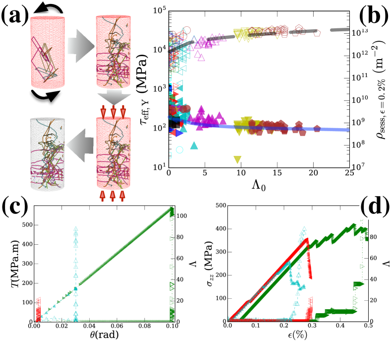
Figure 4: Engineering Entanglement by Cold Working: Pure Torsion Followed by Uniaxial Compression. (a) A protocol is followed where a dislocation loop configuration at density $\rho_{0}$ is prepared, torsion is applied on top/bottom pillar surfaces up to pre-chosen torsion angle $\theta_{0}$, and then uniaxial compression is applied towards yield. The configurations at each step of the process are shown for a particular configuration with $\rho_{0}=3\times 10^{13}/{\rm m}^{2}$. (b) Yield stress vs. $\Lambda_{0}$ for a variety of initial conditions and torsions $\rho_{0}\in(5\times 10^{12},2\times 10^{14})$ and $T\in\{10^{-5},0.1\}$. Three characteristic cases are shown for (c) Torsion $T$ (filled symbols) and $\Lambda$ (open symbols) vs. torsion angle $\theta$ and (d) subsequent loading stress $\sigma_{\rm zz}$ (filled symbols) and $\Lambda$ (open symbols) vs. axial strain $\epsilon$. $\{\rho_{0},\theta_{0}\}\rightarrow$($\blacktriangleright:[10^{13}/{\rm m}^{2},0.1]$, $\blacktriangleleft:[2\times 10^{13}/{\rm m}^{2},3\times 10^{-3}]$, $\blacktriangle:[2\times 10^{13}/{\rm m}^{2},3\times 10^{-2}]\Big{)}$.

The statistical finding for the fate of two linked loops has significant consequences for the behavior of collective dislocation networks. By using a numerical algorithm that explicitly tracks dislocation loops Po and Ghoniem (2015) and their mutual linking numbers throughout the dislocation dynamics simulation Ghoniem and Amodeo (1988); Arsenlis et al. (2007); Van der Giessen and Needleman (1995); Weygand et al. (2001); Po et al. (2014); Po and Ghoniem (2015), we are able to arbitrarily tune the complexity of the initially deposited dislocation configuration. We consider the geometry of a cylindrical nanopillar finite element mesh of diameter $D=2000b\sim 600$nm for single crystalline Cu FCC with ${\bf b}=0.185{\rm nm}$. We generate a wealth of prismatic loop initial conditions by depositing prismatic dislocation loops of randomly selected Burgers vectors in the nanopillar until a target dislocation density $\rho_{0}$ is reached (see e.g. Fig. 3(a) for $\rho_{0}=10^{13}/{\rm m}^{2}$). Furthermore, by biasing the deposition of prismatic loops towards collectively increasing $\Lambda$ magnitude, we acquire complete control on the investigation of dislocation topological effects.

The effect of topologically rich initial conditions is drastic in causing statistical size independence in material properties such as the compressive yield strength (cf. Fig. 3(b)). For large initial $\Lambda_{0}$ (in this work, we focus on $\Lambda$’s magnitude), in fact, the strength of the pillars is dominated by the microstructure entanglement as opposed to the sample size, leading to a linear increase of the sessile dislocation density at an arbitrarily chosen $0.4\%$ finite strain $(\rho_{sess}\sim\Lambda_{0})$. While this is only evidence of a scaling relation between $\Lambda_{0}$ and dislocation densities in small finite volumes, we expect that the scaling relationship $\rho_{sess}(\epsilon)\sim\Lambda_{0}^{\delta}$ for $\delta\geq 0$ generically holds for any dislocation ensemble. Plastic yielding in these systems is accompanied by large $\Lambda$-“avalanches” (cf. Fig. 3(c)), caused by large increase in the density of sessile (cf. Fig. 3(d)), and subsequent multiplication to increase the total dislocation density (cf. Fig. 3(d)). Overall, this behavior should be contrasted to the typically observed size-dependent one in analogously small finite volumes Uchic et al. (2009b), which in our simulations can be seen only for $\Lambda_{0}<1.8$.

Besides artificial deposition of initial dislocation configurations with dramatic effects on mechanical properties, the topological character of $\Lambda$ may guide us towards generating large-entanglement structures through particularly efficient mechanical loading paths. These loading paths can be also predicted through modeling of latent hardening for particular crystalline structure Lagneborg and Forsen (1973). The key towards identifying such loading paths is the calculation of the $\Lambda$-dynamics. For a large class of continuum dislocation theories that satisfy global Burgers vector conservation and Orowan’s law of collective dislocation motion, it may be shown that (Appendix B)

$$\frac{\partial\Lambda}{\partial t}=\frac{1}{b^{2}}\int_{\partial V}dS_{j}\epsilon_{jkm}\beta^{E}_{kl}J_{ml}$$ (4)

where the typical assumption of overdamped dynamics is considered and $J_{ij}=\epsilon_{ikm}F_{m}\alpha_{kj}$, where $F_{m}$ is the PK force on the dislocation density $\alpha_{kj}$. The tensorial character of the right-hand side of Eq. 4 implies that only particular loading directions can increase $\Lambda$, a fact well known from studies of latent hardening in crystal plasticity Devincre and Kubin (1994); Devincre et al. (2008); Kocks (1966); Takeuchi (1975). A physically intuitive example is the uniaxial compression of pre-torsioned specimens, where dislocation flow $J_{\rm ij}$ may be assumed in a pre-strained environment to a torsion angle $\theta_{0}$, with induced $\beta^{E}$ along the cylindrical $\theta$ direction (ie. $\partial_{x}u_{z}$ and $\partial_{y}u_{z}$ are non-zero) while ${\bf t}\times{\bf v}$ for an x-y gliding dislocation would be along ${\bf z}$ during compression. This combination of indices gives a concrete contribution to the right-hand-side integral of Eq. 4. Physically, in the idealized continuum cases, torsion induces geometrically imposed screw dislocations along the torsion axis. It is natural to expect that torsion-induced screw dislocations along the loading axis would tangle with horizontal-moving slip during subsequent compression, and this is precisely what Eq. 4 is predicting.

To confirm the approach towards the generation of $\Lambda$, we perform explicit 3D-DDD sequential-loading simulations of submicron-sized pillars with various initial dislocation densities $\rho_{0}$. We vary $\rho_{0}$ from $5\times 10^{12}$ to $3\times 10^{14}$. As shown in Fig. 4(a), the application of a finite amount of torsion (which may not be necessarily large enough to induce plasticity) on the top/bottom surfaces up to a target torsion angle $\theta_{0}$ ($\in(0,0.1)$rad), leads to a highly extended dislocation configuration that generates large entanglement when it is followed by uniaxial compression, as it is witnessed by the increase of $\Lambda$. Characteristically, if one calculates the combined-loading effective stress, then the yield stress is remarkably size-independent (cf. Fig. 4(b)) and the saturation level for the sessile dislocation density is easily at virtually any case, even with miniscule initial $\Lambda$ and initial dislocation density. As one may see in particular example cases (cf. Fig. 4(c),(d)), the application of torsion is followed with a dramatic increase of $\Lambda$, as suspected by our developed topological intuition.

The usefulness of $\Lambda$ is not limited to the characterization and prediction of discrete and entangled dislocation networks, but also it extends to represent a unique discrete-continuum link that can be directly calculated in both the discrete and the continuum worlds. In the continuum, it is just needed to properly estimate a $\beta^{E}$-dependent volume integral. Its topological origin also allows us to write the correspondent of $\Lambda$ for large deformations. Following Ref. Cermelli and Gurtin (2001) a large deformation generalization may be shown to be, (Appendix C)

$$\Lambda=\frac{1}{b^{2}}\int J^{e}{\bf F^{e-1}}\cdot(\nabla\times{\bf F^{e-1}})^{-\tau}\cdot{\bf F^{e-\tau}}d\tilde{V}$$ (5)

In this way, $\Lambda$’s information may be instrumental for extending dislocations’ role towards multiscale modeling of large scales and large deformations.

In conclusion, we presented a topological approach to investigate dislocation entanglement Devincre et al. (2006) and latent hardening in crystals. We find that the manipulation of initially prepared dislocation configurations’ topological complexity can generate size independent crystal plasticity even in nanoscale volumes, that are believed to be intrinsically size-dependent Voyiadjis and Yaghoobi (2017); Weinberger and Cai (2011). This leap of understanding on the manipulation and control of dislocation networks, may allow for optimization and design of multi-axial, sequential cold-working pathways in metallurgy.Hansen and Hughes (1995); Hong et al. (2013)

Appendix A $\Lambda$ and Linking Numbers

$$\oint_{\partial\mathcal{S}}\epsilon_{klm}TdL_{k}=\int_{\mathcal{S}}\left(T_{,m}dS_{l}-T_{,l}dS_{m}\right)$$ (6)

$$\oint_{\partial\mathcal{S}}TdL_{i}=\int_{\mathcal{S}}\epsilon_{ijk}T_{,k}dS_{j}$$ (7)

$$\frac{1}{4\pi}\oint\oint\frac{\bm{r}_{1}-\bm{r}_{2}}{\|\bm{r}_{1}-\bm{r}_{2}\|^{3}}\cdot(d\bm{r}_{1}\times d\bm{r}_{2})=$$

$$=\left(\frac{1}{R}\right)_{,j}\epsilon_{jkl}dx^{(A)}_{k}dx^{(B)}_{l}$$

$$=\frac{1}{2}R_{,ppj}\,\epsilon_{jkl}dx^{(A)}_{k}dx^{(B)}_{l}$$ (8)

$$b^{2}\Lambda = \int_{\mathbb{R}^{3}}\beta^{E}_{ij}\alpha_{ij}\,\text{d}V$$ (9)

$$= \int_{\mathbb{R}^{3}}\beta^{E}_{ij}\sum_{A}\oint_{\mathcal{L}^{A}}\delta(\bm{x}-\bm{x}^{\prime})b_{i}^{A}\,\text{d}\ell_{j}^{\prime}\,\text{d}V$$

$$= \sum_{A}b_{i}^{A}\oint_{\mathcal{L}^{A}}\beta^{E}_{ij}\,\text{d}\ell_{j}$$

$$= \sum_{A}b_{i}^{A}\oint_{\mathcal{L}^{A}}u_{i,j}\,\text{d}\ell_{j}\mp\sum_{A}b_{i}^{A}\oint_{\mathcal{L}^{A}}\beta^{P}_{ij}\,\text{d}\ell_{j}$$

$$= \sum_{A}b_{i}^{A}\oint_{\mathcal{L}^{A}}\sum_{B}\int_{\mathcal{S}^{B}}b^{B}_{i}\delta(\bm{x}-\bm{x}^{\prime})\,\text{d}S_{j}^{\prime}\,\text{d}\ell_{j}$$

$$= -\frac{1}{4\pi}\sum_{A}\sum_{B}b_{i}^{A}b^{B}_{i}\oint_{\mathcal{L}^{A}}\int_{\mathcal{S}^{B}}\left(\frac{1}{R}\right)_{,pp}\,\text{d}S_{j}^{\prime}\,\text{d}\ell_{j}$$

$$= -\frac{1}{4\pi}\sum_{A}\sum_{B}b_{i}^{A}b^{B}_{i}\oint_{\mathcal{L}^{A}}\int_{\mathcal{S}^{B}}\left(\frac{1}{R}\right)_{,pj}\,\text{d}S_{p}^{\prime}\,\text{d}\ell_{j}$$

$$-\frac{1}{4\pi}\sum_{A}\sum_{B}b_{i}^{A}b^{B}_{i}\oint_{\mathcal{L}^{A}}\oint_{\mathcal{L}^{B}}\epsilon_{kjp}\left(\frac{1}{R}\right)_{,p}\,\text{d}\ell_{k}^{\prime}\,\text{d}\ell_{j}$$

$$= -\frac{1}{4\pi}\sum_{A}\sum_{B}b_{i}^{A}b^{B}_{i}\oint_{\mathcal{L}^{A}}\oint_{\mathcal{L}^{B}}\epsilon_{kjp}\left(\frac{1}{R}\right)_{,p}\,\text{d}\ell_{k}^{\prime}\,\text{d}\ell_{j}^{\prime}$$

$$= -\sum_{A,B}L_{AB}{\bf b}_{A}\cdot{\bf b}_{B}$$

Appendix B The $\Lambda$ Dynamics

For x-y torsion $\beta_{E}\sim\hat{\theta}$ (primarily) in cylindrical coordinates, since most dislocations (screw) are lying along z-axis. Moreover, dynamics during compression in a torsioned specimen implies that $J\sim-\hat{r}$ in cylindrical coordinates. (to check it again)

In order to be careful, one needs to carefully perform these calculations using the proper tensorial indices. In this context, it is important to clarify that:

1. For $\alpha_{ij}$: $i$ indexes the dislocation line vector ${\bf t}$ that the dislocation is tangent to, while $j$ indexes the Burgers vector ${\bf b}$.

2. For $J_{ij}$ and a single dislocation line moving with velocity ${\bf v}$, $J_{ij}=\epsilon_{ikm}t_{k}b_{j}v_{m}\delta({\bf x})$ at some location ${\bf x}$. So, $i$ labels the cross product ${\bf t}\times{\bf v}$.

3. Also, for $J_{ij}$ (if overdamped dynamics is considered): it is written as $J_{ij}=\epsilon_{ikm}F_{m}\alpha_{kj}$, where $F_{m}$ is the PK force on the dislocation density $\alpha_{kj}$ ($F\times\alpha$ making sure that a dislocation density moves perpendicularly to the dislocation line vector).

4. For $\beta^{E}_{ij}$: $i$ labels the strain direction, while $j$ the component of the displacement vector.

5. We need to assume a particular dynamics law for the elastic and plastic distortion in order to proceed. Assuming the Nye dislocation tensor,

   $$\alpha_{ij}=-\epsilon_{ilm}\partial_{l}\beta^{P}_{mj}=\epsilon_{ilm}\partial_{l}\beta^{E}_{mj}$$ (10)

   we can assume a generic conservation law for the Burgers’ vector:

   $$\partial_{t}\alpha_{ij}=-\epsilon_{ilm}\partial_{l}J_{mj}$$ (11)

   which also implies,

   $$\partial_{t}\beta^{E}_{ij}=-J_{ij}$$ (12)

The ultimate target is to understand and predict which loading modes can lead to a large increase of the dislocation helicity, and consequently the elastic energy of the crystal. Assuming that the volume V is fixed, with $\partial V$ a boundary surface, then, if the helicity is defined as:

$$\Lambda=\frac{1}{b^{2}}\int_{V}dV\beta^{E}_{kl}\epsilon_{kmn}\partial_{m}\beta^{E}_{nl}$$ (13)

or

$$\Lambda=\frac{1}{b^{2}}\int_{V}dV\beta^{E}_{kl}\alpha_{kl}$$ (14)

then the temporal variation of dislocation helicity is derived by direct differentiation:

$$b^{2}\frac{\partial\Lambda}{\partial t}=\int_{V}dV\frac{\partial\beta^{E}_{kl}}{\partial t}\alpha_{kl}+\int_{V}dV\beta^{E}_{kl}\frac{\partial\alpha_{kl}}{\partial t}$$ (15)

Now we can use Eqs. 11 and 12, showing that

$$b^{2}\frac{\partial\Lambda}{\partial t}=-\int_{V}dVJ_{kl}\alpha_{kl}-\int_{V}dV\beta^{E}_{kl}\epsilon_{kjm}\partial_{j}J_{ml}$$ (16)

Now, we may use integration by parts in the second integral:

$$b^{2}\frac{\partial\Lambda}{\partial t}=-\int_{V}dVJ_{kl}\alpha_{kl}-\int_{\partial V}dS_{j}\beta^{E}_{kl}\epsilon_{kjm}J_{ml}+$$

$$\int_{V}dV\partial_{j}\beta^{E}_{kl}\epsilon_{kjm}J_{ml}$$ (17)

which is equal to:

$$b^{2}\frac{\partial\Lambda}{\partial t}=-\int_{V}dVJ_{kl}\alpha_{kl}-\int_{V}dV\alpha_{ml}J_{ml}-$$

$$\int_{\partial V}dS_{j}\beta^{E}_{kl}\epsilon_{kjm}J_{ml}$$ (18)

or

$$b^{2}\frac{\partial\Lambda}{\partial t}=-2\int_{V}dVJ_{kl}\alpha_{kl}+\int_{\partial V}dS_{j}\epsilon_{jkm}\beta^{E}_{kl}J_{ml}$$ (19)

The first integral (volume) is identically zero for the conservative dynamics, since $J_{kl}\alpha_{kl}=\epsilon_{kij}\alpha_{il}F_{j}\alpha_{kl}\equiv\epsilon_{kij}\alpha_{il}\alpha_{kl}F_{j}$ (zero by reversing k, i). Thus, it is proven that dislocation helicity is conserved by volume dynamics.

The second integral is equivalent to:

$$\int_{\partial V}d{\bf S}\cdot(\beta^{E}\times J)$$ (20)

Appendix C $\Lambda$ at large deformations

In the deformed configuration ${\bf x}$ (also labeled by above symbols), one can still define simply the burgers vector as a smooth loop/surface integral:

$${\bf b}=\int_{\partial S}{\bf F^{e-1}}d{\bf x}=\int_{S}(\nabla\times{\bf F^{e-1}})^{\tau}{\bf\tilde{n}}d\tilde{A}$$ (21)

with ${\bf F^{e-1}}=({\bf F^{e}})^{-1}$ and where ${\bf n}$ is the vector normal to the area S. Also, it is important to remember that,

$$(\nabla\times{\bf T})_{ij}=\epsilon_{irs}\frac{\partial T_{js}}{\partial x_{r}}$$ (22)

with respect to the orthonormal basis vectors.

At large deformations, it is important to remember that the deformed coordinates are connected to the reference configuration through the relation:

$$\tilde{\bf n}d\tilde{A}=J^{e}{\bf F^{e-\tau}}{\bf n}dA$$ (23)

Regarding the $\Lambda-$invariant, it is transparent how to extend our definitions in the large deformation regime, in the deformed coordinates. Namely, one can define,

$$\Lambda=\frac{1}{b^{2}}\int{\bf F^{e-1}}\cdot(\nabla\times{\bf F^{e-1}})^{-\tau}d\tilde{V}$$ (24)

and in the reference frame:

$$\Lambda=\frac{1}{b^{2}}\int J^{e}{\bf F^{e-1}}\cdot(\nabla\times{\bf F^{e-1}})^{-\tau}\cdot{\bf F^{e-\tau}}d\tilde{V}$$ (25)

Eq. 25 represents the large deformation definition of the $\Lambda-$invariant.