Construction of high precision numerical single and binary black hole initial data

Abstract

We present a novel implicit numerical implementation of the parabolic-hyperbolic formulation of the constraints of general relativity. The proposed method is unconditionally stable, has the advantage of not requiring the imposition of any boundary conditions in the strong field regime, and offers a holistic (all inclusive) approach to the construction of single and binary black hole initial data. The new implicit solver is extensively tested against known exact black hole solutions and is used to construct initial data for several single and binary black hole configurations.

I Introduction

With the observation of the signal GW151226 Collaboration and Collaboration (2016), general relativity officially entered the long-awaited era of observation of gravitational waves. This signal together with several others that have been observed to date Collaboration and Collaboration (2018) constitute the cornerstone of the emerging field of gravitational wave astronomy. The observed signals contain invaluable information about the physical properties of the merging binaries and the process of merging itself. The extraction of this information calls for the development of analytical and/or numerical methods that can reproduce the observed waveforms to the highest degree of accuracy. Due to the highly non-linear nature of the inspiral and merger of the binary systems that emitted the observed signals, the use of numerical methods is indispensable. During the last decade, following the seminal work of Pretorius Pretorius (2005), more and more sophisticated numerical models have been developed to simulate the dynamics of binary systems of massive compact objects. The accuracy of all these simulations crucially depends on their initialisation. It is expected that any failures or errors involved in the construction of the initial data sets will not only affect their subsequent temporal development but also the conclusions we can draw from it. Therefore, the construction of initial data for binary systems of massive astrophysical objects that are free from all sorts of defects—of analytical or numerical nature—is of paramount importance for numerical relativity. Especially today due to the key role of numerical relativity in simulating the gravitational waveforms emitted from binary systems of black holes or neutron stars.

In their entirety, the binary black hole initial data that have been constructed to date with any of the existing numerical methods contain some amount of “junk radiation”, i.e. pre-existing high frequency gravitational radiation that is not produced by the investigated binaries. Unfortunately, all the efforts that have been made to resolve this issue by modifying and/or refining the existing elliptic methods have not been successful. The presence of “junk radiation” in the initial data contaminates more or less, through their numerical evolution, the produced gravitational waveforms. Although the presence of “junk radiation” does not seem to affect the stability and convergence of the numerical codes, it affects to some extent the accuracy with which the parameters characterising the binary systems are estimated. (Recall that the parameters of a binary system—e.g. the mass, spin, etc.—are chosen in such a way that the numerically computed waveforms agree to a given precision with the observed gravitational wave signals.)

The origin of the “junk radiation” has been attributed to specific assumptions—i.e. maximal slicing condition, conformal flatness—made during the construction of the initial data with any of the available methods, see e.g. Alcubierre (2008). Moreover, recent work Chu (2014), relates also its presence to the use of excision. According to Chu (2014), the use of excision to place the inner boundary of the computational domain inside the event horizon distorts the tidal interactions between the black holes and leads to the creation of “junk radiation”. The results in Chu (2014) not only show a clear correlation between the use of excision and the presence of “junk radiation”, but also indicate that any approach that avoids the imposition of boundary conditions in the strong field regime could very well lead to a significant reduction of the ‘junk radiation” in the initial data. The above observations demonstrate the necessity of developing alternative methods of constructing initial data that are not bounded to the use of the above assumptions and techniques.

Recently, a completely novel formulation of Einstein’s constraint equations that fulfils all the aforementioned requirements was put forward by Rácz Rácz (2015). In the context of this formulation, a $2+1$ decomposition of the constraints is performed in a way that they can be viewed as an evolutionary system: parabolic-hyperbolic or algebraic-hyperbolic. Accordingly, one of the spatial coordinates, let’s say $z$, plays the role of the temporal coordinate along which the initial data, prescribed on the 2-dimensional surface composed by the remaining two spatial coordinates, are evolved. Exactly this feature is that disengages us from the “junk radiation”-generating assumptions used in the various variations of the elliptic York-Lichnerowicz method. Moreover, in this setting the use of excision is not required even in the case we are slicing through the event horizon of a black hole, see Fig. 1 for more details. These extremely appealing features of the $2+1$ formulation of the constraints make the construction of initial data with significantly reduced or entirely suppressed “junk radiation” highly doable.

The use of the assumptions of maximal slicing, conformal flatness, and purely longitudinal Bowen-York extrinsic curvature in the construction of the initial data is not only responsible for the generation of “junk radiation” in these data, but also restricts considerably the spectrum of the possible black hole initial data that can be constructed. For example the condition of conformal flatness excludes immediately the possibility of constructing any stationary Kerr type black hole initial data. Rácz’s method, on the other hand, is not bounded to the above assumptions and for this it can be used to generate any physically admissible single and binary black hole initial data.

In addition to the above extremely pleasant features, the parabolic-hyperbolic formulation offers a holistic (all inclusive) approach to the construction of both single and binary black hole configurations. In other words, we do not need different methods to construct different types of black hole initial data. Currently, for example, the Bowen-York and the superposed Kerr-Schild data method are used to generate Schwarzschild and Kerr type initial data, respectively. The new approach accommodates in a straightforward way the initial data constructed with both the above methods.

Another very appealing feature of the parabolic-hyperbolic formulation is that the total ADM quantities of the system can be estimated before solving the constraints Rácz (2017). In particular, the total ADM mass, centre of mass, linear and angular momenta of the black hole system under investigation can be given in terms of the input parameters.

The present paper is organised as follows. Sec. II.1 contains a brief overview of the basic features of the parabolic-hyperbolic formulation of the constraints. The initial-boundary value problem for our system of equations is set up in Sec. II.2. Next, in Sec. III.1 the novel implicit numerical scheme that is going to be used to solve the constraints is briefly discussed and in Sec. III.2 it is tested against known exact single and binary black hole solutions. Finally, in Sec. III.3 we present our numerical results concerning dynamical single and binary black hole configurations.

II Theoretical background

In this section, we briefly discuss the parabolic-hyperbolic formulation of the constraints pioneered in Rácz (2015) and set up the corresponding initial-boundary value problem Rácz (2018, ).

II.1 The constraints as a parabolic-hyperbolic system

Vacuum initial data on a given three-dimensional Riemannian manifold $\Sigma$ are constructed by solving the vacuum constraints for the pair of symmetric tensors $(h_{ij},K_{ij})$, where $h_{ij}$ is a Riemannian three-metric. In vacuum the Hamiltonian and momentum constraints read Choquet-Bruhat (2009):

⁽³⁾ $$R+K^{2}-K_{ij}K^{ij}=0,$$ (II.1)

$$D_{j}K^{j}{}_{i}-D_{i}K=0,$$ (II.2)

where $K=h^{ij}K_{ij}$, ${}^{(3)}R$ and $D_{i}$ denote the scalar curvature and the covariant derivative operator associated with the three-metric $h_{ij}$, respectively.

In order to formulate (II.1) and (II.2) as an parabolic-hyperbolic system we have first to $2+1$ decompose $\Sigma$. Accordingly, we assume that the topology of $\Sigma$ allows a smooth foliation by a one-parameter family $\mycal{S}_{\rho}$ of two-surfaces that are the $\rho=\mathrm{const.}$ level surfaces of a smooth function $\rho:\Sigma\rightarrow\mathbb{R}$. Next, we choose a vector field $\rho^{i}$ on $\Sigma$ that satisfies the condition $\rho^{i}\,\partial_{i}\rho=1$ and assume that its integral curves meet the $\mycal{S}_{\rho}$ leaves precisely ones. Consider then its orthogonal decomposition

$$\rho^{i}=\widehat{N}\,\widehat{n}^{i}+\widehat{N}^{i},$$

where $\widehat{N}$ and $\widehat{N}^{i}$ are the lapse function and shift vector of $\rho^{i}$. The unit normal to the $\mycal{S}_{\rho}$ level surfaces reads then

$$\widehat{n}^{i}=\widehat{N}^{-1}\left(\rho^{i}-\widehat{N}^{i}\right).$$

Using $\widehat{n}^{i}$ one can further orthogonally decompose the physical quantities $h_{ij}$ and $K_{ij}$ as follows

$$h_{ij}=\widehat{\gamma}_{ij}+\widehat{n}_{i}\,\widehat{n}_{j},$$ (II.3)

$$K_{ij}=\boldsymbol{\kappa} \,\widehat{n}_{i}\,\widehat{n}_{j}+\widehat{n}_{i}\,{\bf k}_{j}+\widehat{n}_{j}\,{\bf k}_{i}+{\bf K}_{ij},$$

where $\widehat{\gamma}_{ij}$ is the two-metric induced on the level surfaces $\mycal{S}_{\rho}$ and $\boldsymbol{\kappa},{\bf k}_{i},{\bf K}_{ij}$ are the scalar, vector, and tensorial projections of $K_{ij}$ on $\mycal{S}_{\rho}$. In the following, for reasons that will become soon apparent, see also Rácz (2014, 2015), instead of ${\bf K}_{ij}$ we will use its trace ${\bf K}=\widehat{\gamma}^{kl}\,{\bf K}_{kl}$ and trace-free $\accentset{\smash{\raisebox{0.0pt}{$\scriptstyle\circ$}}}{\bf K}\rule{0.0pt}{9.90276pt}_{ij}={\bf K}_{ij}-\tfrac{1}{2}\,\widehat{\gamma}_{ij}\,{\bf K}$ parts.

With the aforedescribed $2+1$ decomposition the original physical quantities $(h_{ij},K_{ij})$ have been replaced by the seven new fields $(\widehat{N},\widehat{N}^{i},\widehat{\gamma}_{ij};\boldsymbol{\kappa},{\bf k}{}_{i},{\bf K},\accentset{\smash{\raisebox{0.0pt}{$\scriptstyle\circ$}}}{\bf K}\rule{0.0pt}{9.90276pt}_{ij})$. Note that the original and the new variables have the same number of independent components, i.e twelve, and thus the former can be equivalently represented by the latter, and vice versa.

The system (II.1)-(II.2) is underdetermined as it provides only four equations for the twelve independent components of the septuple $(\widehat{N},\widehat{N}^{i},\widehat{\gamma}_{ij};\boldsymbol{\kappa},{\bf k}_{i},{\bf K},\accentset{\smash{\raisebox{0.0pt}{$\scriptstyle\circ$}}}{\bf K}\rule{0.0pt}{9.90276pt}_{ij})$. Thus, one has to choose for which fields to solve the constraints. It turns out that in the evolutionary formulation of the constraints only two possibilities are allowed Rácz (2015): the so-called parabolic-hyperbolic and algebraic-hyperbolic system. In the present work, we will focus on the former. In the parabolic-hyperbolic case the three fields $(\widehat{N},{\bf k}{}_{i},{\bf K})$ are subject to the constraints (II.1)-(II.2) whereas the remaining four fields $(\widehat{N}^{i},\widehat{\gamma}_{ij},\boldsymbol{\kappa},\accentset{\smash{\raisebox{0.0pt}{$\scriptstyle\circ$}}}{\bf K}\rule{0.0pt}{9.90276pt}_{ij})$ are freely specifiable throughout $\Sigma$.

In this setting, the Hamiltonian constraint (II.1) reduces to a non-linear parabolic partial differential equation (PDE) for $\widehat{N}$:

$$\accentset{\smash{\raisebox{0.0pt}{$\scriptstyle\star$}}}{K}\rule{0.0pt}{9.90276pt}\left[\partial_{\rho}\widehat{N}-\widehat{N}^{l}\,\widehat{D}_{l}\widehat{N}\right]-\widehat{N}^{2}\,\widehat{D}^{l}\widehat{D}_{l}\widehat{N}-\mathcal{A}\,\widehat{N}-\mathcal{B}\,\widehat{N}{}^{3}=0,$$ (II.4)

where $\widehat{D}_{i}$ and $\widehat{R}$ denote the covariant derivative operator and the scalar curvature associated with the two-metric $\widehat{\gamma}_{ij}$, respectively; $\mathcal{A}=\partial_{\rho}\accentset{\smash{\raisebox{0.0pt}{$\scriptstyle\star$}}}{K}\rule{0.0pt}{9.90276pt}-\widehat{N}^{l}\,\widehat{D}_{l}\accentset{\smash{\raisebox{0.0pt}{$\scriptstyle\star$}}}{K}\rule{0.0pt}{9.90276pt}+\tfrac{1}{2}(\accentset{\smash{\raisebox{0.0pt}{$\scriptstyle\star$}}}{K}\rule{0.0pt}{9.90276pt}{}^{2}+\accentset{\smash{\raisebox{0.0pt}{$\scriptstyle\star$}}}{K}\rule{0.0pt}{9.90276pt}_{kl}\,\accentset{\smash{\raisebox{0.0pt}{$\scriptstyle\star$}}}{K}\rule{0.0pt}{9.90276pt}{}^{kl})$ with $\accentset{\smash{\raisebox{0.0pt}{$\scriptstyle\star$}}}{K}\rule{0.0pt}{9.90276pt}_{ij}=\tfrac{1}{2}\mycal{L}_{\rho}\widehat{\gamma}_{ij}-\widehat{D}_{(i}\widehat{N}_{j)}$ and $\accentset{\smash{\raisebox{0.0pt}{$\scriptstyle\star$}}}{K}\rule{0.0pt}{9.90276pt}=\widehat{\gamma}^{ij}\accentset{\smash{\raisebox{0.0pt}{$\scriptstyle\star$}}}{K}\rule{0.0pt}{9.90276pt}_{ij}$; and $\mathcal{B}=-\tfrac{1}{2}\left(\widehat{R}+2\,\boldsymbol{\kappa}\,{\bf K}+\tfrac{1}{2}\,{\bf K}^{2}-2\,{\bf k}{}^{l}\,{\bf k}{}_{l}-\accentset{\smash{\raisebox{0.0pt}{$\scriptstyle\circ$}}}{\bf K}\rule{0.0pt}{9.90276pt}_{kl}\,\accentset{\smash{\raisebox{0.0pt}{$\scriptstyle\circ$}}}{\bf K}\rule{0.0pt}{9.90276pt}{}^{kl}\right)$. In Rácz (2015) it was shown that the Hamiltonian constraint (II.4) is uniformly parabolic in those subsets of $\Sigma$ where $\accentset{\smash{\raisebox{0.0pt}{$\scriptstyle\star$}}}{K}\rule{0.0pt}{9.90276pt}$ can be guaranteed to be strictly positive or negative. In this subsets $\rho$ plays the role of “time” and $\rho^{i}$ becomes a “time-evolution” vector field. Notice that as $\accentset{\smash{\raisebox{0.0pt}{$\scriptstyle\star$}}}{K}\rule{0.0pt}{9.90276pt}$ depends exclusively on the freely specifiable fields $(\widehat{N}^{i},\widehat{\gamma}_{ij})$, its sign (at least locally) is adjustable according to the details of the specific problem under consideration.

In a similar fashion, the momentum constraint (II.2) reduces to three linear hyperbolic PDEs for the remaining two constrained fields $({\bf k}_{i},{\bf K})$:

$$\mycal{L}_{\widehat{n}}{\bf k}_{i}-\tfrac{1}{2}\,\widehat{D}_{i}\,{\bf K}-\widehat{D}_{i}\,\boldsymbol{\kappa}+\widehat{D}^{l}\,\accentset{\smash{\raisebox{0.0pt}{$\scriptstyle\circ$}}}{\bf K}\rule{0.0pt}{9.90276pt}_{li}+\widehat{N}^{-1}\accentset{\smash{\raisebox{0.0pt}{$\scriptstyle\star$}}}{K}\rule{0.0pt}{9.90276pt}\,{\bf k}_{i}+\left(\boldsymbol{\kappa}-\tfrac{1}{2}\,{\bf K}\right)\dot{\widehat{n}}_{i}-\dot{\widehat{n}}^{l}\,\accentset{\smash{\raisebox{0.0pt}{$\scriptstyle\circ$}}}{\bf K}\rule{0.0pt}{9.90276pt}_{li}=0,$$ (II.5)

$$\mycal{L}_{\widehat{n}}{\bf K}-\widehat{D}^{l}\,{\bf k}_{l}-\widehat{N}^{-1}\accentset{\smash{\raisebox{0.0pt}{$\scriptstyle\star$}}}{K}\rule{0.0pt}{9.90276pt}\left(\boldsymbol{\kappa}-\tfrac{1}{2}\,{\bf K}\right)+\widehat{N}^{-1}\,\accentset{\smash{\raisebox{0.0pt}{$\scriptstyle\circ$}}}{\bf K}\rule{0.0pt}{9.90276pt}_{kl}\accentset{\smash{\raisebox{0.0pt}{$\scriptstyle\star$}}}{K}\rule{0.0pt}{9.90276pt}{}^{kl}+2\,\dot{\widehat{n}}^{l}\,{\bf k}_{l}=0,$$ (II.6)

where $\dot{\widehat{n}}_{k}={\widehat{n}}^{l}D_{l}{\widehat{n}}_{k}=-\widehat{D}_{k}(\ln{\widehat{N}})$. It is worth noting that when (II.5)-(II.6) are expressed in terms of (local) coordinates adapted both to the foliation $\mycal{S}_{\rho}$ and the vector field $\rho^{i}$, then they can be written as a first order symmetric hyperbolic system, see Rácz (2015). (Notice that the momentum constraint (II.2) would not have been brought into this pleasant form if we were working with ${\bf K}_{ij}$ instead of its trace ${\bf K}$ and trace-free $\accentset{\smash{\raisebox{0.0pt}{$\scriptstyle\circ$}}}{\bf K}\rule{0.0pt}{9.90276pt}_{ij}$ parts.)

It also noteworthy that given the values of the constraints fields $(\widehat{N},{\bf k}_{i},{\bf K})$ on some “initial” surface $\mycal{S}_{0}$, it was proven in Rácz (2015) that solutions to the non-linear system (II.4)-(II.6) exist (at least locally) in a neighbourhood of $\mycal{S}_{0}$ and that the fields $(h_{ij},K_{ij})$ reconstructed from these solutions satisfy the full constraint system (II.1)-(II.2). Notice also that the PDEs (II.4)-(II.6) are coupled to each other.

II.2 The initial-boundary value problem

We set up now the initial-boundary value problem for the system (II.4)-(II.6). The initial data three-surface $\Sigma$ is chosen to be a cube of finite side, centered at the origin of $\mathbb{R}^{3}$ as depicted in Fig. 1, with a boundary comprised of six squares with edges of length $2A$. By choosing the value of $A$ sufficiently large all the individual black holes involved in our constructions will be contained in this cubical domain with a sufficient margin.

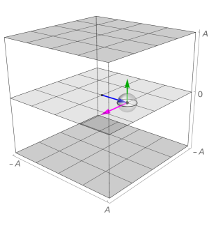
(a)  Single black hole configuration.

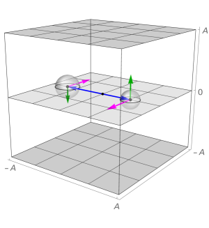
(b)  Binary black hole configuration.

Figure 1: The initial data three-surface $\Sigma$. The initial data surface is represented as a finite cube centered at the origin of $\mathbb{R}^{3}$ with edges of length $2A$ for (a) single and (b) binary black hole configuration.

In the present work, we choose to work with Cartesian coordinates $(x,y,z)$ and to foliate $\Sigma$ with $z=\mathrm{const.}$ two-surfaces. With these choices the constraints (II.4)-(II.6) for the fields $(\widehat{N},{\bf k}_{A},{\bf K})$ take respectively the form

$$\partial_{z}\widehat{N}=A_{1}\,\partial^{2}_{xx}\widehat{N}+A_{2}\,\partial^{2}_{yy}\widehat{N}+A_{3}\,\partial^{2}_{xy}\widehat{N}+A_{4}\,\partial_{x}\widehat{N}+A_{5}\,\partial_{y}\widehat{N}+\mathcal{A}\,\widehat{N}+\mathcal{B}\,\widehat{N}{}^{3},$$ (II.7)

$$\partial_{z}{\bf k}_{x}=B_{1}\,\partial_{x}{\bf k}_{x}+B_{2}\,\partial_{y}{\bf k}_{x}+B_{3}\,\partial_{x}{\bf K}+B_{4},$$ (II.8)

$$\partial_{z}{\bf k}_{y}=C_{1}\,\partial_{x}{\bf k}_{y}+C_{2}\,\partial_{y}{\bf k}_{y}+C_{3}\,\partial_{y}{\bf K}+C_{4},$$ (II.9)

$$\partial_{z}{\bf K}=D_{1}\,\partial_{x}{\bf K}+D_{2}\,\partial_{y}{\bf K}+D_{3}\,\partial_{x}{\bf k}_{x}+D_{4}\,\partial_{x}{\bf k}_{y}+D_{5}\,\partial_{y}{\bf k}_{x}+D_{6}\,\partial_{y}{\bf k}_{y}+D_{7},$$ (II.10)

where ${\bf k}_{x},{\bf k}_{y}$ are the components of the vector ${\bf k}_{A}$ along the $x,y$ direction, respectively; the functions $\mathcal{A}$ and $\mathcal{B}$ have been defined above; and the exact expressions of the functions $A_{i},B_{i},C_{i},D_{i}$ are given in Appendix A. In Sec. III the above system will be solved numerically for several different black hole configurations.

In the setting of Fig. 1, the considered black holes are placed on the $z=0$ plane and lie along the $y$-axis at distance $\vec{d}^{[i]}=d^{[i]}\hat{e}_{y}$ from the origin with linear velocity $\vec{\upsilon}^{[i]}=\upsilon^{[i]}\hat{e}_{x}$ along the $x$-direction and carry spin $\vec{s}^{[i]}=M^{[i]}a^{[i]}\hat{e}_{z}$ along the $z$-direction. (The unit vectors $\hat{e}_{i}$ are aligned along the respective positive directions.) In order to avoid configurations with extremal black holes or with naked singularities, in the following it will be always assumed that $|a^{[i]}|<M^{[i]}$.

According to Rácz (2018, ), the values of the freely-specifiable fields $(\widehat{N}^{A},\,\widehat{\gamma}_{AB},\,\boldsymbol{\kappa},\,\overset{\circ}{\rm\bf K}_{AB})$ must be prescribed throughout $\Sigma$ and for the remaining three constraint fields $(\widehat{N},\,{\rm\bf k}{}_{A},\,{\bf K})$ the constraints (II.7)-(II.10) must be solved. The latter requires the initialisation of the constraint fields on a $z=\mathrm{const.}$ plane. One can prescribe initial data for the fields $(\widehat{N},\,{\rm\bf k}{}_{A},\,{\bf K})$ on one of the shaded (upper or lower) sides of the cubes in Fig. 1 that are positioned at $z=\pm A$. Then, by solving the constraints (II.7)-(II.10), these data can be evolved along the $z$-streamlines towards the plane at $z=0$ where the black hole singularities are located. In addition, because of the finite nature of $\Sigma$, boundary conditions for the constrained fields must be also prescribed on the four vertical sides of $\Sigma$ located at $x=y=\pm A$.

In order to provide the aforementioned values to the fields $(\widehat{N},\,{\bf k}{}_{A},\,{\bf K};\widehat{N}^{A},\,\widehat{\gamma}_{AB},\,\boldsymbol{\kappa},\,\overset{\circ}{\rm\bf K}_{AB})$, we follow the proposal put forward in Rácz (2018, ). Therein, Kerr-Schild type black hole data are used to provide the values of the constrained fields $(\widehat{N},\,{\rm\bf k}{}_{A},\,{\bf K})$ on the sides of $\Sigma$ and of the freely-specifiable fields $(\widehat{N}^{A},\,\widehat{\gamma}_{AB},\,\boldsymbol{\kappa},\,\overset{\circ}{\bf K}_{AB})$ throughout $\Sigma$. For an exhaustive and extremely detailed discussion of this topic see Rácz (2018, ); Nakonieczna et al. (2017). Here, we just present the form of the space-time metric for a generic boosted and displaced Kerr-Schild black hole

$$g_{\alpha\beta}=\eta_{\alpha\beta}+2\,H\,\ell_{\alpha}\,\ell_{\beta}$$ (II.11)

and for a pair of superposed Kerr-Schild black holes

$$g_{\alpha\beta}=\eta_{\alpha\beta}+2H^{[1]}\,\ell_{\alpha}{}^{[1]}\,\ell_{\beta}{}^{[1]}+2H^{[2]}\,\ell_{\alpha}{}^{[2]}\,\ell_{\beta}{}^{[2]},$$ (II.12)

where, in inertial coordinates $(t,x,y,z)$ adapted to the background Minkowski metric $\eta_{\alpha\beta}$, we have

$$H=\frac{r^{\prime 3}M}{r^{\prime 4}+{a^{2}z^{2}}},\quad\ell_{\alpha}=\left(\gamma-\gamma\,\upsilon\,\ell^{\prime}_{1},-\gamma\,\upsilon+\gamma\,\ell^{\prime}_{1},\ell^{\prime}_{2},\ell^{\prime}_{3}\right)$$

with $\ell^{\prime}_{\alpha}=\left(1,\frac{r^{\prime}\,x^{\prime}+a\,y^{\prime}}{r^{\prime 2}+a^{2}},\frac{r^{\prime}\,y^{\prime}-a\,x^{\prime}}{r^{\prime 2}+a^{2}},\frac{z}{r^{\prime}}\right)$ and $r^{\prime 4}-(x^{\prime 2}+y^{\prime 2}+z^{2}-a^{2})\,r^{\prime 2}-a^{2}\,z^{2}=0$, $x^{\prime}=\gamma\,x-\gamma\,\upsilon\,t,y^{\prime}=y-d$, $\gamma=1/\sqrt{1-\upsilon^{2}}$.

Therefore, in the following, the values of the fields $(\widehat{N}^{A},\,\widehat{\gamma}_{AB},\,\boldsymbol{\kappa},\,\overset{\circ}{\bf K}_{AB})$ throughout $\Sigma$ and of $(\widehat{N},\,{\bf k}_{A},\,{\bf K})$ on the boundaries of $\Sigma$ for single and binary black hole configurations will be deduced from (II.11) and (II.12), respectively. A comment about the use of (II.12) is in order here. It turns out that although the metric (II.12) does not satisfy Einstein’s vacuum equations, it is a very good candidate for our purposes here as it is asymptotically flat and can be used to approximate the regions close to the individual black holes quite well Rácz and Winicour (2015). At first sight, such a proposal seems at least preposterous. A closer look though puts things back in place again as the numerically computed solutions of the constraints (II.7)-(II.10) will always differ from the corresponding fields that could be deduced analytically from the metric (II.12).

III Numerical implementation

III.1 Setting up the numerical scheme

We choose to solve the constraints (II.7)-(II.10) numerically using the so-called Alternating Direction Implicit (ADI) method. An implicit method was preferred over the explicit methods mainly because of its superior stability and convergence features in the treatment of the parabolic PDE (II.7). It can be shown, see e.g. Douglas (1955), that for (II.7) the ADI method is unconditionally stable and second order in the evolutionary coordinate. The unconditional stability of the ADI method will enable us to get as close as possible to the $z=0$ plane where the black holes singularities are located. Moreover, the ADI method was preferred over the Crank-Nicolson implicit method because the use of the latter for two-dimensional parabolic PDEs like (II.7) becomes essentially impractical due to the high complexity involved.

We use the method of lines to discretize the $1+2$ parabolic-hyperbolic system (II.7)-(II.10). Accordingly, the latter will be reduced to a system of ordinary differential equations by discretizing the spatial coordinates $(x,y)$ with finite difference techniques. In accordance with the setting of Sec. II.2, our two-dimensional computational domain is $(x,y)\in D=[-A,A]\times[-A,A]$, where $2A$ is the length of the edges of the cubes of Fig. 1. To obtain a finite representation of $D$ an equidistant two-dimensional grid $(x_{i},y_{j})=(-A+i\,h_{x},-A+j\,h_{y})$ with grid spacings $(h_{x},h_{y})=(2A/N_{x},2A/N_{y})$ is introduced, where $i=0,\dots,N_{x}$, $j=0,\dots,N_{y}$ with $N_{x}+1,N_{y}+1$ being the number of grid-points along the $x,y$-direction, respectively. Notice that in the following, it will be always assumed that $N_{x}=N_{y}$, this is a requirement that is imposed by the ADI method. Each of the fields $\mathbb{F}_{A}=(\widehat{N},\,\widehat{N}^{i},\,\widehat{\gamma}_{ij},\,\boldsymbol{\kappa},\,{\bf k}{}_{i},\,{\bf K},\,\overset{\circ}{\bf K}_{ij})$ is discretised in a similar fashion, i.e. $(\mathbb{F}_{A})_{ij}=\mathbb{F}_{A}(x_{i},y_{j})$.

Next, the spatial derivatives of the constraint fields are approximated with appropriate finite difference operators. As the ADI method is second order accurate in the spatial coordinates, we accordingly choose to use second order central difference operators to approximate the first and second derivatives appearing in (II.7)-(II.10).

The resulting semi-discrete system of ordinary differential equations will be evolved along the $z$-direction with the operator splitting ADI method introduced above. Remember that in the setting of Fig. 1, $z$ is the “dynamical” coordinate along which evolution takes place.

Now, in order to check the convergence of our numerical solutions, we define the convergence rate as follows

$$\mathrm{CR}=\frac{\log_{2}(E_{0}/E_{1})}{\log_{2}(h_{0}/h_{1})},$$ (III.1)

where $E_{0}$ and $E_{1}$ are the normalised $l^{2}$–norms of the errors of the numerical solutions $\mathcal{N}_{0}$ and $\mathcal{N}_{1}$ with resolution $h_{0}$ and $h_{1}$($<h_{0}$), respectively. The normalised $l^{2}$–norms $E_{i}$ will be computed with respect to the available exact solution $\mathcal{E}$, i.e.

$$E_{i}=\frac{1}{N+1}\sqrt{\sum_{k=1}^{N+1}\left|(\mathcal{N}_{i})_{k}-\mathcal{E}_{k}\right|^{2}},$$

or (when an exact solution is not available) with respect to the numerical simulation of the immediate higher resolution:

$$E_{i}=\frac{1}{N+1}\sqrt{\sum_{k=1}^{N+1}\left|(\mathcal{N}_{i})_{k}-(\mathcal{N}_{i+1})_{k}\right|^{2}},$$

where $N+1$ is the number of grid-points along the $x$ or the $y$ direction. (Recall that $N_{x}=N_{y}=N$.)

The code has been written from scratch in Python. A detailed description of the developed implicit numerical scheme and of the technical features of the resulting numerical algorithm will be publish elsewhere.

III.2 Testing the code with exact solutions

Before we start using our code to study numerically the parabolic-hyperbolic system (II.7)-(II.10), we will carry out—as one should always do—some numerical tests to check its performance in real-life scenarios. Known exact black hole solutions are the best candidates for this job. In the following, the developed numerical scheme will be tested in the single black hole case against the well-known Schwarzschild and Kerr solutions and in the binary case against the Brill-Lindquist solution.

III.2.1 Single black holes

Schwarzschild black hole. We start testing the performance of our code with a displaced boosted Schwarzschild black hole expressed in the analytical form (II.11).

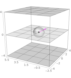
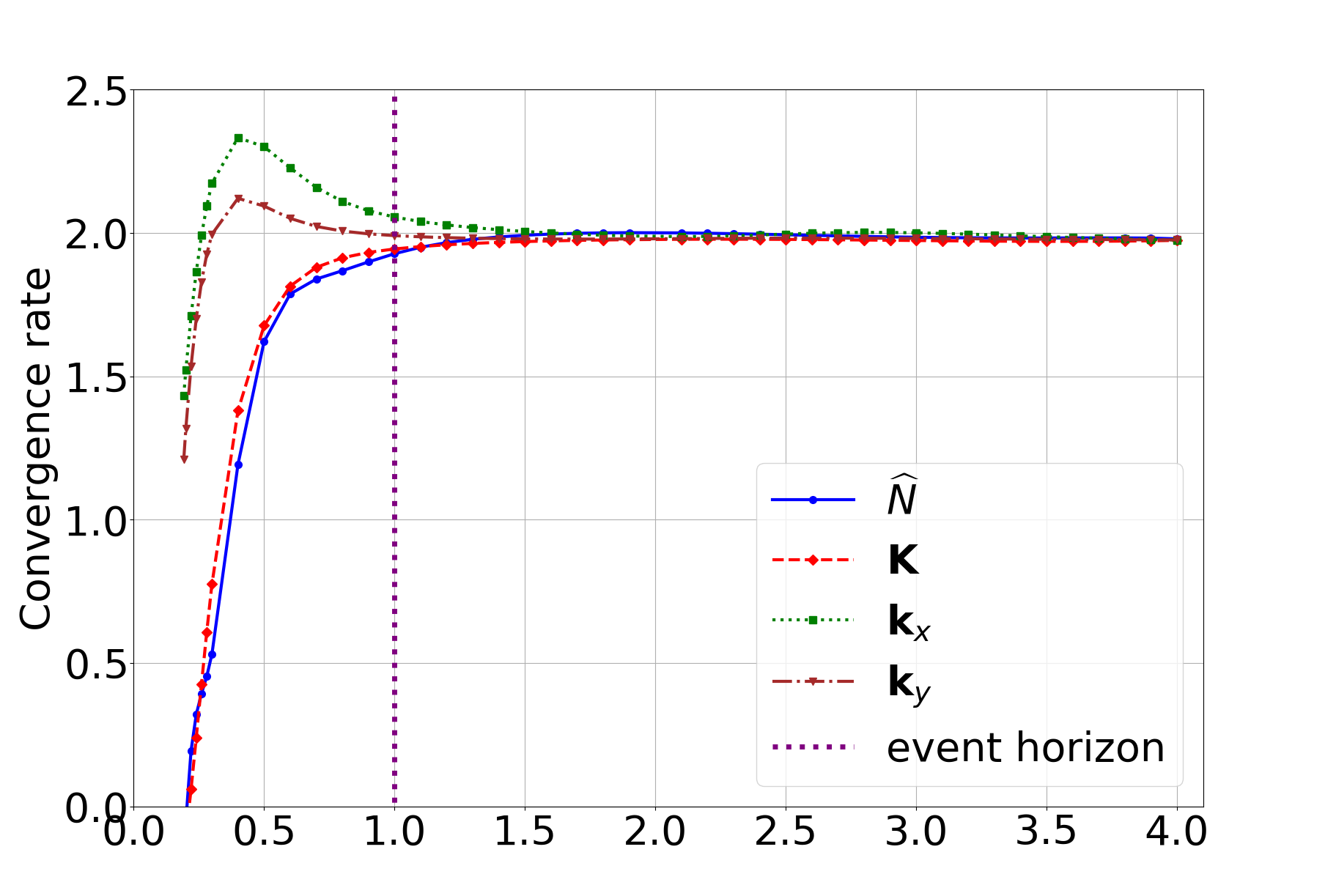
Figure 2: A displaced boosted Schwarzschild black hole. The left panel illustrates the computational domain on which the constraints (II.7)-(II.10) are solved in the case of a Schwarzschild black hole with input parameters $(M,\,d,\,\upsilon)=(0.5,\,1.5,\,0.7)$. The dynamical behaviour of the convergence rate (III.1) for each one of the constrained fields is depicted on the right panel. (Notice the position of the event horizon at $z=1$.)

The input parameters characterising the considered black hole read $(M,\,d,\,\upsilon)=(0.5,\,1.5,\,0.7)$. The left panel of Fig. 2 depicts the location of the black hole, its event horizon, and the direction of its velocity on the computational domain $-4\leq x\leq 4$,  $-2.5\leq y\leq 5.5$,  $0\leq z\leq 4$ used in our numerical simulation. To initialise the $z$-evolution initial data for the constrained fields are prescribed on the upper shaded horizontal side of the cube located at $z=4$. Subsequently, using the constraints (II.7)-(II.10), these initial data are evolved towards the $z=0$ plane where the black hole singularity is located.

The resulting numerical solutions are highly accurate and our findings concerning their convergence properties are presented on the right panel of Fig. 2. Therein, the dynamical behaviour of the convergence rates for each one of the constrained fields is illustrated. It is clearly visible that during most of the evolution the convergence rates of all the constrained fields are around $2$, even when we are quite inside the event horizon. The expected drop of convergence while approaching the $z=0$ plane (where the singularity is located) can be considerable slowed down and delayed by increasing the resolution of our simulations. This quite challenging numerical feature is less alarming than one would expect, as it has been already shown in Nakonieczna et al. (2017), that the accuracy of the produced data and the convergence properties of our numerical scheme close to the $z=0$ plane can be considerably improved by employing the so-called deviation form of the parabolic-hyperbolic system.

Kerr black hole. Next, we test our code with respect to a displaced boosted Kerr black hole given in the analytical form (II.11) with input parameters $(M,\,d,\,\upsilon,\,a)=(0.5,\,2.5,\,0.6,\,0.15)$. Our numerical setting depicted on the left panel of Fig. 3 is quite similar to the one for the Schwarzschild black hole discussed above—this is the first instance of the holistic nature of the new approach. The location of the black hole, the outer event horizon, the direction of the velocity, and the ring singularity of radius $r_{ring}=0.15$—blue ring confined to the $z=0$ plane—are clearly visible on the left panel of Fig. 3. The computational domain used is $-4\leq x\leq 4$,  $-1.5\leq y\leq 6.5$, and $0\leq z\leq 4$.

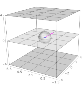
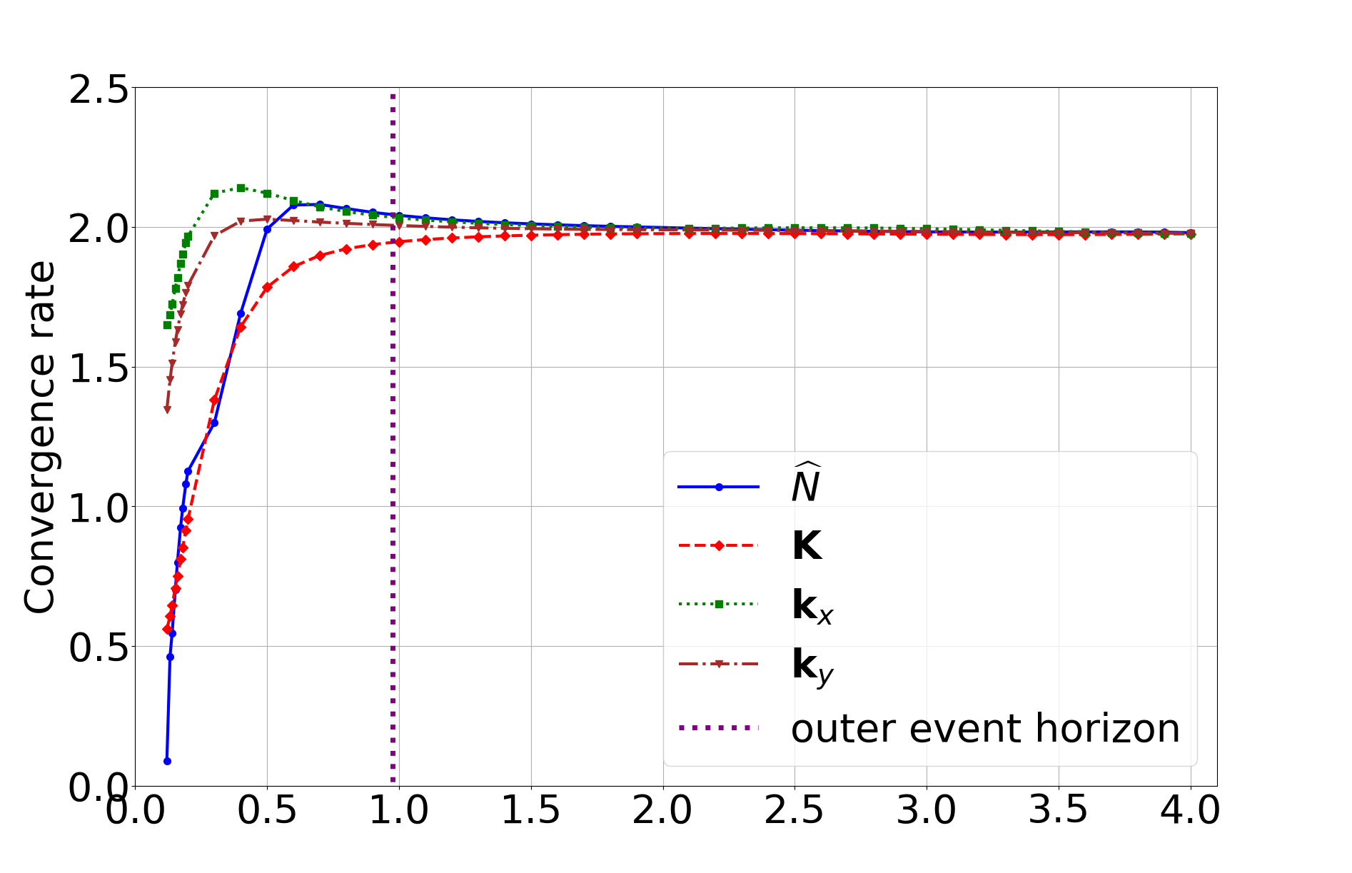
Figure 3: A displaced boosted Kerr black hole. The left panel depicts the computational domain on which initial data for a Kerr black hole with input parameters $(M,\,d,\,\upsilon,\,a)=(0.5,\,2.5,\,0.6,\,0.15)$ are constructed. Notice on the $z=0$ plane the characteristic ring singularity of radius $r_{ring}=0.15$ related to the spin of the black hole. The right panel illustrates the behaviour of the convergence rates of the constrained fields during the $z$-evolution. (Notice that the radius of the outer event horizon is $r_{H}\approx 0.977$.)

The dynamical behaviour of the convergence rate (III.1) for each one of the constrained fields $(\widehat{N},\,{\bf k}_{A},\,{\bf K})$ is illustrated on the right panel of Fig. 3. The convergence rates have been computed with respect to the analytic expressions of the constrained fields deduced from the Kerr-Schild form (II.11) of the considered Kerr black hole. As expected, during the evolution the convergence rates of all the constrained fields range around $2$ and drop gradually as we approach the $z=0$ plane.

III.2.2 Brill-Lindquist binary black holes

The three-metric describing a pair of black holes at a moment of time symmetry is given in Cartesian coordinates by the expression

$$h_{ij}\,dx^{i}dx^{j}=\left(1+\frac{1}{2}\sum_{i=1}^{2}\frac{M^{[i]}}{\left[x^{2}+\left(y-d^{[i]}\right)^{2}+z^{2}\right]}\right)^{4}\left[dx^{2}+dy^{2}+dz^{2}\right],$$ (III.2)

where $M^{[i]}$ and $d^{[i]}$, with $i=1,2$, denote the bare masses and the displacements from the origin, along the $y$-axis, of the two black holes, respectively. (Notice that the Brill-Lindquist metric cannot be written in Kerr-Schild form.) Due to the time-symmetric nature of the Brill-Lindquist data $K_{ij}$ vanishes, therefore all the fields, i.e. $(\boldsymbol{\kappa},\,{\bf k}_{A},\,{\bf K},\,\overset{\circ}{\bf K}_{AB})$, derived from $K_{ij}$ also vanish. Thus, we are left with only two freely-specifiable fields $(\widehat{N}^{A},\,\widehat{\gamma}_{AB})$ and one constrained field $\widehat{N}$. Consequently, we have to solve only the parabolic equation (II.7) for $\widehat{N}$—the rest equations of the parabolic-hyperbolic system (II.7)-(II.10) are trivially satisfied. The initial and boundary values for $\widehat{N}$ and the values of $(\widehat{N}^{A},\,\widehat{\gamma}_{AB})$ throughout $\Sigma$ are deduced from (III.2).

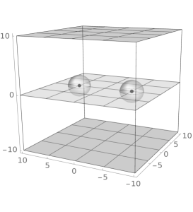
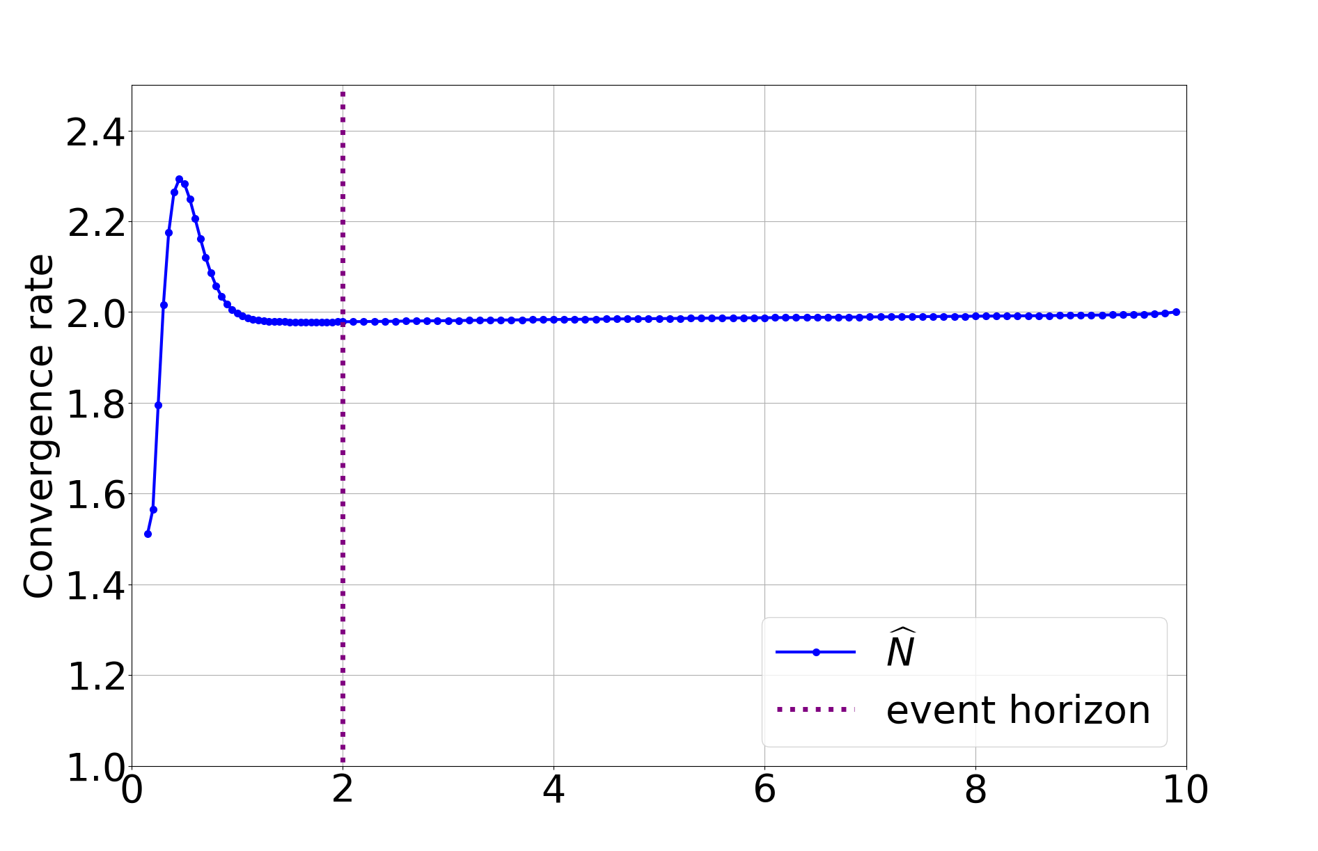
Figure 4: Brill-Lindquist black holes. The two black holes of equal mass $M^{[1]}=M^{[2]}=1$ lie symmetrically to the origin on the $y$-axis with $d^{[1]}=-d^{[2]}=5$. The left panel also depicts the computational domain used in solving the only non-trivially satisfied constraint, i.e. the Hamiltonian constraint (II.7). The dynamical behaviour of the convergence rate of the only non-trivial constraint field $\widehat{N}$ is depicted on the right panel.

The left panel of Fig. 4 depicts our numerical arrangement. A pair of non-boosted black holes with masses $M^{[1]}=M^{[2]}=1$ are positioned on the $y$-axis at distances $d^{[1]}=-d^{[2]}=5$ from the origin. Both black holes are placed on the $z=0$ plane. Our computational domain is $-10\leq x\leq 10,\,-10\leq y\leq 10$, and $0\leq z\leq 10$. Initial data for $\widehat{N}$ are prescribed on the upper shaded horizontal side of the cube located at $z=10$ and are evolved with (II.7) towards the $z=0$ plane where the black hole singularities are positioned.

The behaviour of the convergence rate (III.1) with $z$ of the only non-trivial constrained field $\widehat{N}$ is depicted on the right panel of Fig. 4. The convergence rates during the evolution are around $2$, even on $z$-slices well inside the event horizon, and they only start dropping extremely close to the $z=0$ plane.

III.3 Numerical results: Dynamical black hole configurations

The results of the previous section constitute strong evidence that our code can successfully reproduce the exact single and binary black hole solutions considered in Sec. III.2. Our findings confirm the expected convergence and stability features of the implicit method we are using. Therefore, we are confident enough to proceed further in the numerical investigation of the parabolic-hyperbolic form of the constraints and look for more general non-stationary solutions of the system (II.7)-(II.10).

III.3.1 Distorted Kerr

First, we look for dynamical single black hole solutions of the system (II.7)-(II.10). Specifically, we construct initial data for dynamical single black hole configurations resulting from the distortion of the stationary Kerr black hole considered in Sec. III.2.1.

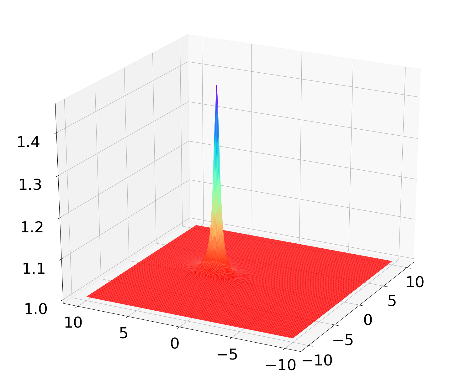
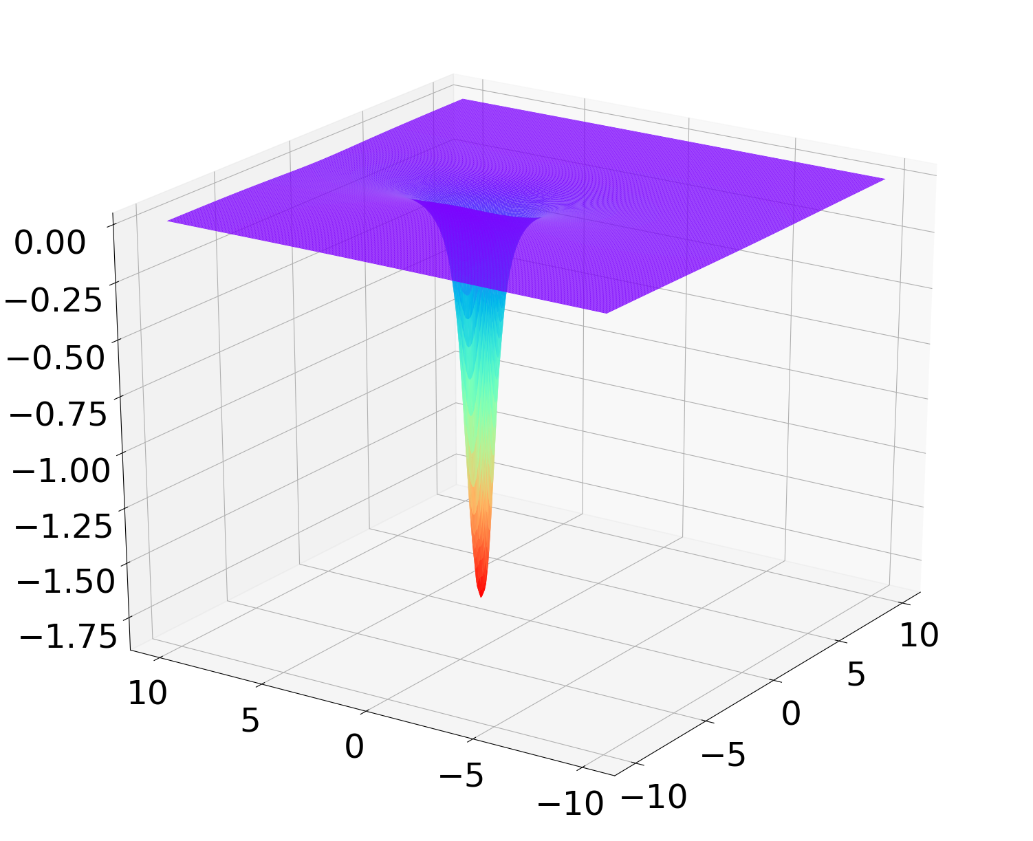
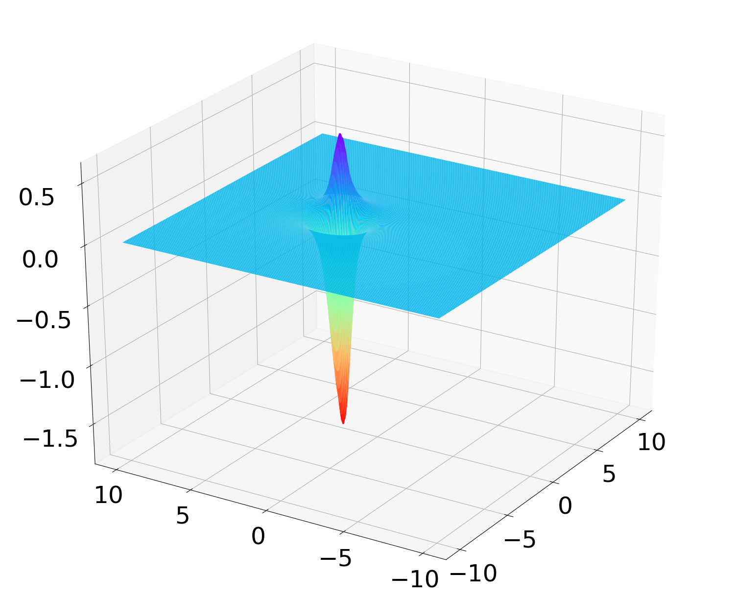
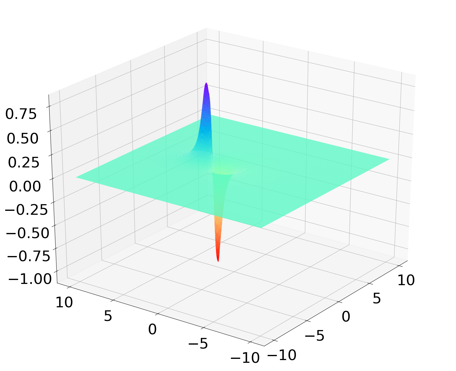
Figure 5: A distorted Kerr black hole. The form of the constrained fields $(\widehat{N},{\bf K},{\bf k}_{x},{\bf k}_{y})$ is depicted at $z=0.5$ resulting from the numerical solution of the constraints (II.7)-(II.10) for the distorted Kerr black hole with input parameters $(M,\,d,\,\upsilon,\,a)=(0.5,\,2.5,\,0.6,\,0.15)$ and $a^{\prime}=0.45$ discussed in the present section.

These are initial data for a dynamical space-time corresponding to a Kerr black hole plus non-trivial gravitational radiation Alcubierre (2008). This kind of non-stationary radiative Kerr black holes can be generated by just altering the Kerr-Schild data used to prescribe initial and boundary conditions to the constrained fields from the Kerr-Schild data used to specify the values of the freely-specifiable fields throughout $\Sigma$.

In principle, any modification of the parameters $M,d,\upsilon,a$ of the Kerr-Schild data can lead to distorted black hole configurations. Here, we choose to alter only the spin. Therefore, we choose the spin of the Kerr-Schild data used to prescribe the initial and boundary values of $(\widehat{N},\,{\bf k}_{A},\,{\bf K})$ to be three times bigger than the spin of the Kerr-Schild data used to specify the values of ($\widehat{N}^{A},\,\widehat{\gamma}_{AB},\,\boldsymbol{\kappa},\,\overset{\circ}{\bf K}_{AB})$ throughout $\Sigma$, i.e. $a^{\prime}=3\,a$. Our numerical setting is similar to the one depicted on the left panel of Fig. 3, namely a black hole of mass $M=0.5$ is placed on the $y$-axis at distance $d=2.5$ from the origin, moves along the $x$-axis with velocity $\upsilon=0.6$, and carries spin $a=0.15$ along the $z$-axis. The computational domain is the same as in the stationary case, i.e. $-4\leq x\leq 4$,  $-1.5\leq y\leq 6.5$, and $0\leq z\leq 4$.

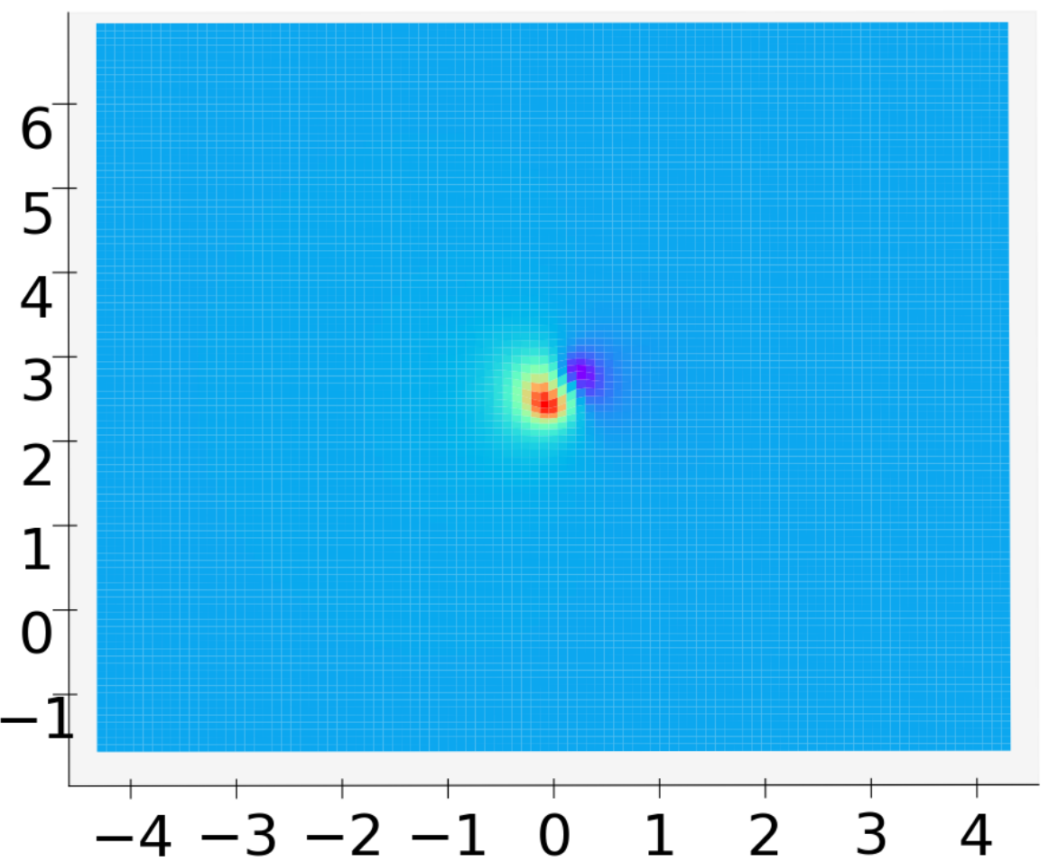
(a)  Stationary ${\bf k}_{x}$

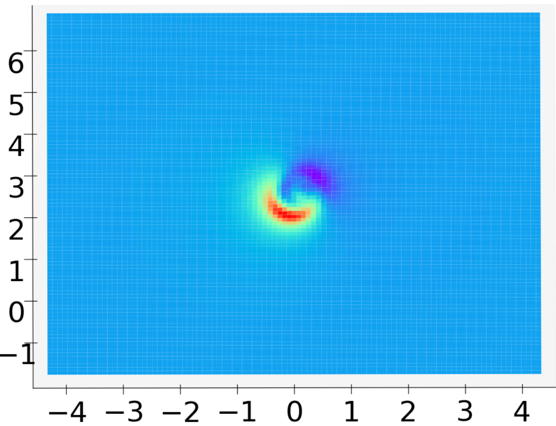
(b)  Distorted ${\bf k}_{x}$

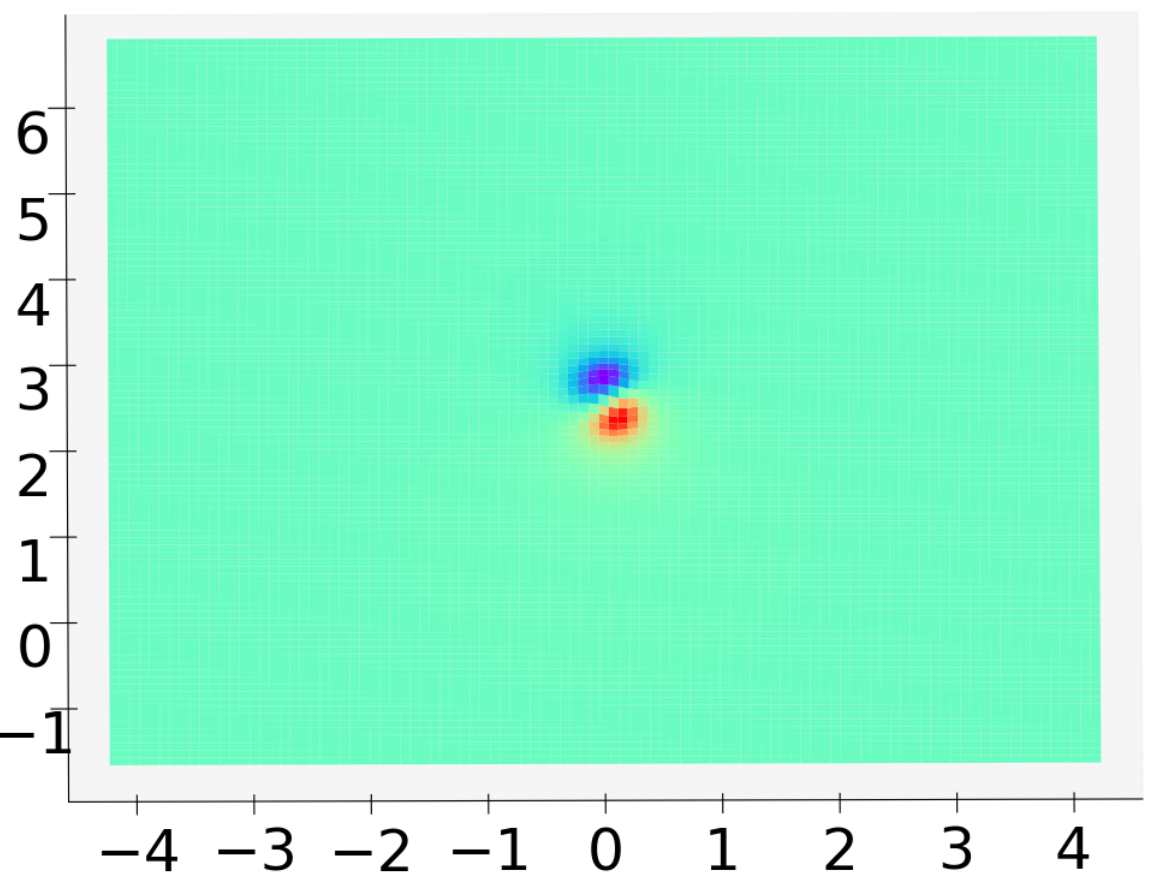
(c)  Stationary ${\bf k}_{y}$

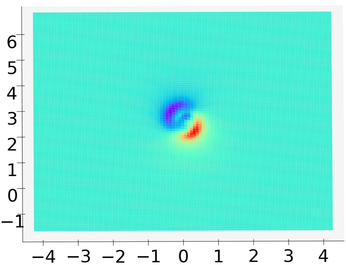
(d)  Distorted ${\bf k}_{y}$

Figure 6: Comparison of the stationary and distorted Kerr black holes considered in the present work. The left and right panels depict the components of the constraint field ${\bf k}_{A}$ for the stationary and distorted Kerr black holes studied in Sec. III.2.1 and the present section, respectively.

Fig. 5 depicts the constrained fields $(\widehat{N},\,{\bf k}_{A},\,{\bf K})$ resulting from the numerical solution of the system (II.7)-(II.10) for the aforedescribed configuration at $z=0.5$. Notice that based on these numerical values of $(\widehat{N},\,{\bf k}_{A},\,{\bf K})$, the physical quantities $(h_{ij},K_{ij})$ can be reconstructed directly from the expressions (II.3).

The left and right panels of Fig. 6 depict the components of the constrained field ${\bf k}_{A}$ for the stationary and distorted Kerr solution considered in Sec. III.2.1 and the present section, respectively. From them it can be safely concluded that the distorted solution of Fig. 5 departs from the stationary solution obtained in Sec. III.2.1. The effect of using larger spin, i.e. $a^{\prime}=3a$, to prescribe the initial and boundary conditions of $(\widehat{N},\,{\bf k}_{A},\,{\bf K})$ is clearly visible on the graphs of the distorted ${\bf k}_{A}$, see right panels of Fig. 6.

We turn now to the convergence analysis of our numerical solution. In contrast to Sec. III.2, here we do not have an exact solution to compare our numerical results with. Therefore, we have to proceed in accordance with the discussion below (III.1) at the end of Sec. III.1. Accordingly, the dynamical behaviour of the convergence rate (III.1) for each of the constraints fields is depicted in Fig. 7. It is apparent that the convergence rates of all the constrained fields are around $2$ for most of the evolution and drop gradually, as expected, the closer we get to the $z=0$ plane.

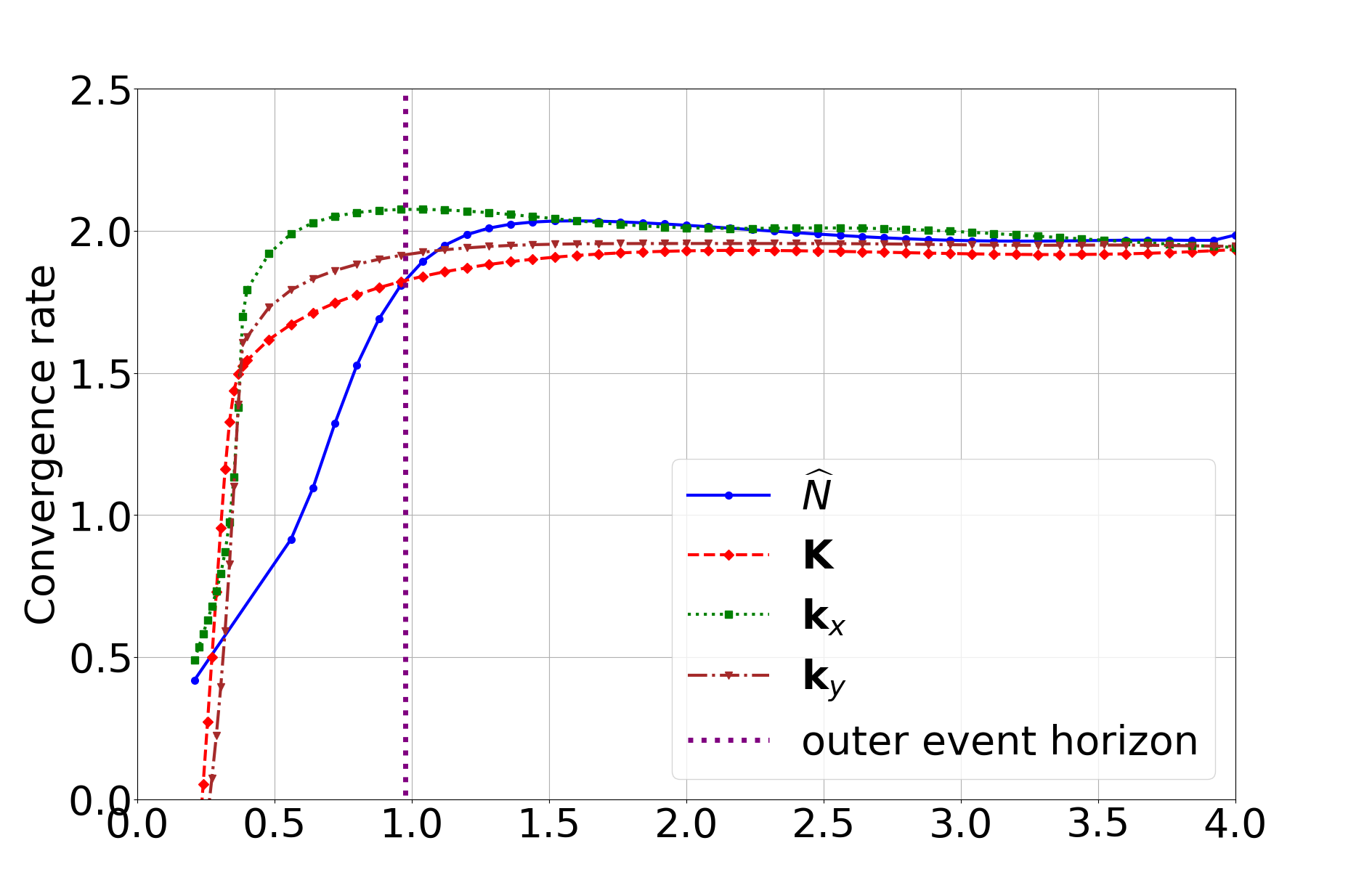
Figure 7: Convergence rates of the constraint fields. The convergence of each one of the constrained fields is depicted as a function of the “temporal” coordinate $z$. The expected behaviour is observed, namely second order convergence in the regions far from the $z=0$ plane and gradual drop of the convergence rates as the $z=0$ plane is approached. The radius of the outer event horizon of the considered distorted Kerr black hole is $r_{H}\approx 0.977$.

III.3.2 Binary black hole systems

We turn now to the main objective of the present work which is the construction of initial data for binary systems of black holes. The importance of constructing such kind of data in the study of the dynamics of black hole binaries has been already stressed in Sec. I. In the following, we will consider a quite general binary black hole configuration consisting of a pair of boosted Kerr black holes. As it was already discussed in Sec. II.2, the binary nature of these data dictates the use of the superposed Kerr-Schild black hole data (II.12) for prescribing the initial and boundary values of the constrained fields $(\widehat{N},\,{\bf k}_{A},\,{\bf K})$ and the values of the freely-specifiable fields $(\widehat{N}^{A},\,\widehat{\gamma}_{AB},\,\boldsymbol{\kappa},\,\overset{\circ}{\bf K}_{AB})$ throughout $\Sigma$.

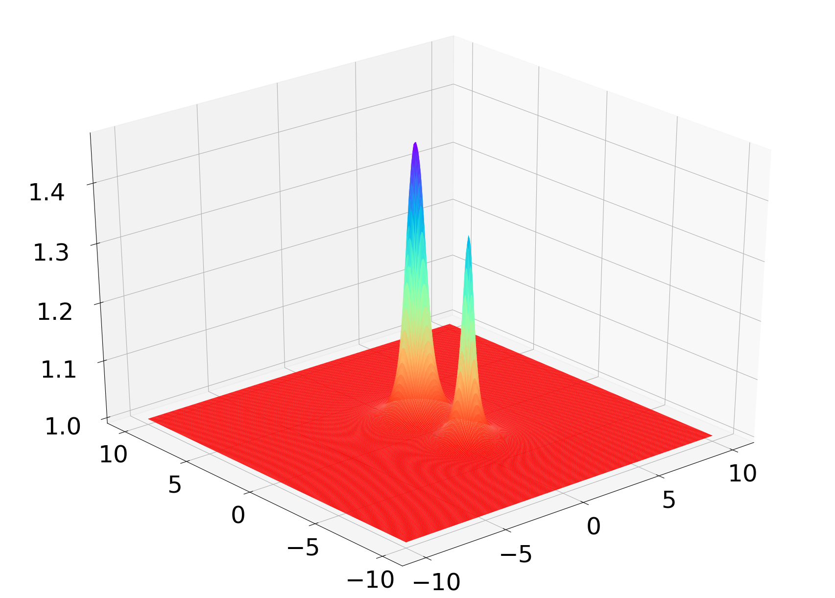
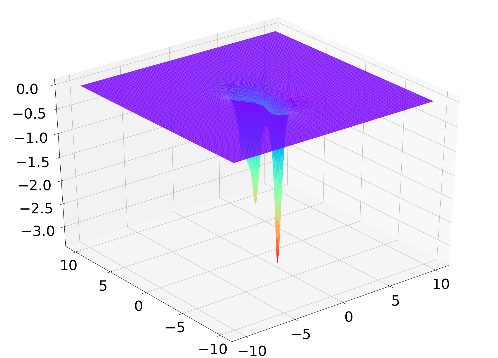
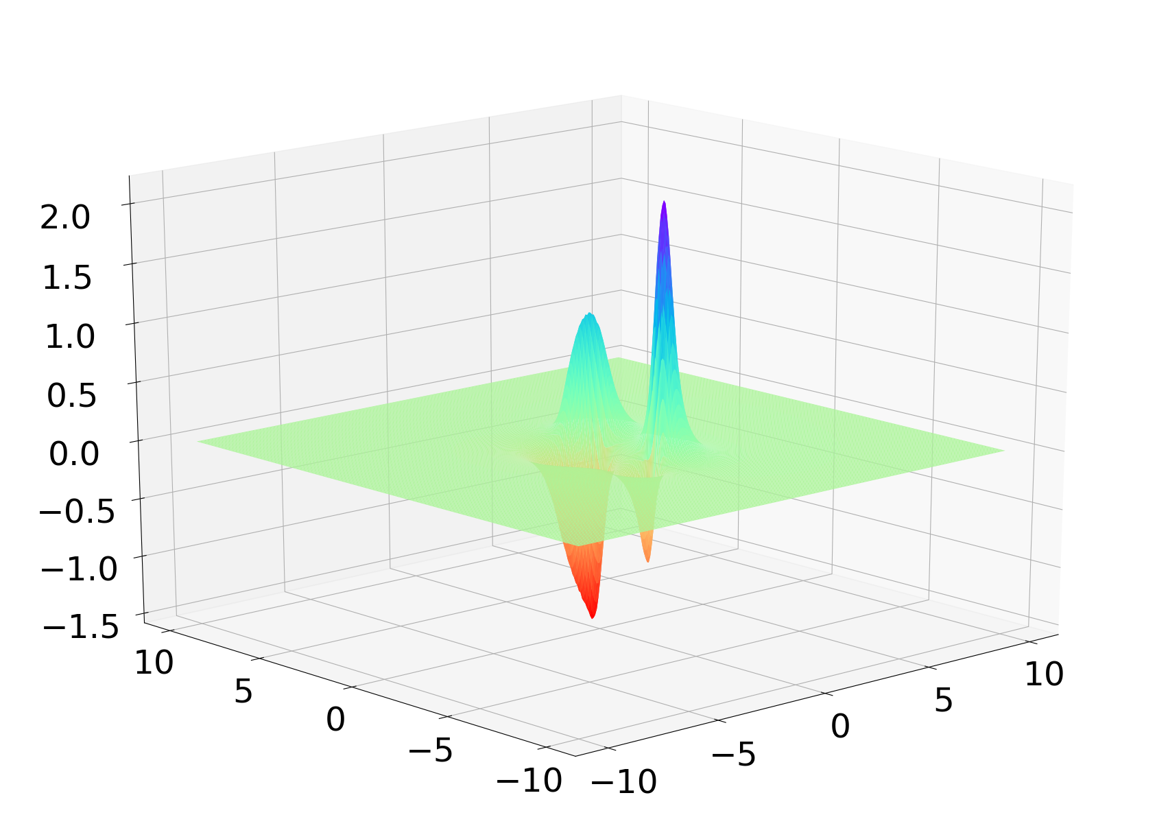
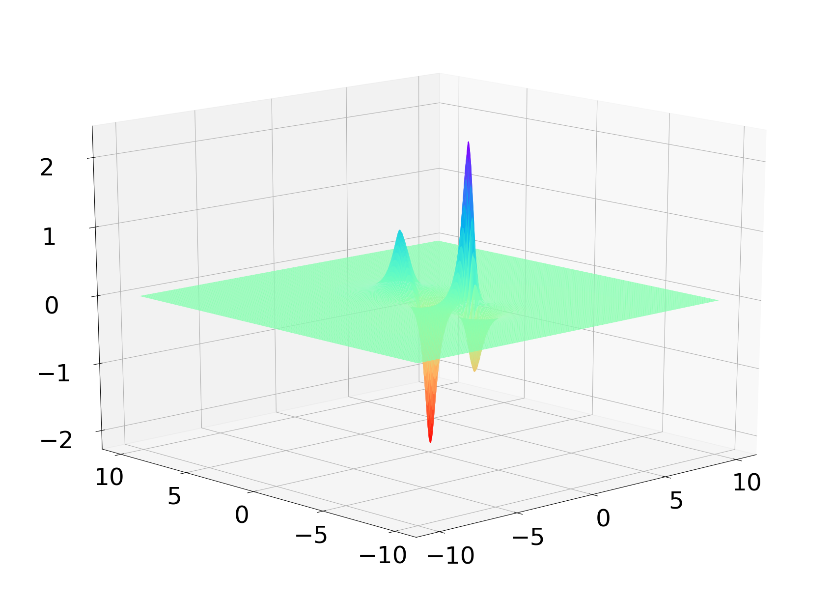
Figure 8: A binary system of two Kerr black holes. The numerically computed constrained fields $(\widehat{N},{\bf K},{\bf k}_{x},{\bf k}_{y})$ are depicted at $z=0.5$ for the binary configuration with input parameters $(M^{[1]},\,d^{[1]},\,\upsilon^{[1]},\,a^{[1]})=(0.72,\,1,\,0.1,\,0.6)$ and $(M^{[2]},\,d^{[2]},\,\upsilon^{[2]},\,a^{[2]})=(0.25,\,-3,\,-0.3,\,-0.2)$.

Our numerical setup consists of two Kerr black holes with masses $M^{[1]}=0.72$ and $M^{[2]}=0.25$ located on the $y$-axis at distance $d^{[1]}=1$ and $d^{[2]}=-3$, respectively, from the origin. The black holes are confined to the $z=0$ plain, move along the $x$-axis with velocities $\upsilon^{[1]}=0.1$ and $\upsilon^{[2]}=-0.3$, and carry anti-parallel spins $a^{[1]}=0.6$ and $a^{[2]}=-0.2$ along the $z$-axis. This setting is similar to the one depicted in Fig. 1(b). Note that the input parameters have been chosen in such a way that the total ADM centre of mass and linear momentum of the binary system are zero, see Rácz (2018). The computational domain is $-10\leq x\leq 10$, $-10\leq y\leq 10$ and $0<z\leq 10$.

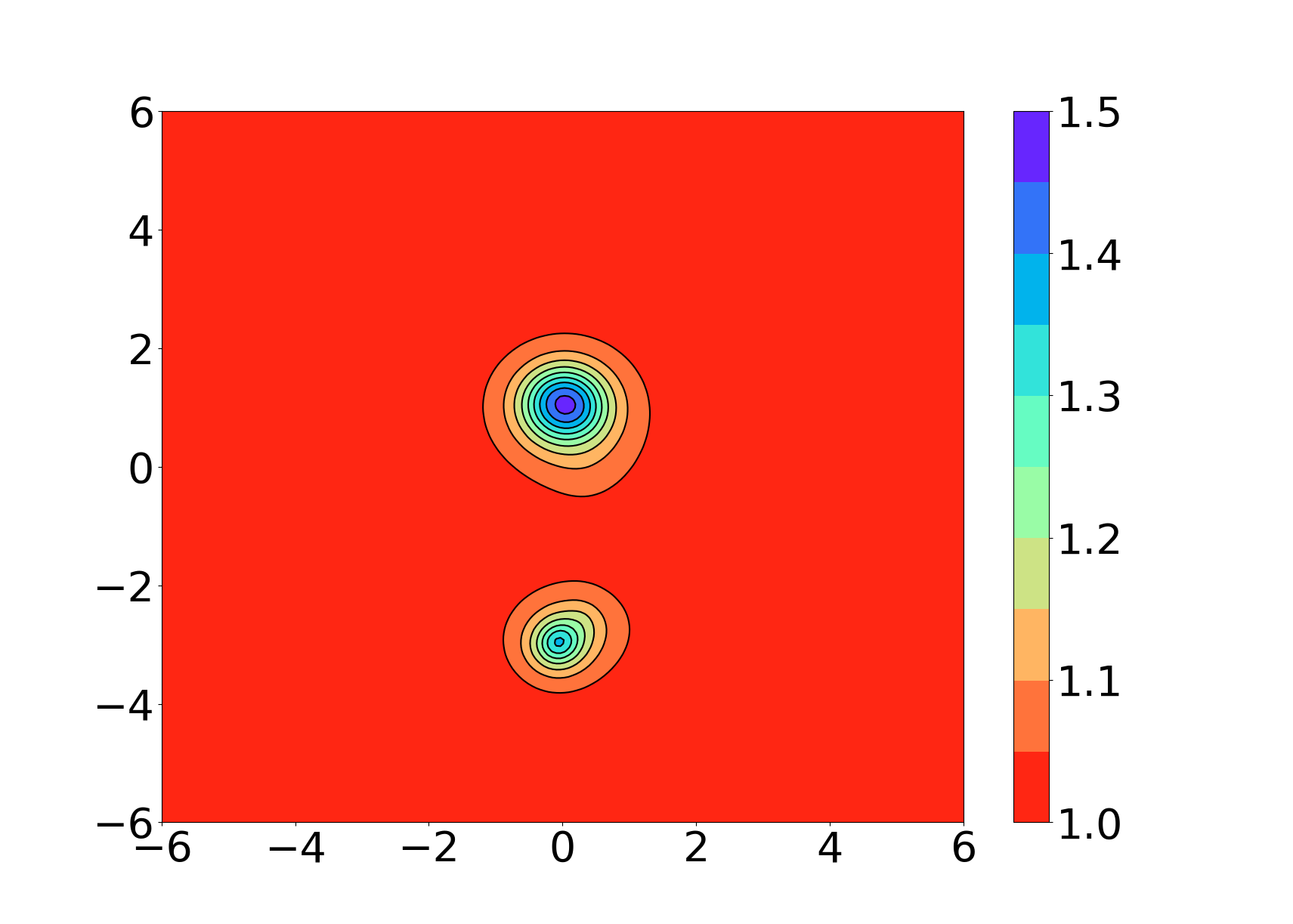
(a)  General case.

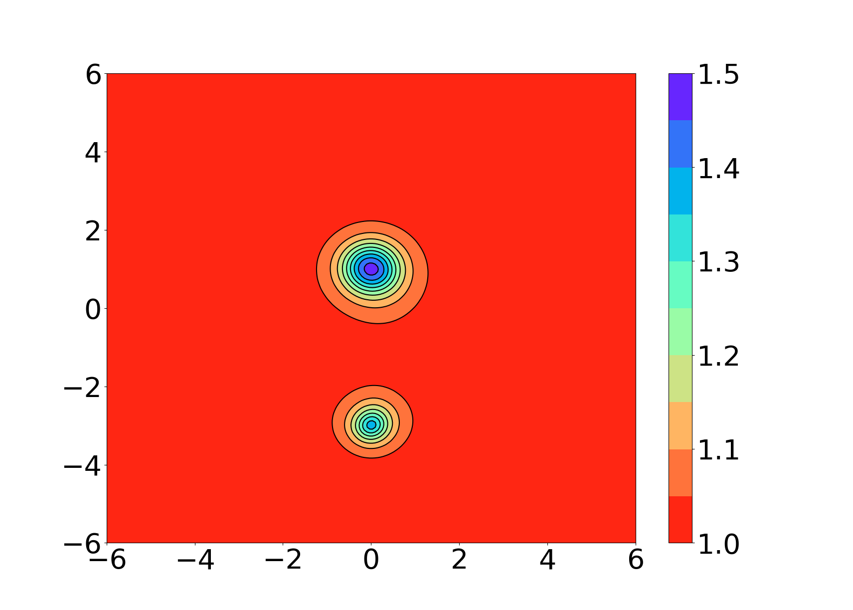
(b)  $\upsilon^{[1]}=\upsilon^{[2]}=0$.

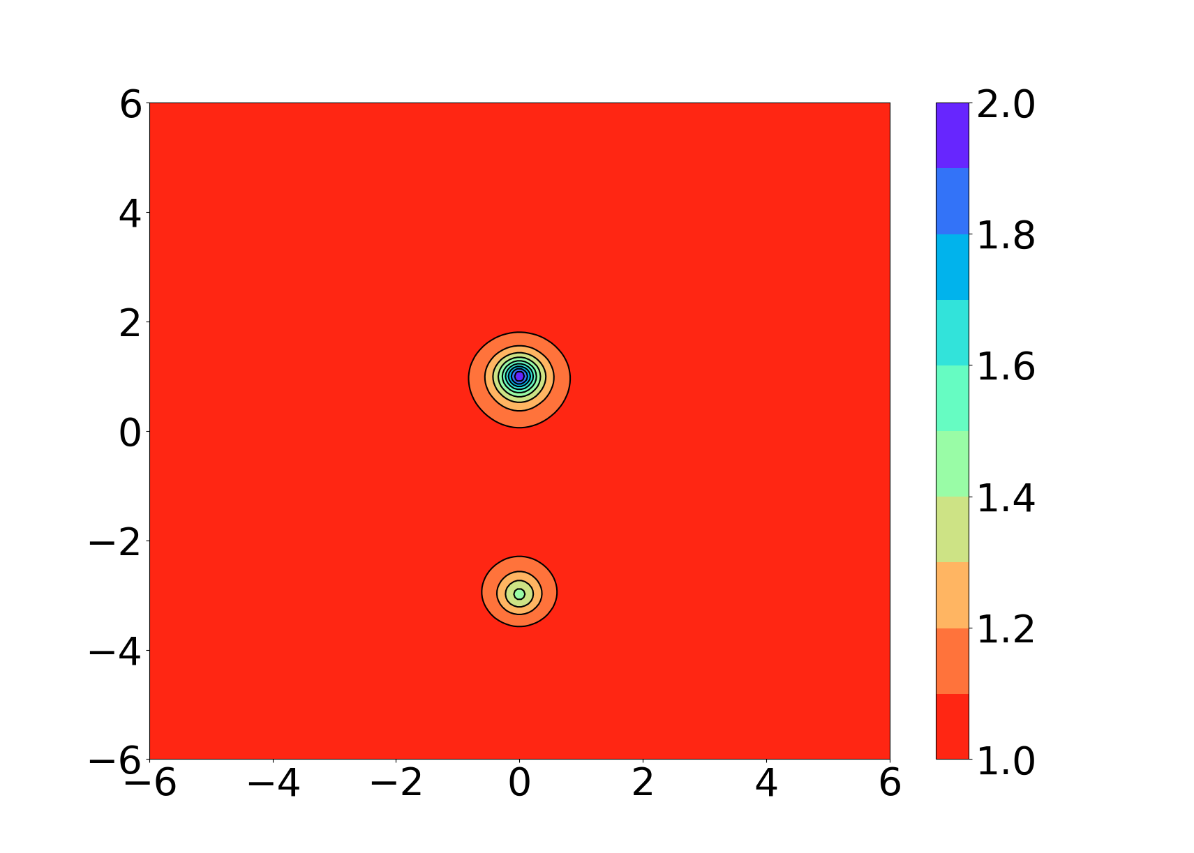
(c)  $a^{[1]}=a^{[2]}=0=\upsilon^{[1]}=\upsilon^{[2]}$.

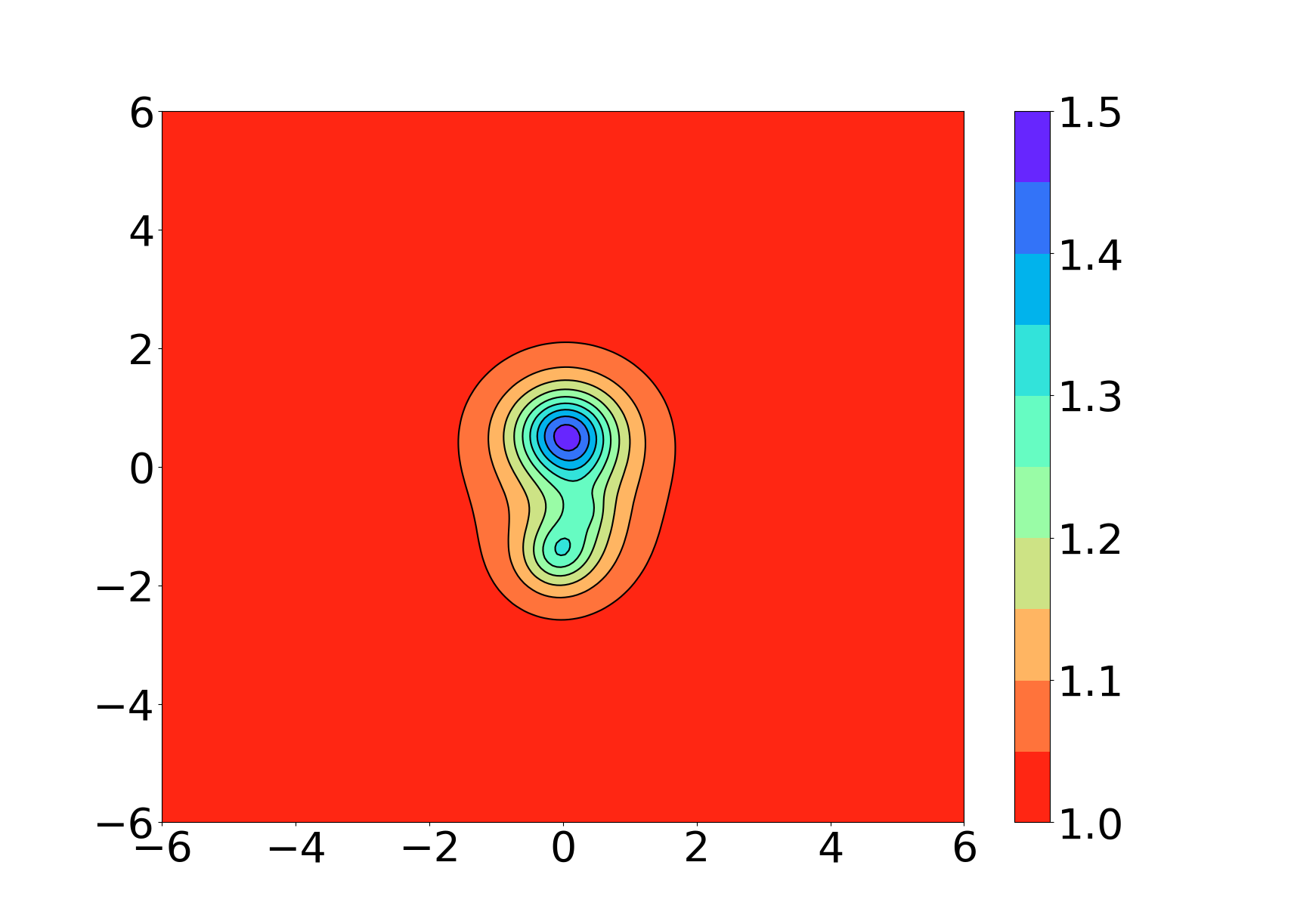
(d)  $d^{\prime[1]}<d^{[1]}$, $d^{\prime[2]}<d^{[2]}$.

Figure 9: Contour plots of the field $\widehat{N}$ for different values of the input parameters of the binary system considered in the present section. Notice that the expected behaviour of the field $\widehat{N}$, under the considered changes of the input parameters, is successfully reproduced by our code.

The form of the numerically computed constrained fields $(\widehat{N},{\bf K},{\bf k}_{x},{\bf k}_{y})$ resulting from the solution of the constraints (II.7)-(II.10) at $z=0.5$ is depicted in Fig. 8. Notice that for the above choice of black hole masses and spins, the radii of their respective outer event horizons are equal to $r_{H}^{[1]}\approx 1.115$ and $r_{H}^{[2]}=0.4$. Therefore, the $z=0.5$ plain, on which the constrained fields of Fig. 8 have been computed, is well inside the outer event horizon of the more massive black hole but still outside the outer event horizon of the less massive one. The binary nature of the constructed initial data is clearly visible on the plots of the four constrained fields—compare with Fig. 5.

As a first test of our implicit numerical scheme, we will study its behaviour with the change of the input parameters of the considered binary system. As reference we will use the contour plot of the field $\widehat{N}$ at $z=0.5$ depicted in Fig. 9(a). Observe that the contours of the two black holes on this plot are slightly deformed because of their non-vanishing linear velocity. Intuitively, one would expect that when the linear velocities of the black holes vanish, then their contours will acquire a more symmetric shape. Clearly, our numerical findings in the case $\upsilon^{[i]}=0$, depicted in Fig. 9(b), fulfil this expectation. If in addition the spins of the black holes are also set to zero then, as shown in Fig. 9(c), the symmetric shape of the contours is still preserved but their size has decreased significantly because of the lack of spin. Moreover, it is expected that when the distance $d=|d^{[1]}|+|d^{[2]}|$ between the black holes is gradually decreased, then for a specific value of $d$ a third horizon surrounding both black holes will form. The contour plot of Fig. 9(d), illustrating our numerical findings for the configuration $d\,^{\prime}<d$, points to this direction as thereon a new contour surrounding both black holes is clearly visible.

We move on now to the numerical analysis of the solution of Fig. 8. Its basic features are encapsulated in Fig. 10. Therein the dynamical behaviour of the convergence rate (III.1) for each one of the constrained fields is depicted. As expected the convergence rates of all the fields are around $2$ for most of the $z$-evolution and drop gradually as we approach the $z=0$ plain where the black hole singularities are located.

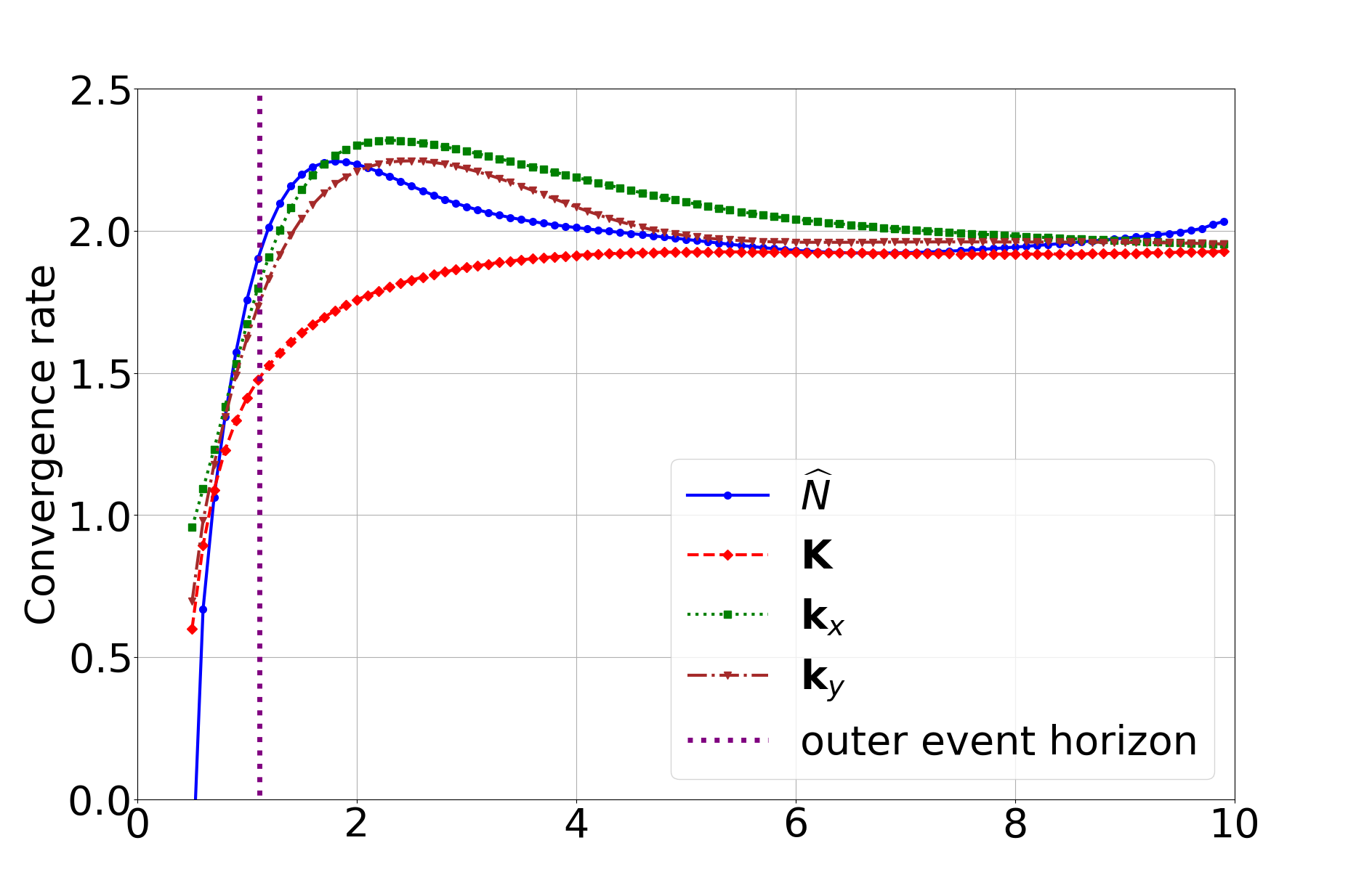
Figure 10: Convergence of the constrained fields. The $z$-dependence of the convergence rate for each one of the constrained fields of the numerical solution depicted in Fig. 8 is shown. The convergence is second order and drops progressively while approaching the $z=0$ plane containing the black hole singularities. Notice that the dashed line depicts the location of the outer event horizon of the more massive black hole with radius $r_{H}\approx 1.115$.

IV Discussion

The purpose of the present paper is to develop an implicit numerical scheme for the parabolic-hyperbolic formulation of the constraints that can be used to construct highly accurate initial data for single and binary black hole configurations.

The above has been achieved by combining the parabolic-hyperbolic formulation of the constraints Rácz (2015) with the superposed Kerr-Schild black hole type data in the way proposed in Rácz (2018, ). In this setting, the constraints are formulated as an initial-boundary value problem for the fields $(\widehat{N},{\bf k}_{i},{\bf K})$ on an initial data three-surface represented as a cube $\Sigma$ of finite side, see Sec II.2. The resulting constraint equations (II.7)-(II.10) are solved on $\Sigma$ given that the values of the freely-specifiable fields $(\widehat{N}^{i},\widehat{\gamma}_{ij},\boldsymbol{\kappa},\accentset{\smash{\raisebox{0.0pt}{$\scriptstyle\circ$}}}{\bf K}\rule{0.0pt}{9.90276pt}_{ij})$ and of the constrained fields $(\widehat{N},{\bf k}_{i},{\bf K})$ have been appropriately provided throughout and on the sides of $\Sigma$, respectively. Kerr-Schild data, briefly discussed in Sec. II.2, are then used to prescribe the initial and boundary values of $(\widehat{N},{\bf k}_{i},{\bf K})$ on the sides of $\Sigma$ and the values of $(\widehat{N}^{i},\widehat{\gamma}_{ij},\boldsymbol{\kappa},\accentset{\smash{\raisebox{0.0pt}{$\scriptstyle\circ$}}}{\bf K}\rule{0.0pt}{9.90276pt}_{ij})$ throughout $\Sigma$.

To solve numerically the constraints in their parabolic-hyperbolic form (II.7)-(II.10), we chose to use the A-stable unconditionally stable alternating direction implicit method described in Sec. III.1. The extensive convergence analysis of Sec. III.2 demonstrates the stability, accuracy and convergence properties of our numerical scheme. The performance of the developed numerical scheme was extensively tested against known exact black hole solutions in the single (Schwarzschild and Kerr) and binary (Brill-Lindquist) case. Our results, both for single and binary black hole configurations, confirm the expected convergence and stability features of the implicit method used.

In Sec. III.3 our implicit scheme was used to generate initial data for dynamical (single and binary) black hole configurations carrying non-trivial gravitational radiation. In the single black hole case, initial data for a distorted Kerr black hole were successfully constructed in Sec. III.3.1. The form of the resulting constrained fields is depicted in Fig. 5. This result is the first manifestation of the control we have over the constructed initial data within Rázc’s method. In contrast to the other existing methods, we have full control over the gravitational radiation content of the constructed non-stationary initial data as its appearance is a result of our conscious choice to alter the spin of the used Kerr-Schild data. In the binary black hole case, initial data for a binary system of Kerr black holes were constructed in Sec. III.3.2. This is a first example of the kind of binary initial data that can be constructed with the proposed implicit numerical scheme. Notice that in order to generate the above data sets no boundary conditions were used in the strong field regime.

The above numerical results demonstrate not only the simplicity of the parabolic-hyperbolic method but also its all inclusive nature as different single and binary black hole configurations can be treated within the same numerical setup. Specifically, the only parameters that have to be changed to get the different black hole initial data constructed in the present work are the input parameters characterising the black holes, i.e. $M_{i},d_{i},\upsilon_{i},a_{i}$.

As demonstrated in Fig. 1, the lack of any boundary conditions in the strong field regime makes the parabolic-hyperbolic method highly attractive as the ”junk radiation” common to all the existing formulations of the constraints could be reduced significantly or even entirely suppressed.

Special attention must be given to the relations (II.3) as they give us direct control of the physical quantities $(h_{ij},K_{ij})$. Notice that the lack of any conformal rescalings in our formulation provides a direct way of reconstructing the original fields $(h_{ij},K_{ij})$ from the ones computed numerically.

In the context of the present implicit approach, a different formulation of the parabolic-hyperbolic system that is based on the deviation from a known Kerr-Schild black hole solution is currently developed. As was already shown in Nakonieczna et al. (2017), this approach will not only increase the accuracy of the produced data and improve the convergence properties of our numerical scheme close to the $z=0$ plane, but will also reduce the computational complexity of the proposed implicit scheme and the required computational resources. In addition, we plan to evolve the constructed initial data in collaboration with other numerical relativity groups that have already fully developed evolutionary codes. The evolution of our data will decidedly answer, among others, the question of whether the constructed initial data are “junk radiation”-free.

Appendix A Coefficients of the constraint equations

Here, we present the full form of the coefficients entering the constraints (II.7)-(II.10).

Coefficients of the parabolic equation (II.7):

$$A_{1}=\widehat{N}^{2}\,\accentset{\smash{\raisebox{0.0pt}{$\scriptstyle\star$}}}{K}\rule{0.0pt}{9.90276pt}{}^{-1}\,\gamma^{xx},\qquad A_{2}=\widehat{N}^{2}\,\accentset{\smash{\raisebox{0.0pt}{$\scriptstyle\star$}}}{K}\rule{0.0pt}{9.90276pt}{}^{-1}\,\gamma^{yy},\qquad A_{3}=2\,\widehat{N}^{2}\,\accentset{\smash{\raisebox{0.0pt}{$\scriptstyle\star$}}}{K}\rule{0.0pt}{9.90276pt}{}^{-1}\,\gamma^{xy},$$

$$A_{4}=\widehat{N}^{x}-\widehat{N}^{2}\,\accentset{\smash{\raisebox{0.0pt}{$\scriptstyle\star$}}}{K}\rule{0.0pt}{9.90276pt}{}^{-1}\,\gamma^{AB}\,\widehat{\Gamma}\,^{x}_{BA},\qquad A_{5}=\widehat{N}^{y}-\widehat{N}^{2}\,\accentset{\smash{\raisebox{0.0pt}{$\scriptstyle\star$}}}{K}\rule{0.0pt}{9.90276pt}{}^{-1}\,\gamma^{AB}\,\widehat{\Gamma}\,^{y}_{BA}.$$

Coefficients of the hyperbolic equation (II.8):

$$\qquad\qquad\qquad B_{1}=\widehat{N}^{x},\qquad B_{2}=\widehat{N}^{y},\qquad B_{3}=\frac{\widehat{N}}{2},$$

$$B_{4} =\left(\partial_{x}\widehat{N}^{x}-\accentset{\smash{\raisebox{0.0pt}{$\scriptstyle\star$}}}{K}\rule{0.0pt}{9.90276pt}\right){\bf k}_{x}-\widehat{N}\,\gamma^{CB}\left(\partial_{B}\overset{\circ}{\bf K}_{Cx}-\widehat{\Gamma}\,^{D}_{BC}\,\overset{\circ}{\bf K}_{Dx}-\widehat{\Gamma}\,^{D}_{Bx}\,\overset{\circ}{\bf K}_{CD}\right)+$$

$$+{\bf k}_{y}\,\partial_{x}\widehat{N}^{y}+\widehat{N}\,\partial_{x}\boldsymbol{\kappa}-\widehat{N}\left(\boldsymbol{\kappa}-\frac{1}{2}\,{\bf K}\right)\dot{\widehat{n}}_{x}+\widehat{N}\,\dot{\widehat{n}}{}^{B}\,\overset{\circ}{\bf K}_{Bx}.$$

Coefficients of the hyperbolic equation (II.9):

$$\qquad\qquad\qquad C_{1}=\widehat{N}^{x},\qquad C_{2}=\widehat{N}^{y},\qquad C_{3}=\frac{\widehat{N}}{2},$$

$$C_{4} =\left(\partial_{y}\widehat{N}^{y}-\accentset{\smash{\raisebox{0.0pt}{$\scriptstyle\star$}}}{K}\rule{0.0pt}{9.90276pt}\right){\bf k}_{y}-\widehat{N}\,\gamma^{CB}\left(\partial_{B}\overset{\circ}{\bf K}_{Cy}-\widehat{\Gamma}\,^{D}_{BC}\,\overset{\circ}{\bf K}_{Dy}-\widehat{\Gamma}\,^{D}_{By}\,\overset{\circ}{\bf K}_{CD}\right)+$$

$$+{\bf k}_{x}\,\partial_{y}\widehat{N}^{x}+\widehat{N}\,\partial_{y}\boldsymbol{\kappa}-\widehat{N}\left(\boldsymbol{\kappa}-\frac{1}{2}\,{\bf K}\right)\dot{\widehat{n}}_{y}+\widehat{N}\,\dot{\widehat{n}}{}^{B}\,\overset{\circ}{\bf K}_{By}.$$

Coefficients of the hyperbolic equation (II.10)

$$D_{1}=\widehat{N}^{x},\qquad D_{2}=\widehat{N}^{y},\qquad D_{3}=\widehat{N}\,\gamma^{xx}\,\partial_{x}{\bf k}_{x},\qquad D_{4}=\widehat{N}\,\gamma^{yx}\,\partial_{x}{\bf k}_{y},$$

$$D_{5}=\widehat{N}\,\gamma^{xy}\,\partial_{y}{\bf k}_{x},\qquad D_{6}=\widehat{N}\,\gamma^{yy}\,\partial_{y}{\bf k}_{y},$$

$$D_{7}=-\frac{\accentset{\smash{\raisebox{0.0pt}{$\scriptstyle\star$}}}{K}\rule{0.0pt}{9.90276pt}}{2}\,{\bf K}-\widehat{N}\,\gamma^{AB}\,\widehat{\Gamma}\,^{C}_{AB}\,{\bf k}_{C}-2\,\widehat{N}\,\dot{\widehat{n}}{}^{A}\,{\bf k}_{A}+\accentset{\smash{\raisebox{0.0pt}{$\scriptstyle\star$}}}{K}\rule{0.0pt}{9.90276pt}\,\boldsymbol{\kappa}-\overset{\circ}{\bf K}_{AB}\,\accentset{\smash{\raisebox{0.0pt}{$\scriptstyle\star$}}}{K}\rule{0.0pt}{9.90276pt}{}^{AB}.$$

All the quantities involved in the above expressions have been defined in Sec. II.1 except of the fields $\widehat{\Gamma}$, which are the Christoffel symbols associated with the two-metric $\widehat{\gamma}_{AB}$.

References

- Collaboration and Collaboration (2016) LIGO Scientific Collaboration and Virgo Collaboration, “GW151226: Observation of gravitational waves from a 22-solar-mass binary black hole coalescence,” Phys. Rev. Lett. 116, 241103 (2016), 1606.04855 .
- Collaboration and Collaboration (2018) LIGO Scientific Collaboration and Virgo Collaboration, GWTC-1: A gravitational-wave transient catalog of compact binary mergers observed by LIGO and Virgo during the first and second observing runs, Tech. Rep. P1800307 (LIGO, 2018) 1811.12907 .
- Pretorius (2005) Frans Pretorius, “Evolution of binary black-hole spacetimes,” Phys. Rev. Lett. 95, 121101 (2005), grqc/0507014 .
- Alcubierre (2008) M. Alcubierre, Introduction to 3+1 numerical relativity, 1st ed. (Oxford University Press, 2008).
- Chu (2014) T. Chu, “Including realistic tidal deformations in binary black-hole initial data,” Phys. Rev. D 89, 064062 (2014), 1310.7900 .
- Rácz (2015) I. Rácz, “Constraints as evolutionary systems,” Class. Quantum Grav. 33, 015014 (2015), 1508.01810 .
- Rácz (2017) I. Rácz, “On the ADM charges of multiple black holes,” Preprint (2017), 1608.02283 .
- Rácz (2018) I. Rácz, “A simple method of constructing binary black hole initial data,” Astronomy Reports 62, 953–958 (2018), 1605.01669 .
- (9) I. Rácz, Supplemental Material (2016), available at http://www.kfki.hu/~iracz/SM-BH-data.pdf.
- Choquet-Bruhat (2009) Y. Choquet-Bruhat, General Relativity and the Einstein Equations, 1st ed. (Oxford University Press Inc., 2009).
- Rácz (2014) I. Rácz, “Cauchy problem as a two-surface based ‘geometrodynamics’,” Class. Quantum Grav. 32, 015006 (2014), 1409.4914 .
- Nakonieczna et al. (2017) A. Nakonieczna, Ł. Nakonieczny, and I. Rácz, “Black hole initial data by numerical integration of the parabolic-hyperbolic form of the constraints,” Preprint (2017), 1712.00607 .
- Rácz and Winicour (2015) I. Rácz and J. Winicour, “Black hole initial data without elliptic equations,” Phys. Rev. D 91, 124013 (2015), 1502.06884 .
- Douglas (1955) J. Douglas, “On the numerical integration of by implicit methods,” J. Soc. Indust. Appl. Math. 3, 42–65 (1955).