Weak-coupling to unitarity crossover in Bose-Fermi mixtures: Mixing-demixing and spontaneous symmetry breaking in trapped systems

Abstract

The usual treatment of a Bose-Fermi mixture relies on weak-coupling Gross-Pitaevskii (GP) and density-functional (DF) Lagrangians, often including the more realistic perturbative Lee-Huang-Yang (LHY) corrections. We suggest analytic non-perturbative beyond-mean-field Bose and Fermi Lagrangians valid along the crossover from weak- to strong-coupling limits of intra-species interactions consistent with the LHY corrections and the strong-coupling (unitarity) limit for small and large scattering lengths $|a|$, respectively, and use these to study the Bose-Fermi mixture. We study numerically mixing-demixing and spontaneous symmetry breaking in Bose-Fermi mixtures in spherically-symmetric and quasi-one-dimensional traps while the intra-species Bose and Fermi interactions are varied from weak-coupling to strong-coupling limits.The LHY correction is appropriate for medium to weak atomic interactions and diverges for stronger interactions (large scattering length $|a|$), whereas the present beyond-mean-field Lagrangian is finite in the unitarity limit ($|a|\to\infty$). We illustrate our results using the Bose-Fermi ⁷Li-⁶Li mixture under a spherically-symmetric and a quasi-one-dimensional trap. The results obtained with the present model for density distribution of the Bose-Fermi mixture along the crossover could be qualitatively different from the usual GP-DF Lagrangian with or without LHY corrections. Specifically, we identified spontaneous symmetry breaking and demixing in the present model not found in the usual model with the same values of the parameters.

I Introduction

Soon after the observation of Bose-Einstein condensates (BEC) in ultra-cold, ultra-dilute, harmonically trapped alkali atom vapors BEC , several groups were able to create and study trapped super-fluid Fermi gas FERMI and Bose-Fermi mixture bfmixture in a laboratory. Of these, a study of trapped super-fluid Bose-Fermi mixture is of interest because of a rich variety of phenomena it can exhibit rmpb ; rmpf . Such study can provide information about different intra- and inter-species interactions acting in this mixture. Phase-separation $-$ a typical feature of binary super-fluids $-$ in mixtures of quantum degenerate gases has been investigated in Bose-Fermi systems Molmer ; as . With the advent of experimental techniques, now it is possible to change the different inter- and intra-species interactions in a super-fluid Bose-Fermi mixture by manipulating an external electromagnetic interaction near a Feshbach resonance fesh . Hence, it is of natural interest to see how the different mixed and demixed phases of a super-fluid Bose-Fermi mixture change as the inter- and intra-species interactions are varied. It is also of interest to see if such phases could spontaneously break the symmetry of the underlying Lagrangian.

In the present paper, we study the mixing-demixing transition in Bose-Fermi super-fluid mixtures in three-dimensional isotropic and quasi-one-dimensional (quasi-1D) harmonic traps as the intra-species Bose and Fermi interactions are increased from weak to strong coupling. The hyperfine spin-1/2 Fermi super-fluid is considered to be in a fully paired (spin-up-down) state as ; Barbut rather than in a spin-polarized single hyperfine state Molmer ; bfmixture . We consider the intra-species interaction for Bose (Fermi) component as repulsive (attractive) which can be changed continuously from the weak-coupling limit to unitarity. The inter-species interaction between the Bose and the Fermi components is considered to be repulsive within the weakly coupling region. The strong-coupling unitary limit, where the gas parameter $x=|a|n^{1/3}\to+\infty$ with $a$ the $s$-wave scattering length, and $n$ the density, has recently drawn a great-deal of attention as it is characterized by universal laws arising from scale invariance. This limit is of great interest in different areas, such as, Bose and Fermi super-fluids univ ; castin ; salomon ; salomon2 ; hulet ; jinF , superconductivity string , string theory asoke , neutron star and Bose bstar stars, and quark-gluon plasma quark , and can be achieved in a laboratory fesh in a Bose-Fermi super-fluid mixture.

The usual mean-field treatment of super-fluid Bose-Fermi mixture as is confined to the weak-coupling limit of Bose and Fermi interactions described by the Gross-Pitaevskii (GP) gross ; rmpb Lagrangian for bosons and the density-functional (DF) rmpf Lagrangian for fermions. As the interaction strength is increased, we need a non-perturbative beyond-mean-field description. Lee, Huang and Yang (LHY) provided a perturbative Lagrangian for bosons LHYb and fermions LHYf . Although the LHY Lagrangian is valid for slightly stronger interactions, it is not appropriate for very strong interactions in the unitarity limit, where it diverges. For this investigation, we proposed minimal analytic forms of Bose and Fermi Lagrangians valid from weak-coupling to unitarity with proper LHY LHYb ; LHYf and unitarity limits without fitting parameter(s). Most of previous suggestions for such crossover functions for both bosons bose ; as and fermions fermi ; as were numerical with fitting parameter(s) and hence did not have the analytic LHY limits. With the present analytic weak-coupling to unitarity crossover functions, we write the dynamical beyond-mean-field equations for the Bose-Fermi system, which we use in this study of Bose-Fermi mixture in spherically-symmetric and quasi-1D traps. For a quasi-1D confinement, we use this beyond-mean-field 3D model rather than a strict 1D model obtained from a quantum mechanical many-body 1D Hamiltonian. Such a strict 1D model has novel properties like fermionization of bosons TG . The nonlinearities of the strict 1D model are also different from the present 3D model. For a large finite transverse trap in the present quasi-1D case, as in experiments, the present 3D model should be appropriate. How the present results will approximate the results of the strict 1D model under infinitely strong transverse trap is an open question beyond the scope of the present study.

In the present study, we find that the density distribution of the Bose-Fermi mixture along the weak- to strong-coupling crossover could be qualitatively different from that obtained employing the usual GP-DF Lagrangian with or without the LHY corrections. For example, we found demixing in the Bose-Fermi mixture obtained using the present model where the GP-DF Lagrangian predicted mixing of the components. We also found spontaneous symmetry breaking in the present model not found in the GP-DF model.

The plan of the paper is as follows. In Sec. II, we present the analytic expressions for energy and chemical potential of uniform Bose and Fermi super-fluids along the weak coupling to unitarity crossover and derive the nonlinear equations to study the mixing-demixing transition and spontaneous symmetry breaking in Bose-Fermi super-fluid mixtures. In Sec. III, we present the numerical results along the weak- to strong-coupling crossover for the Bose-Fermi mixture under spherically-symmetric and quasi-1D traps. We compared our results with those obtained from the usual weak-coupling GP-DF Lagrangian for the Bose-Fermi mixture and found that the present results could be qualitatively different. A summary of our findings is given in Sec. IV.

II Analytical model along the weak to strong coupling crossover

Bose and fully-paired Fermi super-fluids in the weak-coupling limit are well described by mean-field GP gross and DF DF rmpf equations, respectively. These equations for bosons rmpb and fermions as are equivalent to the super-fluid hydrodynamic equations. The Bose and Fermi super-fluids are described by a macroscopic order parameter. In case of bosons, the order parameter is also the single-particle wave function in the Hartree approximation of the many-body dynamics. In case of fermions, the macroscopic order parameter refers to a fully-paired bosonic entity known as Cooper pair lnc . Hence, the macroscopic hydrodynamic description of a Fermi super-fluid is formulated in terms of paired fermions in the form of Cooper pairs lnc and not in terms of single-particle Fermi wave function as . Such a description has led to excellent results for many collective xxx ; collective phenomena in many-fermion super-fluids, such as density density distribution or frequency of oscillation xxx , where a many-body description becomes unmanageable.

The macroscopic behavior of a Bose rmpb or Fermi rmpf super-fluid is governed by the classical Landau LANDAU equations of irrotational hydrodynamics with the velocity field ${\bf v}_{i}=\hbar\nabla S_{i}/2m_{i}$, where $S_{i}$ is the phase of the order parameter $\phi_{i}({{\bf r},t})=\sqrt{n_{i}({\bf r},t)}e^{{\mbox{i}}S_{i}({\bf r},t)}$ where ${\mbox{i}}=\sqrt{-1}$, $n_{i}$ is the density, $m_{i}$ is the mass of the fundamental entity responsible for super-fluidity: a bosonic atom or a Fermi pair. Here $i=B$ stands for bosons and $i=P$ for paired fermions. The continuity equation and the irrotational flow equation in this case, e. g., LANDAU

$$\frac{\partial n_{i}}{\partial t} +\nabla\cdot(n_{i}{\bf v}_{i})=0,$$ (1)

$$m_{i}\frac{\partial{\bf v}_{i}}{\partial t} +\nabla\Big{(}V_{i}+\frac{1}{2}m_{i}v_{i}^{2}-\frac{\hbar^{2}\nabla^{2}\sqrt{n_{i}}}{2m_{i}\sqrt{n_{i}}}+\mu_{i}\Big{)} =0,$$ (2)

are entirely equivalent to the following dynamical equation for the order parameter $\phi_{i}({{\bf r},t})$

$${\mbox{i}}\hbar\frac{\partial\phi_{i}}{\partial t}=\Big{(}-\frac{\hbar^{2}}{2m_{i}}\nabla^{2}+V_{i}+\mu_{i}\Big{)}\phi_{i},$$ (3)

where $V$ is an external potential and $\mu_{i},$ is the bulk chemical potential for the uniform Bose or Fermi gas. The quantum pressure term $-{\hbar^{2}\nabla^{2}\sqrt{n_{i}}}/{2m_{i}\sqrt{n_{i}}}$ was not present in Eq. (2) in the original classical flow equations but were introduced later for an accurate description of the dynamics. This term leads to the proper kinetic energy term in the Galilean invariant as dynamical equation (3). For bosons Eq. (3) is the GP equation. For fermions we can relate the fermion and pair variables by $m_{P}=2m_{F},V_{P}=2V_{F},\mu_{P}=2\mu_{F}$ and Eq. (3) becomes the following equivalent density functional (DF) equation

$${\mbox{i}}\hbar\frac{\partial\phi_{F}}{\partial t}=\Big{(}-\frac{\hbar^{2}}{8m_{F}}\nabla^{2}+V_{F}+\mu_{F}\Big{)}\phi_{F}.$$ (4)

In the strong-coupling regime, the scattering length $a_{i}$ is much larger than all length scales ($|a_{i}|\to\infty$) and consequently, the system shows universal behavior univ ; gior ; castin determined by the density $n_{i}$ independent of the parameter $a_{i}$. Here $i=B$ stands for bosons and $i=F$ for paired fermions. By dimensional arguments, the bulk chemical potential of a uniform Bose or Fermi gas at unitarity is given by as ; rmpf

$$\lim_{|a_{i}|\to\infty}\mu_{i}(n_{i},a_{i})=\frac{\hbar^{2}}{m_{i}}\eta_{i}n_{i}^{2/3},$$ (5)

where $\eta_{i}$ is a universal parameter and $m_{i}$ the mass of an atom.

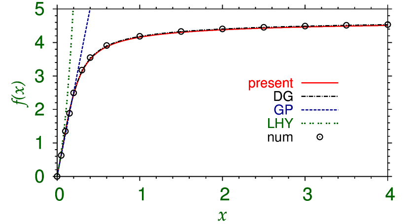
Figure 1: (Color online) Dimensionless function $f(x)$ of the zero-temperature bulk chemical potential (7) versus $x$. present: the crossover function (8) with $\eta_{B}=4.7$, DG: Hartree calculation of Ding and Greene DG , GP: GP function $f(x)=4\pi x$, LHY: LHY function $f(x)=4\pi x+4\pi\alpha x^{5/2}$, num: numerically calculated from energy density (11) using $\mu_{B}=\partial(n_{B}{\cal E}_{B})/\partial n_{B}$.

In the weak-coupling limit the bulk chemical potential of a uniform Bose gas is given by LHYb

$$\mu_{B}(n_{B},a_{B})=\frac{\hbar^{2}}{m_{B}}(4\pi n_{B}a_{B}+2\pi\alpha n_{B}^{3/2}a_{B}^{5/2}+...),$$ (6)

where $\alpha=64/(3\sqrt{\pi}$), and the first term $4\pi n_{B}a_{B}$ on the right-hand side is the weak-coupling mean-field GP gross result and the second term is the perturbative LHY contribution LHYb , which becomes important for moderate values of the scattering length $a_{B}$ $(>0)$. The LHY contribution to $\mu_{B}(n_{B},a_{B})$ has limited validity as it diverges as $a_{B}\to\infty$ at unitarity, whereas the correct $\mu_{B}(n_{B},a_{B})$ should remain finite at unitarity as given by Eq. (5). The minimal analytic form of the non-perturbative bulk chemical potential consistent with the LHY correction (6) and the unitarity limit (5) and also valid along the crossover from weak to strong coupling is scirep

$$\mu_{B}(n_{B},a_{B}) \equiv \frac{\hbar^{2}}{m_{B}}n_{B}^{2/3}f(x),\quad x=a_{B}n_{B}^{1/3},$$ (7)

$$f(x) = 4\pi\frac{x+\alpha x^{5/2}}{1+\frac{\alpha}{2}x^{3/2}+\frac{4\pi\alpha}{\eta_{B}}x^{5/2}}.$$ (8)

Equation (7) with (8) is a Padé approximant to the bulk chemical potential with the proper weak-coupling LHY and unitarity limits. The LHY bosonic energy density consistent with Eq. (6) is

$${\cal E}_{B}(n_{B},a_{B}) \equiv \frac{1}{n_{B}}\int_{0}^{n_{B}}\mu_{i}(n,a_{B})dn$$ (9)

$$= \frac{\hbar^{2}}{m_{B}}\left(2\pi n_{B}a_{B}+\frac{4}{5}\pi\alpha n_{B}^{3/2}a_{B}^{5/2}+...\right).$$

The same at unitarity consistent with Eq. (5) is

$${\cal E}_{B}(n_{B},a_{B})=\frac{\hbar^{2}}{m_{B}}\frac{3}{5}\eta_{B}n_{B}^{2/3}.$$ (10)

These two limiting values can be combined to give the following minimal energy density valid from weak coupling to unitarity

$${\cal E}_{B}(n_{B},a_{B}) \equiv \frac{\hbar^{2}}{m_{B}}\frac{2\pi n_{B}^{2/3}(x+\frac{4\alpha}{5}x^{5/2})}{1+\frac{2\alpha}{5}x^{3/2}+\frac{8\pi\alpha}{3\eta_{B}}x^{5/2}}$$ (11)

Although there is no experimental estimate of the parameter $\eta_{B}$ for bosons despite some attempts univ , there are several microscopic many-body calculations of this parameter lying in the range from 3 to 9 otherB ; DG . Of these, Ding and Greene (DG) DG performed a microscopic Hartree calculation along the crossover and in addition to the value of $\eta_{B}=4.7$, they provided a reliable estimate of the universal function $f(x)$ along the crossover. In Fig. 1, we illustrate the present universal function $f(x)$ of Eq. (8) for $\eta_{B}=4.7$ and compare with the same from the microscopic calculation of DG DG and also with the GP functional $f(x)=4\pi x$ and the LHY functional $f(x)=4\pi(x+\alpha x^{5/2}/2)$. For very small $x$ or for small values $a_{B}$, both the GP and LHY functionals are in reasonable agreement with the present crossover functional as can be seen in Fig. 1. However, for larger $x$, near unitarity, the GP and the LHY contribution cannot describe the actual state of affairs.

For a fully-paired uniform super-fluid of spin-1/2 Fermi gas, the energy density is given by rmpf ; LHYf

$${\cal E}_{F}(n_{F},a_{F}) =\frac{3}{5}E_{F}\left[1+c_{1}y+c_{2}y^{2}+...\right],$$ (12)

$$c_{1} =\frac{10}{9\pi},\quad c_{2}=\frac{4(11-\mbox{ln}4)}{21\pi^{2}},\quad y=k_{F}a_{F},$$ (13)

with Fermi momentum $k_{F}=(3\pi^{2}n_{F})^{1/3}$, Fermi energy $E_{F}=\hbar^{2}k_{F}^{2}/2m_{F}$, $a_{F}$ $(<0)$ the scattering length of spin up-down fermions. In Eq. (12), the first term $3E_{F}/5$ is the DF term as ; rmpf valid in the Bardeen-Cooper-Schrieffer (BCS) bcs weak-coupling limit. The next two terms represent the perturbative LHY contribution LHYf . The energy density at unitarity is written as xxx ; as

$$\lim_{|a_{F}|\to\infty}{\cal E}_{F}(n_{F},a_{F})=\frac{3}{5}E_{F}\eta_{F}.$$ (14)

The minimal analytic energy density along the weak-coupling to unitarity crossover consistent with the weak-coupling LHY limit (12) and the unitarity limit (14) is:

$${\cal E}_{F}(n_{F},a_{F})=\frac{3}{5}E_{F}\left[1+\frac{c_{1}y+(c_{2}-2c_{1}^{2})y^{2}}{1-2c_{1}y+\frac{(c_{2}-2c_{1}^{2})y^{2}}{\eta_{F}-1}}\right].$$ (15)

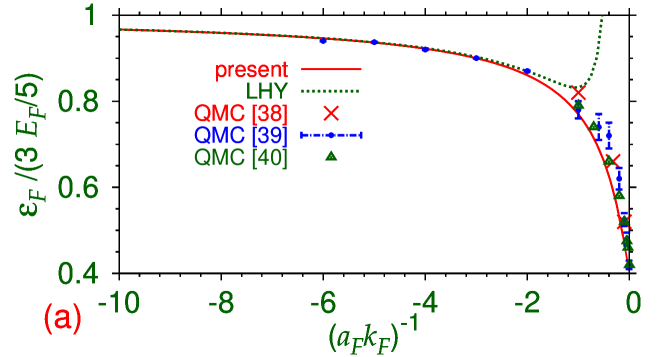
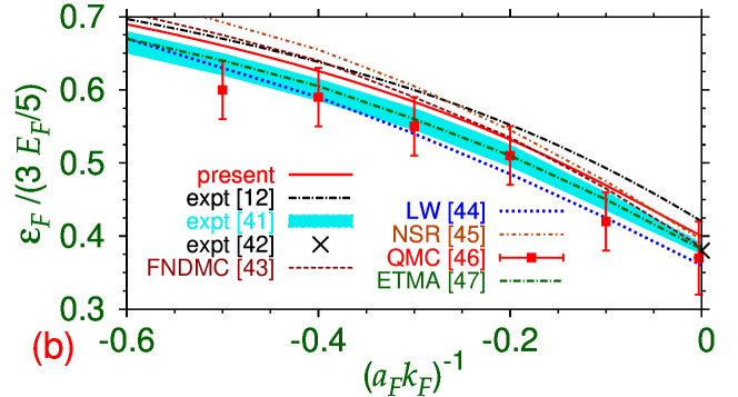
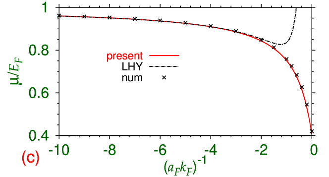
Figure 2: (Color online) Energy density ${\cal E}_{F}$ versus $(a_{F}k_{F})^{-1}$ along the weak-coupling BCS to unitarity crossover: (a) Eq. (15) (present) with $\eta_{F}=0.4$; Eq. (12) (LHY); quantum Monte Carlo results of Ref. microF2 ; Ref. microF1 ; and Ref. microF3 . (b) Eq. (15) (present) with $\eta_{F}=0.4$; experimental results of Refs. salomon , prx , and ku , and theoretical results using FNDMC FNDMC , LW LW , NSR NSR , QMC QMC , and ETMA ETMA methods. (c) Bulk chemical potential $\mu_{F}$ versus $(a_{F}k_{F})^{-1}$ along the weak-coupling BCS to unitarity crossover: Eq. (18) (present) with $\eta_{F}=0.4$; Eq. (16) (LHY); numerically calculated from Eq. (15) using $\mu_{F}=\partial(n_{F}{\cal E}_{F})/\partial n_{F}$ (num).

The following expression for the bulk chemical potential of a uniform Fermi gas in the weak-coupling LHY limit can be obtained from Eq. (12):

$${\cal\mu}_{F}(n_{F},a_{F}) \equiv\frac{\partial(n_{F}{\cal E}_{F})}{\partial n_{F}}=E_{F}\left[1+d_{1}y+d_{2}y^{2}+...\right],$$ (16)

$$d_{1} =\frac{4}{3\pi},\quad d_{2}=\frac{4(11-\mbox{ln}4)}{15\pi^{2}}.$$ (17)

A non-perturbative expression for the chemical potential along the crossover is written in an analogous fashion

$${\cal\mu}_{F}(n_{F},a_{F})\equiv E_{F}g(y),$$ (18)

$$g(y)= \left[1+\frac{d_{1}y+(d_{2}-2d_{1}^{2})y^{2}}{1-2d_{1}y+\frac{(d_{2}-2d_{1}^{2})y^{2}}{\eta_{F}-1}}\right].$$ (19)

This bulk chemical potential has the correct LHY limit (16) and the unitarity limit:

$$\lim_{|a_{F}|\to\infty}{\mu}_{F}(n_{F},a_{F})=E_{F}.$$ (20)

In this paper we will use Eq. (4) to describe Fermi dynamics with $\mu_{F}$ of Eq. (18) correct in the weak- and strong-coupling limits employing Fermi variables, and not pair variables. Actually, the chemical potential $\mu_{F}$ and the associated energy for fermions was used by von Weizsäcker von to describe properties of atomic nucleus without any super-fluid properties long before the work of Landau LANDAU . The expression for chemical potential $\mu_{F}$ (18) remains valid for any value of super-fluid fraction. Hence, Eq. (4) can be used to describe many macroscopic properties of equal mixture of spin-up and -down fermions, like density distribution and frequency of oscillation, independent of its super-fluid nature. This is pertinent as for attractive interaction between spin-up and -down fermions the super-fluid fraction could be small 2005 . For small values of super-fluid fraction, the use of Eq. (4) to describe super-fluid properties of attractive fermions, such as the generation of vortex lattice in a rotating Fermi super-fluid, may lead to qualitatively wrong result because the unpaired fermions remain in a normal state and do not contribute to vortex lattice formation. For describing the formation of vortex lattice, a more fundamental set of dynamical equations 2003 should be used. The simple DF equation (4) can, however, be used to describe non-super-fluid properties of the Fermi gas, such as density distribution and phase separation, even for small values of super-fluid fraction. There have been numerous successful applications of similar crossover models to study density distribution density ; xxx and collective dynamics collective of a Fermi gas along the crossover.

There are results of energy density ${\cal E}_{F}(n_{F},a_{F})$ from several theoretical microscopic calculations microF1 ; microF2 ; microF3 ; FNDMC ; LW ; NSR ; QMC ; ETMA and experimental estimates salomon ; prx ; ku . Most of the theoretical and experimental estimates for $\eta_{F}$ lie in the range $\eta_{F}=0.4\pm.05$ microF1 ; salomon ; jinF ; hulet ; salomon2 ; prx ; ku ; FNDMC ; LW ; NSR ; QMC ; ETMA and in this paper we will employ $\eta_{F}=0.4$. In Fig. 2(a), we plot present energy density ${\cal E}_{F}$ of Eq. (15) versus $(k_{F}a_{F})^{-1}$, its LHY limit (12) and the theoretical microF1 ; microF2 ; microF3 estimates of energy density. In 2(b) we compare the present result with several other experimental salomon ; prx ; ku and theoretical FNDMC ; LW ; NSR ; QMC ; ETMA estimates near unitarity. In Fig. 2(c), we plot the chemical potential (18) versus $(k_{F}a_{F})^{-1}$, its LHY limit (12), and the numerically calculated chemical potential from the energy density (15). From Figs. 2, we find that, for large values of $(|a_{F}|k_{F})^{-1}$ in the weak-coupling limit ($|a_{F}|\to 0$), the present crossover results for ${\cal E}_{F}$ and $\mu_{F}$ agree well with the LHY contribution. Along the whole crossover, the agreement of the present ${\cal E}_{F}$ (15) and $\mu_{F}$ (18) with other estimates is good, and we will use these in the present study with the crossover model.

There have been previous attempts to parameterize the chemical potential of a uniform Bose as ; bose and Fermi as ; fermi systems. These previous attempts heavily relied on fitting parameters and/or the agreement with known experimental and theoretical data was poor. The present analytic bulk chemical potentials for uniform bosons (7) and fermions (18) have no fitting parameters and have excellent agreement with known data as illustrated in Figs. 1 and 2, and we will use these in this study.

The Lagrangian density of the localized super-fluid Bose-Fermi mixture is written as as

$${\cal L} =\sum_{i}\Big{[}{\mbox{i}}\hbar\frac{N_{i}}{2}(\phi_{i}\dot{\phi}_{i}^{*}-\phi_{i}^{*}\dot{\phi}_{i})+N_{i}\{V_{i}+{\cal E}_{i}(n_{i},a_{i})\}|\phi_{i}|^{2}\Big{]}$$

$$+\frac{N_{B}\hbar^{2}}{2m_{B}}|\nabla\phi_{B}|^{2}+\frac{N_{F}\hbar^{2}}{8m_{F}}|\nabla\phi_{F}|^{2}$$

$$+\frac{1}{2}4\pi a_{BF}N_{B}N_{F}\frac{\hbar^{2}}{m_{R}}|\phi_{B}|^{2}|\phi_{F}|^{2},$$ (21)

where $\phi_{i},N_{i}$ are the order parameter and number of atoms of the Bose or Fermi component, $m_{R}\equiv m_{B}m_{F}/(m_{B}+m_{F})$ is the reduced mass, $a_{BF}$ is the Bose-Fermi scattering length to characterize the spin-independent interaction between a boson and a fermion, and the energies ${{\cal E}_{i}}(n_{i},a_{i})$ are given by Eqs. (11) and (15) and the density $n_{i}\equiv N_{i}|\phi_{i}|^{2}.$

The Euler-Lagrange equations for a spherically symmetric trap corresponding to Lagrangian (II) are

$$\,{\mbox{i}}\hbar\frac{\partial\phi_{B}({\bf r},t)}{\partial t}={\Big{[}}-\frac{\hbar^{2}\nabla^{2}}{2m_{B}}+m_{B}V({\bf r})+\mu_{B}(n_{B},a_{B})$$

$$\,+\frac{2\hbar^{2}\pi a_{BF}N_{F}}{m_{R}}|\phi_{F}|^{2}{\Big{]}}\phi_{B}({\bf r},t),$$ (22)

$$\,{\mbox{i}}\hbar\frac{\partial\phi_{F}({\bf r},t)}{\partial t}={\Big{[}}-\frac{\hbar^{2}\nabla^{2}}{8m_{F}}+m_{F}V({\bf r})+\mu_{F}(n_{F},a_{F})$$

$$\,+\frac{2\hbar^{2}\pi a_{BF}N_{B}}{m_{R}}|\phi_{B}|^{2}{\Big{]}}\phi_{F}({\bf r},t),$$ (23)

where $\mu_{B}$ and $\mu_{F}$ are given by Eqs. (7) and (18), respectively, valid along the crossover, and the confining trap is taken as

$$V({\bf r})=\frac{1}{2}\left[\omega_{x}^{2}(x^{2}+y^{2})+\omega_{z}^{2}z^{2}\right]$$ (24)

where for a spherically-symmetric confinement $\omega_{x}=\omega_{z}$ and for a quasi-1D confinement $\omega_{x}\gg\omega_{z},$ with $\omega_{x}$ and $\omega_{z}$ the trapping frequencies along $x$ and $z$ axes, respectively. In the absence of the interaction between bosons and fermions ($a_{BF}=0$), Eqs. (22) and (23) reduce to Eqs. (3) and (4) for bosons and fermions, respectively.

In Eqs. (22) and (23) the Bose and Fermi chemical potentials $\mu_{B}$ and $\mu_{F}$ are valid along the crossover from weak to strong coupling, whereas for Bose-Fermi interaction we are using its value in the weak-coupling limit as in the GP equation, as there is no universally accepted form of the Bose-Fermi interaction in the weak and strong couplings. This is acceptable if the calculation is limited to only the weak coupling limit of Bose-Fermi interaction. From Fig. 1, we find that the GP functional agrees with the crossover formula for chemical potential for values of the gas parameter $x\lessapprox 0.2$ and the present study will be limited in this domain.

We obtain a set of coupled dimensionless equations from Eqs. (22) and (23) by expressing length in units of $l_{0}\equiv\sqrt{\hbar/m_{B}\omega_{x}}$, time in units of $t_{0}=m_{B}l_{0}^{2}/\hbar$, $|\phi_{i}|^{2}$ in units of $l_{0}^{-3}$, and energy in units of $\hbar^{2}/m_{B}l_{0}^{2}$, etc:

$$\;{\mbox{i}}\frac{\partial\phi_{B}({\bf r},t)}{\partial t}= {\Big{[}}-\frac{\nabla^{2}}{2}+{\cal V}({\bf r})+n_{B}^{2/3}f(a_{B}n_{B}^{1/3})$$

$$+\frac{2\pi m_{B}a_{BF}n_{F}}{m_{R}}{\Big{]}}\phi_{B}({\bf r},t),$$ (25)

$${\mbox{i}}\frac{\partial\phi_{F}({\bf r},t)}{\partial t}= {\Big{[}}-\frac{m_{B}\nabla^{2}}{8m_{F}}+\frac{m_{F}}{m_{B}}{\cal V}({\bf r})+\frac{m_{B}k_{F}^{2}}{2m_{F}}g(a_{F}k_{F})$$

$$+\frac{2\pi m_{B}a_{BF}n_{B}}{m_{R}}{\Big{]}}\phi_{F}({\bf r},t),$$ (26)

$${\cal V}({\bf r}) =\frac{1}{2}\left[(x^{2}+y^{2})+\frac{\omega_{z}^{2}}{\omega_{x}^{2}}z^{2}\right],$$ (27)

where $k_{F}=(3\pi^{2}N_{F}|\phi_{F}|^{2})^{1/3}$, and functions $f$ and $g$ are given by Eqs. (8) and (19).

III Numerical Results

Equations (25) and (26) do not have analytic solution and different numerical methods, such as split time-step Crank-Nicolson CN ; CN2 and Fourier pseudo-spectral FS methods, are usually used to obtain their solution. The ground state of the Bose-Fermi mixture is obtained by solving Eqs. (25)-(26) in imaginary time CN .

We consider a Bose-Fermi mixture of ⁷Li and ⁶Li atoms in a three-dimensional isotropic trap ($\omega_{x}=\omega_{z}$), where we use the radial symmetry of the system, trapping potential and emergent solutions, to cast the Eqs. (25)-(26) in terms of a single spatial coordinate $r$, i.e. the radial coordinate of the spherical polar coordinate system. The radial spatial step size $\Delta r$ and time step $\Delta t$ used to solve the Eqs. (26)-(25) numerically are 0.05 and 0.0001, respectively, in dimensionless units.

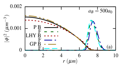
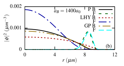
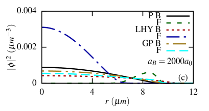
Figure 3: (Color online) Densities of Bose ($|\phi_{B}|^{2}$) and Fermi ($|\phi_{F}|^{2}$) components in a harmonically trapped ⁷Li-⁶Li mixture from a solution of Eqs. (25)-(26) by imaginary-time propagation: present (P) crossover model, Eqs. (8) and (19); LHY (LHY) model, Eq. (28); and GP-DF (GP) model, Eq. (29); for $a_{\rm B}=$ (a) $500a_{0}$, (b) $1400a_{0}$, and (c) $2000a_{0}$. The other parameters, $N_{B}=50000$, $N_{F}=1000a_{0}$, $a_{\rm F}=0$, and $a_{\rm BF}=1500a_{0}$, are the same for (a)-(c).

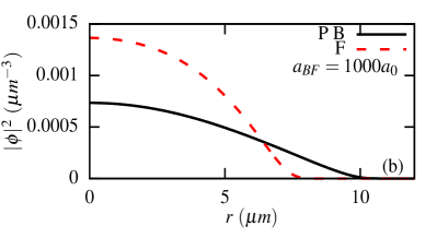
Figure 4: (Color online) Same as in Fig. 3 for parameters (a) $a_{B}=\infty,a_{BF}=1500a_{0}$ and (b) $a_{B}=\infty,a_{BF}=1000a_{0}$ for the present (P) crossover model, other parameters are the same as in Fig. 3.

The solutions obtained with the present crossover model which smoothly connects the weak-coupling regime with the unitarity regime are compared with the two models applicable in the weak-coupling regime, i.e. the GP-DF and LHY models. Before we proceed, let us precisely state what we mean by these three models. Solutions of Eqs. (25) and (26) with $f(x=a_{B}N_{B}^{1/3}|\phi_{B}|^{2/3})$ and $g(y=a_{F}k_{F})$ given, respectively, by Eqs. (8) and (19) are termed as solutions obtained by the present model (denoted by symbol $P$ for present). In the LHY and GP-DF models, $f(x)$ and $g(y)$ in Eqs. (25) and (26) are given, respectively, by

$$f(x) =4\pi\left(x+\frac{\alpha}{2}x^{5/2}\right),\quad g(y)=1+d_{1}y+d_{2}y^{2};$$ (28)

$$f(x) =4\pi x,\quad g(y)=1.$$ (29)

We find that the ground state solution of the present model can be different quantitatively as well as qualitatively from the LHY and GP-DF models.

We find that without the inter-species interaction ($a_{BF}=0$) the density of both components is maximum at the center resulting in a mixed phase. With the increase of repulsive inter-species interaction the density of one of the components may reduce at the center. With further increase of inter-species repulsion the density of one of the components could be zero at the center and when that happens we will call the resultant Bose-Fermi state a demixed state.

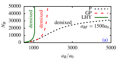
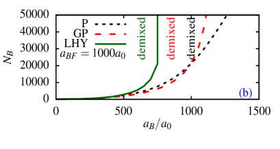
Figure 5: $N_{\rm B}$-$a_{\rm B}$ phase plots illustrating the mixing and demixing domains from the present (P) crossover, GP-DF (GP), LHY (LHY) models for (a) $N_{\rm F}=1000,a_{\rm F}=0,$ and $a_{\rm BF}=1500a_{0}$ and (b) $N_{\rm F}=1000,a_{\rm F}=0,$ and $a_{\rm BF}=1000a_{0}$. The demixed (mixed) states with the three models lie towards the left (right) of the respective lines.

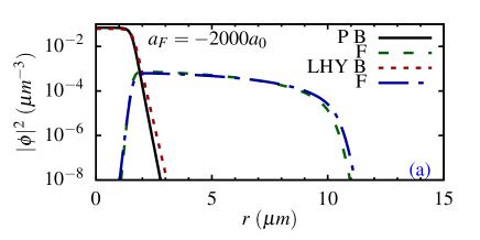
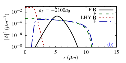
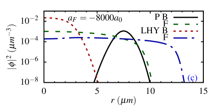
Figure 6: (Color online) Densities of Bose ($|\phi_{B}|^{2}$) and Fermi ($|\phi_{F}|^{2}$) components in a harmonically trapped ⁷Li-⁶Li mixture from the present (P) crossover model, Eqs. (25)-(26), and the LHY (LHY) model, Eq. (28) for $a_{\rm F}=$ (a) $-2000a_{0}$, (b) $-2100a_{0}$, and (c) $-8000a_{0}$. The other parameters, $N_{B}=1000$, $N_{F}=50000a_{0}$, $a_{\rm B}=500a_{0}$, and $a_{\rm BF}=1500a_{0}$, are the same for (a)-(c).

We first consider a Bose-Fermi ⁷Li-⁶Li mixture with $N_{\rm B}=50000,N_{\rm F}=1000$, $a_{\rm F}=0,a_{\rm BF}=1500a_{0}$ for different $a_{\rm B}$. In Figs. 3 we plot component densities $|\phi_{i}(r)|^{2}$ for the three models normalized as $4\pi\int r^{2}dr|\phi_{i}(r)|^{2}=1$. For $a_{\rm B}=500a_{0}$, there is a good agreement between the component densities obtained from the three models as is shown in Fig. 3(a), which indicates that the system is in the weak-coupling regime. As $a_{\rm B}$ is increased progressively to (b) $1400a_{0}$ and (c) $2000a_{0}$, in both the LHY and GP-DF models, the system slowly changes from demixed state to mixed state with the transition first occurring for the LHY model, viz. Figs. 3 (a)-(b), and then for the GP-DF model, viz. Figs. 3(b)-(c); whereas in the present model the system remains always demixed. On further increase in $a_{\rm B}$, the system remains demixed as per the present model as shown in Fig. 4(a) for $a_{\rm B}=\infty$. However, a large $a_{BF}$ ($=1500a_{0}$) is necessary for demixing in the present model and for a slightly smaller $a_{BF}$ ($=1000a_{0}$), we have mixing in the present model, viz. Fig. 4(b). Hence the qualitative difference among the results of the present model on one hand and the LHY and the GP-DF models on the other hand as found in Figs. 3, as $a_{B}$ is changed from weak to strong coupling, is caused by a relatively large value of $a_{BF}$ ($=1500a_{0}$) used in numerical simulation. If we used the value $a_{BF}=1000a_{0}$ instead, keeping all other parameters unchanged, we verified that there will not be any qualitative difference in the results of the three models: as $a_{B}$ is increased from weak to strong coupling in all three models there will be transition from demixed to mixed configuration (figure not presented). The same will be true for the physical value $a_{BF}=40a_{0}$ for the Bose-Fermi scattering length in the ⁷Li-⁶Li system expbf .

Here we are using a large value of $a_{BF}$ in the range $1000a_{0}\sim 1500a_{0}$, and are using a mean-field GP-type Bose-Fermi repulsion valid for small values of the gas parameter $x_{BF}\equiv a_{BF}(n_{BF})^{1/3}\lessapprox 0.2$, where $n_{BF}$ is the geometric mean of Bose and Fermi densities. From Figs. 3 and 4, we find that the typical average values of $|\phi_{i}|^{2}$ are less than 0.0005 and the densities are $n_{i}=N_{i}|\phi_{i}|^{2}$ with $N_{B}=50000$, $N_{F}=1000$ and $a_{BF}=1500a_{0}$; consequently, $x_{BF}\approx 0.12<0.2$, where the GP approximation for Bose-Fermi interaction is valid. In these figures the bosonic gas parameter with $N_{B}=50000$ and $a_{B}=1500a_{0}$ is larger than 0.2, thus requiring the present crossover formula for a proper description of dynamics.

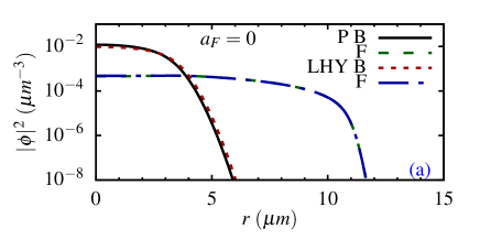
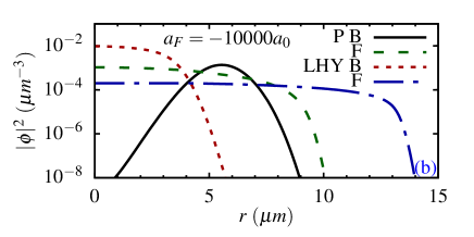
Figure 7: (Color online) Same as in Fig. 6 for $N_{B}=1000,N_{F}=50000,a_{BF}=1000a_{0},a_{B}=1000a_{0},$ and (a) $a_{F}=0$, and (b) $a_{F}=-10000a_{0}$.

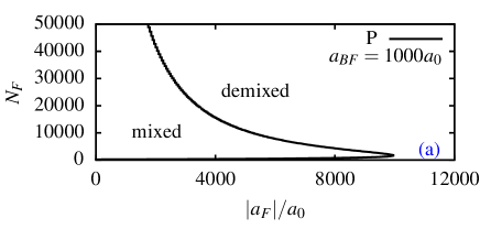
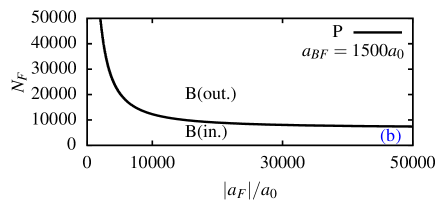
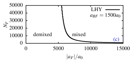
Figure 8: $N_{\rm F}$-$|a_{\rm F}|$ phase plots for $N_{B}=1000,a_{B}=500a_{0}$ and illustrating (a) the mixing and demixing domains for the present (P) model with $a_{BF}=1000a_{0}$, (b) crossover between the demixed state with bosons (fermions) forming the core (shell) to the demixed state with bosons (fermions) forming the shell (core) for present model with $a_{BF}=1500a_{0}$, and (c) the demixing and mixing domains for the LHY (LHY) model with $a_{BF}=1500a_{0}$.

Keeping $N_{\rm F}$ and $a_{\rm F}$ fixed, the $N_{\rm B}$-$a_{\rm B}$ phase plots showing the parameter domains of mixed and demixed states are illustrated in Figs. 5(a) and (b) for $a_{BF}=1500a_{0}$ and $1000a_{0}$, respectively. The demixed (mixed) states for the present, GP-DF, and LHY models appear on the left (right) side of the respective lines.

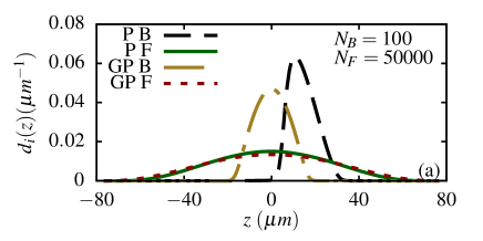
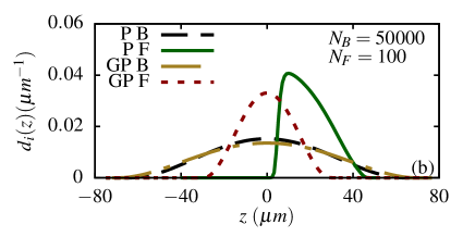
Figure 9: Reduced density $d_{i}(z)$ of the binary Bose-Fermi mixture for (a) $N_{B}=100$, $N_{F}=50000$, $a_{\rm B}=4000a_{0},a_{\rm F}=-4000a_{0},a_{\rm BF}=1500a_{0}$, (b) $N_{B}=50000$, $N_{F}=100$, $a_{\rm B}=4000a_{0},a_{\rm F}=-4000a_{0},a_{\rm BF}=1500a_{0}$ for the present (P) and GP-DF (GP) models. Here $\omega_{z}=0.1\omega_{x}$

Let us consider another case with $N_{\rm B}=1000,N_{\rm F}=50000$, $a_{\rm B}=500a_{0},a_{\rm BF}=1500a_{0}$, while $a_{\rm F}$ is progressively decreased. In this case, for $-2000a_{0}\leq a_{F}<0$, the three models lead to qualitatively similar demixing with the Bose component forming a core with the Fermi component forming a shell surrounding it as shown in Fig. 6(a) for $a_{F}=-2000a_{0}$. The results of the GP-DF model are independent of $a_{\rm F}$, and hence in Fig. 6 we do not show the results of this model. As $a_{\rm F}$ is decreased slightly to $a_{F}=-2100a_{0}$, we find a Bose component forming a shell outside a Fermi core at the center as per the present model as is shown in Fig. 6(b) for $a_{F}=-2100a_{0}$. Upon further reduction of $a_{\rm F}$ to $-8000a_{0}$, the Bose shell moves further away from the center of the trap according to the present model, whereas LHY model ends up in the mixed phase as is shown in Fig. 6(c).

If we perform the analysis illustrated in Fig. 6 for $a_{BF}=1000a_{0}$, the inter-species repulsion is weaker and in the weak-coupling limit ($a_{F}=0$), we have overlapping states for all models as shown in Fig. 7(a). Again we do not show the results of the GP-DF model as the same do not change with $a_{F}$. In the strong-coupling limit ($a_{F}=-10000a_{0}$), the present model results in the demixed state, whereas the LHY model remains in the mixed state, viz. Fig. 7(b).

The mixing-demixing phenomena illustrated in Figs. 6 and 7 leads to the $N_{F}$-$|a_{F}|$ phase plots of Figs. 8. In Fig. 8(a) the fixed parameters are $N_{B}=1000,a_{B}=500a_{0}$ and $a_{BF}=1000a_{0}$. In this case mixing-demixing transition takes place only for the present model for $N_{F}\geq 270.$ In Fig. 8(b), with fixed parameters $N_{B}=1000,a_{B}=500a_{0},a_{BF}=1500a_{0}$, the present model, which results in a demixed ground state, predicts a position-swapping transition with the Bose component forming the core which is surrounded by the fermionic shell below a critical $N_{F}$ for a given value of $a_{F}$ (as is shown in Fig. 6(a)). Above this critical $N_{F}$, the Fermi component moves to the core with the Bose component forming the shell around it as in Fig. 6(c). These two qualitatively different states are marked as B(in) and B(out), respectively, in Fig. 8(b). For the same fixed parameters $N_{B}=1000,a_{B}=500a_{0},a_{BF}=1500a_{0}$, the LHY model leads to the demixing-mixing transition as one increases $N_{F}$ at the fixed value of $a_{F}$ as is shown in Fig. 8(c).

Next we consider a quasi-1D ⁷Li-⁶Li Bose-Fermi mixture Q1D along the $z$ axis with strong traps in the $x-y$ plane ($\omega_{x}=10\omega_{z}$) and consider a few illustrative examples to show the qualitatively different ground state solutions obtained from the present model as compared to the GP-DF and LHY models. The spatial step size $\Delta x=\Delta y=\Delta z$ and time step $\Delta t$ used to solve Eqs. (25)-(26) numerically are $0.15$ and $0.005625$, respectively, in dimensionless units. In such a quasi-1D Bose-Fermi mixture, the essential collective dynamics and mixing-demixing transition take place in the $z$ direction. Hence for quasi-1D ⁷Li-⁶Li Bose-Fermi mixtures, we will illustrate only the reduced 1D density along the $z$ direction $d_{i}(z)=\int dxdy|\phi_{i}(x,y,z)|^{2}$. Apart from mixing-demixing transition in the $z$ direction, we also find spontaneous symmetry-broken states in the quasi-1D ⁷Li-⁶Li Bose-Fermi mixtures. Two examples of spontaneous symmetry breaking in the present model are shown in Fig. 9(a)-(b) for the reduced 1D density along $z$ direction where one of the components moved away from the center breaking the parity symmetry. In this case the results of the GP-DF and LHY models lie very close to each other and the result of only the former model is shown. In Figs. 9 there is a demixing in the present crossover model with the density of one of the components being zero at the center while the other component having a density maximum at the center. The densities of the LHY model remain overlapping and parity symmetric.

In addition to the spontaneous symmetry broken states of Fig. 9, it is also possible to have partially to fully demixed states in quasi-1D Bose-Fermi mixtures. For this purpose, we consider (a) $\omega_{x}=10\omega_{z}$ and (b) $\omega_{x}=100\omega_{z}$ , where the spatial step size $\Delta x=\Delta y=\Delta z$ and time step $\Delta t$ used to solve the equations (25)-(26) numerically are taken to be $0.1$ and $0.0025$, respectively. For both (a) and (b), we consider $N_{\rm B}=1000$, $N_{\rm F}=100,a_{B}=500a_{0},a_{\rm F}=-20000a_{0}$, and $a_{\rm BF}=1500a_{0}$. The reduced 1D density $d_{i}(z)$ obtained in these two cases with the present and GP-DF models are shown in Figs. 10(a) and (b); it is evident that the bosons stay in the central region and the fermions are expelled symmetrically in two directions. With the present model, the ground state is partially demixed with $\omega_{x}=10\omega_{z}$, viz. Fig. 10(a) and fully demixed with $\omega_{x}=100\omega_{z}$, viz. Fig. 10(b). In the GP-DF models, there is partial demixing which becomes more pronounced as the trap becomes more confined along the radial direction; the same is the case with LHY model (not shown in the figure).

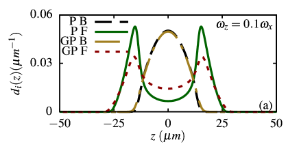
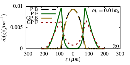
Figure 10: Reduced density $d_{i}(z)$ of the binary mixture for $N_{B}=1000$, $N_{F}=100$, $a_{\rm B}=500a_{0},a_{\rm F}=-20000a_{0},a_{\rm BF}=1500a_{0}$ with (a) $\omega_{z}=0.1\omega_{x}$ and (b) $\omega_{z}=0.01\omega_{x}$ for the present (P) and GP-DF (GP) models.

IV SUMMARY

Here we have demonstrated spontaneous symmetry breaking and mixing-demixing transition in trapped super-fluid Bose-Fermi mixture along the crossover from weak-coupling to unitarity for both intra-species Bose and Fermi interactions. For Bose-Fermi inter-species interaction, we have used the weak-coupling GP interaction. The usual description of the super-fluid Bose-Fermi mixture employs the weak-coupling GP Lagrangian for the bosons and DF Lagrangian for the fermions. The interaction term in the GP Lagrangian is essentially the same as the many-body Hartree interaction term; that in the DF Lagrangian is the total kinetic energy of the fermions in the Fermi sea. Usual treatment of the Bose-Fermi mixture employing GP Lagrangian for bosons and DF Lagrangian for fermions is termed GP-DF formulation. To study the Bose-Fermi mixture along the weak-to-strong coupling crossover, we suggested analytic non-perturbative Lagrangians for intra-species Bose and Fermi interactions with correct LHY limit(s) in the weak-coupling domain and with correct unitarity limit(s) in the strong-coupling domain. These analytic Lagrangians have a single parameter: the universal parameter(s) $\eta_{i}$ at unitarity for bosons and fermions. In this study we have used the most precise value(s) of this universal parameter, which should be updated in future applications, if possible. The Euler-Lagrange equations of the Bose-Fermi mixture describe the dynamics and have been used in this study.

In this study, we considered spherically-symmetric and quasi-1D traps. In both cases, we compared the results of the present model valid along the crossover with those of the usual weak-coupling GP-DF and LHY models and found that the two types of treatments may lead to qualitatively different results. For example, in spherically symmetric traps we identified cases of demixing in Bose-Fermi mixture using the present crossover model not found in the weak-coupling GP-DF and LHY models. In quasi-1D traps, we found spontaneous symmetry breaking in the present crossover model not found in GP-DF and LHY models. Hence we conclude that the perturbative LHY model is unable to properly describe the Bose-Fermi mixture away from the weak-coupling limit.

- (1) M. H. Anderson, J. R. Ensher, M. R. Matthews, C. E. Wieman, and E. A. Cornell, Science 269, 198 (1995); K. B. Davis, M.-O. Mewes, M. R. Andrews, N. J. van Druten, D. S. Durfee, D. M. Kurn, and W. Ketterle, Phys. Rev. Lett. 75, 3969 (1995).
- (2) B. de Marco and D. Jin, Science 285, 1703 (1999).
- (3) F. Schreck, L. Khaykovich, K. L. Corwin, G. Ferrari, T. Bourdel, J. Cubizolles, and C. Salomon, Phys. Rev. Lett. 87, 080403 (2001); A. G. Truscott, K. E. Strecker, W. I. McAlexander, G. B. Partridge, R. G. Hulet, Science 291, 5513 (2001); G. Roati, F. Riboli, G. Modugno, and M. Inguscio, Phys. Rev. Lett. 89, 150403 (2002); Z. Hadzibabic, S. Gupta, C. A. Stan, C. H. Schunck, M. W. Zwierlein, K. Dieckmann, and W. Ketterle, Phys. Rev. Lett. 91, 160401 (2003).
- (4) F. Dalfovo, S. Giorgini, L. P. Pitaevskii, and S. Stringari, Rev. Mod. Phys. 71, 463 (1999).
- (5) S. Giorgini, L. P. Pitaevskii, and S. Stringari, Rev. Mod. Phys. 80, 1215 (2008).
- (6) K. Mølmer Phys. Rev. Lett. 80, 1804 (1998); N. Nygaard and K. Mølmer Phys. Rev. A 59, 2974 (1999); Z. Akdeniz, P. Vignolo, M.P. Tosi, J. Phys. B 38, 2933 (2005); K. Suzuki, T. Miyakawa, and T. Suzuki, Phys. Rev. A 77, 043629 (2008); C. Ufrecht, M. Meister, A. Roura, and W. P. Schleich, New J. Phys. 19, 085001 (2017); H. P. Büchler and G. Blatter, Phys. Rev. A 69, 063603 (2004); K. K. Das, Phys. Rev. Lett. 90, 170403 (2003); M. A. Cazalilla and A. F. Ho Phys. Rev. Lett. 91, 150403 (2003); A. Imambekov and E. Demler Phys. Rev. A 73, 021602(R) (2006); S. G. Bhongale and H. Pu, Phys. Rev. A 78, 061606(R) (2008).
- (7) S. K. Adhikari and L. Salasnich, Phys. Rev. A 78, 043616 (2008).
- (8) C. Chin, R. Grimm, P. Julienne, and E. Tiesinga, Rev. Mod. Phys. 82, 1225 (2010); S. Inouye, M. R. Andrews, J. Stenger, H.-J. Miesner, D. M. Stamper-Kurn, and W. Ketterle, Nature (London) 392, 151 (1998).
- (9) I. Ferrier-Barbut, M. Delehaye, S. Laurent, A. T. Grier, M. Pierce, B. S. Rem, F. Chevy, and C. Salomon, Science 345, 1035 (2014); R. Roy, A. Green, R. Bowler, and S. Gupta, Phys. Rev. Lett. 118, 055301 (2017); M. Delehaye, S. Laurent, I. Ferrier-Barbut, S. Jin, F. Chevy, and C. Salomon, Phys. Rev. Lett. 115, 265303 (2015); T. Ozawa, A. Recati, M. Delehaye, Fredéric Chevy, and S. Stringari, Phys. Rev. A 90, 043608 (2014); X. Cui, Phys. Rev. A 90, 041603(R) (2014); J. J. Kinnunen and G. M. Bruun, Phys. Rev. A 91, 041605(R) (2015).
- (10) U. Eismann, L. Khaykovich, S. Laurent, I. Ferrier-Barbut, B. S. Rem, A. T. Grier, M. Delehaye, F. Chevy, C. Salomon, L.-C. Ha, and C. Chin, Phys. Rev. X 6, 021025 (2016); W. Li and T.-L. Ho, Phys. Rev. Lett. 108, 195301 (2012); P. Makotyn, C. E. Klauss, D. L. Goldberger, E. A. Cornell, and D. S. Jin, Nature Phys. 10, 116 (2014); C. Eigen, J. A. P. Glidden, R. Lopes, N. Navon, Z. Hadzibabic, and R. P. Smith, Phys. Rev. Lett. 119, 250404 (2017).
- (11) Y.Castin and F.Werner, Lecture Notes in Physics, 836, 127 (2012).
- (12) N. Navon, S. Nascimbène, F. Chevy, and C. Salomon, Science 328, 729 (2010).
- (13) S. Nascimbène, N. Navon, K. J. Jiang, F. Chevy, and C. Salomon, Nature (London) 463, 1057 (2010).
- (14) G. B. Partridge, W. Li, R. I. Kamar, Y. Liao, R. G. Hulet, Science 311, 503 (2006).
- (15) J. T. Stewart, J. P. Gaebler, C. A. Regal, and D. S. Jin, Phys. Rev. Lett. 97, 220406 (2006).
- (16) M. Randeria and E. Taylor, Ann. Rev. Cond. Matter Phys. 5, 209 (2014).
- (17) A. Sen, J. High Energy Phys. 12, 115 (2016).
- (18) P. van Wyk, H. Tajima, D. Inotani, A. Ohnishi, and Y. Ohashi, Phys. Rev. A 97, 013601 (2018).
- (19) D. G. Levkov, A. G. Panin, and I. I. Tkachev, Phys. Rev. Lett. 118, 011301 (2017); R. Ruffini and S. Bonazzola, Phys. Rev. 187, 1767 (1969); I. I. Tkachev, Sov. Astron. Lett. 12, 305 (1986); P. H. Chavanis, Phys. Rev. D 84, 043531 (2011); P. H. Chavanis and L. Delfini, Phys. Rev. D 84, 043532 (2011).
- (20) H. Heiselberg, Lecture Notes in Physics 836, 49 (2012).
- (21) E.P. Gross, Nuovo Cim. 20, 454 (1961); L.P. Pitaevskii, Sov. Phys. JETP. 13, 451 (1961).
- (22) T. D. Lee, K. Huang, and C. N. Yang, Phys. Rev. 106, 1135 (1957).
- (23) K. Huang and C. N. Yang, Phys. Rev. 105, 767 (1957); T. D. Lee and C. N. Yang, Phys. Rev. 105, 1119 (1957).
- (24) S. K. Adhikari and L. Salasnich, Phys. Rev. A 77, 033618 (2008).
- (25) N. Manini and L. Salasnich, Phys. Rev. A 71, 033625 (2005); Y. E. Kim and A. L. Zubarev, Phys. Rev. A 70, 033612 (2004); G. Diana, N. Manini, and L. Salasnich, Phys. Rev. A 73, 065601 (2006); L. Salasnich and N. Manini, Laser Phys. 17, 169 (2007); L. Salasnich, N. Manini, and A. Parola, Phys. Rev. A 72, 023621 (2005); S. K. Adhikari, Phys. Rev. A 77, 045602 (2008).
- (26) L. Tonks, Phys. Rev. 50, 955 (1936); M. Girardeau, J. Math. Phys. 1, 516 (1960).
- (27) D, S. Sholl and J. A. Steckel, Density Functional Theory: A Practical Introduction, (John Wiley & Sons, 2009).
- (28) L. N. Cooper, Phys. Rev. 104, 1189 (1956).
- (29) S. K. Adhikari, J. Phys. B 43, 085304 (2010); F. Kh. Abdullaev, M. Ögren, and M. P. Sorensen, Phys. Rev. A 99, 033614 (2019); W. Wen and H.-J. Li, New J. Phys. 20, 083044 (2018); A. Mitra, J. Low Temp. Phys. 190, 90 (2018); W. Wen, B. Y. Chen, and X. W. Zhang, J. Phys. B 50, 035301 (2017); M. Tylutki, A. Recati, F. Dalfovo, and S. Stringari, New J. Phys. 18, 053014 (2014); D. Lacroix, Phys. Rev. A94, 043614 (2016).
- (30) L. Wen and J. Li, Phys. Rev. A 90, 053621 (2014); W. Wen, C. Zhao, and X. Ma, Phys. Rev. A 88, 063621 (2013); T.-L. Song, C. R. Ma, and Y.-L. Ma, Ann. Phys. 327, 1933 (2012).
- (31) D. Lacroix, A. Boulet, M. Grasso, and C. J.Yang, Phys. Rev. C 95, 054306 (2017), A. Boulet and D. Lacroix, Phys. Rev. C 97, 041301 (2018); L. Zhang, W. Wen, X.-D. Ma, and Y. Wang, Int. J. Mod. Phys. B 32, 1850230 (2018); M. Yan, W.-S. Duan, F.-Q. Dou, X.-Q. Gou, and H. Zhang, Eur. Phys. J. B 87, 180 (2014); W. Wen and Hui-jun Li, J. Phys. B: At. Mol. Opt. Phys. 46, 035302 (2013).
- (32) L. D. Landau, J. Phys. USSR. 5, 71, (1941).
- (33) G. E. Astrakharchik, R. Combescot, X. Leyronas, and S. Stringari, Phys. Rev. Lett. 95, 030404 (2005).
- (34) S. K. Adhikari and L. Salasnich, Sci. Rep. 8, 8825 (2018).
- (35) J. L. Song and F. Zhou, Phys. Rev. Lett. 103, 025302 (2009); Yu-Li Lee and Yu-Wen Lee, Phys. Rev. A 81, 063613 (2010); J. M. Diederix, T. C. F. van Heijst, and H. T. C. Stoof, Phys. Rev. A 84, 033618 (2011); F. Zhou and M. S. Mashayekhi, Ann. Phys. 328, 83 (2013); M. Rossi, L. Salasnich, F. Ancilotto, and F. Toigo, Phys. Rev. A 89, 041602 (2014).
- (36) Y. Ding and C. H. Greene, Phys. Rev. A 95, 053602 (2017).
- (37) J. Bardeen, L. N. Cooper, and J. R. Schrieffer, Phys. Rev. 106, 162 (1957).
- (38) C. F. von Weizsäcker, Z. für Physik 96, 431 (1935).
- (39) G. E. Astrakharchik, J. Boronat, J. Casulleras, and S. Giorgini, Phys. Rev. Lett. 95, 230405 (2005).
- (40) P. Pieri and G. C. Strinati, Phys. Rev. Lett. 91, 030401 (2003).
- (41) S. Chang, V. Pandharipande, J. Carlson, and K. Schmidt, Phys. Rev. A 70, 043602 (2004).
- (42) G. E. Astrakharchik, J. Boronat, J. Casulleras, and S. Giorgini, Phys. Rev. Lett. 93, 200404 (2004).
- (43) S. Pilati and S. Giorgini, Phys. Rev. Lett. 100, 030401 (2008).
- (44) M. Horikoshi, M. Koashi, H. Tajima, Y. Ohashi, and M. Kuwata-Gonokami, Phys. Rev. X 7, 041004 (2017).
- (45) M. J. H. Ku, A. T. Sommer, L. W. Cheuk, and M. W.Zwierlein, Science 335, 563 (2012).
- (46) S. Gandolfi, K. E. Schmidt, and J. Carlson, Phys. Rev. A 83, 041601 (2011).
- (47) R. Haussmann, W. Rantner, S. Cerrito, and W. Zwerger, Phys. Rev. A 75, 023610 (2007).
- (48) H. Hu, X.-J. Liu, and P. D. Drummond, Europhys. Lett. 74, 574 (2006).
- (49) A. Bulgac, J. E. Drut, and P. Magierski, Phys. Rev. A 78, 023625 (2008).
- (50) H. Tajima, R. Hanai, and Y. Ohashi, Phys. Rev.A 93, 013610 (2016); H. Tajima, P. van Wyk, R. Hanai, D. Kagamihara, D.Inotani, M. Horikoshi, and Y. Ohashi, Phys. Rev. A 95, 043625 (2017).
- (51) P. Muruganandam and S. K. Adhikari, Comput. Phys. Commun. 180, 1888 (2009); D. Vudragović, I. Vidanović, A. Balaž, P. Muruganandam, and S. K. Adhikari, Comput. Phys. Commun. 183, 2021 (2012).
- (52) L. E. Young-S., D. Vudragović, P. Muruganandam, S. K. Adhikari, A. Balaž, Comput. Phys. Commun. 204, 209 (2016); L. E. Young-S., P. Muruganandam, S. K. Adhikari, V. Loncar, D. Vudragovic, A. Balaž, Comput. Phys. Commun. 220, 503 (2017).
- (53) P. Muruganandam and S. K. Adhikari, J. Phys. B 36, 2501 (2003).
- (54) S. Laurent, M. Pierce, M. Delehaye, T. Yefsah, F. Chevy, and C. Salomon, Phys. Rev. Lett. 118, 103403 (2017).
- (55) S. K. Adhikari and L. Salasnich, New J. Phys. 11, 023011 (2009).