Phase Diagram of Bipartite Entanglement

Abstract

We investigate the features of the entanglement spectrum (distribution of the eigenvalues of the reduced density matrix) of a large quantum system in a pure state. We consider all Rényi entropies and recover purity and von Neumann entropy as particular cases. We construct the phase diagram of the theory and unveil the presence of two critical lines.

1 Introduction

The notion of entanglement is central in the emerging fields of quantum technologies and quantum applications [1]. Entanglement is a genuine non-classical feature of quantum states [2] and characterizes the nonclassical correlations among the different components of a quantum system. It can be measured in terms of different quantities, such as purity and von Neumann entropy [3, 4, 5].

For large quantum systems, the distribution of bipartite entanglement is pivotal to understand the features of the many-body wave function. Interestingly, random pure states play a crucial role in this context: they are characterized by a large entanglement and display a number of interesting features. The first studies on this subject date back to forty years ago and focused on the average purity of a bipartite system, that turns out to be almost minimal for randomly sampled states [6]. These findings were extended to the average von Neumann entropy [7, 8, 9, 10] and to higher moments [11], and are essentially a consequence of the concentration of measure for the so-called entanglement spectrum (the eigenvalues of the reduced density matrix) [12].

The typical entanglement spectrum was eventually determined [13, 14, 15] and displayed the presence of phase transitions. These studies focused on the purity, and were soon extended to different Rényi entropies [16, 17] and eventually to the von Neumann entropy [18]. It is in fact somewhat surprising that a number of interesting results can be obtained analytically, probably because they hinge on the Coulomb gas method [19, 20] and the ensuing saddle point equations [21, 22, 23, 24].

In the approach proposed in Ref. [13] one “biases” the amount of entanglement across the (given) bipartition and studies typicality constrained at such entanglement. This yields a family of entanglement spectra that depend on the adopted measure of entanglement and whose features are of great interest. One unveils the presence of two phase transitions, as the entanglement between the two partitions is changed. One of them is related to the “evaporation” of the largest eigenvalue, which splits off from the continuous distribution of eigenvalues [25, 26], while the other one to the vanishing of the smallest eigenvalue and to the squeezing of the distribution against the hard wall at zero (pushed-to-pulled transition) [27, 28, 29, 30, 31].

In this Article we shall scrutinize the features of these phase transitions for all Rényi entropies. We shall find that, as anticipated in [18], the phase transitions for the von Neumann entropy are smoother than for all Rényi entropies, and in particular one of them becomes continuous when the other one is of first order.

This work is organized as follows. We define the problem and set up our notation in Section 2. The entangled, typical and separable phases are analyzed in Secs. 3, 4 and 5, respectively. The phase diagram is drawn in Sec. 6. We conclude in Sec. 7.

2 Setting up the problem

Consider a bipartite system in the Hilbert space $\mathcal{H}=\mathcal{H}_{A}\otimes\mathcal{H}_{\bar{A}}$, described by a pure state $|\psi\rangle$. The reduced density matrix of subsystem $A$,

$$\varrho_{A}=\tr_{\bar{A}}|\psi\rangle\langle\psi|,$$ (1)

is a (Hermitian) positive matrix of unit trace, $\tr\varrho_{A}=1$. We quantify the bipartite entanglement between $A$ and $\bar{A}$ by the Rényi entropy of $\varrho_{A}$,

$$S_{q}(\vec{\lambda})=-\frac{1}{q-1}\ln\!\left(\sum_{k=1}^{N}\lambda_{k}^{q}\right),$$ (2)

where $N=\dim\mathcal{H}_{A}$, $\vec{\lambda}=(\lambda_{1},\dots,\lambda_{N})\in\Delta_{N-1}$ are the eigenvalues (Schmidt coefficients) of $\varrho_{A}$, and $\Delta_{N-1}$ is the simplex of eigenvalues ($\lambda_{k}\geq 0$, $\sum_{k}\lambda_{k}=1$). We are interested in balanced bipartitions: $N=\dim\mathcal{H}_{A}=\dim\mathcal{H}_{\bar{A}}$. The Rényi entropy ranges $0\leq S_{q}\leq\ln N$, where the minimum and maximum values are obtained, respectively, for separable and maximally entangled vector states $|\psi\rangle$. Note that the Rényi entropy reduces to the von Neumann entropy $S_{1}=-\sum_{k}\lambda_{k}\ln\lambda_{k}$ in the limit $q\to 1$.

We will focus on the typical features of the afore-mentioned eigenvalues. For random states $|\psi\rangle$, uniformly sampled on the unit sphere $\langle\psi|\psi\rangle=1$, the eigenvalues $\vec{\lambda}$ are distributed according to the (Haar) joint probability density function [32, 33, 34]

$$p_{N}(\vec{\lambda})=C_{N}\prod_{1\leq j<k\leq N}{(\lambda_{j}-\lambda_{k})^{2}},$$ (3)

$C_{N}$ being a normalization factor. For large $N$, the distribution $p_{N}$ concentrates around a typical set $\vec{\lambda}$, that maximizes $p_{N}$ [12], and the typical spectral distribution of $\varrho_{A}$ follows a Marčenko-Pastur law [35] with support $[0,4/N]$ [18].

We shall ask here how the entanglement spectrum is distributed in a system with a given amount of bipartite entanglement, conditioned at a given value of the entropy $S_{q}$. This is nothing but a constrained maximization problem. Let

$$u=\ln N-S_{q}(\vec{\lambda})=\frac{1}{q-1}\ln\!\left(\frac{1}{N}\sum_{k}(N\lambda_{k})^{q}\right),$$ (4)

which quantifies the deviation of the entropy $S_{q}$ from its maximum value $\ln N$. Then, given a value $u\in[0,\ln N]$, we seek $\vec{\lambda}_{\mathrm{max}}$ such that

$$p_{N}(\vec{\lambda}_{\mathrm{max}})=\max\left\{p_{N}(\vec{\lambda})\,:\,\vec{\lambda}\in\Delta_{N-1},\,S_{q}(\vec{\lambda})=\ln N-u\right\}.$$ (5)

Introducing two Lagrange multipliers $\xi$ and $\beta$, that constrain the eigenvalue normalization and the deviation $u$ of the entropy from its maximum $\ln N$, respectively, the problem is translated into the (unconstrained) minimization of the potential

$$V(\vec{\lambda},\xi,\beta) = {-\frac{2}{N^{2}}}\sum_{j<k}\ln|\lambda_{j}-\lambda_{k}|+\xi\left(\sum_{k}\lambda_{k}-1\right)$$ (6)

$$+\beta\left[\frac{1}{q-1}\ln\!\left(\frac{1}{N}\sum_{k}(N\lambda_{k})^{q}-\sum_{k}\lambda_{k}+1\right)-u\right]$$

with respect to $\vec{\lambda}$, $\xi$, and $\beta$. Note that we have added two terms in the logarithm that expresses the constraint on the entropy; otherwise, the expression is not well defined for $q\to 1$ before imposing the other constraint on the eigenvalue normalization. The potential $V$ can be viewed as the energy of a gas of point charges (eigenvalues) distributed in the interval $[0,1]$ with a 2D (logarithmic) Coulomb repulsion, subject to two external electric fields proportional to $\xi$ and $\beta$. The logarithmic form of the interaction is a direct consequence of the product form (3) of the joint probability density.

It is worth noting that this problem can be equivalently framed in the statistical mechanics of points on the simplex $\Delta_{N-1}$ with partition function [18]

$$Z_{N}=\int_{\Delta_{N-1}}\rme^{-\beta N^{2}E(\vec{\lambda})}p_{N}(\vec{\lambda})\,\rmd^{N}\lambda,$$ (7)

with an “energy density” $E(\vec{\lambda})=\ln N-S_{q}(\vec{\lambda})$ and an inverse “temperature” $\beta$. In the thermodynamic limit $N\to\infty$, one looks at the maximum of the integrand, that is at the minimum of the potential (6). Large values of $\beta$ yield highly entangled states, while $\beta=0$ yields random states.

The saddle-point equations read

$$\qquad\quad\frac{\partial V}{\partial\lambda_{j}}=\frac{2}{N}\sum_{k\neq j}\frac{1}{N\lambda_{k}-N\lambda_{j}}+\frac{\beta}{q-1}\frac{q(N\lambda_{j})^{q-1}-1}{\displaystyle\frac{1}{N}\sum_{k}(N\lambda_{k})^{q}-\frac{1}{N}\sum_{k}N\lambda_{k}+1}+\xi=0,$$ (8)

$$\qquad\quad\frac{\partial V}{\partial\beta}=\frac{1}{q-1}\ln\!\left(\frac{1}{N}\sum_{k}(N\lambda_{k})^{q}-\frac{1}{N}\sum_{k}N\lambda_{k}+1\right)-u=0,$$ (9)

$$\qquad\quad\displaystyle\frac{\partial V}{\partial\xi}=\frac{1}{N}\sum_{k}N\lambda_{k}-1=0.$$ (10)

When all the eigenvalues $\lambda_{k}$ are of order $O(1/N)$, we introduce the empirical eigenvalue distribution

$$\sigma(\lambda)=\frac{1}{N}\sum_{k}\delta(\lambda-N\lambda_{k}),$$ (11)

with

$$\int\rmd\lambda\,\sigma(\lambda)=1,$$ (12)

and Eqs. (8)–(10) read

$$2\fint\rmd\lambda^{\prime}\,\frac{\sigma(\lambda^{\prime})}{\lambda^{\prime}-\lambda}+\beta\rme^{-(q-1)u}\frac{q\lambda^{q-1}-1}{q-1}+\xi=0,$$ (13)

$$\int\rmd\lambda\,\sigma(\lambda)\lambda=1,$$ (14)

$$u=\frac{1}{q-1}\ln\!\left(\int\rmd\lambda\,\sigma(\lambda)\lambda^{q}\right),$$ (15)

with $\lambda=N\lambda_{j}$, and $\fint$ denoting the Cauchy principal value.

The above expressions are suitable to the limit $N\to+\infty$. The integral equation (13) admits a solution $\sigma(\lambda)$ that lies within a compact support

$$\lambda\in[a,b],\qquad\mathrm{with}\quad a\geq 0,$$ (16)

and can be obtained via a theorem by Tricomi [36]. Let us change the variable from $\lambda$ to $x\in[-1,1]$ by

$$\lambda=\delta(x+\alpha),\qquad\delta=\frac{b-a}{2},\qquad\alpha=\frac{b+a}{b-a}=1+\frac{a}{\delta},$$ (17)

so that the distribution $\phi(x)$ of $x$ is related to $\sigma(\lambda)$ through

$$\sigma(\lambda)=\frac{1}{\delta}\phi(x).$$ (18)

In terms of these quantities, the equations in (13)–(14) read

$$\frac{1}{\pi}\fint_{-1}^{1}\rmd y\,\frac{\phi(y)}{y-x}=-\frac{\delta}{2\pi}\left(\beta\rme^{-(q-1)u}\frac{q\delta^{q-1}(x+\alpha)^{q-1}-1}{q-1}+\xi\right),$$ (19)

$$\int_{-1}^{1}\rmd x\,\phi(x)x=\frac{1}{\delta}-\alpha.$$ (20)

Their solution is given by

$$\phi(x)=\frac{1}{\pi\sqrt{1-x^{2}}}[1-Ax+Bh(x,\alpha)],$$ (21)

where

$$A=\frac{\delta}{2}\left(\beta\rme^{-(q-1)u}\frac{q\delta^{q-1}-1}{q-1}+\xi\right),\qquad B=\frac{1}{2}\beta q\delta^{q}\rme^{-(q-1)u},$$ (22)

$$h(x,\alpha)=\frac{1}{\pi}\fint_{-1}^{1}\rmd y\,\frac{\sqrt{1-y^{2}}}{y-x}\frac{(y+\alpha)^{q-1}-1}{q-1}.$$ (23)

The last equation (15) reads

$$u=\frac{1}{q-1}\ln\!\left(\delta^{q}\int_{-1}^{1}\rmd x\,\phi(x)(x+\alpha)^{q}\right).$$ (24)

We are now ready to investigate the behavior of the entanglement spectrum as $q$ and $u$ are varied. Remember that, from Eq. (4), $u$ can be viewed as the opposite of the entanglement between the two bipartitions of the total system. See Eqs. (1)–(2).

3 Entangled phase ($\alpha>1$, small $u$)

Large values of bipartite entanglement correspond to small values of $u$. They are obtained for low temperatures [large $\beta$ in Eq. (7)]. The limit of the empirical measure is compactly supported in $\lambda\in[a,b]$, with

$$0<a<b,\qquad\Rightarrow\quad\alpha>1.$$ (25)

The values of the extremes of the support of the distribution, $a$ and $b$, and thus $\delta$ and $\alpha$ in (17), can be determined by imposing the constraint (20) and the conditions of regularity at both ends of the distribution,

$$\phi(-1)=0,\qquad\mathrm{and}\quad\phi(1)=0,$$ (26)

which yield

$$-\frac{1}{2}A-Bg(\alpha)=\frac{1}{\delta}-\alpha,$$ (27)

$$1-A+Bh(1,\alpha)=0,\vphantom{\frac{1}{\delta}}$$ (28)

$$1+A+Bh(-1,\alpha)=0,\vphantom{\frac{1}{\delta}}$$ (29)

with

$$g(\alpha)=\frac{1}{\pi}\int_{-1}^{1}\rmd y\,\sqrt{1-y^{2}}\frac{(y+\alpha)^{q-1}-1}{q-1}.$$ (30)

One gets

$$A=-\frac{h(1,\alpha)-h(-1,\alpha)}{h(1,\alpha)+h(-1,\alpha)},$$ (31)

$$B=-\frac{2}{h(1,\alpha)+h(-1,\alpha)},$$ (32)

$$\delta=\left(\alpha-\frac{1}{2}A-Bg(\alpha)\right)^{-1},$$ (33)

for $\alpha>1$. These expressions are valid for what we shall call the “entangled” phase. There are two interesting particular cases:

• von Neumann entropy, $\bm{q\to 1}$: In this limit, we have

  $$A=(\alpha+\sqrt{\alpha^{2}-1})\ln[2(\alpha-\sqrt{\alpha^{2}-1})],\vphantom{\frac{4}{3\alpha+\sqrt{\alpha^{2}-1}}}$$ (34)

  $$B=\alpha+\sqrt{\alpha^{2}-1},\vphantom{\frac{4}{3\alpha+\sqrt{\alpha^{2}-1}}}$$ (35)

  $$\delta=\frac{4}{3\alpha+\sqrt{\alpha^{2}-1}},$$ (36)

  for $\alpha>1$. Finally, $u$ is given by [18]

  $$u=\ln\!\left(1-\frac{1}{2\beta}\right)+\frac{1}{\beta},$$ (37)

  where $\beta$ is obtained from the definition of $B$ in (22):

  $$\beta=\frac{1}{2}(\alpha+\sqrt{\alpha^{2}-1})(3\alpha+\sqrt{\alpha^{2}-1}).$$ (38)

  The function $\beta(\alpha)$ is strictly increasing for $\alpha>1$, with $\beta(1)=3/2$ and $\beta\to\infty$ as $\alpha\to\infty$, while $u(\beta)$ is strictly decreasing for $\beta>3/2$ with $u(3/2)=2/3+\ln(2/3)$ and $u\to 0$ as $\beta\to\infty$. Therefore Eq. (37) can be inverted to get $\alpha$ as a function of $u$.

• purity, $\bm{q=2}$: In this case, we have

  $$A=-2(\alpha-1),\qquad B=2,\qquad\delta=\alpha^{-1}\qquad(\alpha>1),$$ (39)

  and

  $$\phi(x)=\frac{2}{\pi}\sqrt{1-x^{2}},\quad\sigma(\lambda)=\frac{2\alpha^{2}}{\pi}\sqrt{\frac{1}{\alpha^{2}}-(\lambda-1)^{2}},$$ (40)

  with

  $$\alpha=\frac{1}{2}(\mathrm{e}^{u}-1)^{-1/2}.$$ (41)

As $u$ (and thus the temperature) is increased, and $\alpha\downarrow 1$ accordingly, the left end $a$ of the distribution $\sigma(\lambda)$ of the eigenvalues touches the boundary at $\lambda=0$, that is $a=0$ ($\alpha=1$), and the system reaches the first phase-transition line $u_{C}(q)$, where

$$A_{C}(q)=-1-\frac{1}{q-1}\left(1-\frac{\sqrt{\pi}\Gamma(q+1)}{2^{q-1}\Gamma(q-1/2)}\right),$$ (42)

$$B_{C}(q)=\frac{\sqrt{\pi}\Gamma(q+1)}{2^{q-1}\Gamma(q-1/2)},$$ (43)

$$\delta_{C}(q)=\frac{2(q+1)}{3q},$$ (44)

at $\alpha=1$. The explicit expression of $u$ along the critical line is

$$u_{C}(q)=\frac{1}{q-1}\ln\!\left[\left(\frac{4(q+1)}{3q}\right)^{q}\frac{\Gamma(q+3/2)}{\sqrt{\pi}\Gamma(q+2)}\right],$$ (45)

and is obtained by evaluating at $\delta=\delta_{C}(q)$ the expression of $u$ derived in (50) in the next section. The (whole) phase diagram will be shown in Fig. 5.

4 Typical phase ($\alpha=1$, intermediate $u$)

We keep increasing $u$ (and temperature), and thus lowering entanglement, beyond the first critical line $u_{C}(q)$. In this regime,

$$0=a<b,\qquad\Rightarrow\quad\alpha=1,$$ (46)

and we impose only the constraint (20) and the condition

$$\phi(1)=0,$$ (47)

namely the conditions (27) and (28). We get

$$A=1-\frac{2/\delta-1}{q-1}\left(q+1-\frac{\sqrt{\pi}\Gamma(q+2)}{2^{q}\Gamma(q+1/2)}\right),$$ (48)

$$B=(2/\delta-1)\frac{\sqrt{\pi}\Gamma(q+2)}{2^{q}\Gamma(q+1/2)}.$$ (49)

An explicit expression of $u$ in this phase is available as a function of $\delta$ and $q$,

$$u=\frac{1}{q-1}\ln\!\left[\left(\frac{q+1}{\delta}-\frac{q-1}{2}\right)\frac{(2\delta)^{q}\Gamma(q+1/2)}{\sqrt{\pi}\Gamma(q+2)}\right].$$ (50)

The first critical $u_{C}(q)$ line is reached at $\delta=\delta_{C}(q)$ in (44). A second critical line $u_{E}(q)$ is reached at

$$\delta_{E}(q)=2,\qquad(\beta_{E}=0),$$ (51)

where

$$u_{E}(q)=\frac{1}{q-1}\ln\!\left(\frac{2^{2q}\Gamma(q+1/2)}{\sqrt{\pi}\Gamma(q+2)}\right),$$ (52)

and

$$\phi_{\mathrm{MP}}(x)=\frac{1}{\pi}\sqrt{\frac{1-x}{1+x}},\qquad\sigma_{\mathrm{MP}}(\lambda)=\frac{1}{2\pi}\sqrt{\frac{4-\lambda}{\lambda}}.$$ (53)

This is the Marčenko-Pastur law, the distribution of typical states.

5 Separable phase (large $u$)

We can reach lower values of entanglement, towards the separable states, by increasing $u$ above the second critical line $u_{E}(q)$. This corresponds to negative temperatures $\beta<0$ of the statistical-mechanics model.

In the separable phase, one eigenvalue $\lambda_{1}=\mu=O(1)$ while the others $\lambda_{k}=O(1/N)$ ($k\geq 2$). In this case, the saddle point equations in (8)–(10) reduce, for large $N$, to

$$\frac{2}{N^{2}}\sum_{k\geq 2,k\neq j}\frac{1}{\lambda_{k}-\lambda_{j}}+\xi=0\qquad(j\geq 2),$$ (54)

$$\sum_{k\geq 2}\lambda_{k}=1-\mu,\qquad\xi=-\beta\frac{q(N\mu)^{q-1}-1}{(q-1)N^{q-1}\mu^{q}},$$ (55)

$$u=\frac{1}{q-1}\ln(N^{q-1}\mu^{q}-\mu+1).$$ (56)

By introducing the empirical distribution

$$\tilde{\sigma}(\lambda)=\frac{1}{N-1}\sum_{k\geq 2}\delta\!\left(\lambda-\frac{N-1}{1-\mu}\lambda_{k}\right),$$ (57)

these equations become

$$2\fint\rmd\lambda^{\prime}\,\frac{\tilde{\sigma}(\lambda^{\prime})}{\lambda^{\prime}-\lambda}+\xi(1-\mu)=0,$$ (58)

$$\int\rmd\lambda\,\tilde{\sigma}(\lambda)=1,\qquad\int\rmd\lambda\,\tilde{\sigma}(\lambda)\lambda=1,$$ (59)

with

$$u=\frac{1}{q-1}\ln(N^{q-1}\mu^{q}-\mu+1),$$ (60)

$$\xi=-\beta\frac{q(N\mu)^{q-1}-1}{(q-1)N^{q-1}\mu^{q}},$$ (61)

and $\lambda=(N-1)\lambda_{j}/(1-\mu)$. The set of equations (58)–(59) is formally equivalent to (13)–(14) with $\beta\to 0$ and $\xi\to\xi(1-\mu)$. Therefore, the solution is obtained by translating the result for $\beta=0$ in the previous subsection,

$$\tilde{\sigma}_{\mathrm{MP}}(\lambda)=\frac{1}{2\pi}\sqrt{\frac{4-\lambda}{\lambda}},\qquad\xi=-\beta\frac{q(N\mu)^{q-1}-1}{(q-1)N^{q-1}\mu^{q}}=\frac{1}{1-\mu}.$$ (62)

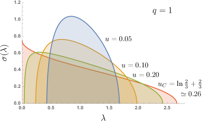
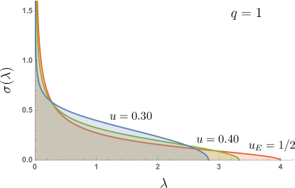
Figure 1: (Color online) Entanglement spectra $\sigma(\lambda)$ at $q=1$ for various values of the von Neumann entropy $S_{1}=\ln N-u$: entanglement decreases as $u$ increases. (a) Entangled phase: $0\leq u\leq u_{C}(1)=\ln(2/3)+2/3$, (b) Typical phase: $u_{C}(1)\leq u\leq u_{E}(1)=1/2$. Both $u_{C}(1)$ and $u_{E}(1)$ are critical values belonging to the critical lines $u_{C}(q)$ and $u_{E}(q)$, see Fig. 5.

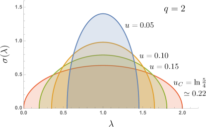
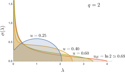
Figure 2: (Color online) Entanglement spectra $\sigma(\lambda)$ at $q=2$ for various values of (the logarithm of) purity $S_{2}=\ln N-u$: entanglement decreases as $u$ increases. (a) Entangled phase: $0\leq u\leq u_{C}(2)=\ln(5/4)$, (b) Typical phase: $u_{C}(2)\leq u\leq u_{E}(2)=\ln 2$. Both $u_{C}(2)$ and $u_{E}(2)$ are critical values belonging to the critical lines $u_{C}(q)$ and $u_{E}(q)$, see Fig. 5.

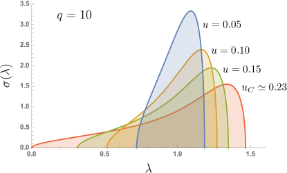
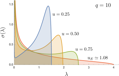
Figure 3: (Color online) Entanglement spectra $\sigma(\lambda)$ at $q=10$ for various values of the Rényi entropy $S_{10}=\ln N-u$: entanglement decreases as $u$ increases. (a) Entangled phase: $0\leq u\leq u_{C}(10)\simeq 0.23$, (b) Typical phase: $u_{C}(10)\leq u\leq u_{E}(10)\simeq 1.08$. Both $u_{C}(10)$ and $u_{E}(10)$ are critical values belonging to the critical lines $u_{C}(q)$ and $u_{E}(q)$, see Fig. 5.

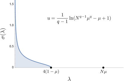
Figure 4: (Color online) Entanglement spectra $\sigma(\lambda)$ in the separable phase $u_{E}(q)<u\leq\ln N$. One eigenvalue has evaporated from the spectrum sea, which has a Marčenko-Pastur distribution.

6 The phase diagram

Some entanglement spectra are displayed in Figs. 1–4. The spectra for $q=2$ and $q=1$ were shown in Ref. [14] and [18], respectively. The spectra for a generic $q\neq 1,2$ are novel and we show an example in Fig. 3. The deformations of the spectra for different $q$ are very interesting and are easily understood by observing that large values of $q$ tend to attribute more “weight” to large eigenvalues. For any $q$, at $u=u_{E}(q)$, one eigenvalue evaporates from the spectrum sea $O(1/N)$ and becomes $O(1)$. See Fig. 4.

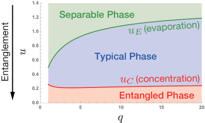
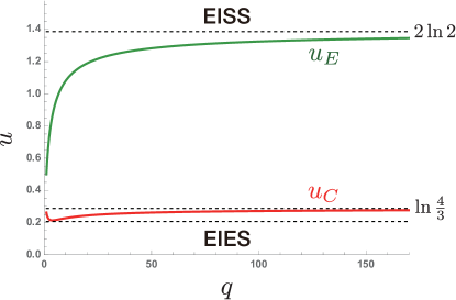
Figure 5: (Color online) Left. Phase diagram of the entanglement spectrum, ($q,u$)-plane. The entanglement $S_{q}=\ln N-u$ decreases as $u$ increases. The entangled phase (red) is for $0<u<u_{C}$: the eigenvalue distribution is a (deformed) semicircle around $1/N$; as $u\downarrow 0$ the semicircle degenerates into a Dirac delta and the state is maximally entangled. The critical line $u=u_{C}(q)$ is the “concentration” line (pushed-to-pulled transition) where the gap closes, the left endpoint of the entanglement spectrum touches the boundary $\lambda=0$ and the entanglement spectrum starts developing a sharp concentration of eigenvalues near zero; $u_{C}(q)\to\ln(4/3)$ as $q\to\infty$. The typical phase (blue) is for $u_{C}<u<u_{E}$: the critical line $u=u_{E}(q)$ is the “evaporation” line, corresponding to typical states. The largest eigenvalue evaporates from the spectrum sea, characterized by a Marčenko-Pastur distribution; $u_{E}(q)\to 2\ln 2$ as $q\to\infty$. The separable phase (green) is for $u_{E}<u<\ln N$: the line $u=\ln N$ (not shown) corresponds to separable states. Right. Same phase diagram for a wider range of $q$. Observe that $u_{C}(q)$ has a minimum $u_{C}\simeq 0.214$ at $q\simeq 3.733$. States EIES (entropy-independent entangled states) below the lowest dashed line are entangled independently of the adopted entropy measure (namely, the value of $q$). States EISS (entropy-independent separable states) above the dashed asymptote have a significant ($O(1)$) separable component independently of the adopted entropy measure (namely, the value of $q$).

As anticipated, as $q$ and $u$ are varied, one encounters two critical lines. See Fig. 5. Starting from small values of $u$ (large entanglement $S_{q}=\ln N-u$ across the bipartition), one encounters a first phase transition at $u=u_{C}(q)$. This first critical line separates an “entangled” phase (red in the figure), present for $0<u<u_{C}$, from a “typical” phase (blue in the figure).

In the entangled phase the entanglement spectrum is a (deformed) semicircle around $1/N$. Notice that as $u\downarrow 0$ the semicircle degenerates into a Dirac delta, corresponding to maximally entangled states.

Across the critical line $u=u_{C}(q)$ the so-called pushed-to-pulled transition takes place. We call it the “concentration” line, here the gap closes and the entanglement spectrum touches the boundary $\lambda=0$, so that the left endpoint $a=0$. Above this critical line a sharp concentration of eigenvalues near zero is formed with the development of a sharp (integrable) spike. Observe that $u_{C}(q)\to\ln(4/3)$ as $q\to\infty$. Along the concentration line $u=u_{C}(q)$ the phase transition is third order [14], except at $q=1$, where it becomes fourth order [18].

As $u$ increases, for $u_{C}<u<u_{E}$, one finds the typical phase. Eventually, one reaches the second critical line $u=u_{E}(q)$, which separates the typical phase from a “separable” phase (green in the figure), present for $u_{E}<u<\ln N$.

The value $u=u_{E}(q)$ is characterized by the onset of evaporation of the largest eigenvalue. For $u=u_{E}(q)$ the distribution is Marčenko-Pastur. Observe that $u_{E}(q)\to 2\ln 2$ as $q\to\infty$, and $u=\ln N$ for genuinely separable states. Along the evaporation line $u=u_{E}(q)$ the phase transition is first order [14], except at $q=1$, where it becomes second order [18]. Interestingly, at $q=1$ the phase transitions are softer.

All phase transitions are detected by a change in the entanglement spectrum. This is reflected in a sharp variation of the relative volume of the manifolds with constant entanglement (isoentropic manifolds) [14].

We observe that states above the first asymptote, at $q=2\ln 2$, always have a significant separable component $O(1)$, independently of the value of $q$, and therefore of the Rényi entropy used to measure entanglement. We call them “entropy-independent separable states” (EISS). States below the parallel line tangent to the minimum of $u_{C}(q)$ are significantly entangled, independently of the value of $q$, and therefore of the particular Rényi entropy. We call them “entropy-independent entangled states” (EIES). Further investigation is needed to understand what EISS and EIES are and if they have some sort of characterization.

7 Conclusions and perspectives

We have determined the phase diagram of the entanglement spectrum for a bipartite quantum system. The analysis hinges upon saddle point equations and a Coulomb gas method. It is valid in the limit of large quantum systems.

The present analysis basically completes the characterization of typical bipartite entanglement. Multipartite entanglement is much more difficult to study. One possible strategy consists in looking at the distribution of bipartite entanglement when the bipartition is varied [37, 38]. This problem is more difficult, and no complete characterization exists, although a number of interesting ideas have been proposed, in particular for small subsystems [39, 40, 41, 42, 43, 44]. One of the main roadblocks seems to be the presence of frustration [45], which makes the analysis (and the numerics) more involved. A thorough understanding of multipartite entanglement is however crucial, also in view of possible quantum applications [46].

References

References

- [1] M. A. Nielsen and I. L. Chuang, Quantum Computation and Quantum Information (Cambridge University Press, Cambridge, 2000).
- [2] I. Bengtsson and K. Życzkowski, Geometry of Quantum States: An Introduction to Quantum Entanglement, (Cambridge University Press, 2009)
- [3] W. K. Wootters, Entanglement of formation and concurrence, Quantum Inf. Comput. 1, 27 (2001).
- [4] L. Amico, R. Fazio, A. Osterloh, and V. Vedral, Entanglement in many-body systems, Rev. Mod. Phys. 80, 517 (2008).
- [5] R. Horodecki, P. Horodecki, M. Horodecki, and K. Horodecki, Quantum entanglement, Rev. Mod. Phys. 81, 865 (2009).
- [6] E. Lubkin, Entropy of an -system from its correlation with a -reservoir, J. Math. Phys. 19, 1028 (1978).
- [7] D. N. Page, Average entropy of a subsystem, Phys. Rev. Lett. 71, 1291 (1993).
- [8] S. K. Foong and S. Kanno, Proof of Page’s conjecture on the average entropy of a subsystem Phys. Rev. Lett. 72, 1148 (1994).
- [9] J. Sánchez-Ruiz, Simple proof of Page’s conjecture on the average entropy of a subsystem, Phys. Rev. E 52, 5653 (1995).
- [10] S. Sen, Average Entropy of a Quantum Subsystem, Phys. Rev. Lett. 77, 1 (1996).
- [11] O. Giraud, Purity distribution for bipartite random pure states, J. Phys. A: Math. Theor. 40, F1053 (2007).
- [12] P. Hayden, D. W. Leung, and A. Winter, Aspects of Generic Entanglement, Commun. Math. Phys. 265, 95 (2006).
- [13] P. Facchi, U. Marzolino, G. Parisi, S. Pascazio, and A. Scardicchio, Phase transitions of bipartite entanglement, Phys. Rev. Lett. 101, 050502 (2008).
- [14] A. De Pasquale, P. Facchi, G. Parisi, S. Pascazio, and A. Scardicchio, Phase transitions and metastability in the distribution of the bipartite entanglement of a large quantum system, Phys. Rev. A 81, 052324 (2010).
- [15] A. De Pasquale, P. Facchi, V. Giovannetti, G. Parisi, S. Pascazio, and A. Scardicchio, Statistical distribution of the local purity in a large quantum system, J. Phys. A: Math. Theor. 45, 015308 (2012).
- [16] C. Nadal, S. N. Majumdar, and M. Vergassola, Phase Transitions in the Distribution of Bipartite Entanglement of a Random Pure State, Phys. Rev. Lett. 104, 110501 (2010).
- [17] C. Nadal, S. N. Majumdar, and M. Vergassola, Statistical Distribution of Quantum Entanglement for a Random Bipartite State, J. Stat. Phys. 142, 403 (2011).
- [18] P. Facchi, G. Florio, G. Parisi, S. Pascazio, and K. Yuasa, Entropy-Driven Phase Transitions of Entanglement Physical Review A 87, 052324 (2013).
- [19] F.J. Dyson, Statistical theory of energy levels of complex systems II, J. Math. Phys. 3, 157 (1962).
- [20] P.J. Forrester, Log-Gases and Random Matrices (Princeton University Press, Princeton, 2010).
- [21] F.D. Cunden, P. Facchi, G. Florio, S. Pascazio, Typical entanglement, Eur. Phys. J. Plus 128, 48 (2013).
- [22] F.D. Cunden, P. Facchi, G. Florio, Polarized ensembles of random pure states, J. Phys. A: Math. Theor. 46, 315306 (2013).
- [23] F.D. Cunden, P. Facchi, P. Vivo, A shortcut through the Coulomb gas method for spectral linear statistics on random matrices, J. Phys. A: Math. Theor. 49, 135202 (2016).
- [24] F.D. Cunden, P. Facchi, M. Ligabò, P. Vivo, Universality of the third-order phase transition in the constrained Coulomb gas, J. Stat. Mech. Theory Exp. 2017, 053303 (2017).
- [25] J.M. Kosterlitz, D.J. Thouless, R.C. Jones, Spherical Model of a Spin-Glass, Phys. Rev. Lett. 36, 1217 (1976).
- [26] R.C. Jones, J.M. Kosterlitz, D.J. Thouless, The eigenvalue spectrum of a large symmetric random matrix with a finite mean, J. Phys. A: Math. Gen. 11, L45 (1978).
- [27] D.J. Gross, E. Witten, Possible third order phase transition in the large- lattice gauge theory, Phys. Rev. D 21, 446 (1980).
- [28] G. ’t Hooft, A planar diagram theory for strong interactions, Nucl. Phys. B 72, 461 (1974).
- [29] E. Brezin, C. Itzykson, G. Parisi, J.B. Zuber, Planar diagrams, Commun. Math. Phys. 59, 35 (1978).
- [30] S.N. Majumdar, G. Schehr, Top eigenvalue of a random matrix: large deviations and third order phase transition, J. Stat. Mech Theory Exp. 2014, P01012 (2014).
- [31] F.D. Cunden, P. Facchi, M. Ligabò, P. Vivo, Universality of the weak pushed-to-pulled transition in systems with repulsive interactions, J. Phys. A: Math. Theor. 51, 35LT01 (2018).
- [32] S. Lloyd and H. Pagels, Complexity as thermodynamic depth, Ann. Phys. (N.Y.) 188, 186 (1988).
- [33] K. Życzkowski and H.-J. Sommers, Induced measures in the space of mixed quantum states, J. Phys. A: Math. Gen. 34, 7111 (2001).
- [34] C. Itzykson and J.-B. Zuber, The planar approximation. II, J. Math. Phys. 21, 411 (1980).
- [35] V. A. Marčenko and L. A. Pastur, Distribution of eigenvalues for some sets of random matrices, Math. USSR Sb. 1, 457 (1967).
- [36] F. G. Tricomi, Integral Equations (Cambridge University Press, Cambridge, 1957).
- [37] P. Facchi, G. Florio, G. Parisi and S. Pascazio, Maximally multipartite entangled states, Physical Review A 77 (2008) 060304(R).
- [38] P. Facchi, G. Florio, U. Marzolino, G. Parisi, S. Pascazio, Classical Statistical Mechanics Approach to Multipartite Entanglement, Journal of Physics A: Mathematical and Theoretical 43 (2010) 225303
- [39] D. Goyeneche, D. Alsina, J.I. Latorre, A. Riera, K. Życzkowski, Absolutely Maximally Entangled states, combinatorial designs and multi-unitary matrices, Phys. Rev. A 92, 032316 (2015).
- [40] D. Goyeneche and K. Życzkowski, Genuinely multipartite entangled states and orthogonal arrays, Phys. Rev. A 90, 022316 (2014).
- [41] D. Goyeneche, J. Bielawski, K. Życzkowski, Multipartite entanglement in heterogeneous systems, Phys. Rev. A 94, 012346 (2016).
- [42] D. Goyeneche, Z. Raissi, S. Di Martino and K.Życzkowski, Entanglement and quantum combinatorial designs, Phys. Rev. A 97, 062326-12 (2018).
- [43] G. Gour and N. R. Wallach, All maximally entangled four-qubit states, J. Math. Phys. 51, 112201 (2010).
- [44] F. Huber, O. Gühne, J. Siewert, Absolutely maximally entangled states of seven qubits do not exist, Phys. Rev. Lett. 118, 200502 (2017).
- [45] P. Facchi, G. Florio, U. Marzolino, G. Parisi, S. Pascazio, Multipartite Entanglement and Frustration, New Journal of Physics 12, 025015 (2010).
- [46] J. Zhang, G. Adesso, C. Xie and K. Peng, Quantum Teamwork for Unconditional Multiparty Communication, Phys. Rev. Lett. 103, 070501 (2009).