On Expansions and Nodes for Sparse Grid Collocation of Lognormal Elliptic PDEs

Abstract

This work is a follow-up to our previous contribution (“Convergence of sparse collocation for functions of countably many Gaussian random variables (with application to elliptic PDEs)”, SIAM J. Numer. Anal., 2018), and contains further insights on some aspects of the solution of elliptic PDEs with lognormal diffusion coefficients using sparse grids. Specifically, we first focus on the choice of univariate interpolation rules, advocating the use of Gaussian Leja points as introduced by Narayan and Jakeman (“Adaptive Leja sparse grid constructions for stochastic collocation and high-dimensional approximation”, SIAM J. Sci. Comput., 2014) and then discuss the possible computational advantages of replacing the standard Karhunen-Loève expansion of the diffusion coefficient with the Lévy-Ciesielski expansion, motivated by theoretical work of Bachmayr, Cohen, DeVore, and Migliorati (“Sparse polynomial approximation of parametric elliptic PDEs. part II: lognormal coefficients”, ESAIM: M2AN, 2016). Our numerical results indicate that, for the problem under consideration, Gaussian Leja collocation points outperform Gauss–Hermite and Genz–Keister nodes for the sparse grid approximation and that the Karhunen–Loève expansion of the log diffusion coefficient is more appropriate than its Lévy–Ciesielski expansion for purpose of sparse grid collocation.

1 Introduction

We consider the sparse polynomial collocation method for approximating the solution of a random elliptic boundary value problem with lognormal diffusion coefficient, a well-studied model problem for uncertainty quantification in numerous physical systems such as stationary groundwater flow in an uncertain aquifer. The assumption of a lognormal diffusion coefficient, i.e., that its logarithm is a Gaussian random field, is a common, quite simple approach for modeling uncertain conductivities with large variability in practice (a discussion on this and other, more sophisticated models for the conductivity of aquifers can be found e.g. in neuman.riva.guad:trunc.power , empirical evidence for lognormality is discussed in Freeze1975 ), but already yields an interesting setting from a mathematical point of view. For instance, a lognormal diffusion coefficient introduces challenges, e.g., for stochastic Galerkin methods gittelson:logn ; sarkis:lognormal ; MuglerStarkloff2013 due to the unboundedness of the coefficient and the necessity of solving large coupled linear systems. By contrast, stochastic collocation based on sparse grids XiuHesthaven2005 ; BabuskaEtAl2010 ; NobileEtAl2008a ; NobileEtAl2008b has been established as a powerful and flexible non-intrusive approximation method in high dimensions for functions of weighted mixed Sobolev regularity. The fact that solutions of lognormal diffusion problems belong to this function class has been shown under suitable assumptions in BachmayrEtAl2015 . Based on the analysis in BachmayrEtAl2015 , we have established in ErnstEtAl2018 a dimension-independent convergence rate for sparse polynomial collocation given a mild condition on the univariate node sets. This condition is, for instance, satisfied by the classical Gauss-Hermite nodes ErnstEtAl2018 . In related work, dimension-independent convergence has also been shown for sparse grid quadrature Chen2016 .

This work is a follow-up on our previous contribution ErnstEtAl2018 and provides further discussion, insights and numerical results concerning two important design decisions for sparse polynomial collocation applied to differential equations with Gaussian random fields.

The first concerns the representation of the Gaussian random field by a series expansion. A common choice is to use the Karhunen-Loève expansion GhanemSpanos1991 of the random field. Although it represents the spectral, and thus $L^{2}$-optimal, expansion of the input field, it is not necessarily the most efficient parametrization for approximating the solution field of the equation. In particular, in BachmayrEtAl2015 ; BachmayrEtAl2018 the authors advocate using wavelet-based expansions with localized basis functions. A classical example of this type is the Lévy-Ciesielski (LC) expansion of Brownian motion or a Brownian bridge Ciesielski1961 ; BhattacharyaWaymire2016 , which employs hat functions, whereas the KL expansion of the same random fields results in sinusoidal (hence smoother and globally supported) basis functions. A theoretical advantage of localized expansions of Gaussian random fields is that for these it is easier to verify the (sufficient) condition for weighted mixed Sobolev regularity of the solution of the associated lognormal diffusion problem. In this work, we conduct numerical experiments with the KL and LC expansions of a Brownian bridge as the lognormal coefficient in an elliptic diffusion equation in order to study their relative merits for sparse grid collocation of the resulting solution. We note that finding optimal representations of the random inputs is a topic of ongoing research, see e.g. Bohn2018 ; Papaioannou2019 ; Tipireddy2014 .

The second design decision we investigate is the choice of the univariate polynomial interpolation node sequences which form the building blocks of sparse grid collocation. Established schemes are Lagrange interpolation based on Gauss–Hermite or Genz–Keister nodes. However, the former are non-nested and the latter grow rapidly in number and are only available up to a certain level. In recent work, weighted Leja nodes NarayanJakeman2014 have been advocated as a suitable nested and slowly increasing node family for sparse grid approximations, see, e.g., Loukrezis2019 ; FarcasEtAl2019 ; VanDenBosEtal2018 for recent applications in uncertainty quantification. However, so far there exist only preliminary results regarding the numerical analysis of weighted Leja points on unbounded domains, e.g., JantschEtAl2019 . We provide numerical evidence that Gaussian Leja nodes, i.e., weighted Leja nodes with Gaussian weight, satisfy as well the sufficient condition given in ErnstEtAl2018 for dimension-independent sparse polynomial collocation. Moreover, we compare the performance of sparse grid collocation based on Gaussian Leja, Gauss–Hermite and Genz–Keister nodes for the approximation of the solution of a lognormal random diffusion equation.

The remainder of the paper is organized as follows. In Section 2 we provide the necessary fundamentals on lognormal diffusion problems and discuss the classical Karhunen–Loève expansion of random fields and expansions based on wavelets. Sparse polynomial collocation using sparse grids are introduced in Section 3, where we also recall our convergence results from ErnstEtAl2018 . Moreover, we discuss the use of Gaussian Leja points for quadrature and sparse grid collocation in connection with Gaussian distributions in Section 3.2. Finally, in Section 4, we present our numerical results for sparse polynomial collocation applied to lognormal diffusion problems using the above-mentioned univariate node families and expansion variants for random fields. We draw final conclusions in Section 5.

2 Lognormal Elliptic Partial Differential Equations

We consider a random elliptic boundary value problem on a bounded domain $D\subset\mathbb{R}^{d}$ with smooth boundary $\partial D$,

$$-\nabla\cdot(a(\omega)\,\nabla u(\omega))=f\quad\text{in }D,\qquad u(\omega)=0\;\text{on }\partial D,\qquad\mathbb{P}\text{-a.s.~{},}$$ (1)

with a random diffusion coefficient $a:D\times\Omega\to\mathbb{R}$ w.r.t. an underlying probability space $(\Omega,\mathcal{A},\mathbb{P})$. If $a(\cdot,\omega)\colon D\to\mathbb{R}$ satisfies the conditions of the Lax–Milgram lemma GilbargTrudinger2001 $\mathbb{P}$-almost surely, then a pathwise solution $u:\Omega\to H_{0}^{1}(D)$ of (1) exists. Under suitable assumptions on the integrability of $a_{\min}(\omega):=\operatorname*{\operatorname{ess\,inf}}_{x\in D}a(x,\omega)$ one can show that $u$ belongs to a Lebesgue–Bochner space $L^{p}_{\mathbb{P}}(\Omega;H_{0}^{1}(D))$ consisting of all random functions $v\colon\Omega\to H_{0}^{1}(D)$ with $\|v\|_{L^{p}}:=\left(\int_{\Omega}\|v(\omega)\|^{p}_{H_{0}^{1}(D)}\ \mathbb{P}(\mathrm{d}\omega)\right)^{1/p}$.

In this paper, we consider lognormal random coefficients $a$, i.e., where $\log a\colon D\times\Omega\to\mathbb{R}$ is a Gaussian random field which is uniquely determined by its mean function $\phi_{0}\colon D\to\mathbb{R}$, $\phi_{0}(x):={\bm{\mathsf{E}}}\left[\log a(x)\right]$ and its covariance function $c\colon D\times D\to\mathbb{R}$, $c(x,x^{\prime}):=\operatorname{Cov}(\log a(x),\log a(x^{\prime}))$. If the Gaussian random field $\log a$ has continuous paths the existence of a weak solution $u\colon\Omega\to H_{0}^{1}(D)$ can be ensured.

Proposition 1 ((Charrier2012, , Section 2))

Let $\log a$ in (1) be a Gaussian random field with $a(\cdot,\omega)\in\pazocal{C}(D)$ almost surely. Then a unique solution $u\colon\Omega\to H_{0}^{1}(D)$ of (1) exists such that $u\in L^{p}_{\mathbb{P}}(\Omega;H_{0}^{1}(D))$ for any $p>0$.

A Gaussian random field $\log a\colon D\times\Omega\to\mathbb{R}$ can be represented as a series expansion of the form

$$\log a(x,\omega)=\phi_{0}(x)+\sum_{m\geq 1}\phi_{m}(x)\,\xi_{m}(\omega),\qquad\xi_{m}\sim\mathsf{N}(0,1)\text{ i.i.d.},$$ (2)

with suitably chosen $\phi_{0},\phi_{m}\in L^{\infty}(D)$, $m\geq 1$. In general, several such expansions or expansion bases $\{\phi_{m}\}_{m\in\mathbb{N}}$, respectively, can be constructed, cf. Section 2.2—thus raising the question of whether certain bases $\{\phi_{m}\}_{m\in\mathbb{N}}$ are better suited for parametrizing random fields than others. Conversely, given an appropriate system $\{\phi_{m}\}_{m\in\mathbb{N}}$, the construction (2) will yield a Gaussian random field if we ensure that the expansion in (2) converges $\mathbb{P}$-almost surely pointwise or in $L^{\infty}(D)$, i.e., that the Gaussian coefficient sequence $(\xi_{m})_{m\in\mathbb{N}}$ in $\mathbb{R}^{\mathbb{N}}$ with distribution $\mu:=\bigotimes_{m\in\mathbb{N}}N(0,1)$ satisfies

$$\mu(\Gamma)=1\quad\text{ where }\quad\Gamma:=\Bigl{\{}\bm{\xi}\in\mathbb{R}^{\mathbb{N}}:\|\sum_{m=1}^{\infty}\phi_{m}\xi_{m}\|_{L^{\infty}(D)}<\infty\Bigr{\}}.$$ (3)

We remark that $\Gamma$ is a linear subspace of $\mathbb{R}^{\mathbb{N}}$. The basic condition (3) is satisfied, for instance, if

$$\sum_{m\geq 1}\|\phi_{m}\|_{L^{\infty}(D)}<\infty$$ (4)

and (2) then yields a Gaussian random variable in $L^{\infty}(D)$, see (SchwabGittelson2011, , Lemma 2.28) or (Sprungk2017, , Section 2.2.1). Given the assumption (3) we can view the random function $a$ in (2) and the resulting pathwise solution $u$ of (1) as functions in $L^{\infty}(D)$ and $H_{0}^{1}(D)$, respectively, depending on the random parameter $\bm{\xi}\in\Gamma$, i.e., $a\colon\Gamma\to L^{\infty}(D)$ and $u\colon\Gamma\to H_{0}^{1}(D)$. In particular, by the Lax–Milgram lemma we have that $u(\bm{\xi})\in H_{0}^{1}(D)$ is well-defined for $\bm{\xi}\in\Gamma$ and

$$\|u(\bm{\xi})\|_{H_{0}^{1}(D)}\leq\frac{C_{D}}{a_{\min}(\bm{\xi})}\|f\|_{L^{2}(D)},\qquad a_{\min}(\bm{\xi}):=\operatorname*{\operatorname{ess\,inf}}_{x\in D}a(x,\bm{\xi}).$$

In the following subsection, we provide sufficient conditions on the series representation in (2) such that (3) holds and that the solution $u\colon\Gamma\to H_{0}^{1}(D)$ of (1) belongs to a Lebesgue–Bochner space $L^{p}_{\mu}(\Gamma;H_{0}^{1}(D))$. Moreover, we discuss the regularity of the solution $u$ of the random PDE (1) as a function of the variable $\bm{\xi}\in\Gamma$, which governs approximability by polynomials in $\bm{\xi}$.

2.1 Integrability and Regularity of the Solution

A first result concerning the integrability of $u$ given $\log a$ as in (2) is the following.

Proposition 2 ((SchwabGittelson2011, , Proposition 2.34))

If the functions $\phi_{m}$, $m\in\mathbb{N}$, in (2) satisfy (4), then (3) holds and the solution $u\colon\Gamma\to H_{0}^{1}(D)$ of (1) with diffusion coefficient $a$ as in (2) satisfies $u\in L^{p}_{\mu}(\Gamma;H_{0}^{1}(D))$ for any $p>0$.

In (BachmayrEtAl2015, , Corollary 2.1) the authors establish the same statements as in Proposition 2 but under the assumption that there exists a strictly positive sequence $(\tau_{m})_{m\in\mathbb{N}}$ such that

$$\sup_{x\in D}\sum_{m\geq 1}\tau_{m}|\phi_{m}(x)|<\infty,\qquad\sum_{m\geq 1}\exp(-\tau^{2}_{m})<\infty.$$ (5)

Compared with (4), this relaxes the summability condition if the functions $\phi_{m}$ have local support. On the other hand, (5) implies that $(|\phi_{m}(x)|)_{m\in\mathbb{N}}$ decays slightly faster than a general $\ell^{1}(\mathbb{N})$-sequence due to the required growth of $\tau_{m}\geq C\sqrt{\log m}$.

The authors of BachmayrEtAl2015 further establish a particular weighted Sobolev regularity of the solution $u\colon\Gamma\to H_{0}^{1}(D)$ of (1) w.r.t. $\bm{\xi}$ or $\xi_{m}$, respectively, assuming a stronger version of (5). To state their result, we introduce further notation. We define the partial derivative $\partial_{\xi_{m}}v(\bm{\xi})$ for a function $v\colon\Gamma\to H_{0}^{1}(D)$ by

$$\partial_{\xi_{m}}v(\bm{\xi}):=\lim_{h\to 0}\frac{v(\bm{\xi}+h\mathbf{e}_{m})-v(\bm{\xi})}{h},$$

when it exists, where $\mathbf{e}_{m}$ denotes the $m$-th unit vector in $\mathbb{R}^{\mathbb{N}}$. Higher derivatives $\partial^{k}_{\xi_{m}}v(\bm{\xi})$ are defined inductively. Thus, for any $k\in\mathbb{N}$ we have $\partial^{k}_{\xi_{m}}v\colon\Gamma\to H_{0}^{1}(D)$, assuming its existence on $\Gamma$. In order to denote arbitrary mixed derivatives we introduce the set

$$\mathcal{F}:=\bigl{\{}\mathbf{k}\in\mathbb{N}_{0}^{\mathbb{N}}:|\mathbf{k}|_{0}<\infty\bigr{\}},\qquad|\mathbf{k}|_{0}:=|\{m\in\mathbb{N}:k_{m}>0\}|,$$ (6)

of finitely supported multi-index sequences $\mathbf{k}\in\mathbb{N}_{0}^{\mathbb{N}}$. For $\mathbf{k}\in\mathcal{F}$ we can then define the partial derivative $\partial^{\mathbf{k}}v\colon\Gamma\to H_{0}^{1}(D)$ of a function $v\colon\Gamma\to H_{0}^{1}(D)$ by

$$\partial^{\mathbf{k}}v(\bm{\xi}):=\left(\prod_{m\geq 1}\partial^{k_{m}}_{\xi_{m}}\right)v(\bm{\xi}),$$

where the product is, in fact, finite due to the definition of $\mathcal{F}$.

Remark 1

It was shown in BachmayrEtAl2015 that the partial derivative $\partial^{\mathbf{k}}u(\bm{\xi})\in H_{0}^{1}(D)$, $\mathbf{k}\in\mathcal{F}$, of the solution $u$ of (1) can itself be characterized as the solution of a variational problem in $H_{0}^{1}(D)$:

$$\int_{D}a(\bm{\xi})\,\nabla[\partial^{\mathbf{k}}u(\bm{\xi})]\cdot\nabla v\ \mathrm{d}x=\int_{D}\sum_{\mathbf{i}\lneqq\mathbf{k}}\begin{pmatrix}\mathbf{k}\\ \mathbf{i}\end{pmatrix}\ \phi^{\mathbf{k}-\mathbf{i}}a(\bm{\xi})\nabla[\partial^{\mathbf{i}}u(\bm{\xi})]\cdot\nabla v\ \mathrm{d}x\quad\forall v\in H_{0}^{1}(D)$$

where $\mathbf{i}\lneqq\mathbf{k}$ denotes that $i_{m}\leq k_{m}$ for all $m\in\mathbb{N}$ but $\mathbf{i}\neq\mathbf{k}$ and $\phi^{\mathbf{i}}$, $\mathbf{i}\in\mathcal{F}$, is a shorthand notation for the finite product $\prod_{m\geq 1}\phi^{i_{m}}_{m}\in L^{\infty}(D)$.

We now state the regularity result in BachmayrEtAl2015 which uses a slightly stronger assumption than (5).

Theorem 2.1 ((BachmayrEtAl2015, , Theorem 4.2))

Let $r\in\mathbb{N}$ and let there exist strictly positive weights $\tau_{m}>0$, $m\in\mathbb{N}$ such that for the functions $\phi_{m}$, $m\in\mathbb{N}$, in (2) and for a $p>0$ we have

$$\sup_{x\in D}\sum_{m\geq 1}\tau_{m}|\phi_{m}(x)|<\frac{\log 2}{\sqrt{r}}\qquad\sum_{m\geq 1}\tau^{-p}_{m}<\infty.$$ (7)

Then the solution $u\colon\Gamma\to H_{0}^{1}(D)$ of (1) with coefficient a as in (2) satisfies

$$\sum_{\begin{subarray}{c}\mathbf{k}\in\mathcal{F},\\ |\mathbf{k}|_{\infty}\leq r\end{subarray}}\frac{\bm{\tau}^{2\mathbf{k}}}{\mathbf{k}!}\|\partial^{\mathbf{k}}u\|^{2}_{L^{2}_{\mu}}<\infty,\quad\text{ where }\bm{\tau}^{\mathbf{k}}=\prod_{m\geq 1}\tau_{m}^{k_{m}}\text{ and }\mathbf{k}!=\prod_{m\geq 1}k_{m}!~{}.$$ (8)

This theorem tells us that, given (7), the partial derivatives $\partial^{\mathbf{k}}u\colon\Gamma\to H_{0}^{1}(D)$ exist for any $\mathbf{k}\in\mathcal{F}$ with $|\mathbf{k}|_{\infty}<\infty$ and belong to $L^{2}_{\mu}(\Gamma;H_{0}^{1}(D))$. Moreover, their $L^{2}_{\mu}$-norm decays faster than $\bm{\tau}^{-2\mathbf{k}}$—otherwise (8) would not hold. In particular, Theorem 2.1 establishes a weighted mixed Sobolev regularity of the solution $u\colon\Gamma\to H_{0}^{1}(D)$ of maximal degree $r\in\mathbb{N}$ and with increasing weights $\tau_{m}\geq Cm^{1/p}$. As it turns out, it is such a regularity which ensures dimension-independent convergence rates for polynomial sparse grid collocation approximations—see the next section.

Moreover, the condition (7) seems to favor localized basis functions $\phi_{m}$ for which $\sum_{m=1}^{\infty}\tau_{m}|\phi_{m}(x)|$ reduces to a summation over a subsequence $\sum_{k=1}^{\infty}\tau_{m_{k}}|\phi_{m_{k}}(x)|$ such that (7) is easier to verify. In view of this, the authors of BachmayrEtAl2015 ; BachmayrEtAl2018 proposed using wavelet-based expansions for Gaussian random fields with sufficiently localized $\phi_{m}$ in place of the globally supported eigenmodes $\phi_{m}$ in the Karhunen–Loève (KL) expansion. In fact, condition (7) fails to hold for the KL expansion of some rough Gaussian processes (Example 1 below), but can be established if the process is sufficiently smooth (Example 2). We will discuss KL and wavelet-based expansions of Gaussian processes in more detail in the next subsection.

2.2 Choice of Expansion Bases

Given a Gaussian random field $\log a\colon D\times\Omega\to\mathbb{R}$ with mean $\phi_{0}\colon D\to\mathbb{R}$ and covariance function $c\colon D\times D\to\mathbb{R}$ we seek a representation as an expansion (2). We explain in the following how such expansions can be derived in general. To this end, we assume that the random field has $\mathbb{P}$-almost surely continuous paths, i.e., $\log a\colon\Omega\to\pazocal{C}(D)$, and a continuous covariance function $c\in\pazocal{C}(D\times D)$. Thus, we can view $\log a$ also as a Gaussian random variable with values in the separable Banach space $\pazocal{C}(D)$ or, by continuous embedding, with values in the separable Hilbert space $L^{2}(D)$. The covariance operator $C\colon L^{2}(D)\to L^{2}(D)$ of the random variable $\log a\colon\Omega\to L^{2}(D)$ is then given by $(Cf)(x):=\int_{D}c(x,y)\ f(y)\ \mathrm{d}y$. This operator is of trace class and induces a dense subspace $\mathcal{H}_{C}:=\mathrm{range}\ C^{1/2}\subset L^{2}(D)$, which equipped with the inner product $\langle u,v\rangle_{C}:=\langle C^{-1/2}u,C^{-1/2}v\rangle_{L^{2}(D)}$, forms again a Hilbert space, called the Cameron–Martin space (CMS) of $\log a$. The CMS plays a crucial role for series representations (2) of $\log a$. Specifically, it is shown in LuschgyPages2009 that (2) holds almost surely in $C(D)$ if and only if the system $\{\phi_{m}\}_{m\in\mathbb{N}}$ is a so-called Parseval frame or (super) tight frame in the CMS of $\log a$, i.e., if $\{\phi_{m}\}_{m\in\mathbb{N}}\subset\mathcal{H}_{C}$ and

$$\sum_{m\geq 1}\left|\langle\phi_{m},f\rangle_{C}\right|^{2}=\|f\|^{2}_{C}\qquad\forall f\in\mathcal{H}_{C}.$$

We discuss two common choices for such frames below.

Karhunen–Loève expansions.

This expansion is based on the eigensystem $(\lambda_{m},\psi_{m})_{m\in\mathbb{N}}$ of the compact and self-adjoint covariance operator $C\colon L^{2}(D)\to L^{2}(D)$ of $\log a$. Thus, let $\psi_{m}\in L^{2}(D)$ satisfy $C\psi_{m}=\lambda_{m}\psi_{m}$ with $\lambda_{m}>0$. Since the covariance function $c$ is a continuous function on $D\times D$, we have $\psi_{m}\in\pazocal{C}(D)$ and (2) holds almost surely in $\pazocal{C}(D)$ with $\phi_{m}:=\lambda^{-1/2}_{m}\psi_{m}$, because $\{\phi_{m}\}_{m\in\mathbb{N}}\subset\mathcal{H}_{C}$ is a complete orthonormal system (CONS) of $\mathcal{H}_{C}$. In fact, the KL basis $\{\phi_{m}\}_{m\in\mathbb{N}}$ represents the only CONS of $\mathcal{H}_{C}$ that is also $L^{2}(D)$-orthogonal. In addition, as the spectral expansion of $\log a$ in $L^{2}_{\mathbb{P}}(L^{2}(D))$, it is the optimal basis in this space in the sense that the truncation error after $M$ terms $\|\log a-\phi_{0}-\sum_{m=1}^{M}\phi_{m}\xi_{m}\|_{L^{2}_{\mathbb{P}}(L^{2}(D))}$ is the smallest among all truncated expansions of length $M$ of the form

$$\log a(x,\omega)=\phi_{0}(x)+\sum_{m=1}^{M}\tilde{\phi}_{m}(x)\tilde{\xi}_{m}(\omega).$$

Under additional assumptions the KL expansion also yields optimal rates of the truncation error in $L^{2}_{\mathbb{P}}(\pazocal{C}(D))$, see again LuschgyPages2009 . However, the KL modes $\phi_{m}$ typically have global support on $D$, which often makes it difficult to verify a condition like (7). Nonetheless, for particular covariance functions, such as the Matérn kernels, bounds on the norms $\|\phi_{m}\|_{L^{\infty}(D)}$ are known, see, e.g., GrahamEtAl2015 .

Wavelet-based expansions.

We now consider expansions in orthonormal wavelet bases $\{\psi_{m}\}_{m\in\mathbb{N}}$ of $L^{2}(D)$. Given a factorization $C=SS^{*}$, $S\colon L^{2}(D)\to L^{2}(D)$, of the covariance operator $C$ (e.g., $S=S^{*}=C^{1/2}$), we can set $\phi_{m}:=S\psi_{m}$ and obtain a CONS $\{\phi_{m}\}_{m\in\mathbb{N}}$ of the CMS $\mathcal{H}_{C}$, see LuschgyPages2009 . Thus, (2) holds almost surely in $\pazocal{C}(D)$ with $\phi_{m}=S\psi_{m}$. The advantage of wavelet-based expansions is that the resulting $\phi_{m}$ often inherit the localized behavior of the underlying $\psi_{m}$, cf. Example 1, which then facilitates verification of the sufficient condition (7) for the weighted Sobolev regularity of the solution $u$ of (1). For instance, we refer to BachmayrEtAl2018 for Meyer wavelet-based expansions of Gaussian random fields with Matérn covariance functions satisfying (7). There, the authors use a periodization approach and construct the $\phi_{m}$ via their Fourier transforms. Further work on constructing and analyzing wavelet-based expansions of Gaussian random fields includes, e.g., ElliottMajda1994 ; ElliottEtAl1997 ; BenassiEtAl1997 .

Example 1 (Brownian bridge)

A simple but useful example is the standard Brownian bridge $B\colon D\times\Omega\to\mathbb{R}$ on $D=[0,1]$. This is a Gaussian process with mean $\phi_{0}\equiv 0$ and covariance function $c(x,x^{\prime})=\min(x,x^{\prime})-xx^{\prime}$. The associated CMS is given by $\mathcal{H}_{C}=H_{0}^{1}(D)$ with $\langle u,v\rangle_{C}=\langle\nabla u,\nabla v\rangle_{L^{2}(D)}$ and we have $C=SS^{*}$ with

$$Sf(x):=\int_{0}^{1}\left(\mathbf{1}_{[0,x]}(y)-x\right)f(y)\,\mathrm{d}y,\qquad f\in L^{2}(D).$$

The KL expansion of the Brownian bridge is given by

$$B(x,\omega)=\sum_{m\geq 1}\frac{\sqrt{2}}{\pi m}\sin(\pi mx)\xi(\omega),\qquad\xi_{m}\sim\mathsf{N}(0,1)\text{ i.i.d.~{},}$$ (9)

i.e., we have $\phi_{m}(x)=\frac{\sqrt{2}}{\pi m}\sin(\pi mx)$ and $\|\phi_{m}\|_{L^{\infty}(D)}=\frac{\sqrt{2}}{\pi m}$. Although the functions $\phi_{m}$ do not satisfy the assumptions of Proposition 2, existence and integrability of the solution $u$ of (1) for $\log a=B$ is guaranteed by Proposition 1, since $B$ has almost surely continuous paths. Concerning the condition (7) it can be shown that $\sum_{m\geq 1}\tau_{m}|\phi_{m}(x)|$ converges pointwise to a (discontinuous) function if $\tau_{m}\in o(m^{-1})$, i.e., $(\tau_{m}^{-1})_{m\in\mathbb{N}}\in\ell^{p}(\mathbb{N})$ only for a $p>1$, see the Appendix. However, this function turns out to be unbounded in a neighborhood of $x=0$ if $(\tau_{m}^{-1})_{m\in\mathbb{N}}\in\ell^{p}(\mathbb{N})$ for $p\leq 2$, and numerical evidence suggests that it is also unbounded if $(\tau_{m}^{-1})_{m\in\mathbb{N}}\in\ell^{p}(\mathbb{N})$ for $p>2$, again see the Appendix. Thus, the KL expansion of the Brownian bridge does not satisfy the conditions of Theorem 2.1 for the weighted Sobolev regularity of $u\colon\Gamma\to H_{0}^{1}(D)$.

Another classical series representation of the Brownian bridge is the Lévy–Ciesielski expansion Ciesielski1961 . This wavelet-based expansions uses the Haar wavelets $\psi_{m}(x)=2^{\ell/2}\psi(2^{\ell}x-j)$ where $\psi(x)=\textbf{1}_{[0,1/2]}(x)-\textbf{1}_{(1/2,1]}(x)$ is the mother wavelet and $m=2^{\ell}+j$ for level $\ell\geq 0$ and shift $j=0,\ldots,2^{\ell}-1$. Since the Haar wavelets form a CONS of $L^{2}(D)$ we obtain a Parseval frame of the CMS of the Brownian bridge by taking $\phi_{m}=S\psi_{m}$, which yields a Schauder basis consisting of the hat functions

$$\phi_{m}(x):=2^{-\ell/2}\phi(2^{\ell}x-j),\quad\phi(x):=\max(0,1-|2x-1|),\quad m=2^{\ell}+j,$$ (10)

with $j=0,\ldots,2^{\ell}-1$ and $\ell\geq 0$. Hence, for $\log a=B$ the series representation (2) also holds almost surely in $\pazocal{C}(D)$with $\phi_{m}$ as in (10), see also (BhattacharyaWaymire2016, , Section IX.1). Moreover, we have $\|\phi_{m}\|_{L^{\infty}}=2^{-\lfloor\log_{2}m\rfloor/2}$, resulting in $\sum_{m\geq 1}\|\phi_{m}\|_{L^{\infty}}=\infty$. On the other hand, due to the localization of $\phi_{m}$ we have that for any fixed $x\in D$ and each level $\ell\geq 0$ there exists only one $k_{\ell}\in\{0,\ldots,2^{\ell}-1\}$ such that $\phi_{2^{\ell}+k_{\ell}}(x)\neq 0$. In particular, it can be shown that the LC expansion of the Brownian bridge satisfies the conditions of Theorem 2.1 for any $p>2$, since for $\tau_{m}=\kappa^{\lfloor\log_{2}m\rfloor}$ with $|\kappa|<\sqrt{2}$ we get

$$\sum_{m\geq 1}\kappa^{\lfloor\log_{2}m\rfloor}|\phi_{m}(x)|=\sum_{l\geq 0}\kappa^{\ell/2}|\phi_{2^{\ell}+k_{\ell}}(x)|\leq\sum_{l\geq 0}(\sqrt{0.5}\rho)^{\ell}<\infty$$

and for $p>\log_{\kappa}2>2$

$$\sum_{m\geq 1}\tau_{m}^{-p}=\sum_{l\geq 0}2^{l}\kappa^{-\ell p}=\sum_{l\geq 0}\left(2\kappa^{-p}\right)^{\ell}<\infty.$$

Example 2 (Smoothed Brownian bridge)

Based on the explicit KL expansion of the Brownian bridge we can construct Gaussian random fields with smoother realizations by

$$B_{q}(x,\omega)=\sum_{m\geq 1}\frac{\sqrt{2}}{(\pi m)^{q}}\sin(\pi mx)\xi(\omega),\qquad\xi_{m}\sim\mathsf{N}(0,1)\text{ i.i.d.~{},}\quad q>1.$$ (11)

Now, the resulting $\phi_{m}=\frac{\sqrt{2}}{(\pi m)^{q}}\sin(\pi m\cdot)$ indeed satisfy the assumptions of Proposition 2 for any $q>1$, since $\|\phi_{m}\|_{L^{\infty}(D)}\propto m^{-q}$. Moreover, for $p>\frac{1}{q-1}$ the expansion (11) satisfies the assumptions of Theorem 2.1 with $\tau_{m}=m^{(1+\epsilon)/p}$ for sufficiently small $\epsilon$. For this Gaussian random field $B_{q}$ the covariance function is given by $c(x,y)=2\sum_{m\geq 1}(\pi m)^{-2q}\sin(\pi mx)\sin(\pi my)$ and we can express $C^{1/2}$ via

$$C^{1/2}f(x)=\int_{D}k(x,y)\ f(y)\ \mathrm{d}y,\qquad k(x,y)=2\sum_{m\geq 1}(\pi m)^{-q}\sin(\pi mx)\sin(\pi my).$$

Thus, we could construct alternative expansion bases for $B_{q}$ via $\phi_{m}=C^{1/2}\psi_{m}$ given a wavelet CONS $\{\psi_{m}\}_{m\in\mathbb{N}}$ of $L^{2}(D)$. However, in this case the resulting $\phi_{m}$ do not necessarily have a localized support. For instance, when taking Haar wavelets $\psi_{m}$ the $C^{1/2}\psi_{m}$ have global support in $D=[0,1]$, see Fig. 1.

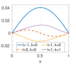
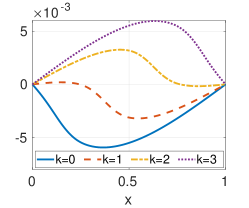
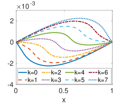
Figure 1: Expansion functions resulting from applying $C^{1/2}$ as in Example 2 for $q=3$ to the Haar wavelets $\psi_{m}$, $m=2^{\ell}+k$, with level $\ell\in\{-1,0,1\}$ (left), $\ell=2$ (middle), and $\ell=3$ (right).

3 Sparse Grid Approximation

In ErnstEtAl2018 we presented a solution approach for solving random elliptic PDEs based on sparse polynomial collocation derived from tensorized interpolation at Gauss-Hermite nodes. The problem is cast as that of approximating the solution $u$ of (1) as a function $u:\Gamma\to H_{0}^{1}(D)$ by solving for realizations of $u$ associated with judiciously chosen collocation points $\{\bm{\xi}_{j}\}_{j=1}^{N}\subset\Gamma$.

Sparse polynomial collocation operators are constructed by tensorizing univariate Lagrange interpolation sequences $(U_{k})_{k\in\mathbb{N}_{0}}$ defined as

$$(U_{k}f)(\xi)=\sum_{i=0}^{k}f(\xi_{i}^{(k)})\,L_{i}^{(k)}(\xi),\qquad f\colon\mathbb{R}\to\mathbb{R},$$ (12)

where $\{L_{i}^{(k)}\}_{i=0}^{k}$ denote the Lagrange fundamental polynomials of degree $k$ associated with a set of $k+1$ distinct interpolation nodes $\Xi^{(k)}:=\bigl{\{}\xi_{0}^{(k)},\xi_{1}^{(k)},\dots,\xi_{k}^{(k)}\bigr{\}}\subset\mathbb{R}$ and $L_{0}\equiv 1$. For any $\mathbf{k}\in\mathcal{F}$ (cf. (6)), the associated tensorized Lagrange interpolation operator $U_{\mathbf{k}}:=\bigotimes_{m\in\mathbb{N}}U_{k_{m}}$ is given by

$$(U_{\mathbf{k}}f)(\bm{\xi})=\left(\bigotimes_{m\in\mathbb{N}}U_{k_{m}}f\right)(\bm{\xi})=\sum_{\mathbf{i}\leq\mathbf{k}}f(\bm{\xi}_{\mathbf{i}}^{(\mathbf{k})})L_{\mathbf{i}}^{(\mathbf{k})}(\bm{\xi}),\qquad f:\mathbb{R}^{\mathbb{N}}\to\mathbb{R},$$ (13)

in terms of the tensorized Lagrange polynomials $L_{\mathbf{i}}^{(\mathbf{k})}(\bm{\xi}):=\prod_{m\in\mathbb{N}}L_{i_{m}}^{(k_{m})}(\xi_{m})$ with multivariate interpolation nodes $\bm{\xi}_{\mathbf{i}}^{(\mathbf{k})}\in\Xi^{(\mathbf{k})}:=\bigtimes_{m\in\mathbb{N}}\Xi^{(k_{m})}$. We thus have $U_{\mathbf{k}}:\mathbb{R}^{\Gamma}\to\mathcal{Q}_{\mathbf{k}}$, where

$$\mathcal{Q}_{\mathbf{k}}:=\mathrm{span}\{\bm{\xi}^{\mathbf{i}}:0\leq i_{m}\leq k_{m},m\in\mathbb{N}\},\qquad\mathbf{k}\in\mathcal{F},$$

denotes the multivariate tensor-product polynomial space of maximal degree $k_{m}$ in the $m$-th variable in the countable set of variables $\bm{\xi}=(\xi_{m})\in\mathbb{R}^{\mathbb{N}}$.

Sparse polynomial spaces can be constructed by tensorizing the univariate detail operators

$$\Delta_{k}:=U_{k}-U_{k-1},\quad k\geq 0,\qquad U_{-1}:\equiv 0,$$ (14)

giving

$$\Delta_{\mathbf{k}}:=\bigotimes_{m\in\mathbb{N}}\Delta_{k_{m}}\colon\mathbb{R}^{\Gamma}\to\mathcal{Q}_{\mathbf{k}}.$$

A sparse polynomial collocation operator is then obtained by fixing a suitable set of multi-indices $\Lambda\subset\mathcal{F}$ and setting

$$U_{\Lambda}:=\sum_{\mathbf{i}\in\Lambda}\Delta_{\mathbf{i}}:\mathbb{R}^{\Gamma}\to\mathcal{P}_{\Lambda},\qquad\text{ where }\mathcal{P}_{\Lambda}:=\sum_{\mathbf{i}\in\Lambda}\mathcal{Q}_{\mathbf{i}}.$$ (15)

It is shown in ErnstEtAl2018 that if $\Lambda$ is finite and monotone (meaning that $\mathbf{i}\in\Lambda$ implies that any $\mathbf{j}\in\mathcal{F}$ for which $\mathbf{j}\leq\mathbf{i}$ holds componentwise also belongs to $\Lambda$), then $U_{\Lambda}$ is the identity on $\mathcal{P}_{\Lambda}$ and $\Delta_{\mathbf{i}}$ vanishes on $\mathcal{P}_{\Lambda}$ for any $\mathbf{i}\not\in\Lambda$.

The construction of $U_{\Lambda}f$ for $f\colon\Gamma\to\mathbb{R}$ consists of a linear combination of tensor product interpolation operators requiring the evaluation of $f$ at certain multivariate nodes. It can be shown that for $\mathbf{i}\in\mathcal{F}$ the detail operators have the representation

$$\Delta_{\mathbf{i}}f=\Big{[}\bigotimes_{m\geq 1}(U_{i_{m}}-U_{i_{m}-1})\Big{]}f=\sum_{\mathbf{i}-\bm{1}\leq\mathbf{k}\leq\mathbf{i}}(-1)^{|\mathbf{i}-\mathbf{k}|_{1}}\Big{[}\bigotimes_{m\geq 1}U_{k_{m}}\Big{]}f,$$

leading to an alternative representation of $U_{\Lambda}$ for monotone finite subsets $\Lambda\subset\mathcal{F}$ known as the combination technique:

$$U_{\Lambda}=\sum_{\mathbf{i}\in\Lambda}c(\mathbf{i};\Lambda)\,U_{\mathbf{i}},\qquad c(\mathbf{i};\Lambda):=\sum_{\mathbf{e}\in\{0,1\}^{\mathbb{N}}\colon\mathbf{i}+\mathbf{e}\in\Lambda}(-1)^{|\mathbf{e}|_{1}}.$$ (16)

We refer to the collection of nodes appearing in the tensor product interpolants $U_{\mathbf{i}}$ as the sparse grid $\Xi_{\Lambda}\subset\Gamma$ associated with $\Lambda$:

$$\Xi_{\Lambda}=\bigcup_{\mathbf{i}\in\Lambda}\Xi^{(\mathbf{i})}.$$ (17)

In the same way, when approximating the solution $u:\Gamma\to H_{0}^{1}(D)$ of (1) by $u(\bm{\xi})\approx(U_{\Lambda}u)(\bm{\xi})$, each evaluation $u(\bm{\xi}_{j})$ at a sparse grid point $\bm{\xi}_{j}\in\Xi_{\Lambda}$ represents the solution of the PDE for the coefficient $a=a(\bm{\xi}_{j})$.

Remark 2

Let us provide some further comments.

1. The univariate interpolation operators $U_{k}$ in (12), on which the sparse grid collocation construction is based, will have degree of exactness $k$, as the associated sets of interpolation nodes $\Xi^{(k)}$ have cardinality $k+1$. Although we do not consider this here, allowing nodal sets to grow faster than this may bring some advantages. Such an example is the sequence of Clenshaw–Curtis nodes (cf. NobileEtAl2008a ), for which $|\Xi^{(0)}|=1$ and $|\Xi^{(k)}|=1+2^{k}$.

2. The Clenshaw–Curtis doubling scheme generates nested node sets $\Xi^{(k+1)}\subset\Xi^{(k)}$. This has the advantage that higher order collocation approximations may re-use function evaluations of previously computed lower-order approximations. Moreover, it was shown in BarthelmannEtAl2000 that sparse grid collocation based on nested node sequences are interpolatory. By contrast, the sequence of Gauss–Hermite nodes with $|\Xi^{(k)}|=k+1$ results in disjoint consecutive nodal sets. The number of new nodes added by each consecutive set is referred to as the granularity of the node sequence.

3. Two heuristic approaches for constructing monotone multi-index sets $\Lambda$ for sparse polynomial collocation for lognormal random diffusion equations are presented in ErnstEtAl2018 . Further details are given in Section 4.

In ErnstEtAl2018 , a convergence theory for sparse polynomial collocation approximations $f\approx U_{\Lambda}f$ of functions in $f\in L^{2}_{\mu}(\Gamma,H_{0}^{1}(D))$ was given based on the expansion

$$f(\bm{\xi})=\sum_{\mathbf{k}\in\mathcal{F}}f_{\mathbf{k}}\,H_{\mathbf{k}}(\bm{\xi}),\qquad f_{\mathbf{k}}=\int_{\Gamma}f(\bm{\xi})H_{\mathbf{k}}(\bm{\xi})\mu(\mathrm{d}\bm{\xi}),$$

in tensorized Hermite polynomials $H_{\mathbf{k}}(\bm{\xi})=\prod_{m\in\mathbb{N}}H_{k_{m}}(\xi_{m})$, $\mathbf{k}\in\mathcal{F}$, with $H_{k_{m}}$ denoting the univariate Hermite orthogonal polynomial of degree $k_{m}$, which are known to form an orthonormal basis of $L^{2}_{\mu}(\Gamma;H_{0}^{1}(D))$.

Under assumptions to be detailed below, it was shown (ErnstEtAl2018, , Theorem 3.12) that there exists a nested sequence of monotone multi-index sets $\Lambda_{N}\subset\mathcal{F}$, where $N=|\Lambda_{N}|$, such that the sparse grid collocation error of the approximation $U_{\Lambda_{N}}f$ satisfies

$$\left\|f-U_{\Lambda_{N}}f\right\|_{L^{2}_{\mu}}\leq C(1+N)^{-\left(\frac{1}{p}-\frac{1}{2}\right)},$$ (18)

for certain values of $p\in(0,2)$ with a constant $C$. The precise assumptions under which (18) was shown to hold are as follows:

1. The condition $\mu(\Gamma)=1$ on the domain of $f$ (cf. (3)).

2. An assumption of weighted $L^{2}_{\mu}$-summability on the derivatives of $f$: specifically, there exists $r\in\mathbb{N}_{0}$ such that $\partial^{\mathbf{k}}f\in L^{2}_{\mu}(\mathbb{R}^{\mathbb{N}};H_{0}^{1}(D))$ for all $\mathbf{k}\in\mathcal{F}$ with $|\mathbf{k}|_{\infty}\leq r$ and a sequence of positive numbers $(\tau_{m}^{-1})_{m\in\mathbb{N}}\in\ell^{p}(\mathbb{N})$, $p\in(0,2)$, such that relation (8) holds.

3. An assumption on the univariate sequence of interpolation nodes: there exist constants $\theta\geq 0$ and $c\geq 1$ such that the univariate detail operators (14) satisfy

   $$\max_{i\in\mathbb{N}_{0}}\|\Delta_{i}H_{k}\|_{L^{2}_{\mu}}\leq(1+ck)^{\theta},\qquad k\in\mathbb{N}_{0}.$$ (19)

In order for (18) to hold true, it is sufficient that (8) be satisfied for $r>2(\theta+1)+\frac{2}{p}$. It was shown in (ErnstEtAl2018, , Lemma 3.13) that (19) holds with $\theta=1$ for the detail operators $\Delta_{k}=U_{k}-U_{k-1}$ associated with univariate Lagrange interpolation operators $U_{k}$ at Gauss-Hermite nodes, i.e., the zeros of the univariate Hermite polynomial of degree $k+1$.

3.1 Gaussian Leja Nodes

Leja points for interpolation on a bounded interval $I\subset\mathbb{R}$ are defined recursively by fixing an arbitrary initial point $\xi_{0}\in I$ and setting

$$\xi_{k+1}:=\operatorname*{arg\,max}_{\xi\in I}\prod_{i=1}^{k}|\xi-\xi_{i}|,\qquad k\in\mathbb{N}_{0}.$$ (20)

They are seen to be nested, possessing the lowest possible granularity and have been shown to have an asymptotically optimal distribution (SaffTotik1997, , Chapter 5). The quantity maximized in the extremal problem (20) is not finite for unbounded sets $I$, which arise, e.g., when an interpolation problem is posed on the entire real line. Such is the case with parameter variables $\xi_{m}$ which follow a Gaussian distribution. By adding a weight function vanishing at infinity faster than polynomials grow, one can generalize the Leja construction to unbounded domains (cf. Lubinsky2007 ). Different ways of incorporating weights in (20) have also been proposed in the bounded case, cf. e.g. (SaffTotik1997, , p. 258), BaglamaEtAl1998 , and DeMarchi2004 . In NarayanJakeman2014 , it was shown that for weighted Leja sequences generated on unbounded intervals $I$ by solving the extremal problem

$$\xi_{k+1}=\operatorname*{arg\,max}_{\xi\in I}\sqrt{\rho(\xi)}\prod_{i=0}^{k}|\xi-\xi_{i}|,$$ (21)

where $\rho$ is a probability density function on $I$, their asymptotic distribution coincides with the probability distribution associated with $\rho$. This is shown in NarayanJakeman2014 for the generalized Hermite, generalized Laguerre and Jacobi weights, corresponding to a generalized Gaussian, Gamma and Beta distributions. Subsequently, the result of TaylorTotik2010 on the subexponential growth of the Lebesgue constant of bounded unweighted Leja sequences was generalized to the unbounded weighted case in JantschEtAl2019 .

If we choose $\rho(\xi)=\exp(-\xi^{2}/2)$ and $I=\mathbb{R}$ in (21) and set $\xi_{0}=0$, then we shall refer to the resulting weighted Leja nodes also Gaussian Leja nodes in view of their asymptotic distribution. Unfortunately, the result in JantschEtAl2019 does not imply a bound like (19) for univariate interpolation using Gaussian Leja nodes. However, we provide numerical evidence in Figure 2 suggesting that (19) is also satisfied for Gaussian Leja nodes with $\theta=1$.

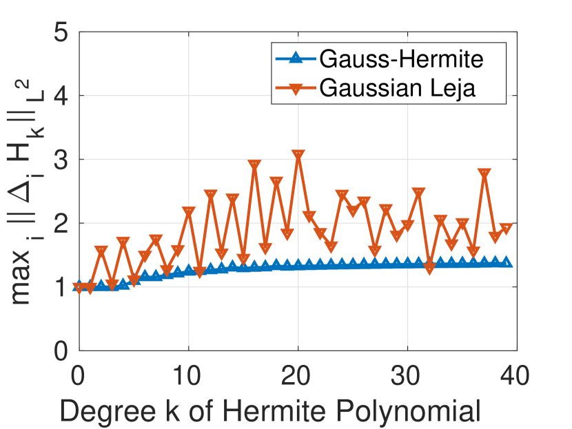
Figure 2: Comparison of $\max_{i}\|\Delta_{i}H_{k}\|_{L^{2}_{\mu}}$, $k=1,\ldots,39$, for Gauss–Hermite and Gaussian Leja nodes.

a

In the next subsection we compare the performance of Gaussian Leja nodes for quadrature and interpolation purposes to that of Gauss–Hermite and Genz–Keister nodes GenzKeister1996 , which represent another common univariate node family for quadrature w.r.t. a Gaussian weight. Although a comparison of Gaussian Leja with Genz–Keister points is already available in NarayanJakeman2014 and a comparison between Gauss–Hermite and Genz–Keister points is reported in NobileEtAl2016 ; Chen2016 , the joint comparison of the three choices has not been reported in literature to the best of our knowledge.

3.2 Performance Comparison of Common Univariate Nodes

In this section we investigate and compare the performance of numerical quadrature and interpolation of uni- and multivariate functions ($M=2,6,9$ variables) using either Gauss–Hermite, Genz–Keister or Gaussian Leja nodes. As a measure of performance we consider the achieved error in relation to the number of employed quadrature or interpolation nodes, respectively. Quadrature is carried out with respect to a standard (multivariate) Gaussian measure $\mu$ and the interpolation error is measured in $L^{2}_{\mu}$. The functions we consider in this section were previously proposed in Tamellini2012 for the purpose of comparing univariate quadrature with Gauss–Hermite and Genz–Keister points and are included in the figures displaying the results.

Quadrature results are reported in Figure 3. In the univariate case, Gauss–Hermite nodes perform best, and Genz–Keister nodes also show good performance, which is not surprising given that they are constructed as nested extensions of the Gauss–Hermite points with maximal degree of exactness. The Gaussian Leja nodes, by comparison, perform poorly. This should not surprise, however, given that Gaussian Leja points are determined by minimizing Lebesgue constants, i.e., they are conceived as interpolation points rather than quadrature points.

In the multivariate case, however, the situation changes and Gauss–Hermite nodes are the worst performing. This is due to their non-nestedness, which tends to introduce unnecessary quadrature nodes into the quadrature scheme. Note that in this case we are simply using the standard Smolyak sparse multi-index set in $M$ dimensions in Equation (15),

$$\Lambda_{w}=\biggl{\{}\mathbf{i}\in\mathbb{N}^{M}:\sum_{m=1}^{M}i_{m}\leq w\biggr{\}},\quad\mbox{for some }w\in\mathbb{N},$$

i.e., we are not tailoring the sparse grid either to the function to be integrated nor to the univariate points. The Gaussian Leja and Genz–Keister points show a faster decay of the quadrature error, due to their nestedness. This is remarkable in particular for Gaussian–Leja, given that they were proposed in literature as univariate interpolation points, as already discussed. Overall, the Genz–Keister points show the best performance as expected, but it is important to recall that only a limited number of Genz–Keister nodes is available, i.e., no nested Genz–Keister quadrature formula with real quadrature weights and more than 35 nodes is known in literature, GenzKeister1996 ; Tamellini2012 ; heiss.winschel:kpnquad . In particular, the plots report the largest standard sparse grids that can be built with these rules before running out of tabulated Genz–Keister points.

We remark that introducing a Genz–Keister quadrature formula with more than 35 nodes is not a simple matter of investing more computational effort and tabulating more points, but it would entail some “trial and error” phase to look for a suitable sequence of so-called “generators”, see e.g. Tamellini2012 for more details. This activity exceeds the scope of this paper. Moreover, Genz–Keister nodes are significantly less granular, which could be a disadvantage in certain situations: indeed, the cardinalities of the univariate Genz–Keister node sets are $|\Xi^{(k)}|=1,3,9,19,35$ for $k=0,\dots,4$ (and a sequence of Genz–Keister sets exceeding $35$ nodes might be even less granular, e.g., jumping from 1 to 5 or 7).

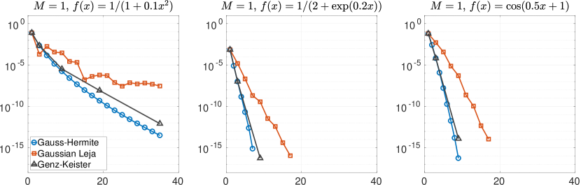
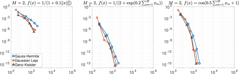
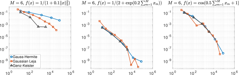
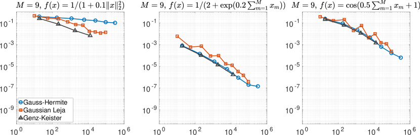
Figure 3: Results for univariate and multivariate quadrature test.

Next, we turn to comparing the performance of the different node families for interpolation. Here, Gaussian Leja nodes are expected to be best (or close-to-best) performing, given their specific design. Measuring interpolation error on unbounded domains with a Gaussian measure (or any non-uniform measure for that matter) is a delicate task, as one would need to choose a proper weight to ensure boundedness of the pointwise error, see e.g. Harbrecht2016 ; NobileEtAl2016 . In this contribution, we actually discuss the $L^{2}_{\mu}$ approximation error of the interpolant, which we compute as follows: we sample $K$ independent batches of $M$-variate Gaussian random variables, with $P$ points each, $\mathcal{B}_{k}=\{\bm{\xi}_{i}\}_{i=1}^{P},\xi_{i,m}\sim\mathsf{N}(0,1),m=1,\ldots,M,k=1,\ldots,K$; we construct a sequence of increasingly accurate sparse grids $U_{\Lambda_{w}}[f]$ and evaluate them on each random batch; we then approximate the $L^{2}_{\mu}$ error for each sparse grid on each batch by Monte Carlo,

$$\text{Err}_{k}(U_{\Lambda_{w}}[f])=\frac{1}{P}\sum_{i=1}^{P}(f(\bm{\xi}_{i})-U_{\Lambda_{w}}[f](\bm{\xi}_{i}))^{2}$$

and then we show the convergence of the median value of the $L^{2}_{\mu}$ error for each sparse grid over the $K$ repetitions. The results are reported in Figure 4. The plots indicate that the convergence of interpolation degrades significantly as the number of dimension $M$ increases (due to the simple choice of index-set $\Lambda_{w}$), and in particular the convergence of grids based on Gauss–Hermite points is always the worst among those tested (due again to their non-nestedness), so that using nested points such as Gaussian Leja or Genz–Keister becomes mandatory. The performance of Genz–Keister points is surprisingly good, even better than Gaussian Leja at times, despite the fact that they are designed for quadrature rather than interpolation. However, the rapid growth and the limited availability of Genz–Keister points still are substantial drawbacks. To this end, we remark that also in these plots we are showing the largest grid that we could compute before running out of Genz–Keister points.

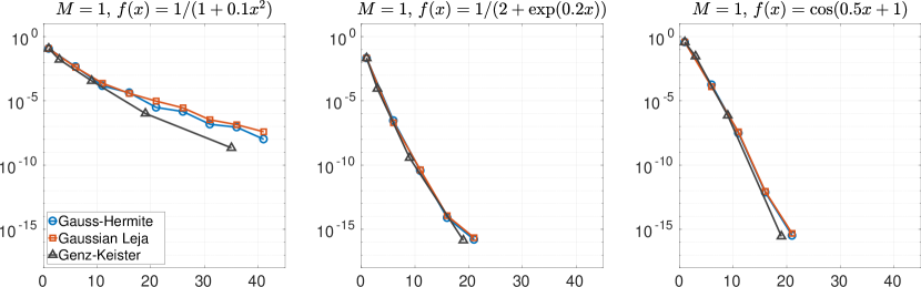
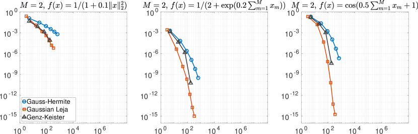
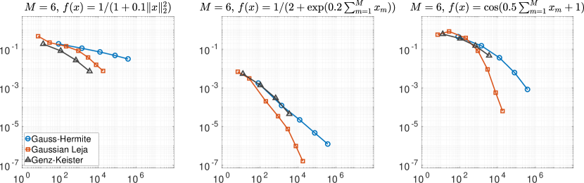
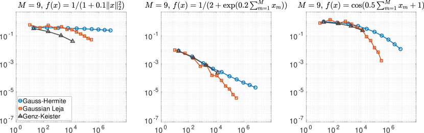
Figure 4: $L^{2}_{\mu}$ error for univariate and multivariate interpolation. The results for the univariate test were produced with $K=30$ repetitions, each with $P=100$ samples. The results for the multivariate test were produced with $K=50$ repetitions, each with $P=500$ samples.

4 Numerical Results

We now perform numerical tests solving the elliptic PDE introduced in Section 2, with the aim of extending the numerical evidence obtained in ErnstEtAl2018 . In that paper, we assessed:

• the sharpness of the predicted rate for the a-priori sparse grid construction (both with respect to the number of multi-indices in the set and the number of points in the sparse grids);

• the comparison in performance of the a-priori and the classical dimension-adaptive a-posteriori sparse grid constructions;

limiting ourselves to Gauss–Hermite collocation points, which are covered by our theory. The findings indicated that our predicted rates are somewhat conservative. Specifically, the rates of convergence measured in numerical experiments were larger than the theoretical ones by a factor between 0.5 and 1, cf. (ErnstEtAl2018, , Table 1). This is due to some technical estimates applied in the proof of the convergence results which we were so far not able to improve. Concerning the second point, we observed in ErnstEtAl2018 that the a-priori construction is actually competitive with the a-posteriori adaptive variant, especially if one considers the extra PDE solves needed to explore the set of multi-indices.

We remark in particular that we observed convergence of the sparse grid approximations even in cases in which the theory predicted no convergence (albeit with a rather poor convergence rate, comparable to that attainable with Monte Carlo or Quasi Monte Carlo methods—see also NobileEtAl2016 ; tesei:MCCV for possible remedies).

In this contribution, our goal is the numerical investigation of additional questions that so far remain unanswered by existing theory, among these:

1. whether using Gaussian Leja or Genz–Keister nodes yields improvement over Gauss–Hermite nodes in our framework, see Section 4.1;

2. whether changing the random field representation from Karhunen-Loève (KL) to Lévy-Ciesielski (LC) expansion for the case $q=1$ (pure Brownian bridge) improves the efficiency of the numerical computations, see Section 4.2. As explained above, this is motivated by the fact that LC expansion of the random field allowed BachmayrEtAl2015 to prove convergence of the best-N-term approximation of the lognormal problem over Hermite polynomials.

The tests were performed using the Sparse Grids Matlab Kit. We briefly recall the basic approaches of the two heuristics employed for constructing the multi-index sets $\Lambda$. We refer to ErnstEtAl2018 for the full details of the two algorithms. The first is the classical dimension-adaptive algorithm introduced by Gerstner and Griebel in GerstnerGriebel2003 with some suitable modifications to make it work with non-nested quadrature rules and for quadrature/interpolation on unbounded domains. It is driven by a posteriori error indicators computed along the outer margin of the current multi-index set. The mechanism by which new random variables are activated in the multi-index set uses a “buffer” of fixed size containing variables whose error indicators have been computed but not yet selected. The second approach is an a-priori tailored choice of multi-index set $\Lambda$, which can be derived from the study of the decay of the spectral coefficients of the solution.

We thus consider the problem in Equation (1) with $f=1$. We set the pointwise standard deviation of $\log a$ to be $\sigma=3$; note that this constant does not appear explicitly in the expression for $\log a$ in Section 2, i.e., it has been absorbed in $\phi_{m}$. Figure 5 shows 30 realizations of the random field $a(\omega)$ for different values of $q$, obtained by truncating the Karhunen-Loève expansion of $a(\omega)$ at $M=1000$ random variables. Specifically, we consider a smoothed Brownian bridge as in Example 2, with $q=3,\,1.5,\,1$, cf. Equation (11); for these values of $q$ a truncation at 1000 random variables covers $100\%$, $99.99996\%$ and $99.93\%$ of the total variance of $\log a$, respectively. The plot shows how the realizations grow increasingly rough as $q$ decreases. Upon plotting the corresponding PDE solutions (not displayed for brevity) one would observe that, by contrast, solutions are much less rough, even in the case $q=1$.

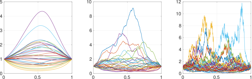
Figure 5: 30 realizations of the random field for different values of $q$. Left: $q=3$; center: $q=1.5$; right: $q=1$. Note the different scaling of the vertical axis.

4.1 Gauss–Hermite vs. Gaussian Leja vs. Genz–Keister nodes

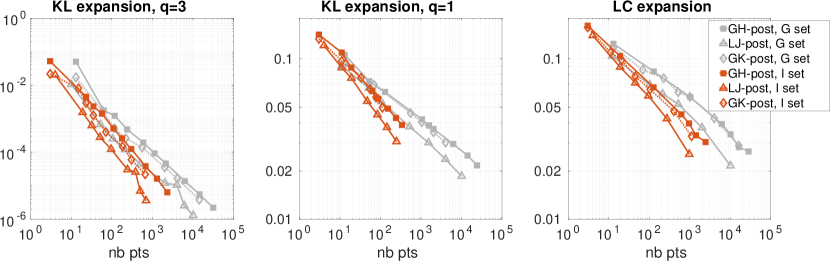
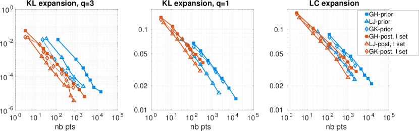
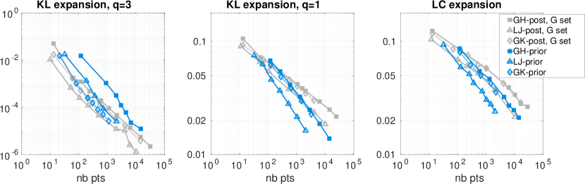
Figure 6: Comparison of performance for Gaussian Leja, Genz–Keister, and Gauss–Hermite points for different test cases and different sets of multi-indices. The plots report error versus number of points. To make the visual comparison easier we split the presentation into three parts. The top row shows the two different sets produced by the a-posteriori algorithm (a-posteriori-I-set-incremental and a-posteriori-G-set-incremental). The middle row compares a-priori and a-posteriori algorithms in terms of the optimal sets produced (a-priori-incremental and a-posteriori-I-set-incremental). The bottom row compares a-priori and a-posteriori algorithms in terms of bare computational cost (a-priori-incremental and a-posteriori-G-set-incremental).

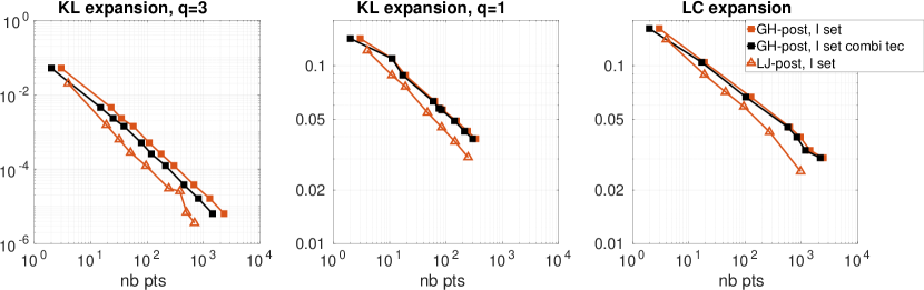
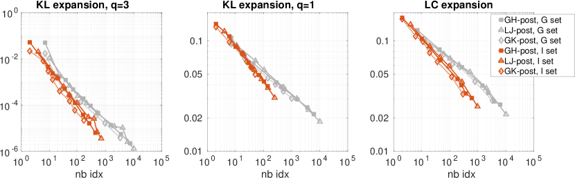
Figure 7: Top row: further analysis of influence of counting strategies in assessing the performance of Gaussian Leja, Genz–Keister, and Gauss–Hermite points. Middle and bottom rows: plot of error versus number of indices in the sparse grid set for different test cases. The plots in these two rows are grouped in the same way as in Figure 6.

We begin the analysis with the comparison of the performance of Gauss–Hermite, Gaussian Leja, and Genz–Keister points. To this end, we consider random fields of varying smoothness, we choose an expansion (KL/LC) for each random field considered, and we compute the sparse grid approximation of $u$ with the a-priori and a-posteriori dimension-adaptive sparse grid algorithm, with Gauss–Hermite, Gaussian Leja and Genz–Keister points (i.e., 6 runs per choice of random field and associated expansion). Specifically, we consider three different random field expansions, i.e., a KL expansion of the smoothed Brownian bridge with $q=3$, and a standard Brownian bridge ($q=1$) expanded with either KL or LC expansion, cf. again Examples 1 and 2. We compute the error in the full $L^{2}_{\mu}(\Gamma;H^{1}_{0}(D))$ norm again with a Monte Carlo sampling over 1000 samples of the random field, which has been verified to be sufficiently accurate for our purposes. These samples are generated considering a “reference truncation level” of the random field with 1000 random variables, which substantially exceeds the number of random variables active during the execution of the algorithms (which never involve more than a few hundred random variables). In the first set of results, we report the convergence of the error with respect to the number of points in the grid. The manner of counting of the points is a subtle issue and can be done in various ways. Here we consider the following different counting strategies:

“incremental”:

the number of points in the sparse grid $\Xi_{\Lambda}$ as defined in (17), i.e., the points required to compute the application of $U_{\Lambda}$ as given in (15),

“combitec”:

the number of points necessary for the combination technique representation of $U_{\Lambda}$ in (16); since $c(\mathbf{i};\Lambda)$ may be zero for some $\mathbf{i}\in\Lambda$, we can omit the corresponding $U_{\mathbf{i}}$ in (16) and consider the possibly smaller combitec sparse grid $\Xi^{\text{ct}}_{\Lambda}:=\bigcup_{\mathbf{i}\in\Lambda\colon c(\mathbf{i};\Lambda)\neq 0}\Xi^{(\mathbf{i})}$.

These strategies exhaust the counting strategies for the a-priori construction; note that these two counting schemes yield different values for non-nested points (such as Gauss–Hermite), while they are identical for nested points (such as Gaussian Leja and Genz–Keister). For the a-posteriori construction, one should also further decide whether to apply these counting strategies including or excluding the indices in the margin of the current set (“I-set” and “G-set” in the legend, respectively). Note that the “I-set” choice is more representative of the “optimal index-set” computed by the algorithm, while the “G-set” is more representative of the actual computational cost incurred when running the algorithm.

Results are reported in Figures 6 and 7. Throughout this section, we use the following abbreviations in the legend of the convergence plots: GH for Gauss–Hermite, LJ for Gaussian Leja, GK for Genz–Keister. Figure 6 compares the performance of the three choices of points for the three choices of random field expansions and the two sparse grid constructions mentioned earlier (a-posteriori/a-priori), in terms of $L^{2}_{\mu}$-error vs. number of collocation points. Different colors identify different combination of grid constructions and counting (light blue for a-priori-incremental; red for a-posteriori-I-set-incremental; gray for a-posteriori-G-set-incremental). The results for Gauss–Hermite points are indicated by solid lines with square filled markers, those for Gaussian Leja points by solid lines with empty triangle markers, and those for Genz–Keister by dashed lines with empty diamond markers.

The first and foremost observation to be made is that the Gaussian Leja performance is consistently better than Genz–Keister and Gauss–Hermite across algorithms (a-priori/a-posteriori) and test cases, while Gauss–Hermite and Genz–Keister performance is essentially identical, in agreement with what reported e.g. in NobileEtAl2016 ; Chen2016 . Only the Genz–Keister performance for the a-priori construction in the case $q=3$ is surprisingly good; we do not have an explanation for this, and leave it to future research. Secondly, we observe that the a-priori algorithm performs worse than the a-posteriori for $q=3$ (both considering the “G-set” and the “I-set” - left panel in the middle and bottom rows), while for the case $q=1$ it performs worse than the a-posteriori “I-set” but better than the a-posteriori “G-set” (regardless of type of expansion - mid and right panels in the central and bottom rows). This means that while there are better choices for the index set than a-priori one (e.g., the a-posteriori “I-set”), these might be hard to derive, so that in practice it might be convenient to use the a-priori algorithm. This is in agreement with the findings reported in ErnstEtAl2018 and not surprising, given that in the case $q=1$ features a larger number of random variables and therefore is harder to be handled by the a-posteriori algorithm.

In Figure 7 we analyze in more detail the relatively poor performance of Gauss–Hermite points. In the top row we want to investigate whether the “incremental”/“combitec” counting (which we recall produces different results only for Gauss–Hermite points) explains at least partially the gap between the Gauss–Hermite and the Gaussian Leja results in Figure 6. To this end, we focus on the a-posteriori “I-set”. For such grid and counting, we report the convergence curves from Figure 6 for both the Gauss–Hermite and the Gaussian Leja collocation points and add in black with filled markers the “combitec” counting, which is more favorable to Gauss–Hermite points. The plots show, however, that the counting method accounts for only a small fraction of the gap.

In the middle and bottom rows instead we investigate whether the set of multi-indices chosen by the algorithm also has an influence—in other words, could it be that because of the family of points, the algorithms are “tricked” into exploring less effective index sets? To this end, we redo Figure 6 by showing the convergence with respect to the number of multi-indices in the set $\Lambda$, instead of with respect to the number of points. The plots show that in this setting, there is essentially no difference in performance between Gauss–Hermite, Gaussian Leja and Genz–Keister points (again, excluding the case of Genz–Keister points for a-priori construction in the case $q=3)$, which means that the sets obtained by the a-priori/a-posteriori algorithm, while different, are “equally good” in approximating the solution. Thus, the consistent difference between Gaussian Leja, Genz–Keister and Gauss–Hermite nodes is really due to the nestedness of the former two choices. Between the two choices of nested points, the Gaussian Leja points are more granular and easier to compute up to an arbitrary number: in conclusion, they appear to be a more suitable choice of collocation points for the lognormal problem in terms of accuracy versus number of points.

4.2 KL vs. LC Expansion

The second set of tests aims at assessing whether expanding the random field over the wavelet basis (LC expansion) brings any practical advantage in convergence of the sparse grid algorithm over using the standard KL expansion. Since from the previous discussion we know that Gaussian Leja nodes are more effective than Gauss–Hermite and Genz–Keister points, we only consider Gaussian Leja points in this section.

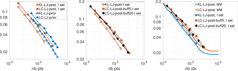
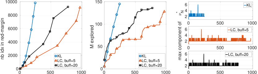
Figure 8: Comparison of performance for LC and KL expansions.

Figure 9: Evolution of the multi-index set $\Lambda$ for LC and KL expansions along iterations of the dimension-adaptive algorithm.

Results are reported in Figure 9. In the left plot, we compare the convergence of the error versus number of points for the a-priori and a-posteriori “I-set” for LC and KL expansion; we employ the same color-coding as in Figure 6 (blue for prior construction, red for the “I-set” of the a-posteriori construction), using filled markers for LC results and empty markers for KL results. The lines with filled markers are always significantly above the lines with empty markers, i.e., the convergence of the sparse grid adaptive algorithm is significantly faster for the KL expansion than for the LC expansion. This can easily be explained by the implicit ordering introduced by the KL expansion in the importance of the random variables: because the modes of the KL are ordered in descending order according to the percentage of variance of the random field they represent, they are already ordered in a suitable way for the adaptive algorithm, which from the very start can explore informative directions of variance (although the KL expansion is optimized for the representation of the input rather than for the output). The LC expansion instead uses a-priori choices of the expansion basis functions and in particular batches (of increasing cardinality) of those basis functions are equally important (i.e., the wavelets at the same refinement level). On the other hand, the adaptive algorithm explores random variables in the expansion order, which means that sometimes the algorithm has to include “unnecessary” modes of the LC expansion before finding those that really matter.

Of course, a careful implementation of the adaptive algorithm can, to a certain extent, mitigate this issue. In particular, increasing the size of the buffer of random variables (cf. the description at the beginning of Section 4) improves the performance of the adaptive algorithm. The default number of inactive random variables is 5—the convergence lines in the left plot are obtained in this way. In the middle plot we confirm that, as expected, increasing the buffer from 5 to 20 random variables improves the performance of the sparse grid approximation when applied to the LC case (black line with filled markers instead of red line with filled markers). Note, however, that a significant gap remains between the convergence of the sparse grid approximation for the LC expansion with a buffer of 20 random variables and the convergence of the sparse grid for the KL expansion. This means that not only does the buffer play a role, but the KL expansion is overall a more convenient basis to work with.

This aspect is further elaborated in the right plot of Figure 9. Here we show the convergence of the sparse grid approximation for KL (5-variable buffer) and LC (either 5-variable or 20-variable buffer) against the number of indices in the sparse grids (dashed lines with markers), and compare this convergence against an estimate of the corresponding best-N-term (bNt) expansion of the solution in Hermite polynomials (full lines without markers); different colors identify different expansions. Of course, the convergence of the bNt expansion also depends on the LC/KL basis, therefore we show two bNt convergence curves. The bNt was computed by converting the sparse grid into the equivalent Hermite expansion (see feal:compgeo ; lever.eal:inversion for details) and then rearranging the Hermite coefficients in order of decreasing magnitude. The plot shows that the sparse grid approximation of the solution by KL expansion is quite close to the bNt convergence (blue lines), which means that there is not much room for “compressibility” in the sparse grid approximation. Conversely, the 5-variable-buffer sparse grid approximation of the problem with LC expansion is somehow far from the bNt (red lines) and only the 20-variable-buffer (black dashed line) gets reasonably close: this means that the 5-variable-buffer is “forced” to add to the approximation “useless” indices merely because the ordering of the variables in the LC expansion is not optimal and the buffer is not large enough.

Finally, we report in Figure 9 some performance indicators for the construction of the index set for the KL and LC cases, which offer further insight towards explaining the superior KL performance. The figure on the left shows the growth of the size of the outer margin of the dimension-adaptive algorithm at each iteration, where we recall that one iteration is defined as the process of selecting one index from the outer margin and evaluating the error indicator for all its forward neighbors; this in particular means that the number of PDE solves per iteration is not fixed. All three algorithms (KL, 5-variable-buffer LC and 20-variable-buffer LC) stop after 10,000 PDE solves. KL displays the fastest growth in the outer margin size, followed by LC20 and then LC5, which is perhaps counter-intuitive; on the other hand, the more indices are considered, the more likely it is to find ones “effective” in reducing the approximation error. The figure in the center shows the growth in the number of explored dimensions: again, KL has the quickest and steadiest growth, which means that the algorithm favors adding new variables over exploring those already active. This might be again counter-intuitive, but there is no contradiction between this observation and the superior performance of KL: the point here is actually precisely the fact that the LC random variables are not conveniently sorted, so the algorithm is obliged to explore those already available rather than adding new ones; this is especially visible for the LC5 case, which displays a significant plateau in the growth in the number of variables in the middle of the algorithm execution. The three plots on the right finally show the largest component of multi-index $\mathbf{\nu}_{N}^{*}$ that has been selected from the reduced margin at iteration $N$ for the three algorithms (from the top: KL, LC5, LC20): a large maximum component means that the algorithm has favored exploring variables already activated, while if the maximum component is equal to 2 the algorithm has activated a new random variable (indices start from 1 in the Sparse Grids Matlab Kit). Most of the values in these plots are between 2 and 3, which again shows that the algorithms favor adding new variables rather than exploring those already available. Finally, we mention (plot omitted for brevity) that despite the relatively large number of random variables activated, each tensor grid in the sparse grid construction is at most 4-dimensional, which means that interactions between five or more of the random variables appearing in the KL or LC expansion, respectively, are considered negligible by the algorithm.

5 Conclusions

In this contribution we have investigated some practical choices related to the numerical approximation of random elliptic PDEs with lognormal diffusion coefficients by sparse grid collocation methods. More specifically, we discussed two issues, namely a) whether it pays off from a computational point of view to replace the classical Karhunen–Loève expansion of the log-diffusion field with the Lévy–Ciesielski expansion, as advocated in [2] for theoretical purposes and b) what type of univariate interpolation node sequence should be used in the sparse grid construction, choosing among Gauss–-Hermite, Gaussian Leja and Genz–-Keister points. Following a brief digression into the issue of convergence of interpolation and quadrature of univariate and multivariate functions based on these three classes of nodes, we compared the performance of sparse grid collocation for the approximate solution of the lognormal random PDEs in a number of different cases. The computational experiments suggest that Gaussian Leja collocation points, due to their approximation properties, granularity and nestedness, are the superior choice for the sparse grid approximation of the random PDE under consideration, and that the Karhunen–Loève expansion offers a computationally more effective parametrization of the input random field than the Lévy–Ciesielski expansion.

Appendix

We show that the Karhunen–Loève expansion of the Brownian bridge discussed in Example 1 does not satisfy the conditions of Theorem 2.1 for $p>0$. To this end, we first state

Proposition 3

Let $(b_{m})_{m\in\mathbb{N}}$ be a monotonely decreasing sequence of real numbers with $\lim_{m\to\infty}b_{m}=0$. Then for any $\theta\in[0,2\pi]$ we have

$$\sum_{m\geq 1}b_{m}\sin(m\theta)<\infty.$$

Proof

Dirichlet’s test for the convergence of series implies the statement if there exists a constant $K<\infty$ such that

$$\left|\sum_{m=1}^{M}\sin(m\theta)\right|\leq K\qquad\forall M\in\mathbb{N}.$$

Now, Lagrange’s trigonometric identity tells us that

$$\sum_{m=1}^{M}\sin(m\theta)=\frac{1}{2}\cot(0.5\theta)-\frac{\cos\left((M+0.5)\theta\right)}{2\sin(0.5\theta)},\qquad\theta\in(0,2\pi).$$

Hence, since $\sin(m0)=\sin(m2\pi)=0$ the statement follows easily.

Proposition 4

Given the Karhunen–Loève expansion of the Brownian bridge as in (9), the function

$$k_{\bm{\tau}}(x):=\sum_{m=1}^{\infty}\tau_{m}\frac{\sqrt{2}}{\pi m}\sin(m\pi x),\qquad x\in D=[0,1],$$

is pointwise well-defined for $\tau_{m}=m^{1/q}$ with $q>1$ in which case $(\tau_{m}^{-1})_{m\in\mathbb{N}}\in\ell^{p}(\mathbb{N})$ for any $p>q>1$. However, assuming that $k_{\bm{\tau}}\colon[0,1]\to\mathbb{R}$ is well-defined for a sequence $\bm{\tau}=(\tau_{m})_{m\in\mathbb{N}}$ with $(\tau^{-1}_{m})_{m\in\mathbb{N}}\in\ell^{p}(\mathbb{N})$ for a $p\leq 2$, then $k_{\bm{\tau}}\notin L^{\infty}(D)$.

Proof

The first statement follows by Proposition 3 and $\frac{\sqrt{2}}{\pi m}\tau_{m}=Cm^{1/q-1}\to 0$ as $m\to\infty$. The second statement follows by contracdiction. Assume that $k_{\bm{\tau}}\in L^{\infty}(D)$, then also $k_{\bm{\tau}}\in L^{2}(D)$ and via $\|k_{\bm{\tau}}\|_{L^{2}(D)}=\frac{1}{\pi^{2}}\sum_{m=1}^{\infty}\frac{\tau^{2}_{m}}{m^{2}}$ we have that $\tau^{2}_{m}\leq cm$ for a $c\geq 0$—otherwise $\|k_{\bm{\tau}}\|_{L^{2}(D)}=+\infty$. Thus, $\tau_{m}^{-p}\geq c^{-p/2}m^{-p/2}$ and since $\sum_{m\geq 1}m^{-p/2}<+\infty$ if and only if $p>2$, we end up with $(\tau_{m}^{-1})_{m\in\mathbb{N}}\notin\ell^{2}(\mathbb{N})$.

For values $p>2$ we provide the following numerical evidence: we choose $\tau_{m}=m^{1/p}$, i.e., $(\tau_{m}^{-1})_{m\in\mathbb{N}}\in\ell^{p+\epsilon}(\mathbb{N})$, $\epsilon>0$, and compute the values of the function $\kappa_{\bm{\tau}}(x)$ as given in Proposition 4 in a neighborhood of $x=0$ numerically. The reason we are interested in small values of $x$ is the fact that $\kappa_{\bm{\tau}}(x)$, $x\neq 0$, can be bounded by $\frac{1}{2}\cot(0.5\pi x)+\frac{1}{2\sin(0.5\pi x)}$ by means of Proposition 3. Thus, we expect a blow-up for small values of $x$. Indeed, we observe numerically that $\kappa_{\bm{\tau}}(x)$ for $\tau_{m}=m^{1/p}$ behaves like $x^{-1/p}$ for small values of $x>0$, see Figure 10. This implies that $\kappa_{\bm{\tau}}$ is unbounded in a neighborhood of $x=0$ for any of the above choices of $\tau_{m}$ and, therefore, does not satisfy the conditions of Theorem 2.1.

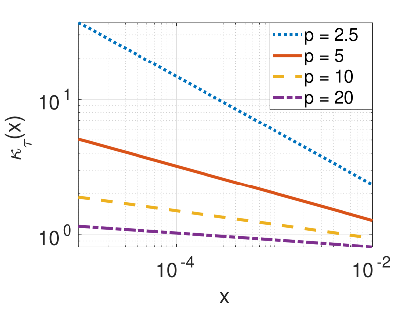
a

Figure 10: Growth of $\kappa_{\bm{\tau}}(x)$ as given in Proposition 4 for decaying $x\to 0+$ and choices $\tau_{m}=m^{1/p}$ with various values of $p$—the observed growth matches $x^{-1/p}$.

References

- (1) I. Babuška, F. Nobile, and R. Tempone. A stochastic collocation method for elliptic partial differential equations with random input data. SIAM Review, 52(2):317–355, June 2010.
- (2) M. Bachmayr, A. Cohen, R. DeVore, and G. Migliorati. Sparse polynomial approximation of parametric elliptic PDEs. part II: lognormal coefficients. ESAIM Math. Model. Numer. Anal., 51(1):321–339, 2016.
- (3) M. Bachmayr, A. Cohen, and G. Migliorati. Representations of Gaussian random fields and approximation of elliptic PDEs with lognormal coefficients. J. Fourier Anal. Appl., 18:621–649, 2018.
- (4) J. Baglama, D. Calvetti, and L. Reichel. Fast Leja points. Electronic Transactions on Numerical Analysis, 7:124–140, 1998.
- (5) V. Barthelmann, E. Novak, and K. Ritter. High dimensional polynomial interpolation on sparse grids. Advances in Computational Mathematics, 12:273–288, 2000.
- (6) A. Benassi, S. Jaffard, and R. D. Elliptic gaussian random processes. Revista Mathemática Iberoamericana, 13:19–90, 1997.
- (7) R. Bhattacharya and E. C. Waymire. A Basic Course in Probability Theory. Springer, Cham, 2nd edition, 2016.
- (8) B. Bohn, M. Griebel, and J. Oettershagen. Optimally rotated coordinate systems for adaptive least-squares regression on sparse grids. arXiv:1604.08466, 2018.
- (9) J. Charrier. Strong and weak error estimates for elliptic partial differential equations with random coefficients. SIAM Journal on Numerical Analysis, 50(1):216–246, 2012.
- (10) Chen, P. Sparse quadrature for high-dimensional integration with Gaussian measure. ESAIM: M2AN, 52(2):631–657, 2018.
- (11) Z. Ciesielski. Hölder condition for realization of gaussian processes. Trans. Amer. Math. Soc., 99:403–464, 1961.
- (12) F. E. Elliot, D. J. Horntrop, and A. J. Majda. A Fourier–wavelet Monte Carlo method for fractal random fields. Journal of Computational Physics, 132:384–408, 1994.
- (13) F. E. Elliot and A. J. Majda. A wavelet Monte Carlo method for turbulent diffusion with many spatial scales. Journal of Computational Physics, 113:82–111, 1994.
- (14) O. Ernst, B. Sprungk, and L. Tamellini. Convergence of sparse collocation for functions of countably many Gaussian random variables (with application to elliptic PDEs). SIAM J. Numer. Anal., 56(2):877–905, 2018.
- (15) I.-G. Farcas, J. Latz, E. Ullmann, T. Neckel, and H.-J. Bungartz. Multilevel adaptive sparse Leja approximations for Bayesian inverse problems. arXiv:1904.12204, 2019.
- (16) L. Formaggia, A. Guadagnini, I. Imperiali, V. Lever, G. Porta, M. Riva, A. Scotti, and L. Tamellini. Global sensitivity analysis through polynomial chaos expansion of a basin-scale geochemical compaction model. Computational Geosciences, 17(1):25–42, 2013.
- (17) R. A. Freeze. A stochastic-conceptual analysis of one-dimensional groundwater flow in nonuniform homogeneous media. Water Resources Research, 11(5):725–741, 1975.
- (18) J. Galvis and M. Sarkis. Approximating infinity-dimensional stochastic Darcy’s equations without uniform ellipticity. SIAM J. Numer. Anal., 47(5):3624–3651, 2009.
- (19) A. Genz and B. D. Keister. Fully symmetric interpolatory rules for multiple integrals over infinite regions with Gaussian weight. Journal of Computational and Applied Mathematics, 71(2):299–309, 1996.
- (20) T. Gerstner and M. Griebel. Dimension-adaptive tensor-product quadrature. Computing, 71(1):65–87, 2003.
- (21) R. Ghanem and P. Spanos. Stochastic Finite Elements: A Spectral Approach. Springer-Verlag, New York, 1991.
- (22) D. Gilbarg and N. S. Trudinger. Elliptic Partial Differential Equations of Second Order. Springer-Verlag, Berlin Heidelberg, 2001.
- (23) C. J. Gittelson. Stochastic Galerkin discretization of the log-normal isotropic diffusion problem. Math. Models Methods Appl. Sci., 20(2):237–263, 2010.
- (24) I. G. Graham, F. Y. Kuo, J. A. Nichols, R. Scheichl, C. Schwab, and I. H. Sloan. Quasi-Monte Carlo finite element methods for elliptic PDEs with lognormal random coefficients. Numer Math., 131:329–368, 2015.
- (25) H. Harbrecht, M. Peters, and M. Siebenmorgen. Multilevel accelerated quadrature for pdes with log-normally distributed diffusion coefficient. SIAM/ASA Journal on Uncertainty Quantification, 4(1):520–551, 2016.
- (26) F. Heiss and V. Winschel. Likelihood approximation by numerical integration on sparse grids. J. Econometrics, 144(1):62–80, 2008.
- (27) P. Jantsch, C. G. Webster, and G. Zhang. On the Lebesgue constant of weighted Leja points for Lagrange interpolation on unbounded domains. IMA Journal of Numerical Analysis, 39(2):1039–1057, 2019.
- (28) D. Loukrezis and H. De Gersem. Approximation and Uncertainty Quantification of Stochastic Systems with Arbitrary Input Distributions using Weighted Leja Interpolation. arXiv:1904.07709, 2019.
- (29) D. S. Lubinsky. A survey of weighted polynomial approximation with exponential weights. Surveys in Approximation Theory, 3:1–105, 2007.
- (30) H. Luschgy and G. Pagès. Expansions for Gaussian processes and Parseval frames. Electronic Journal of Probability, 14(42):1198–1221, 2009.
- (31) S. D. Marchi. On Leja sequences: some results and applications. Applied Mathematics and Computation, 152:621–647, 2004.
- (32) A. Mugler and H.-J. Starkloff. On the convergence of the stochastic Galerkin method for random elliptic partial differential equations. ESAIM: Mathematical Modelling and Numerical Analysis, 47(5):1237–1263, 2013.
- (33) A. Narayan and J. D. Jakeman. Adaptive Leja sparse grid constructions for stochastic collocation and high-dimensional approximation. SIAM Journal on Scientific Computing, 36(6):A2952–A2983, 2014.
- (34) S. Neuman, M. Riva, and A. Guadagnini. On the geostatistical characterization of hierarchical media. Water Resources Research, 44(2), 2008.
- (35) F. Nobile, L. Tamellini, F. Tesei, and R. Tempone. An adaptive sparse grid algorithm for elliptic PDEs with lognormal diffusion coefficient. In Sparse Grids and Applications – Stuttgart 2014. Springer-Verlag, 2016.
- (36) F. Nobile, R. Tempone, and C. Webster. An anisotropic sparse grid stochastic collocation method for partial differential equations with random input data. SIAM Journal on Numerical Analysis, 46(5):2411–2442, 2008.
- (37) F. Nobile, R. Tempone, and C. Webster. A sparse grid stochastic collocation method for partial differential equations with random input data. SIAM Journal on Numerical Analysis, 46(5):2309–2345, 2008.
- (38) F. Nobile and F. Tesei. A Multi Level Monte Carlo method with control variate for elliptic PDEs with log-normal coefficients. Stochastic Partial Differential Equations: Analysis and Computations, 3(3):398–444, 2015.
- (39) I. Papaioannou, M. Ehre, and D. Straub. PLS-based adaptation for efficient PCE representation in high dimensions. Journal of Computational Physics, 387:186 – 204, 2019.
- (40) G. Porta, L. Tamellini, V. Lever, and M. Riva. Inverse modeling of geochemical and mechanical compaction in sedimentary basins through polynomial chaos expansion. Water Resources Research, 50(12):9414–9431, 2014.
- (41) E. B. Saff and V. Totik. Logarithmic Potentials with External Fields, volume 316 of Grundlehren der mathematischen Wissenschaften. Springer, 1997.
- (42) C. Schwab and C. Gittelson. Sparse tensor discretizations of high-dimensional parametric and stochastic PDEs. Acta Numerica, 20:291–467, 2011.
- (43) B. Sprungk. Numerical Methods for Bayesian Inference in Hilbert Spaces. PhD thesis, TU Chemnitz, 2017.
- (44) L. Tamellini. Polynomial Approximation of PDEs with Stochastic Coefficients. PhD thesis, Politecnico di Milano, 2012.
- (45) R. Taylor and V. Totik. Lebesgue constants for Leja points. IMA Journal of Numerical Analysis, 30:462–486, 2010.
- (46) R. Tipireddy and R. Ghanem. Basis adaptation in homogeneous chaos spaces. Journal of Computational Physics, 259:304 – 317, 2014.
- (47) L. M. M. van den Bos, B. Sanderse, W. A. A. M. Bierbooms, and G. J. W. van Bussel. Bayesian model calibration with interpolating polynomials based on adaptively weighted Leja nodes. arXiv:1802.02035, 2018.
- (48) D. Xiu and J. Hesthaven. High-order collocation methods differential equations with random inputs. SIAM Journal on Scientific Computing, 37(3):1118–1139, 2005.