Universal Boosting Variational Inference

Abstract

Boosting variational inference (BVI) approximates an intractable probability density by iteratively building up a mixture of simple component distributions one at a time, using techniques from sparse convex optimization to provide both computational scalability and approximation error guarantees. But the guarantees have strong conditions that do not often hold in practice, resulting in degenerate component optimization problems; and we show that the ad-hoc regularization used to prevent degeneracy in practice can cause BVI to fail in unintuitive ways. We thus develop universal boosting variational inference (UBVI), a BVI scheme that exploits the simple geometry of probability densities under the Hellinger metric to prevent the degeneracy of other gradient-based BVI methods, avoid difficult joint optimizations of both component and weight, and simplify fully-corrective weight optimizations. We show that for any target density and any mixture component family, the output of UBVI converges to the best possible approximation in the mixture family, even when the mixture family is misspecified. We develop a scalable implementation based on exponential family mixture components and standard stochastic optimization techniques. Finally, we discuss statistical benefits of the Hellinger distance as a variational objective through bounds on posterior probability, moment, and importance sampling errors. Experiments on multiple datasets and models show that UBVI provides reliable, accurate posterior approximations.

1 Introduction

Bayesian statistical models provide a powerful framework for learning from data, with the ability to encode complex hierarchical dependence structures and prior domain expertise, as well as coherently capture uncertainty in latent parameters. The two predominant methods for Bayesian inference are Markov chain Monte Carlo (MCMC) [1, 2]—which obtains approximate posterior samples by simulating a Markov chain—and variational inference (VI) [3, 4]—which obtains an approximate distribution by minimizing some divergence to the posterior within a tractable family. The key strengths of MCMC are its generality and the ability to perform a computation-quality tradeoff: one can obtain a higher quality approximation by simulating the chain for a longer period [5, Theorem 4 & Fact 5]. However, the resulting Monte Carlo estimators have an unknown bias or random computation time [6], and statistical distances between the discrete sample posterior approximation and a diffuse true posterior are vacuous, ill-defined, or hard to bound without restrictive assumptions or a choice of kernel [7, 8, 9]. Designing correct MCMC schemes in the large-scale data setting is also a challenging task [10, 11, 12]. VI, on the other hand, is both computationally scalable and widely applicable due to advances from stochastic optimization and automatic differentiation [13, 14, 15, 16, 17]. However, the major disadvantage of the approach—and the fundamental reason that MCMC remains the preferred method in statistics—is that the variational family typically does not contain the posterior, fundamentally limiting the achievable approximation quality. And despite recent results in the asymptotic theory of variational methods [18, 19, 20, 21, 22], it is difficult to assess the effect of the chosen family on the approximation for finite data; a poor choice can result in severe underestimation of posterior uncertainty [23, Ch. 21].

Boosting variational inference (BVI) [24, 25, 26] is an exciting new approach that addresses this fundamental limitation by using a nonparametric mixture variational family. By adding and reweighting only a single mixture component at a time, the approximation may be iteratively refined, achieving the computation/quality tradeoff of MCMC and the scalability of VI. Theoretical guarantees on the convergence rate of Kullback-Leibler (KL) divergence [24, 27, 28] are much stronger than those available for standard Monte Carlo, which degrade as the number of estimands increases, enabling the practitioner to confidently reuse the same approximation for multiple tasks. However, the bounds require the KL divergence to be sufficiently smooth over the class of mixtures—an assumption that does not hold for many standard mixture families, e.g. Gaussians, resulting in a degenerate procedure in practice. To overcome this, an ad-hoc entropy regularization is typically added to each component optimization; but this regularization invalidates convergence guarantees, and—depending on the regularization weight—sometimes does not actually prevent degeneracy.

In this paper, we develop universal boosting variational inference (UBVI), a variational scheme based on the Hellinger distance rather than the KL divergence. The primary advantage of using the Hellinger distance is that it endows the space of probability densities with a particularly simple unit-spherical geometry in a Hilbert space. We exploit this geometry to prevent the degeneracy of other gradient-based BVI methods, avoid difficult joint optimizations of both component and weight, simplify fully-corrective weight optimizations, and provide a procedure in which the normalization constant of $f$ does not need to be known, a crucial property in most VI settings. It also leads to the universality of UBVI: we show that for any target density and any mixture component family, the output of UBVI converges to the best possible approximation in the mixture family, even when the mixture family is misspecified. We develop a scalable implementation based on exponential family mixture components and standard stochastic optimization techniques. Finally, we discuss other statistical benefits of the Hellinger distance as a variational objective through bounds on posterior probability, moment, and importance sampling errors. Experiments on multiple datasets and models show that UBVI provides reliable, accurate posterior approximations.

2 Background: variational inference and boosting

Variational inference, in its most general form, involves approximating a probability density $p$ by minimizing some divergence $\mathrm{D}\left(\cdot||\cdot\right)$ from $\xi$ to $p$ over densities $\xi$ in a family $\mathcal{Q}$,

$$q=\operatornamewithlimits{arg\,min}_{\xi\in\mathcal{Q}}\mathrm{D}\left(\xi||p\right).$$ (2)

Past work has almost exclusively involved parametric families $\mathcal{Q}$, such as mean-field exponential families [4], finite mixtures [29, 30, 31], normalizing flows [32], and neural nets [16]. The issue with these families is that typically $\min_{\xi\in\mathcal{Q}}\mathrm{D}\left(\xi||p\right)>0$—meaning the practitioner cannot achieve arbitrary approximation quality with more computational effort—and a priori, there is no way to tell how poor the best approximation is. To address this, boosting variational inference (BVI) [24, 25, 26] proposes the use of the nonparametric family of all finite mixtures of a component density family $\mathcal{C}$,

$$\mathcal{Q}=\operatorname{conv}{\mathcal{C}} :=\left\{\sum_{k=1}^{K}w_{k}\xi_{k}:K\in\mathbb{N},w\in\Delta^{K-1},\,\,\forall k\in\mathbb{N}\,\,\xi_{k}\in\mathcal{C}\right\}.$$ (3)

Given a judicious choice of $\mathcal{C}$, we have that $\inf_{\xi\in\mathcal{Q}}\mathrm{D}\left(\xi||p\right)=0$; in other words, we can approximate any continuous density $p$ with arbitrarily low divergence [33]. As optimizing directly over the nonparametric $\mathcal{Q}$ is intractable, BVI instead adds one component at a time to iteratively refine the approximation. There are two general formulations of BVI; Miller et al. [26] propose minimizing KL divergence over both the weight and component simultaneously,

$$\!\!\!q_{n} =\sum_{k=1}^{n}w_{nk}\xi_{k} \xi_{n+1},\omega =\operatornamewithlimits{arg\,min}_{\xi\in\mathcal{C},\rho\in[0,1]}\mathrm{D_{KL}}\left(\rho\xi+(1-\rho)q_{n}||p\right) w_{n+1}=\left[(1-\omega)w_{n}\,\,\omega\right]^{T}\!\!\!\!,$$ (4)

while Guo et al. and Wang [24, 25] argue that optimizing both simultaneously is too difficult, and use a gradient boosting [34] formulation instead,

$$\xi_{n+1} =\operatornamewithlimits{arg\,min}_{\xi\in\mathcal{C}}\left<\xi,\left.\nabla\mathrm{D_{KL}}\left(\cdot||p\right)\right|_{q_{n}}\right> w_{n+1} =\operatornamewithlimits{arg\,min}_{\omega=\left[(1-\rho)w_{n}\,\,\rho\right]^{T}\!\!\!\!,\,\,\rho\in[0,1]}\mathrm{D_{KL}}\left(\sum_{k=1}^{n+1}\omega_{k}\xi_{k}||p\right).$$ (5)

Both algorithms attain $\mathrm{D_{KL}}\left(q_{N}||p\right)=O(1/N)$— the former by appealing to results from convex functional analysis [35, Theorem II.1], and the latter by viewing BVI as functional Frank-Wolfe optimization [27, 36, 37]. This requires that $\mathrm{D_{KL}}\left(q||p\right)$ is strongly smooth or has bounded curvature over $q\in\mathcal{Q}$, for which it is sufficient that densities in $\mathcal{Q}$ are bounded away from 0, bounded above, and have compact support [27], or have a bounded parameter space [28]. However, these assumptions do not hold in practice for many simple (and common) cases, e.g., where $\mathcal{C}$ is the class of multivariate normal distributions. Indeed, gradient boosting-based BVI methods all require some ad-hoc entropy regularization in the component optimizations to avoid degeneracy [24, 25, 28]. In particular, given a sequence of regularization weights $r_{n}>0$, BVI solves the following component optimization [28]:

$$\xi_{n+1} =\operatornamewithlimits{arg\,min}_{\xi\in\mathcal{C}}\left<\xi,\log\frac{\xi^{r_{n+1}}q_{n}}{p}\right>.$$ (6)

This addition of regularization has an adverse effect on performance in practice as demonstrated in Fig. 1(b), and can lead to unintuitive behaviour and nonconvergence—even when $p\in\mathcal{Q}$ (Proposition 1) or when the distributions in $\mathcal{C}$ have lighter tails than $p$ (Proposition 2).

Proposition 1.

Suppose $\mathcal{C}$ is the set of univariate Gaussians with mean 0 parametrized by variance, let $p=\mathcal{N}(0,1)$, and let the initial approximation be $q_{1}=\mathcal{N}(0,\tau^{2})$. Then BVI in Eq. 6 with regularization $r_{2}>0$ returns a degenerate next component $\xi_{2}$ if $\tau^{2}\leq 1$, and iterates infinitely without improving the approximation if $\tau^{2}>1$ and $r_{2}>\tau^{2}-1$.

Proposition 2.

Suppose $\mathcal{C}$ is the set of univariate Gaussians with mean 0 parametrized by variance, and let $p=\mathrm{Cauchy}(0,1)$. Then BVI in Eq. 6 with regularization $r_{1}>0$ returns a degenerate first component $\xi_{1}$ if $r_{1}\geq 2$.

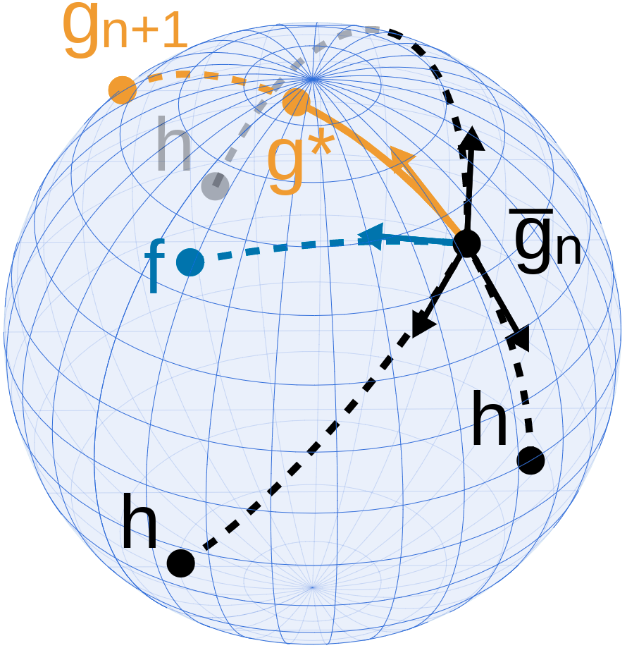
(a)

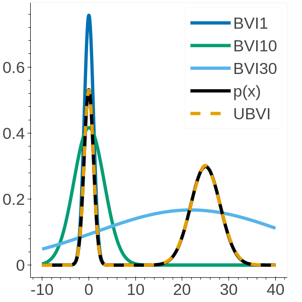
(b)

Figure 1: (1(a)): Greedy component selection, with target $f$, current iterate $\bar{g}_{n}$, candidate components $h$, optimal component $g_{n+1}$, the closest point $g^{\star}$ to $f$ on the $\bar{g}_{n}\to g_{n+1}$ geodesic, and arrows for initial geodesic directions. The quality of $g_{n+1}$ is determined by the distance from $f$ to $g^{\star}$, or equivalently, by the alignment of the initial directions $\bar{g}_{n}\to g_{n+1}$ and $\bar{g}_{n}\to f$. (1(b)): BVI can fail even when $p$ is in the mixture family. Here $p=\frac{1}{2}\mathcal{N}(0,1)+\frac{1}{2}\mathcal{N}(25,5)$, and UBVI finds the correct mixture in 2 iterations. BVI (with regularization weight in $\{1,10,30\}$) does not converge. For example, when the regularization weight is 1 the first component will have variance $<5$, and the second component optimization diverges since the target $\mathcal{N}(25,5)$ component has a heavier tail. Upon reweighting the second component is removed, and the approximation will never improve.

3 Universal boosting variational inference (UBVI)

3.1 Algorithm and convergence guarantee

To design a BVI procedure without the need for ad-hoc regularization, we use a variational objective based on the Hellinger distance, which for any probability space $(\mathcal{X},\Sigma,\mu)$ and densities $p,q$ is

$$\mathrm{D^{2}_{H}}\left(p,q\right) :=\frac{1}{2}\int\left(\mathchoice{{\hbox{$\displaystyle\sqrt{p(x)\,}$}\lower 0.4pt\hbox{\vrule height=7.5pt,depth=-6.00003pt}}}{{\hbox{$\textstyle\sqrt{p(x)\,}$}\lower 0.4pt\hbox{\vrule height=7.5pt,depth=-6.00003pt}}}{{\hbox{$\scriptstyle\sqrt{p(x)\,}$}\lower 0.4pt\hbox{\vrule height=5.25pt,depth=-4.20003pt}}}{{\hbox{$\scriptscriptstyle\sqrt{p(x)\,}$}\lower 0.4pt\hbox{\vrule height=3.75pt,depth=-3.00002pt}}}-\mathchoice{{\hbox{$\displaystyle\sqrt{q(x)\,}$}\lower 0.4pt\hbox{\vrule height=7.5pt,depth=-6.00003pt}}}{{\hbox{$\textstyle\sqrt{q(x)\,}$}\lower 0.4pt\hbox{\vrule height=7.5pt,depth=-6.00003pt}}}{{\hbox{$\scriptstyle\sqrt{q(x)\,}$}\lower 0.4pt\hbox{\vrule height=5.25pt,depth=-4.20003pt}}}{{\hbox{$\scriptscriptstyle\sqrt{q(x)\,}$}\lower 0.4pt\hbox{\vrule height=3.75pt,depth=-3.00002pt}}}\right)^{2}\mu(\mathrm{d}x).$$ (7)

Our general approach relies on two facts about the Hellinger distance. First, the metric $\mathrm{D_{H}}\left(\cdot,\cdot\right)$ endows the set of $\mu$-densities with a simple geometry corresponding to the nonnegative functions on the unit sphere in $L^{2}(\mu)$. In particular, if $f,g\in L^{2}(\mu)$ satisfy $\|f\|_{2}=\|g\|_{2}=1$, $f,g\geq 0$, then $p=f^{2}$ and $q=g^{2}$ are probability densities and

$$\mathrm{D^{2}_{H}}\left(p,q\right)=\frac{1}{2}\left\|f-g\right\|_{2}^{2}.$$ (8)

One can thus perform Hellinger distance boosting by iteratively finding components that minimize geodesic distance to $f$ on the unit sphere in $L^{2}(\mu)$. Like the Miller et al. approach [26], the boosting step directly minimizes a statistical distance, leading to a nondegenerate method; but like the Guo et al. and Wang approach [24, 25], this avoids the joint optimization of both component and weight; see Section 3.2 for details. Second, a conic combination $g=\sum_{i=0}^{N}\lambda_{i}g_{i}$, $\lambda_{i}\geq 0$, $\|g_{i}\|_{2}=1$, $g_{i}\geq 0$ in $L^{2}(\mu)$ satisfying $\|g\|_{2}=1$ corresponds to the mixture model density

$$q=g^{2} =\sum_{i,j=1}^{N}Z_{ij}\lambda_{i}\lambda_{j}\left(\frac{g_{i}g_{j}}{Z_{ij}}\right) Z_{ij}:=\left<g_{i},g_{j}\right>\geq 0.$$ (9)

Therefore, if we can find a conic combination satisfying $\|f-g\|_{2}\leq\mathchoice{{\hbox{$\displaystyle\sqrt{2\,}$}\lower 0.4pt\hbox{\vrule height=6.44444pt,depth=-5.15558pt}}}{{\hbox{$\textstyle\sqrt{2\,}$}\lower 0.4pt\hbox{\vrule height=6.44444pt,depth=-5.15558pt}}}{{\hbox{$\scriptstyle\sqrt{2\,}$}\lower 0.4pt\hbox{\vrule height=4.51111pt,depth=-3.6089pt}}}{{\hbox{$\scriptscriptstyle\sqrt{2\,}$}\lower 0.4pt\hbox{\vrule height=3.22221pt,depth=-2.57779pt}}}\epsilon$ for $p=f^{2}$, we can guarantee that the corresponding mixture density $q$ satisfies $\mathrm{D_{H}}\left(p,q\right)\leq\epsilon$. The mixture will be built from a family $\mathcal{H}\subset L^{2}(\mu)$ of component functions for which $\forall h\in\mathcal{H}$, $\|h\|_{2}=1$ and $h\geq 0$. We assume that the target function $f\in L^{2}(\mu)$, $\|f\|_{2}=1$, $f\geq 0$ is known up to proportionality. We also assume that $f$ is not orthogonal to $\operatorname{span}{\mathcal{H}}$ for expositional brevity, although the algorithms and theoretical results presented here apply equally well in this case. We make no other assumptions; in particular, we do not assume $f$ is in $\operatorname{cl}{\operatorname{span}{\mathcal{H}}}$.

Algorithm 1 The universal boosting variational inference (UBVI) algorithm.

1:procedure UBVI($p$, $\mathcal{H}$, $N$)

2:    $f\overset{\propto}{\leftarrow}\mathchoice{{\hbox{$\displaystyle\sqrt{p\,}$}\lower 0.4pt\hbox{\vrule height=3.87498pt,depth=-3.1pt}}}{{\hbox{$\textstyle\sqrt{p\,}$}\lower 0.4pt\hbox{\vrule height=3.87498pt,depth=-3.1pt}}}{{\hbox{$\scriptstyle\sqrt{p\,}$}\lower 0.4pt\hbox{\vrule height=2.7125pt,depth=-2.17001pt}}}{{\hbox{$\scriptscriptstyle\sqrt{p\,}$}\lower 0.4pt\hbox{\vrule height=1.93748pt,depth=-1.55pt}}}$

3:    $\bar{g}_{0}\leftarrow 0$

4:    for $n=1,\dots,N$ do

5:          $\triangleright$ Find the next component to add to the approximation using Eq. 15

6:         $g_{n}\leftarrow\operatornamewithlimits{arg\,max}_{h\in\mathcal{H}}\left<f-\left<f,\bar{g}_{n-1}\right>\bar{g}_{n-1},h\right>\scalebox{0.75}{\bigg{/}}\mathchoice{{\hbox{$\displaystyle\sqrt{1-\left<h,\bar{g}_{n-1}\right>^{2}\,}$}\lower 0.4pt\hbox{\vrule height=6.47586pt,depth=-5.18071pt}}}{{\hbox{$\textstyle\sqrt{1-\left<h,\bar{g}_{n-1}\right>^{2}\,}$}\lower 0.4pt\hbox{\vrule height=6.47586pt,depth=-5.18071pt}}}{{\hbox{$\scriptstyle\sqrt{1-\left<h,\bar{g}_{n-1}\right>^{2}\,}$}\lower 0.4pt\hbox{\vrule height=5.67776pt,depth=-4.54224pt}}}{{\hbox{$\scriptscriptstyle\sqrt{1-\left<h,\bar{g}_{n-1}\right>^{2}\,}$}\lower 0.4pt\hbox{\vrule height=5.67776pt,depth=-4.54224pt}}}$

7:          $\triangleright$ Compute pairwise normalizations using Eq. 9

8:         for $i=1,\dots,n$ do

9:             $Z_{n,i}=Z_{i,n}\leftarrow\left<g_{n},g_{i}\right>$

10:         end for

11:          $\triangleright$ Update weights using Eq. 17

12:         $d=\left(\left<f,g_{1}\right>,\dots,\left<f,g_{n}\right>\right)^{T}$

13:         $\beta=\operatornamewithlimits{arg\,min}_{b\in\mathbb{R}^{n},b\geq 0}b^{T}Z^{-1}b+2b^{T}Z^{-1}d$

14:         $(\lambda_{n,1},\dots,\lambda_{n,n})=\frac{Z^{-1}(\beta+d)}{\mathchoice{{\hbox{$\displaystyle\sqrt{(\beta+d)^{T}Z^{-1}(\beta+d)\,}$}\lower 0.4pt\hbox{\vrule height=5.93039pt,depth=-4.74434pt}}}{{\hbox{$\textstyle\sqrt{(\beta+d)^{T}Z^{-1}(\beta+d)\,}$}\lower 0.4pt\hbox{\vrule height=5.93039pt,depth=-4.74434pt}}}{{\hbox{$\scriptstyle\sqrt{(\beta+d)^{T}Z^{-1}(\beta+d)\,}$}\lower 0.4pt\hbox{\vrule height=4.16849pt,depth=-3.33481pt}}}{{\hbox{$\scriptscriptstyle\sqrt{(\beta+d)^{T}Z^{-1}(\beta+d)\,}$}\lower 0.4pt\hbox{\vrule height=3.22348pt,depth=-2.5788pt}}}}$

15:          $\triangleright$ Update boosting approximation

16:         $\bar{g}_{n}\leftarrow\sum_{i=1}^{n}\lambda_{ni}g_{i}$

17:    end for

18:    return $q=\bar{g}^{2}_{N}$

19:end procedure

The universal boosting variational inference (UBVI) procedure is shown in Algorithm 1. In each iteration, the algorithm finds a new mixture component from $\mathcal{H}$ (line 5; see Section 3.2 and Fig. 1(a)). Once the new component is found, the algorithm solves a convex quadratic optimization problem to update the weights (lines 9–11). The primary requirement to run Algorithm 1 is the ability to compute or estimate $\left<h,f\right>$ and $\left<h,h^{\prime}\right>$ for $h,h^{\prime}\in\mathcal{H}$. For this purpose we employ an exponential component family $\mathcal{H}$ such that $Z_{ij}$ is available in closed-form, and use samples from $h^{2}$ to obtain estimates of $\left<h,f\right>$; see Appendix A for further implementation details.

The major benefit of UBVI is that it comes with a computation/quality tradeoff akin to MCMC: for any target $p$ and component family $\mathcal{H}$, (1) there is a unique mixture $\hat{p}=\hat{f}^{2}$ minimizing $\mathrm{D_{H}}\left(\hat{p},p\right)$ over the closure of finite mixtures $\operatorname{cl}{\mathcal{Q}}$; and (2) the output $q$ of UBVI$(p,\mathcal{H},N)$ satisfies $\mathrm{D_{H}}\left(q,\hat{p}\right)=O(1/N)$ with a dimension-independent constant. No matter how coarse the family $\mathcal{H}$ is, the output of UBVI will converge to the best possible mixture approximation. Theorem 3 provides the precise result.

Theorem 3.

For any density $p$ there is a unique density $\hat{p}=\hat{f}^{2}$ satisfying $\hat{p}=\operatornamewithlimits{arg\,min}_{\xi\in\operatorname{cl}{\mathcal{Q}}}\mathrm{D_{H}}\left(\xi,p\right)$. If each component optimization Eq. 15 is solved with a relative suboptimality of at most $(1-\delta)$, then the variational mixture approximation $q$ returned by UBVI($p$, $\mathcal{H}$, $N$) satisfies

$$\mathrm{D_{H}}\left(\hat{p},q\right)^{2} \leq\frac{J_{1}}{1+\left(\frac{1-\delta}{\tau}\right)^{2}J_{1}(N-1)} J_{1} :=1-\left<\hat{f},g_{1}\right>^{2}\in[0,1) \tau :=\text{\lx@cref{creftype~refnum}{eq:tau}}<\infty.$$ (10)

The proof of Theorem 3 may be found in Section B.3, and consists of three primary steps. First, Lemma 9 guarantees the existence and uniqueness of the convergence target $\hat{f}$ under possible misspecification of the component family $\mathcal{H}$. Then the difficulty of approximating $\hat{f}$ with conic combinations of functions in $\mathcal{H}$ is captured by the basis pursuit denoising problem [38]

$$\tau:=\inf_{\begin{subarray}{c}h_{i}\in\operatorname{cone}\mathcal{H}\\ x\in[0,1)\end{subarray}}\quad (1-x)^{-1}\sum_{i=1}^{\infty}\|h_{i}\|_{2}\quad\text{s.t.}\quad\|\hat{f}-\sum_{i=1}^{\infty}h_{i}\|_{2}\leq x,\quad\forall i,\,h_{i}\geq 0.$$ (11)

Lemma 10 guarantees that $\tau$ is finite, and in particular $\tau\leq\frac{\mathchoice{{\hbox{$\displaystyle\sqrt{1-J_{1}\,}$}\lower 0.4pt\hbox{\vrule height=4.78333pt,depth=-3.82668pt}}}{{\hbox{$\textstyle\sqrt{1-J_{1}\,}$}\lower 0.4pt\hbox{\vrule height=4.78333pt,depth=-3.82668pt}}}{{\hbox{$\scriptstyle\sqrt{1-J_{1}\,}$}\lower 0.4pt\hbox{\vrule height=3.34833pt,depth=-2.67868pt}}}{{\hbox{$\scriptscriptstyle\sqrt{1-J_{1}\,}$}\lower 0.4pt\hbox{\vrule height=2.39166pt,depth=-1.91335pt}}}}{1-\mathchoice{{\hbox{$\displaystyle\sqrt{J_{1}\,}$}\lower 0.4pt\hbox{\vrule height=4.78333pt,depth=-3.82668pt}}}{{\hbox{$\textstyle\sqrt{J_{1}\,}$}\lower 0.4pt\hbox{\vrule height=4.78333pt,depth=-3.82668pt}}}{{\hbox{$\scriptstyle\sqrt{J_{1}\,}$}\lower 0.4pt\hbox{\vrule height=3.34833pt,depth=-2.67868pt}}}{{\hbox{$\scriptscriptstyle\sqrt{J_{1}\,}$}\lower 0.4pt\hbox{\vrule height=2.39166pt,depth=-1.91335pt}}}}$, which can be estimated in practice using Eq. 24. Finally, Lemma 11 develops an objective function recursion, which is then solved to yield Theorem 3. Although UBVI and Theorem 3 is reminiscent of past work on greedy approximation in a Hilbert space [34, 39, 40, 41, 42, 43, 44, 45, 46], it provides the crucial advantage that the greedy steps do not require knowledge of the normalization of $p$. UBVI is inspired by a previous greedy method [46], but provides guarantees with an arbitrary, potentially misspecified infinite dictionary in a Hilbert space, and uses quadratic optimization to perform weight updates. Note that both the theoretical and practical cost of UBVI is dominated by finding the next component (line 5), which is a nonconvex optimization problem. The other expensive step is inverting $Z$; however, incremental methods using block matrix inversion [47, p. 46] reduce the cost at iteration $n$ to $O(n^{2})$ and overall cost to $O(N^{3})$, which is not a concern for practical mixtures with $\ll 10^{3}$ components. The weight optimization (line 10) is a nonnegative least squares problem, which can be solved efficiently [48, Ch. 23].

3.2 Greedy boosting along density manifold geodesics

This section provides the technical derivation of UBVI (Algorithm 1) by expoiting the geometry of square-root densities under the Hellinger metric. Let the conic combination in $L^{2}(\mu)$ after initialization followed by $N-1$ steps of greedy construction be denoted

$$\bar{g}_{n}:=\sum_{i=1}^{n}\lambda_{ni}g_{i},\quad\|\bar{g}_{n}\|_{2}=1,$$ (12)

where $\lambda_{ni}\geq 0$ is the weight for component $i$ at step $n$, and $g_{i}$ is the component added at step $i$. To find the next component, we minimize the distance between $\bar{g}_{n+1}$ and $f$ over choices of $h\in\mathcal{H}$ and position $x\in[0,1]$ along the $\bar{g}_{n}\to h$ geodesic,

$$\bar{g}_{0}=0\qquad g_{n+1},x^{\star} =\operatornamewithlimits{arg\,min}_{h\in\mathcal{H},x\in[0,1]}\left\|f-\left(x\frac{h-\left<h,\bar{g}_{n}\right>\bar{g}_{n}}{\|h-\left<h,\bar{g}_{n}\right>\bar{g}_{n}\|_{2}}+\mathchoice{{\hbox{$\displaystyle\sqrt{1-x^{2}\,}$}\lower 0.4pt\hbox{\vrule height=6.44444pt,depth=-5.15558pt}}}{{\hbox{$\textstyle\sqrt{1-x^{2}\,}$}\lower 0.4pt\hbox{\vrule height=6.44444pt,depth=-5.15558pt}}}{{\hbox{$\scriptstyle\sqrt{1-x^{2}\,}$}\lower 0.4pt\hbox{\vrule height=4.51111pt,depth=-3.6089pt}}}{{\hbox{$\scriptscriptstyle\sqrt{1-x^{2}\,}$}\lower 0.4pt\hbox{\vrule height=3.44165pt,depth=-2.75334pt}}}\bar{g}_{n}\right)\right\|_{2}$$ (13)

$$=\operatornamewithlimits{arg\,max}_{h\in\mathcal{H},x\in[0,1]}x\left<f,\frac{h-\left<h,\bar{g}_{n}\right>\bar{g}_{n}}{\|h-\left<h,\bar{g}_{n}\right>\bar{g}_{n}\|_{2}}\right>+\mathchoice{{\hbox{$\displaystyle\sqrt{1-x^{2}\,}$}\lower 0.4pt\hbox{\vrule height=6.44444pt,depth=-5.15558pt}}}{{\hbox{$\textstyle\sqrt{1-x^{2}\,}$}\lower 0.4pt\hbox{\vrule height=6.44444pt,depth=-5.15558pt}}}{{\hbox{$\scriptstyle\sqrt{1-x^{2}\,}$}\lower 0.4pt\hbox{\vrule height=4.51111pt,depth=-3.6089pt}}}{{\hbox{$\scriptscriptstyle\sqrt{1-x^{2}\,}$}\lower 0.4pt\hbox{\vrule height=3.44165pt,depth=-2.75334pt}}}\left<f,\bar{g}_{n}\right>.$$ (14)

Noting that $h-\left<h,\bar{g}_{n}\right>\bar{g}_{n}$ is orthogonal to $\bar{g}_{n}$, the second term does not depend on $h$, and $x\geq 0$, we avoid optimizing the weight and component simultaneously and find that

$$g_{n+1} =\operatornamewithlimits{arg\,max}_{h\in\mathcal{H}}\left<\frac{f-\left<f,\bar{g}_{n}\right>\bar{g}_{n}}{\|f-\left<f,\bar{g}_{n}\right>\bar{g}_{n}\|_{2}},\frac{h-\left<h,\bar{g}_{n}\right>\bar{g}_{n}}{\|h-\left<h,\bar{g}_{n}\right>\bar{g}_{n}\|_{2}}\right>=\operatornamewithlimits{arg\,max}_{h\in\mathcal{H}}\frac{\left<f-\left<f,\bar{g}_{n}\right>\bar{g}_{n},h\right>}{\mathchoice{{\hbox{$\displaystyle\sqrt{1-\left<h,\bar{g}_{n}\right>^{2}\,}$}\lower 0.4pt\hbox{\vrule height=7.19542pt,depth=-5.75636pt}}}{{\hbox{$\textstyle\sqrt{1-\left<h,\bar{g}_{n}\right>^{2}\,}$}\lower 0.4pt\hbox{\vrule height=7.19542pt,depth=-5.75636pt}}}{{\hbox{$\scriptstyle\sqrt{1-\left<h,\bar{g}_{n}\right>^{2}\,}$}\lower 0.4pt\hbox{\vrule height=5.67776pt,depth=-4.54224pt}}}{{\hbox{$\scriptscriptstyle\sqrt{1-\left<h,\bar{g}_{n}\right>^{2}\,}$}\lower 0.4pt\hbox{\vrule height=5.67776pt,depth=-4.54224pt}}}}.$$ (15)

Intuitively, Eq. 15 attempts to maximize alignment of $g_{n+1}$ with the residual $f-\left<f,\bar{g}_{n}\right>\bar{g}_{n}$ (the numerator) resulting in a ring of possible solutions, and among these, Eq. 15 minimizes alignment with the current iterate $\bar{g}_{n}$ (the denominator). The first form in Eq. 15 provides an alternative intuition: $g_{n+1}$ achieves the maximal alignment of the initial geodesic directions $\bar{g}_{n}\to f$ and $\bar{g}_{n}\to h$ on the sphere. See Fig. 1(a) for a depiction. After selecting the next component $g_{n+1}$, one option to obtain $\bar{g}_{n+1}$ is to use the optimal weighting $x^{\star}$ from Eq. 13; in practice, however, it is typically the case that solving Eq. 15 is expensive enough that finding the optimal set of coefficients for $\{g_{1},\dots,g_{n+1}\}$ is worthwhile. This is accomplished by maximizing alignment with $f$ subject to a nonnegativity and unit-norm constraint:

$$(\lambda_{(n+1)1},\dots,\lambda_{(n+1)(n+1)})=\operatornamewithlimits{arg\,max}_{x\in\mathbb{R}^{n+1}}\quad \left<f,\sum_{i=1}^{n+1}x_{i}g_{i}\right>\quad\text{s.t.}\quad x\geq 0,\quad x^{T}Zx\leq 1,$$ (16)

where $Z\in\mathbb{R}^{N+1\times N+1}$ is the matrix with entries $Z_{ij}$ from Eq. 9. Since projection onto the feasible set of Eq. 16 may be difficult, the problem may instead be solved using the dual via

$$\begin{aligned} &(\lambda_{(n+1)1},\dots,\lambda_{(n+1)(n+1)})=\frac{Z^{-1}(\beta+d)}{\mathchoice{{\hbox{$\displaystyle\sqrt{(\beta+d)^{T}Z^{-1}(\beta+d)\,}$}\lower 0.4pt\hbox{\vrule height=9.41333pt,depth=-7.5307pt}}}{{\hbox{$\textstyle\sqrt{(\beta+d)^{T}Z^{-1}(\beta+d)\,}$}\lower 0.4pt\hbox{\vrule height=9.41333pt,depth=-7.5307pt}}}{{\hbox{$\scriptstyle\sqrt{(\beta+d)^{T}Z^{-1}(\beta+d)\,}$}\lower 0.4pt\hbox{\vrule height=6.61667pt,depth=-5.29337pt}}}{{\hbox{$\scriptscriptstyle\sqrt{(\beta+d)^{T}Z^{-1}(\beta+d)\,}$}\lower 0.4pt\hbox{\vrule height=5.11667pt,depth=-4.09335pt}}}}\\ &d=\left(\left<f,g_{1}\right>,\dots,\left<f,g_{n+1}\right>\right)^{T}\qquad\beta=\operatornamewithlimits{arg\,min}_{b\in\mathbb{R}^{n+1},b\geq 0}b^{T}Z^{-1}b+2b^{T}Z^{-1}d.\end{aligned}$$ (17)

Eq. 17 is a nonnegative linear least-squares problem—for which very efficient algorithms are available [48, Ch. 23]—in contrast to prior variational boosting methods, where a fully-corrective weight update is a general constrained convex optimization problem. Note that, crucially, none of the above steps rely on knowledge of the normalization constant of $f$.

4 Hellinger distance as a variational objective

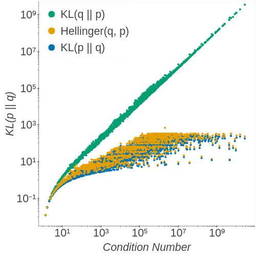
(a)

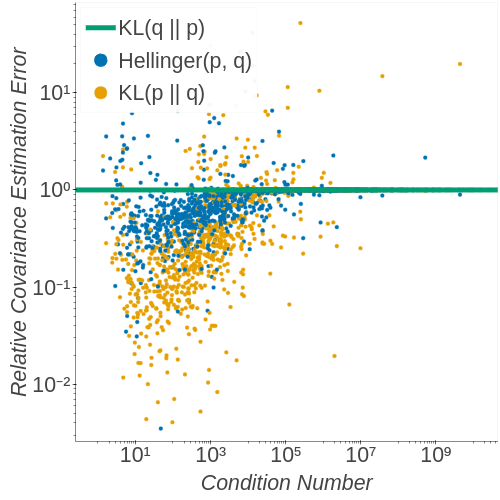
(b)

Figure 2: Forward KL divergence—which controls worst-case downstream importance sampling error—and importance-sampling-based covariance estimation error on a task of approximating $\mathcal{N}(0,A^{T}A)$, $A_{ij}\overset{\textrm{\tiny{i.i.d.}\@}}{\sim}\mathcal{N}(0,1)$ with $\mathcal{N}(0,\sigma^{2}I)$ by minimizing Hellinger, forward KL, and reverse KL, plotted as a function of condition number $\kappa(A^{T}A)$. Minimizing Hellinger distance provides significantly lower forward KL divergence and estimation error than minimizing reverse KL.

While the Hellinger distance has most frequently been applied in asymptotic analyses (e.g., [49]), it has seen recent use as a variational objective [50] and possesses a number of particularly useful properties that make it a natural fit for this purpose. First, $\mathrm{D_{H}}\left(\cdot,\cdot\right)$ applies to any arbitrary pair of densities, unlike $\mathrm{D_{KL}}\left(p||q\right)$, which requires that $p\ll q$. Minimizing $\mathrm{D_{H}}\left(\cdot,\cdot\right)$ also implicitly minimizes error in posterior probabilities and moments—two quantities of primary importance to practitioners—via its control on total variation and $\ell$-Wasserstein by Propositions 4 and 5. Note that the upper bound in Proposition 4 is typically tighter than that provided by the usual $\mathrm{D_{KL}}\left(q||p\right)$ variational objective via Pinsker’s inequality (and at the very least is always in $[0,1]$), and the bound in Proposition 5 shows that convergence in $\mathrm{D_{H}}\left(\cdot,\cdot\right)$ implies convergence in up to $\ell^{\text{th}}$ moments [51, Theorem 6.9] under relatively weak conditions.

Proposition 4 (e.g. [52, p. 61]).

The Hellinger distance bounds total variation via

$$\mathrm{D^{2}_{H}}\left(p,q\right) \leq\mathrm{D_{TV}}\left(p,q\right):=\frac{1}{2}\|p-q\|_{1}\leq\mathrm{D_{H}}\left(p,q\right)\mathchoice{{\hbox{$\displaystyle\sqrt{2-\mathrm{D^{2}_{H}}\left(p,q\right)\,}$}\lower 0.4pt\hbox{\vrule height=8.63776pt,depth=-6.91023pt}}}{{\hbox{$\textstyle\sqrt{2-\mathrm{D^{2}_{H}}\left(p,q\right)\,}$}\lower 0.4pt\hbox{\vrule height=8.63776pt,depth=-6.91023pt}}}{{\hbox{$\scriptstyle\sqrt{2-\mathrm{D^{2}_{H}}\left(p,q\right)\,}$}\lower 0.4pt\hbox{\vrule height=6.0722pt,depth=-4.85779pt}}}{{\hbox{$\scriptscriptstyle\sqrt{2-\mathrm{D^{2}_{H}}\left(p,q\right)\,}$}\lower 0.4pt\hbox{\vrule height=4.70554pt,depth=-3.76445pt}}}.$$ (18)

Proposition 5.

Suppose $\mathcal{X}$ is a Polish space with metric $d(\cdot,\cdot)$, $\ell\geq 1$, and $p,q$ are densities with respect to a common measure $\mu$. Then for any $x_{0}$,

$$W_{\ell}(p,q) \leq 2\mathrm{D_{H}}\left(p,q\right)^{\nicefrac{{1}}{{\ell}}}\left(\mathbb{E}\left[d(x_{0},X)^{2\ell}\right]+\mathbb{E}\left[d(x_{0},Y)^{2\ell}\right]\right)^{\nicefrac{{1}}{{2\ell}}},$$ (19)

where $Y\sim p(y)\mu(\mathrm{d}y)$ and $X\sim q(x)\mu(\mathrm{d}x)$. In particular, if densities $(q_{N})_{N\in\mathbb{N}}$ and $p$ have uniformly bounded $2\ell^{\text{th}}$ moments, $\mathrm{D_{H}}\left(p,q_{N}\right)\to 0\implies W_{\ell}(p,q_{N})\to 0$ as $N\to\infty$.

Once a variational approximation $q$ is obtained, it will typically be used to estimate expectations of some function of interest $\phi(x)\in L^{2}(\mu)$ via Monte Carlo. Unless $q$ is trusted entirely, this involves importance sampling—using $I_{n}(\phi)$ or $J_{n}(\phi)$ in Eq. 20 depending on whether the normalization of $p$ is known—to account for the error in $q$ compared with the target distribution $p$ [53],

$$I_{n}(\phi) :=\frac{1}{N}\sum_{n=1}^{N}\frac{p(X_{i})}{q(X_{i})}\phi(X_{i}) J_{n}(\phi) :=\frac{I_{n}(\phi)}{I_{n}(1)} X_{i} \overset{\textrm{\tiny{i.i.d.}\@}}{\sim}q(x)\mu(\mathrm{d}x).$$ (20)

Recent work has shown that the error of importance sampling is controlled by the intractable forward KL-divergence $\mathrm{D_{KL}}\left(p||q\right)$ [54]. This is where the Hellinger distance shines; Proposition 6 shows that it penalizes both positive and negative values of $\log p(x)/q(x)$ and thus provides moderate control on $\mathrm{D_{KL}}\left(p||q\right)$—unlike $\mathrm{D_{KL}}\left(q||p\right)$, which only penalizes negative values. See Fig. 2 for a demonstration of this effect on the classical correlated Gaussian example [23, Ch. 21]. While the takeaway from this setup is typically that minimizing $\mathrm{D_{KL}}\left(q||p\right)$ may cause severe underestimation of variance, a reasonable practitioner should attempt to use importance sampling to correct for this anyway. But Fig. 2 shows that minimizing $\mathrm{D_{KL}}\left(q||p\right)$ doesn’t minimize $\mathrm{D_{KL}}\left(p||q\right)$ well, leading to poor estimates from importance sampling. Even though minimizing $\mathrm{D_{H}}\left(p,q\right)$ also underestimates variance, it provides enough control on $\mathrm{D_{KL}}\left(p||q\right)$ so that importance sampling can correct the errors. Direct bounds on the error of importance sampling estimates are also provided in Proposition 7.

Proposition 6.

Define $R:=\log\frac{p(X)}{q(X)}$ where $X\sim p(x)\mu(\mathrm{d}x)$. Then

$$\mathrm{D_{H}}\left(p,q\right) \geq\frac{1}{2}\mathchoice{{\hbox{$\displaystyle\sqrt{\mathbb{E}\left[R^{2}\left(\frac{1+\mathds{1}\left[R\leq 0\right]R}{1+R}\right)^{2}\right]\,}$}\lower 0.4pt\hbox{\vrule height=13.83331pt,depth=-11.0667pt}}}{{\hbox{$\textstyle\sqrt{\mathbb{E}\left[R^{2}\left(\frac{1+\mathds{1}\left[R\leq 0\right]R}{1+R}\right)^{2}\right]\,}$}\lower 0.4pt\hbox{\vrule height=9.68332pt,depth=-7.74669pt}}}{{\hbox{$\scriptstyle\sqrt{\mathbb{E}\left[R^{2}\left(\frac{1+\mathds{1}\left[R\leq 0\right]R}{1+R}\right)^{2}\right]\,}$}\lower 0.4pt\hbox{\vrule height=6.91666pt,depth=-5.53336pt}}}{{\hbox{$\scriptscriptstyle\sqrt{\mathbb{E}\left[R^{2}\left(\frac{1+\mathds{1}\left[R\leq 0\right]R}{1+R}\right)^{2}\right]\,}$}\lower 0.4pt\hbox{\vrule height=6.91666pt,depth=-5.53336pt}}}\geq\frac{\mathrm{D_{KL}}\left(p||q\right)}{2\mathchoice{{\hbox{$\displaystyle\sqrt{1+\mathbb{E}\left[\mathds{1}\left[R>0\right](1+R)^{2}\right]\,}$}\lower 0.4pt\hbox{\vrule height=9.30444pt,depth=-7.44359pt}}}{{\hbox{$\textstyle\sqrt{1+\mathbb{E}\left[\mathds{1}\left[R>0\right](1+R)^{2}\right]\,}$}\lower 0.4pt\hbox{\vrule height=9.30444pt,depth=-7.44359pt}}}{{\hbox{$\scriptstyle\sqrt{1+\mathbb{E}\left[\mathds{1}\left[R>0\right](1+R)^{2}\right]\,}$}\lower 0.4pt\hbox{\vrule height=6.53888pt,depth=-5.23112pt}}}{{\hbox{$\scriptscriptstyle\sqrt{1+\mathbb{E}\left[\mathds{1}\left[R>0\right](1+R)^{2}\right]\,}$}\lower 0.4pt\hbox{\vrule height=5.03888pt,depth=-4.03113pt}}}}.$$ (21)

Proposition 7.

Define $\alpha:=\left(N^{-\nicefrac{{1}}{{4}}}+2\mathchoice{{\hbox{$\displaystyle\sqrt{\mathrm{D_{H}}\left(p,q\right)\,}$}\lower 0.4pt\hbox{\vrule height=7.5pt,depth=-6.00003pt}}}{{\hbox{$\textstyle\sqrt{\mathrm{D_{H}}\left(p,q\right)\,}$}\lower 0.4pt\hbox{\vrule height=7.5pt,depth=-6.00003pt}}}{{\hbox{$\scriptstyle\sqrt{\mathrm{D_{H}}\left(p,q\right)\,}$}\lower 0.4pt\hbox{\vrule height=5.25pt,depth=-4.20003pt}}}{{\hbox{$\scriptscriptstyle\sqrt{\mathrm{D_{H}}\left(p,q\right)\,}$}\lower 0.4pt\hbox{\vrule height=3.75pt,depth=-3.00002pt}}}\right)^{2}$. Then the importance sampling error with known normalization is bounded by

$$\mathbb{E}\left[\left|I_{n}(\phi)-I(\phi)\right|\right] \leq\|\mathchoice{{\hbox{$\displaystyle\sqrt{p\,}$}\lower 0.4pt\hbox{\vrule height=4.30554pt,depth=-3.44446pt}}}{{\hbox{$\textstyle\sqrt{p\,}$}\lower 0.4pt\hbox{\vrule height=4.30554pt,depth=-3.44446pt}}}{{\hbox{$\scriptstyle\sqrt{p\,}$}\lower 0.4pt\hbox{\vrule height=3.01389pt,depth=-2.41113pt}}}{{\hbox{$\scriptscriptstyle\sqrt{p\,}$}\lower 0.4pt\hbox{\vrule height=2.15277pt,depth=-1.72223pt}}}\phi\|_{2}\alpha,$$ (22)

and with unknown normalization by

$$\forall t>0\qquad\mathbb{P}(|J_{n}(\phi)-I(\phi)|>\|\mathchoice{{\hbox{$\displaystyle\sqrt{p\,}$}\lower 0.4pt\hbox{\vrule height=4.30554pt,depth=-3.44446pt}}}{{\hbox{$\textstyle\sqrt{p\,}$}\lower 0.4pt\hbox{\vrule height=4.30554pt,depth=-3.44446pt}}}{{\hbox{$\scriptstyle\sqrt{p\,}$}\lower 0.4pt\hbox{\vrule height=3.01389pt,depth=-2.41113pt}}}{{\hbox{$\scriptscriptstyle\sqrt{p\,}$}\lower 0.4pt\hbox{\vrule height=2.15277pt,depth=-1.72223pt}}}\phi\|_{2}t) \leq\left(1+4t^{-1}\mathchoice{{\hbox{$\displaystyle\sqrt{1+t\,}$}\lower 0.4pt\hbox{\vrule height=6.44444pt,depth=-5.15558pt}}}{{\hbox{$\textstyle\sqrt{1+t\,}$}\lower 0.4pt\hbox{\vrule height=6.44444pt,depth=-5.15558pt}}}{{\hbox{$\scriptstyle\sqrt{1+t\,}$}\lower 0.4pt\hbox{\vrule height=4.51111pt,depth=-3.6089pt}}}{{\hbox{$\scriptscriptstyle\sqrt{1+t\,}$}\lower 0.4pt\hbox{\vrule height=3.22221pt,depth=-2.57779pt}}}\right)\alpha.$$ (23)

Next, the Hellinger distance between densities $q,p$ can be estimated with high relative accuracy given samples from $q$, enabling the use of the above bounds in practice. This involves computing either $\widehat{\mathrm{D^{2}_{H}}\left(p,q\right)}$ or $\widetilde{\mathrm{D^{2}_{H}}\left(p,q\right)}$ below, depending on whether the normalization of $p$ is known. The expected error of both of these estimates relative to $\mathrm{D_{H}}\left(p,q\right)$ is bounded via Proposition 8.

$$\widehat{\mathrm{D^{2}_{H}}\left(p,q\right)} :=1\!-\!\frac{1}{N}\sum_{n=1}^{N}\mathchoice{{\hbox{$\displaystyle\sqrt{\frac{p(X_{n})}{q(X_{n})}\,}$}\lower 0.4pt\hbox{\vrule height=15.0pt,depth=-12.00005pt}}}{{\hbox{$\textstyle\sqrt{\frac{p(X_{n})}{q(X_{n})}\,}$}\lower 0.4pt\hbox{\vrule height=10.5pt,depth=-8.40004pt}}}{{\hbox{$\scriptstyle\sqrt{\frac{p(X_{n})}{q(X_{n})}\,}$}\lower 0.4pt\hbox{\vrule height=7.5pt,depth=-6.00003pt}}}{{\hbox{$\scriptscriptstyle\sqrt{\frac{p(X_{n})}{q(X_{n})}\,}$}\lower 0.4pt\hbox{\vrule height=7.5pt,depth=-6.00003pt}}}, \!\!\widetilde{\mathrm{D^{2}_{H}}\left(p,q\right)} :=1\!-\!\frac{\frac{1}{N}\sum_{n=1}^{N}\mathchoice{{\hbox{$\displaystyle\sqrt{\frac{p(X_{n})}{q(X_{n})}\,}$}\lower 0.4pt\hbox{\vrule height=15.0pt,depth=-12.00005pt}}}{{\hbox{$\textstyle\sqrt{\frac{p(X_{n})}{q(X_{n})}\,}$}\lower 0.4pt\hbox{\vrule height=10.5pt,depth=-8.40004pt}}}{{\hbox{$\scriptstyle\sqrt{\frac{p(X_{n})}{q(X_{n})}\,}$}\lower 0.4pt\hbox{\vrule height=7.5pt,depth=-6.00003pt}}}{{\hbox{$\scriptscriptstyle\sqrt{\frac{p(X_{n})}{q(X_{n})}\,}$}\lower 0.4pt\hbox{\vrule height=7.5pt,depth=-6.00003pt}}}}{\mathchoice{{\hbox{$\displaystyle\sqrt{\frac{1}{N}\sum_{n=1}^{N}\frac{p(X_{n})}{q(X_{n})}\,}$}\lower 0.4pt\hbox{\vrule height=15.0pt,depth=-12.00005pt}}}{{\hbox{$\textstyle\sqrt{\frac{1}{N}\sum_{n=1}^{N}\frac{p(X_{n})}{q(X_{n})}\,}$}\lower 0.4pt\hbox{\vrule height=10.5pt,depth=-8.40004pt}}}{{\hbox{$\scriptstyle\sqrt{\frac{1}{N}\sum_{n=1}^{N}\frac{p(X_{n})}{q(X_{n})}\,}$}\lower 0.4pt\hbox{\vrule height=7.5pt,depth=-6.00003pt}}}{{\hbox{$\scriptscriptstyle\sqrt{\frac{1}{N}\sum_{n=1}^{N}\frac{p(X_{n})}{q(X_{n})}\,}$}\lower 0.4pt\hbox{\vrule height=7.5pt,depth=-6.00003pt}}}}, \!\!X_{n} \overset{\textrm{\tiny{i.i.d.}\@}}{\sim}q(x)\mu(\mathrm{d}x).$$ (24)

Proposition 8.

The mean absolute difference between the Hellinger squared estimates is

$$\mathbb{E}\left[\left|\widehat{\mathrm{D^{2}_{H}}\left(p,q\right)}-\mathrm{D_{H}}\left(p,q\right)^{2}\right|\right] \leq\frac{\mathrm{D_{H}}\left(p,q\right)\mathchoice{{\hbox{$\displaystyle\sqrt{2-\mathrm{D_{H}}\left(p,q\right)^{2}\,}$}\lower 0.4pt\hbox{\vrule height=9.30444pt,depth=-7.44359pt}}}{{\hbox{$\textstyle\sqrt{2-\mathrm{D_{H}}\left(p,q\right)^{2}\,}$}\lower 0.4pt\hbox{\vrule height=9.30444pt,depth=-7.44359pt}}}{{\hbox{$\scriptstyle\sqrt{2-\mathrm{D_{H}}\left(p,q\right)^{2}\,}$}\lower 0.4pt\hbox{\vrule height=6.53888pt,depth=-5.23112pt}}}{{\hbox{$\scriptscriptstyle\sqrt{2-\mathrm{D_{H}}\left(p,q\right)^{2}\,}$}\lower 0.4pt\hbox{\vrule height=5.03888pt,depth=-4.03113pt}}}}{\mathchoice{{\hbox{$\displaystyle\sqrt{N\,}$}\lower 0.4pt\hbox{\vrule height=6.83331pt,depth=-5.46667pt}}}{{\hbox{$\textstyle\sqrt{N\,}$}\lower 0.4pt\hbox{\vrule height=6.83331pt,depth=-5.46667pt}}}{{\hbox{$\scriptstyle\sqrt{N\,}$}\lower 0.4pt\hbox{\vrule height=4.78333pt,depth=-3.82668pt}}}{{\hbox{$\scriptscriptstyle\sqrt{N\,}$}\lower 0.4pt\hbox{\vrule height=3.41666pt,depth=-2.73334pt}}}}$$ (25)

$$\mathbb{E}\left[\left|\widetilde{\mathrm{D^{2}_{H}}\left(p,q\right)}-\mathrm{D_{H}}\left(p,q\right)^{2}\right|\right] \leq\mathchoice{{\hbox{$\displaystyle\sqrt{2\,}$}\lower 0.4pt\hbox{\vrule height=6.44444pt,depth=-5.15558pt}}}{{\hbox{$\textstyle\sqrt{2\,}$}\lower 0.4pt\hbox{\vrule height=6.44444pt,depth=-5.15558pt}}}{{\hbox{$\scriptstyle\sqrt{2\,}$}\lower 0.4pt\hbox{\vrule height=4.51111pt,depth=-3.6089pt}}}{{\hbox{$\scriptscriptstyle\sqrt{2\,}$}\lower 0.4pt\hbox{\vrule height=3.22221pt,depth=-2.57779pt}}}\left(1+\mathchoice{{\hbox{$\displaystyle\sqrt{N\,}$}\lower 0.4pt\hbox{\vrule height=6.83331pt,depth=-5.46667pt}}}{{\hbox{$\textstyle\sqrt{N\,}$}\lower 0.4pt\hbox{\vrule height=6.83331pt,depth=-5.46667pt}}}{{\hbox{$\scriptstyle\sqrt{N\,}$}\lower 0.4pt\hbox{\vrule height=4.78333pt,depth=-3.82668pt}}}{{\hbox{$\scriptscriptstyle\sqrt{N\,}$}\lower 0.4pt\hbox{\vrule height=3.41666pt,depth=-2.73334pt}}}^{-1}\right)\mathrm{D_{H}}\left(p,q\right).$$ (26)

It is worth pointing out that although the above statistical properties of the Hellinger distance make it well-suited as a variational objective, it does pose computational issues during optimization. In particular, to avoid numerically unstable gradient estimation, one must transform Hellinger-based objectives such as Eq. 15. This typically produces biased and occasionally higher-variance Monte Carlo gradient estimates than the corresponding KL gradient estimates. We detail these transformations and other computational considerations in Appendix A.

5 Experiments

In this section, we compare UBVI, KL divergence boosting variational inference (BVI) [28], BVI with an ad-hoc stabilization in which $q_{n}$ in Eq. 6 is replaced by $q_{n}+10^{-3}$ to help prevent degeneracy (BVI+), and standard VI. For all experiments, we used a regularization schedule of $r_{n}=1/\mathchoice{{\hbox{$\displaystyle\sqrt{n\,}$}\lower 0.4pt\hbox{\vrule height=4.30554pt,depth=-3.44446pt}}}{{\hbox{$\textstyle\sqrt{n\,}$}\lower 0.4pt\hbox{\vrule height=4.30554pt,depth=-3.44446pt}}}{{\hbox{$\scriptstyle\sqrt{n\,}$}\lower 0.4pt\hbox{\vrule height=3.01389pt,depth=-2.41113pt}}}{{\hbox{$\scriptscriptstyle\sqrt{n\,}$}\lower 0.4pt\hbox{\vrule height=2.15277pt,depth=-1.72223pt}}}$ for BVI(+) in Eq. 6. We used the multivariate Gaussian family for $\mathcal{H}$ parametrized by mean and log-transformed diagonal covariance matrix. We used 10,000 iterations of ADAM [55] for optimization, with decaying step size $1/\mathchoice{{\hbox{$\displaystyle\sqrt{1+i\,}$}\lower 0.4pt\hbox{\vrule height=6.59525pt,depth=-5.27623pt}}}{{\hbox{$\textstyle\sqrt{1+i\,}$}\lower 0.4pt\hbox{\vrule height=6.59525pt,depth=-5.27623pt}}}{{\hbox{$\scriptstyle\sqrt{1+i\,}$}\lower 0.4pt\hbox{\vrule height=4.61667pt,depth=-3.69336pt}}}{{\hbox{$\scriptscriptstyle\sqrt{1+i\,}$}\lower 0.4pt\hbox{\vrule height=3.29762pt,depth=-2.63812pt}}}$ and Monte Carlo gradients based on 1,000 samples. Fully-corrective weight optimization was conducted via simplex-projected SGD for BVI(+) and nonnegative least squares for UBVI. Monte Carlo estimates of $\left<f,g_{n}\right>$ in UBVI were based on 10,000 samples. Each component optimization was initialized from the best of 10,000 trials of sampling a component (with mean $m$ and covariance $\Sigma$) from the current mixture, sampling the initialized component mean from $\mathcal{N}(m,16\Sigma)$, and setting the initialized component covariance to $\exp(Z)\Sigma$, $Z\sim\mathcal{N}(0,1)$. Each experiment was run 20 times with an Intel i7 8700K processor and 32GB of memory. Code is available at www.github.com/trevorcampbell/ubvi.

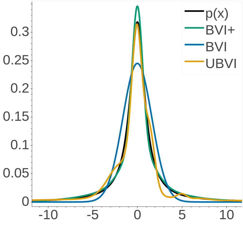
(a) Cauchy density

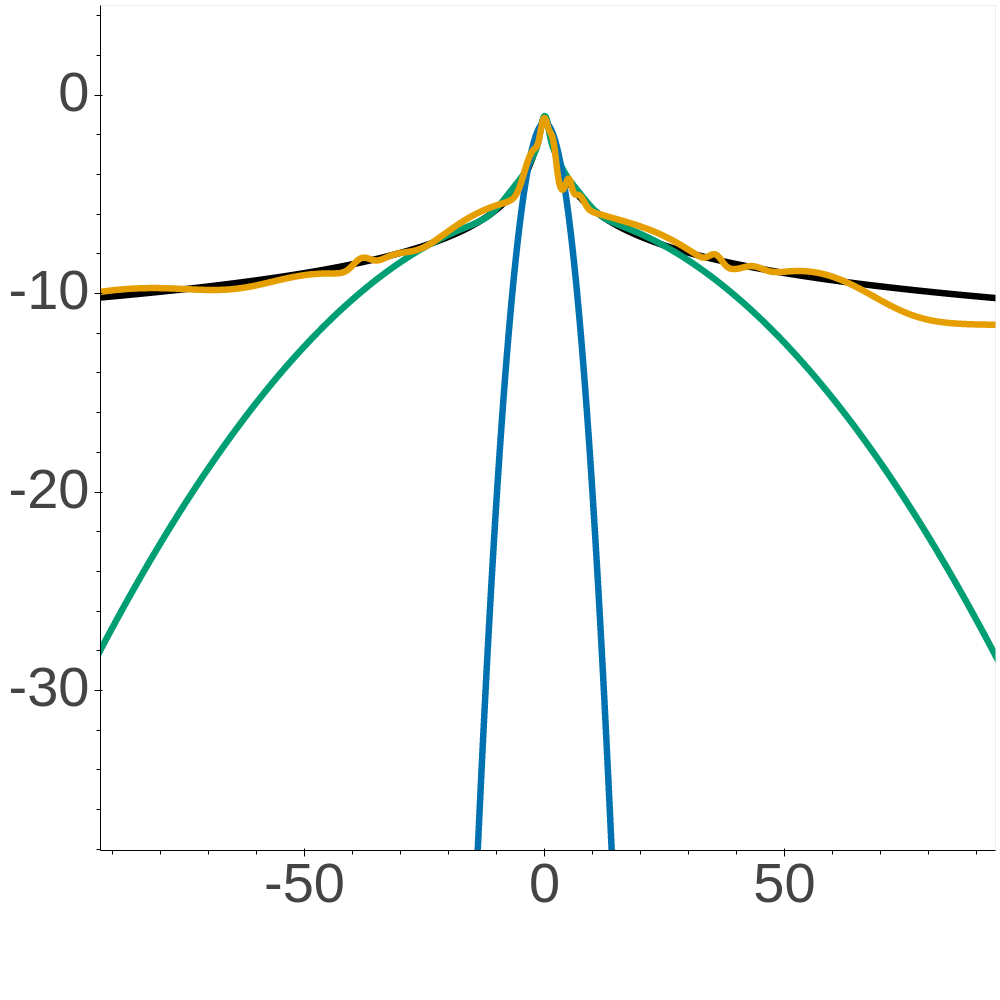
(b) Cauchy log density

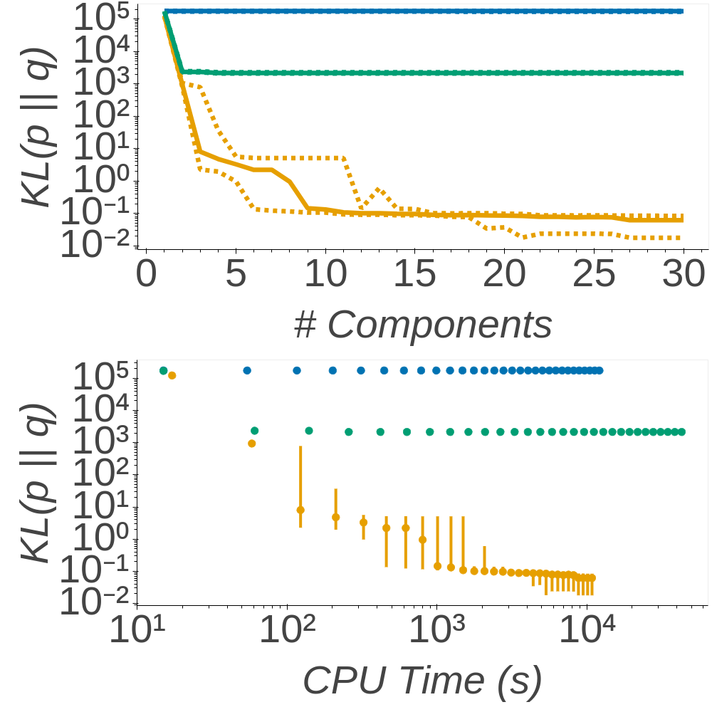
(c) Cauchy KL divergence

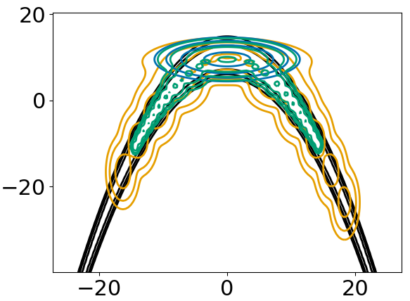
(d) Banana density

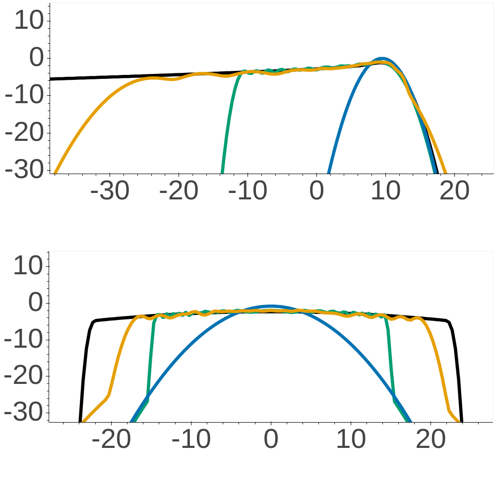
(e) Banana log marginal densities

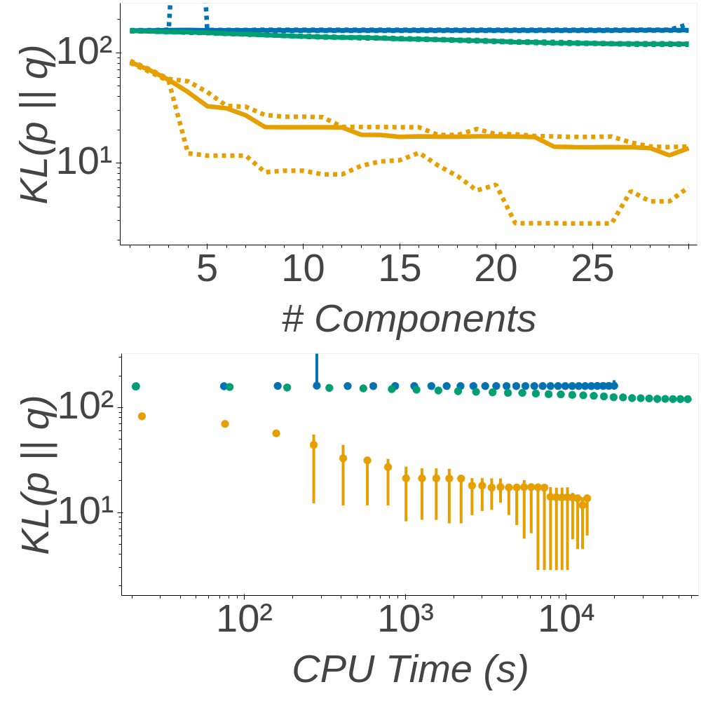
(f) Banana KL divergence

Figure 3: Results on the Cauchy and banana distributions; all subfigures use the legend from Fig. 3(a). (Figs. 3(a) and 3(d)): Density approximation with 30 components for Cauchy (3(a)) and banana (3(d)). BVI has degenerate component optimizations after the first, while UBVI and BVI+ are able to refine the approximation. (Figs. 3(b) and 3(e)): Log density approximations for Cauchy (3(b)) and banana marginals (3(e)). UBVI provides more accurate approximation of distribution tails than the KL-based BVI(+) algorithms. (Figs. 3(c) and 3(f)): The forward KL divergence vs. the number of boosting components and computation time. UBVI consistently improves its approximation as more components are added, while the KL-based BVI(+) methods improve either slowly or not at all due to degeneracy. Solid lines / dots indicate median, and dashed lines / whiskers indicate $25^{\text{th}}$ and $75^{\text{th}}$ percentile.

5.1 Cauchy and banana distributions

Fig. 3 shows the results of running UBVI, BVI, and BVI+ for 30 boosting iterations on the standard univariate Cauchy distribution and the banana distribution [56] with curvature $b=0.1$. These distributions were selected for their heavy tails and complex structure (shown in Figs. 3(b) and 3(e)), two features that standard variational inference does not often address but boosting methods should handle. However, BVI particularly struggles with heavy-tailed distributions, where its component optimization objective after the first is degenerate. BVI+ is able to refine its approximation, but still cannot capture heavy tails well, leading to large forward KL divergence (which controls downstream importance sampling error). We also found that the behaviour of BVI(+) is very sensitive to the choice of regularization tuning schedule $r_{n}$, and is difficult to tune well. UBVI, in contrast, approximates both heavy-tailed and complex distributions well with few components, and involves no tuning effort beyond the component optimization step size.

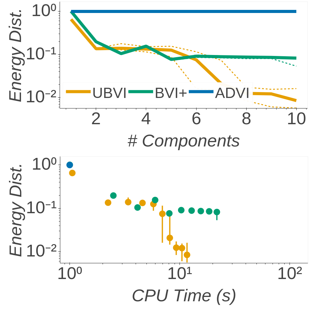
(a) Synthetic

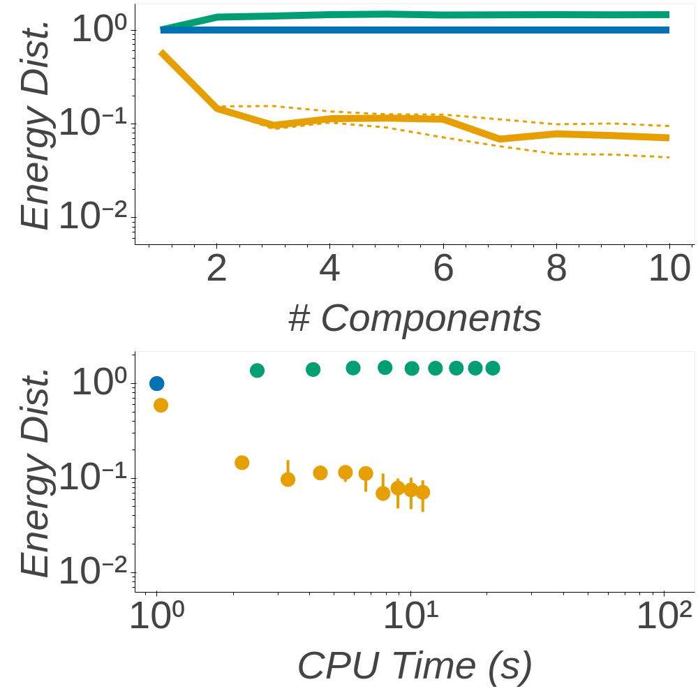
(b) Chemical Reactivity

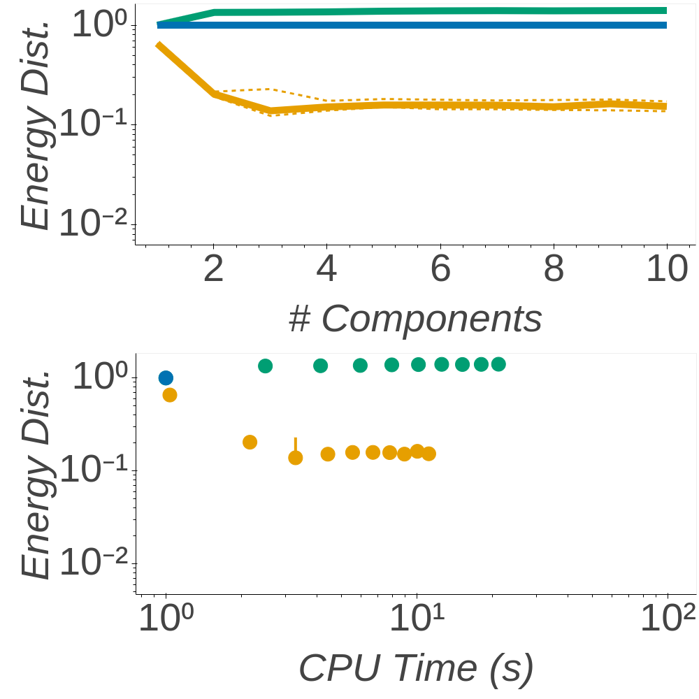
(c) Phishing

Figure 4: Results from Bayesian logistic regression posterior inference on the synthetic (4(a)), chemical (4(b)), and phishing (4(c)) datasets, showing the energy distance [57] to the posterior (via NUTS [58]) vs. the number of components and CPU time. Energy distance and time are normalized by the VI median. Solid lines / dots indicate median, and dashed lines / whiskers indicate $25^{\text{th}}$ / $75^{\text{th}}$ percentile.

5.2 Logistic regression with a heavy-tailed prior

Fig. 4 shows the results of running 10 boosting iterations of UBVI, BVI+, and standard VI for posterior inference in Bayesian logistic regression. We used a multivariate $\mathcal{T}_{2}(\mu,\Sigma)$ prior, where in each trial, the prior parameters were set via $\mu=0$ and $\Sigma=A^{T}A$ for $A_{ij}\overset{\textrm{\tiny{i.i.d.}\@}}{\sim}\mathcal{N}(0,1)$. We ran this experiment on a 2-dimensional synthetic dataset generated from the model, a 10-dimensional chemical reactivity dataset, and a 10-dimensional phishing websites dataset, each with 20 subsampled datapoints. The small dataset size and heavy-tailed prior were chosen to create a complex posterior structure better-suited to evaluating boosting variational methods. The results in Fig. 4 are similar to those in the synthetic test from Section 5.1; UBVI is able to refine its posterior approximation as it adds components without tuning effort, while the KL-based BVI+ method is difficult to tune well and does not reliably provide better posterior approximations than standard VI. BVI (no stabilization) is not shown, as its component optimizations after the first are degenerate and it reduces to standard VI.

6 Conclusion

This paper developed universal boosting variational inference (UBVI). UBVI optimizes the Hellinger metric, avoiding the degeneracy, tuning, and difficult joint component/weight optimizations of other gradient-based BVI methods, while simplifying fully-corrective weight optimizations. Theoretical guarantees on the convergence of Hellinger distance provide an MCMC-like computation/quality tradeoff, and experimental results demonstrate the advantages over previous variational methods.

7 Acknowledgments

T. Campbell and X. Li are supported by a National Sciences and Engineering Research Council of Canada (NSERC) Discovery Grant and an NSERC Discovery Launch Supplement.

Appendix A Component family and practical aspects of optimization

In order to use Algorithm 1, we need to compute or estimate $\left<h,\phi\right>$ for any $\phi\in L^{2}(\mu)$ and $\left<h,h^{\prime}\right>$ for any $h,h^{\prime}\in\mathcal{H}$. For arbitrary $\phi$, we use Monte Carlo estimates based on samples from $h^{2}$ via

$$\forall\phi\in L^{2}(\mu),\qquad\left<h,\phi\right> =\int h^{2}(x)\frac{\phi(x)}{h(x)}\mu(\mathrm{d}x)=\mathbb{E}_{h^{2}}\left[\frac{\phi(X)}{h(X)}\right]\approx\frac{1}{S}\sum_{s=1}^{S}\frac{\phi(X_{s})}{h(X_{s})}\quad X_{s}\overset{\textrm{\tiny{i.i.d.}\@}}{\sim}h^{2},$$ (27)

and employ an exponential component family $\mathcal{H}$ such that inner products $\left<h,h^{\prime}\right>$ between members of $\mathcal{H}$ are available in closed-form. In other words, for some base density $k(x)$, sufficient statistic $T(x)$, and log-partition $A(\eta)$, we let

$$\mathcal{H}=\left\{h_{\eta}\in L^{2}(\mu):h_{\eta}^{2}(x)=k(x)\exp\left(\eta^{T}T(x)-A(\eta)\right)\right\}.$$ (28)

Denoting $\eta_{i}$ to be the natural parameter for $g_{i}$, then $g_{i}=h_{\eta_{i}}$ and

$$Z_{ij}=\left<g_{i},g_{j}\right> =\int h_{\eta_{i}}(x)h_{\eta_{j}}(x)\mu(\mathrm{d}x)=\exp\left(A\left(\frac{\eta_{i}+\eta_{j}}{2}\right)-\frac{A(\eta_{i})+A(\eta_{j})}{2}\right).$$ (29)

In practice, we use a few techniques to improve the stability and performance of UBVI:

Component Initialization

The performance of variational boosting methods is often sensitive to the choice of initialization in each component optimization. The initialization used in this work is based on the intuition that after the first component optimization, each subsequent optimization will typically do one of two things: either it will find a new mode, or it will attempt to refine a previously found mode. If we wish to refine a previous mode, it is useful to initialize the optimization near that mode with a similar covariance structure. If we wish to discover a new mode, it is preferable to sample an initialization from the present distribution with significant added noise. In the experimental section of this work, we take the middle ground. We first sample a component from the current mixture approximation. Then, we generate an initialization for the Gaussian mean by sampling from that component with its covariance increased by a factor of 16. Finally, we initialize the covariance by using that component’s covariance multiplied by a standard log-normal random variable.

Objective Transformation

We maximize $\log(J(x))\mathds{1}\left[J(x)\geq 0\right]-\log(-J(x))\mathds{1}\left[J(x)<0\right]$, where $J(x)$ is the objective in Eq. 15, to avoid vanishing gradients and handle possible negativity; while this technically makes the Monte Carlo-based stochastic gradient estimates biased, it significantly improves performance in practice.

Parametrization

The choice of parametrization can have a significant effect on the conditioning of the optimization problem. Although we exploit the properties of the exponential family for $Z_{ij}$ evaluation in Eq. 29, we do not use the natural parametrization during optimization. In particular, we optimize over the mean and log-transformed marginal variances $\log\sigma_{i}^{2}$ in the diagonal covariance matrix $\Sigma=\operatorname{diag}(\sigma_{1}^{2},\dots,\sigma_{D}^{2})$.

Large-Scale Data

If the target density $p$ arises from a Bayesian posterior inference problem with a large dataset, computing $p$ and its gradients exactly in each component optimization iteration is expensive. Thus, one can use a Monte Carlo minibatch approximation with uniformly subsampled data per [50].

Estimating $\left<f,g\right>$

We use different numbers of samples for the component optimization stochastic gradient estimates and the estimates of $\left<f,g_{n}\right>$ (Line 9, Algorithm 1) required to solve the UBVI weight optimization. In particular, we use a relatively high number of samples (10,000 in our experiments) for estimating $\left<f,g_{n}\right>$, as these each need to be estimated only once, and they have a high impact on the choice of weights and thus future components; and for stochastic optimization, we use a lower number of samples (1,000 in our experiments) to avoid overly expensive component optimizations.

Appendix B Proofs

B.1 Proof of gradient boosting BVI behaviour

Proof of Proposition 1.

Let $\phi(x;\sigma^{2})$ be the normal density with mean $0$ and variance $\sigma^{2}$. Then Eq. 6 is

$$\sigma^{\star 2}= \operatornamewithlimits{arg\,min}_{\sigma^{2}}\int\phi(x;\sigma^{2})\log\frac{\phi(x;\sigma^{2})^{r_{2}}\phi(x;\tau^{2})}{\phi(x;1)}\mathrm{d}x$$ (30)

$$= \operatornamewithlimits{arg\,min}_{\sigma^{2}}-r_{2}\log\sigma-\frac{\sigma^{2}}{2\tau^{2}}+\frac{\sigma^{2}}{2}$$ (31)

$$= \left\{\begin{array}[]{ll}\infty&\tau^{2}\leq 1\\ \frac{r_{2}\tau^{2}}{\tau^{2}-1}&\tau^{2}>1.\end{array}\right.$$ (34)

Therefore, if the initialization has variance $\tau^{2}\leq 1$ the component optimization is degenerate. Note that for any two variances $\sigma_{1}^{2}$, $\sigma_{2}^{2}$, the weight optimization is

$$w^{\star} =\operatornamewithlimits{arg\,min}_{w\in[0,1]}\int\left(w\phi(x;\sigma_{1}^{2})+(1-w)\phi(x;\sigma_{2}^{2})\right)\log\frac{\left(w\phi(x;\sigma_{1}^{2})+(1-w)\phi(x;\sigma_{2}^{2})\right)}{\phi(x;1)}\mathrm{d}x$$ (35)

$$=\operatornamewithlimits{arg\,min}_{w\in[0,1]}w\frac{\sigma_{1}^{2}}{2}-w\frac{\sigma_{2}^{2}}{2}+\int\left(w\phi(x;\sigma_{1}^{2})+(1-w)\phi(x;\sigma_{2}^{2})\right)\log\left(w\phi(x;\sigma_{1}^{2})+(1-w)\phi(x;\sigma_{2}^{2})\right)\mathrm{d}x,$$ (36)

and taking first and second derivatives,

$$\frac{\mathrm{d}}{\mathrm{d}w} =\frac{\sigma_{1}^{2}-\sigma_{2}^{2}}{2}+\int\left(\phi(x;\sigma_{1}^{2})-\phi(x;\sigma_{2}^{2})\right)\log\left(w\phi(x;\sigma_{1}^{2})+(1-w)\phi(x;\sigma_{2}^{2})\right)\mathrm{d}x$$ (37)

$$\frac{\mathrm{d}^{2}}{\mathrm{d}w^{2}} =\int\frac{\big{(}\phi(x;\sigma_{1}^{2})-\phi(x;\sigma_{2}^{2})\big{)}^{2}}{w\phi(x;\sigma_{1}^{2})+(1-w)\phi(x;\sigma_{2}^{2})}\mathrm{d}x>0$$ (38)

At $w=1$, $\int\left(\phi(x;\sigma_{1}^{2})-\phi(x;\sigma_{2}^{2})\right)\log\left(w\phi(x;\sigma_{1}^{2})+(1-w)\phi(x;\sigma_{2}^{2})\right)\mathrm{d}x=(\sigma_{2}^{2}-\sigma_{1}^{2})/(2\sigma_{1}^{2})$. Therefore, if $\sigma_{2}^{2}>\sigma_{1}^{2}>1$,

$$\frac{\mathrm{d}}{\mathrm{d}w}<\frac{\sigma_{1}^{2}-\sigma_{2}^{2}}{2}+\frac{\sigma_{2}^{2}-\sigma_{1}^{2}}{2\sigma_{1}^{2}}<0.$$ (39)

In other words, the derivative is always negative, so the optimization sets $w=1$ and forgets the new component. This situation occurs if $\sigma_{1}^{2}=\tau^{2}>1$, $\sigma_{2}^{2}=r_{2}\frac{\tau^{2}}{\tau^{2}-1}$ and $r_{2}>\tau^{2}-1$. ∎

Proof of Proposition 2.

Using the notation from the proof of Proposition 1, Eq. 6 is

$$\sigma^{\star 2}= \operatornamewithlimits{arg\,min}_{\sigma^{2}}\int\phi(x;\sigma^{2})\log\frac{\phi(x;\sigma^{2})^{r_{1}}}{\mathrm{Cauchy}(x;0,1)}\mathrm{d}x$$ (40)

$$= \operatornamewithlimits{arg\,min}_{\sigma^{2}}-\frac{1}{2}r_{1}\log\sigma^{2}+\mathbb{E}_{\mathcal{N}(0,1)}\left[\log(1+\sigma^{2}x^{2})\right].$$ (41)

Taking the derivative with respect to $\sigma^{2}$ followed by Jensen’s inequality yields

$$\frac{\mathrm{d}}{\mathrm{d}\sigma^{2}} =\sigma^{-2}\left(-\frac{1}{2}r_{1}+\mathbb{E}_{\mathcal{N}(0,1)}\left[\frac{\sigma^{2}x^{2}}{1+\sigma^{2}x^{2}}\right]\right)$$ (42)

$$\leq\sigma^{-2}\left(-\frac{1}{2}r_{1}+\frac{\sigma^{2}}{1+\sigma^{2}}\right).$$ (43)

Therefore if $r_{1}\geq 2$, the derivative with respect to $\sigma^{2}$ is always negative, so $\sigma^{2}$ increases without bound. ∎

B.2 Proofs of Hellinger distance properties

Proof of Proposition 4.

This follows from

$$\mathrm{D^{2}_{H}}\left(p,q\right)=\frac{1}{2}\int(f(x)-g(x))^{2}\mu(\mathrm{d}x) \leq\frac{1}{2}\int\left|f(x)-g(x)\right|(f(x)+g(x))\mu(\mathrm{d}x)$$ (44)

$$=\frac{1}{2}\int\left|f^{2}(x)-g^{2}(x)\right|\mu(\mathrm{d}x)=\mathrm{D_{TV}}\left(p,q\right)$$ (45)

and

$$\mathrm{D_{TV}}\left(p,q\right) =\frac{1}{2}\int\left|f^{2}(x)-g^{2}(x)\right|\mu(\mathrm{d}x)$$ (46)

$$=\frac{1}{2}\int|f(x)-g(x)|(f(x)+g(x))\mu(\mathrm{d}x)$$ (47)

$$\leq\frac{1}{2}\mathchoice{{\hbox{$\displaystyle\sqrt{\int|f(x)-g(x)|^{2}\mu(\mathrm{d}x)\int(f(x)+g(x))^{2}\mu(\mathrm{d}x)\,}$}\lower 0.4pt\hbox{\vrule height=8.374pt,depth=-6.69923pt}}}{{\hbox{$\textstyle\sqrt{\int|f(x)-g(x)|^{2}\mu(\mathrm{d}x)\int(f(x)+g(x))^{2}\mu(\mathrm{d}x)\,}$}\lower 0.4pt\hbox{\vrule height=8.374pt,depth=-6.69923pt}}}{{\hbox{$\scriptstyle\sqrt{\int|f(x)-g(x)|^{2}\mu(\mathrm{d}x)\int(f(x)+g(x))^{2}\mu(\mathrm{d}x)\,}$}\lower 0.4pt\hbox{\vrule height=5.885pt,depth=-4.70802pt}}}{{\hbox{$\scriptscriptstyle\sqrt{\int|f(x)-g(x)|^{2}\mu(\mathrm{d}x)\int(f(x)+g(x))^{2}\mu(\mathrm{d}x)\,}$}\lower 0.4pt\hbox{\vrule height=4.535pt,depth=-3.62802pt}}}$$ (48)

$$=\frac{1}{\mathchoice{{\hbox{$\displaystyle\sqrt{2\,}$}\lower 0.4pt\hbox{\vrule height=5.79999pt,depth=-4.64001pt}}}{{\hbox{$\textstyle\sqrt{2\,}$}\lower 0.4pt\hbox{\vrule height=5.79999pt,depth=-4.64001pt}}}{{\hbox{$\scriptstyle\sqrt{2\,}$}\lower 0.4pt\hbox{\vrule height=4.06pt,depth=-3.24802pt}}}{{\hbox{$\scriptscriptstyle\sqrt{2\,}$}\lower 0.4pt\hbox{\vrule height=2.9pt,depth=-2.32pt}}}}\mathrm{D_{H}}\left(p,q\right)\mathchoice{{\hbox{$\displaystyle\sqrt{2+2\int f(x)g(x)\mu(\mathrm{d}x)\,}$}\lower 0.4pt\hbox{\vrule height=6.75pt,depth=-5.40002pt}}}{{\hbox{$\textstyle\sqrt{2+2\int f(x)g(x)\mu(\mathrm{d}x)\,}$}\lower 0.4pt\hbox{\vrule height=6.75pt,depth=-5.40002pt}}}{{\hbox{$\scriptstyle\sqrt{2+2\int f(x)g(x)\mu(\mathrm{d}x)\,}$}\lower 0.4pt\hbox{\vrule height=4.72499pt,depth=-3.78001pt}}}{{\hbox{$\scriptscriptstyle\sqrt{2+2\int f(x)g(x)\mu(\mathrm{d}x)\,}$}\lower 0.4pt\hbox{\vrule height=3.375pt,depth=-2.70001pt}}}$$ (49)

$$=\mathrm{D_{H}}\left(p,q\right)\mathchoice{{\hbox{$\displaystyle\sqrt{2-\mathrm{D^{2}_{H}}\left(p,q\right)\,}$}\lower 0.4pt\hbox{\vrule height=7.77397pt,depth=-6.21921pt}}}{{\hbox{$\textstyle\sqrt{2-\mathrm{D^{2}_{H}}\left(p,q\right)\,}$}\lower 0.4pt\hbox{\vrule height=7.77397pt,depth=-6.21921pt}}}{{\hbox{$\scriptstyle\sqrt{2-\mathrm{D^{2}_{H}}\left(p,q\right)\,}$}\lower 0.4pt\hbox{\vrule height=5.465pt,depth=-4.37202pt}}}{{\hbox{$\scriptscriptstyle\sqrt{2-\mathrm{D^{2}_{H}}\left(p,q\right)\,}$}\lower 0.4pt\hbox{\vrule height=4.23499pt,depth=-3.38802pt}}}.$$ (50)

∎

Proof of Proposition 5.

Combining a bound on the $\ell$-Wasserstein distance [51, Theorem 6.15],

$$W^{\ell}_{\ell}(p,q) \leq 2^{\ell-1}\int d(x_{0},x)^{\ell}\left|p(x)-q(x)\right|\mu(\mathrm{d}x),$$ (51)

with $|p(x)-q(x)|=|\mathchoice{{\hbox{$\displaystyle\sqrt{p(x)\,}$}\lower 0.4pt\hbox{\vrule height=6.75pt,depth=-5.40002pt}}}{{\hbox{$\textstyle\sqrt{p(x)\,}$}\lower 0.4pt\hbox{\vrule height=6.75pt,depth=-5.40002pt}}}{{\hbox{$\scriptstyle\sqrt{p(x)\,}$}\lower 0.4pt\hbox{\vrule height=4.72499pt,depth=-3.78001pt}}}{{\hbox{$\scriptscriptstyle\sqrt{p(x)\,}$}\lower 0.4pt\hbox{\vrule height=3.375pt,depth=-2.70001pt}}}-\mathchoice{{\hbox{$\displaystyle\sqrt{q(x)\,}$}\lower 0.4pt\hbox{\vrule height=6.75pt,depth=-5.40002pt}}}{{\hbox{$\textstyle\sqrt{q(x)\,}$}\lower 0.4pt\hbox{\vrule height=6.75pt,depth=-5.40002pt}}}{{\hbox{$\scriptstyle\sqrt{q(x)\,}$}\lower 0.4pt\hbox{\vrule height=4.72499pt,depth=-3.78001pt}}}{{\hbox{$\scriptscriptstyle\sqrt{q(x)\,}$}\lower 0.4pt\hbox{\vrule height=3.375pt,depth=-2.70001pt}}}|(\mathchoice{{\hbox{$\displaystyle\sqrt{p(x)\,}$}\lower 0.4pt\hbox{\vrule height=6.75pt,depth=-5.40002pt}}}{{\hbox{$\textstyle\sqrt{p(x)\,}$}\lower 0.4pt\hbox{\vrule height=6.75pt,depth=-5.40002pt}}}{{\hbox{$\scriptstyle\sqrt{p(x)\,}$}\lower 0.4pt\hbox{\vrule height=4.72499pt,depth=-3.78001pt}}}{{\hbox{$\scriptscriptstyle\sqrt{p(x)\,}$}\lower 0.4pt\hbox{\vrule height=3.375pt,depth=-2.70001pt}}}+\mathchoice{{\hbox{$\displaystyle\sqrt{q(x)\,}$}\lower 0.4pt\hbox{\vrule height=6.75pt,depth=-5.40002pt}}}{{\hbox{$\textstyle\sqrt{q(x)\,}$}\lower 0.4pt\hbox{\vrule height=6.75pt,depth=-5.40002pt}}}{{\hbox{$\scriptstyle\sqrt{q(x)\,}$}\lower 0.4pt\hbox{\vrule height=4.72499pt,depth=-3.78001pt}}}{{\hbox{$\scriptscriptstyle\sqrt{q(x)\,}$}\lower 0.4pt\hbox{\vrule height=3.375pt,depth=-2.70001pt}}})$, Cauchy-Schwarz, and Proposition 4 implies

$$W^{\ell}_{\ell}(p,q) \leq 2^{\ell-1/2}\mathrm{D_{H}}\left(p,q\right)\mathchoice{{\hbox{$\displaystyle\sqrt{\int d(x_{0},x)^{2\ell}\left(\mathchoice{{\hbox{$\displaystyle\sqrt{p(x)\,}$}\lower 0.4pt\hbox{\vrule height=6.75pt,depth=-5.40002pt}}}{{\hbox{$\textstyle\sqrt{p(x)\,}$}\lower 0.4pt\hbox{\vrule height=6.75pt,depth=-5.40002pt}}}{{\hbox{$\scriptstyle\sqrt{p(x)\,}$}\lower 0.4pt\hbox{\vrule height=4.72499pt,depth=-3.78001pt}}}{{\hbox{$\scriptscriptstyle\sqrt{p(x)\,}$}\lower 0.4pt\hbox{\vrule height=3.375pt,depth=-2.70001pt}}}+\mathchoice{{\hbox{$\displaystyle\sqrt{q(x)\,}$}\lower 0.4pt\hbox{\vrule height=6.75pt,depth=-5.40002pt}}}{{\hbox{$\textstyle\sqrt{q(x)\,}$}\lower 0.4pt\hbox{\vrule height=6.75pt,depth=-5.40002pt}}}{{\hbox{$\scriptstyle\sqrt{q(x)\,}$}\lower 0.4pt\hbox{\vrule height=4.72499pt,depth=-3.78001pt}}}{{\hbox{$\scriptscriptstyle\sqrt{q(x)\,}$}\lower 0.4pt\hbox{\vrule height=3.375pt,depth=-2.70001pt}}}\right)^{2}\mu(\mathrm{d}x)\,}$}\lower 0.4pt\hbox{\vrule height=8.5pt,depth=-6.80003pt}}}{{\hbox{$\textstyle\sqrt{\int d(x_{0},x)^{2\ell}\left(\mathchoice{{\hbox{$\displaystyle\sqrt{p(x)\,}$}\lower 0.4pt\hbox{\vrule height=6.75pt,depth=-5.40002pt}}}{{\hbox{$\textstyle\sqrt{p(x)\,}$}\lower 0.4pt\hbox{\vrule height=6.75pt,depth=-5.40002pt}}}{{\hbox{$\scriptstyle\sqrt{p(x)\,}$}\lower 0.4pt\hbox{\vrule height=4.72499pt,depth=-3.78001pt}}}{{\hbox{$\scriptscriptstyle\sqrt{p(x)\,}$}\lower 0.4pt\hbox{\vrule height=3.375pt,depth=-2.70001pt}}}+\mathchoice{{\hbox{$\displaystyle\sqrt{q(x)\,}$}\lower 0.4pt\hbox{\vrule height=6.75pt,depth=-5.40002pt}}}{{\hbox{$\textstyle\sqrt{q(x)\,}$}\lower 0.4pt\hbox{\vrule height=6.75pt,depth=-5.40002pt}}}{{\hbox{$\scriptstyle\sqrt{q(x)\,}$}\lower 0.4pt\hbox{\vrule height=4.72499pt,depth=-3.78001pt}}}{{\hbox{$\scriptscriptstyle\sqrt{q(x)\,}$}\lower 0.4pt\hbox{\vrule height=3.375pt,depth=-2.70001pt}}}\right)^{2}\mu(\mathrm{d}x)\,}$}\lower 0.4pt\hbox{\vrule height=8.5pt,depth=-6.80003pt}}}{{\hbox{$\scriptstyle\sqrt{\int d(x_{0},x)^{2\ell}\left(\mathchoice{{\hbox{$\displaystyle\sqrt{p(x)\,}$}\lower 0.4pt\hbox{\vrule height=4.72499pt,depth=-3.78001pt}}}{{\hbox{$\textstyle\sqrt{p(x)\,}$}\lower 0.4pt\hbox{\vrule height=4.72499pt,depth=-3.78001pt}}}{{\hbox{$\scriptstyle\sqrt{p(x)\,}$}\lower 0.4pt\hbox{\vrule height=3.3075pt,depth=-2.64601pt}}}{{\hbox{$\scriptscriptstyle\sqrt{p(x)\,}$}\lower 0.4pt\hbox{\vrule height=2.36249pt,depth=-1.89pt}}}+\mathchoice{{\hbox{$\displaystyle\sqrt{q(x)\,}$}\lower 0.4pt\hbox{\vrule height=4.72499pt,depth=-3.78001pt}}}{{\hbox{$\textstyle\sqrt{q(x)\,}$}\lower 0.4pt\hbox{\vrule height=4.72499pt,depth=-3.78001pt}}}{{\hbox{$\scriptstyle\sqrt{q(x)\,}$}\lower 0.4pt\hbox{\vrule height=3.3075pt,depth=-2.64601pt}}}{{\hbox{$\scriptscriptstyle\sqrt{q(x)\,}$}\lower 0.4pt\hbox{\vrule height=2.36249pt,depth=-1.89pt}}}\right)^{2}\mu(\mathrm{d}x)\,}$}\lower 0.4pt\hbox{\vrule height=5.97499pt,depth=-4.78001pt}}}{{\hbox{$\scriptscriptstyle\sqrt{\int d(x_{0},x)^{2\ell}\left(\mathchoice{{\hbox{$\displaystyle\sqrt{p(x)\,}$}\lower 0.4pt\hbox{\vrule height=3.375pt,depth=-2.70001pt}}}{{\hbox{$\textstyle\sqrt{p(x)\,}$}\lower 0.4pt\hbox{\vrule height=3.375pt,depth=-2.70001pt}}}{{\hbox{$\scriptstyle\sqrt{p(x)\,}$}\lower 0.4pt\hbox{\vrule height=2.36249pt,depth=-1.89pt}}}{{\hbox{$\scriptscriptstyle\sqrt{p(x)\,}$}\lower 0.4pt\hbox{\vrule height=1.6875pt,depth=-1.35pt}}}+\mathchoice{{\hbox{$\displaystyle\sqrt{q(x)\,}$}\lower 0.4pt\hbox{\vrule height=3.375pt,depth=-2.70001pt}}}{{\hbox{$\textstyle\sqrt{q(x)\,}$}\lower 0.4pt\hbox{\vrule height=3.375pt,depth=-2.70001pt}}}{{\hbox{$\scriptstyle\sqrt{q(x)\,}$}\lower 0.4pt\hbox{\vrule height=2.36249pt,depth=-1.89pt}}}{{\hbox{$\scriptscriptstyle\sqrt{q(x)\,}$}\lower 0.4pt\hbox{\vrule height=1.6875pt,depth=-1.35pt}}}\right)^{2}\mu(\mathrm{d}x)\,}$}\lower 0.4pt\hbox{\vrule height=4.625pt,depth=-3.70003pt}}}.$$ (52)

Finally, since $(a+b)^{2}\leq 2a^{2}+2b^{2}$ for $a,b\in\mathbb{R}$,

$$W^{\ell}_{\ell}(p,q) \leq 2^{\ell}\mathrm{D_{H}}\left(p,q\right)\mathchoice{{\hbox{$\displaystyle\sqrt{\int d(x_{0},x)^{2\ell}(p(x)+q(x))\mu(\mathrm{d}x)\,}$}\lower 0.4pt\hbox{\vrule height=8.5pt,depth=-6.80003pt}}}{{\hbox{$\textstyle\sqrt{\int d(x_{0},x)^{2\ell}(p(x)+q(x))\mu(\mathrm{d}x)\,}$}\lower 0.4pt\hbox{\vrule height=8.5pt,depth=-6.80003pt}}}{{\hbox{$\scriptstyle\sqrt{\int d(x_{0},x)^{2\ell}(p(x)+q(x))\mu(\mathrm{d}x)\,}$}\lower 0.4pt\hbox{\vrule height=5.97499pt,depth=-4.78001pt}}}{{\hbox{$\scriptscriptstyle\sqrt{\int d(x_{0},x)^{2\ell}(p(x)+q(x))\mu(\mathrm{d}x)\,}$}\lower 0.4pt\hbox{\vrule height=4.625pt,depth=-3.70003pt}}}.$$ (53)

∎

Proof of Proposition 6.

Rearranging the definition of Hellinger distance squared,

$$\mathrm{D^{2}_{H}}\left(p,q\right) =\frac{1}{2}\int\left(\mathchoice{{\hbox{$\displaystyle\sqrt{p(x)\,}$}\lower 0.4pt\hbox{\vrule height=6.75pt,depth=-5.40002pt}}}{{\hbox{$\textstyle\sqrt{p(x)\,}$}\lower 0.4pt\hbox{\vrule height=6.75pt,depth=-5.40002pt}}}{{\hbox{$\scriptstyle\sqrt{p(x)\,}$}\lower 0.4pt\hbox{\vrule height=4.72499pt,depth=-3.78001pt}}}{{\hbox{$\scriptscriptstyle\sqrt{p(x)\,}$}\lower 0.4pt\hbox{\vrule height=3.375pt,depth=-2.70001pt}}}-\mathchoice{{\hbox{$\displaystyle\sqrt{q(x)\,}$}\lower 0.4pt\hbox{\vrule height=6.75pt,depth=-5.40002pt}}}{{\hbox{$\textstyle\sqrt{q(x)\,}$}\lower 0.4pt\hbox{\vrule height=6.75pt,depth=-5.40002pt}}}{{\hbox{$\scriptstyle\sqrt{q(x)\,}$}\lower 0.4pt\hbox{\vrule height=4.72499pt,depth=-3.78001pt}}}{{\hbox{$\scriptscriptstyle\sqrt{q(x)\,}$}\lower 0.4pt\hbox{\vrule height=3.375pt,depth=-2.70001pt}}}\right)^{2}\mu(\mathrm{d}x)$$ (54)

$$=\frac{1}{2}\int p(x)\frac{q(x)}{p(x)}\left(\mathchoice{{\hbox{$\displaystyle\sqrt{\frac{p(x)}{q(x)}\,}$}\lower 0.4pt\hbox{\vrule height=13.5pt,depth=-10.80005pt}}}{{\hbox{$\textstyle\sqrt{\frac{p(x)}{q(x)}\,}$}\lower 0.4pt\hbox{\vrule height=9.44998pt,depth=-7.56003pt}}}{{\hbox{$\scriptstyle\sqrt{\frac{p(x)}{q(x)}\,}$}\lower 0.4pt\hbox{\vrule height=6.75pt,depth=-5.40002pt}}}{{\hbox{$\scriptscriptstyle\sqrt{\frac{p(x)}{q(x)}\,}$}\lower 0.4pt\hbox{\vrule height=6.75pt,depth=-5.40002pt}}}-1\right)^{2}\mu(\mathrm{d}x).$$ (55)

For $x>1$, $x^{-1}\left(\mathchoice{{\hbox{$\displaystyle\sqrt{x\,}$}\lower 0.4pt\hbox{\vrule height=3.87498pt,depth=-3.1pt}}}{{\hbox{$\textstyle\sqrt{x\,}$}\lower 0.4pt\hbox{\vrule height=3.87498pt,depth=-3.1pt}}}{{\hbox{$\scriptstyle\sqrt{x\,}$}\lower 0.4pt\hbox{\vrule height=2.7125pt,depth=-2.17001pt}}}{{\hbox{$\scriptscriptstyle\sqrt{x\,}$}\lower 0.4pt\hbox{\vrule height=1.93748pt,depth=-1.55pt}}}-1\right)^{2}\geq\left(\frac{\log x}{1+\log x}\right)^{2}$, and for $x\leq 1$, $x^{-1}\left(\mathchoice{{\hbox{$\displaystyle\sqrt{x\,}$}\lower 0.4pt\hbox{\vrule height=3.87498pt,depth=-3.1pt}}}{{\hbox{$\textstyle\sqrt{x\,}$}\lower 0.4pt\hbox{\vrule height=3.87498pt,depth=-3.1pt}}}{{\hbox{$\scriptstyle\sqrt{x\,}$}\lower 0.4pt\hbox{\vrule height=2.7125pt,depth=-2.17001pt}}}{{\hbox{$\scriptscriptstyle\sqrt{x\,}$}\lower 0.4pt\hbox{\vrule height=1.93748pt,depth=-1.55pt}}}-1\right)^{2}\geq\left(\log x\right)^{2}$, so

$$\mathrm{D^{2}_{H}}\left(p,q\right) \geq\frac{1}{2}\int_{p>q}p(x)\left(\frac{\log\frac{p(x)}{q(x)}}{1+\log\frac{p(x)}{q(x)}}\right)^{2}\mu(\mathrm{d}x)+\frac{1}{2}\int_{p\leq q}p(x)\left(\log\frac{p(x)}{q(x)}\right)^{2}\mu(\mathrm{d}x).$$ (56)

Now using the relation $2a^{2}+2b^{2}\geq(a+b)^{2}$,

$$\mathrm{D^{2}_{H}}\left(p,q\right) \geq\frac{1}{4}\int p(x)\left(\mathds{1}\left[p>q\right]\frac{\log\frac{p(x)}{q(x)}}{1+\log\frac{p(x)}{q(x)}}+\mathds{1}\left[p\leq q\right]\log\frac{p(x)}{q(x)}\right)^{2}\mu(\mathrm{d}x)$$ (57)

$$=\frac{1}{4}\int p(x)\left(\frac{\mathds{1}\left[p>q\right]\log\frac{p(x)}{q(x)}+\mathds{1}\left[p\leq q\right]\log\frac{p(x)}{q(x)}\left(1+\log\frac{p(x)}{q(x)}\right)}{1+\log\frac{p(x)}{q(x)}}\right)^{2}\mu(\mathrm{d}x)$$ (58)

$$=\frac{1}{4}\int p(x)\left(\log\frac{p(x)}{q(x)}\right)^{2}\left(\frac{1+\mathds{1}\left[\log\frac{p(x)}{q(x)}\leq 0\right]\log\frac{p(x)}{q(x)}}{1+\log\frac{p(x)}{q(x)}}\right)^{2}\mu(\mathrm{d}x).$$ (59)

This provides the first result. Using the reverse Hölder inequality $\|fg\|_{1}\geq\|f\|_{\frac{1}{p}}\|g\|_{\frac{-1}{p-1}}$ for $p=2\in(1,\infty)$,

$$\mathrm{D^{2}_{H}}\left(p,q\right) \geq\frac{1}{4}\left(\int p(x)\log\frac{p(x)}{q(x)}\mu(\mathrm{d}x)\right)^{2}\left(\int p(x)\left(\frac{1+\log\frac{p(x)}{q(x)}}{1+\mathds{1}\left[\log\frac{p(x)}{q(x)}\leq 0\right]\log\frac{p(x)}{q(x)}}\right)^{2}\mu(\mathrm{d}x)\right)^{-1}$$ (60)

$$=\frac{1}{4}\mathrm{D^{2}_{KL}}\left(p||q\right)\left(\mathbb{P}\left(\log\frac{p(x)}{q(x)}\leq 0\right)+\int p(x)\mathds{1}\left[\log\frac{p(x)}{q(x)}>0\right]\left(1+\log\frac{p(x)}{q(x)}\right)^{2}\mu(\mathrm{d}x)\right)^{-1}$$ (61)

$$\geq\frac{1}{4}\mathrm{D^{2}_{KL}}\left(p||q\right)\left(1+\int p(x)\mathds{1}\left[\log\frac{p(x)}{q(x)}>0\right]\left(1+\log\frac{p(x)}{q(x)}\right)^{2}\mu(\mathrm{d}x)\right)^{-1}.$$ (62)

∎

Proof of Proposition 7.

This proof uses a technique adapted from [54, Theorem 1.1]. Let $Y\sim p(y)\mu(\mathrm{d}y)$, $X\sim q(x)\mu(\mathrm{d}x)$, and for $a\geq 0$,

$$\rho(x) :=\left|1-\mathchoice{{\hbox{$\displaystyle\sqrt{\frac{q(x)}{p(x)}\,}$}\lower 0.4pt\hbox{\vrule height=13.5pt,depth=-10.80005pt}}}{{\hbox{$\textstyle\sqrt{\frac{q(x)}{p(x)}\,}$}\lower 0.4pt\hbox{\vrule height=9.44998pt,depth=-7.56003pt}}}{{\hbox{$\scriptstyle\sqrt{\frac{q(x)}{p(x)}\,}$}\lower 0.4pt\hbox{\vrule height=6.75pt,depth=-5.40002pt}}}{{\hbox{$\scriptscriptstyle\sqrt{\frac{q(x)}{p(x)}\,}$}\lower 0.4pt\hbox{\vrule height=6.75pt,depth=-5.40002pt}}}\right|^{2} h(x) :=\phi(x)\mathds{1}\left[\rho(x)\leq a\right].$$ (63)

Then by Cauchy-Schwarz,

$$\mathbb{E}\left[\left|I_{n}(\phi)-I_{n}(h)\right|\right] \leq\|\phi\|_{L^{2}(p)}\mathchoice{{\hbox{$\displaystyle\sqrt{\mathbb{P}\left(\rho(Y)>a\right)\,}$}\lower 0.4pt\hbox{\vrule height=6.75pt,depth=-5.40002pt}}}{{\hbox{$\textstyle\sqrt{\mathbb{P}\left(\rho(Y)>a\right)\,}$}\lower 0.4pt\hbox{\vrule height=6.75pt,depth=-5.40002pt}}}{{\hbox{$\scriptstyle\sqrt{\mathbb{P}\left(\rho(Y)>a\right)\,}$}\lower 0.4pt\hbox{\vrule height=4.72499pt,depth=-3.78001pt}}}{{\hbox{$\scriptscriptstyle\sqrt{\mathbb{P}\left(\rho(Y)>a\right)\,}$}\lower 0.4pt\hbox{\vrule height=3.375pt,depth=-2.70001pt}}}$$ (64)

$$\left|I(\phi)-I(h)\right| \leq\|\phi\|_{L^{2}(p)}\mathchoice{{\hbox{$\displaystyle\sqrt{\mathbb{P}\left(\rho(Y)>a\right)\,}$}\lower 0.4pt\hbox{\vrule height=6.75pt,depth=-5.40002pt}}}{{\hbox{$\textstyle\sqrt{\mathbb{P}\left(\rho(Y)>a\right)\,}$}\lower 0.4pt\hbox{\vrule height=6.75pt,depth=-5.40002pt}}}{{\hbox{$\scriptstyle\sqrt{\mathbb{P}\left(\rho(Y)>a\right)\,}$}\lower 0.4pt\hbox{\vrule height=4.72499pt,depth=-3.78001pt}}}{{\hbox{$\scriptscriptstyle\sqrt{\mathbb{P}\left(\rho(Y)>a\right)\,}$}\lower 0.4pt\hbox{\vrule height=3.375pt,depth=-2.70001pt}}}$$ (65)

$$\mathbb{E}\left[\left|I_{n}(h)-I(h)\right|\right] \leq\mathchoice{{\hbox{$\displaystyle\sqrt{N\,}$}\lower 0.4pt\hbox{\vrule height=6.14998pt,depth=-4.92001pt}}}{{\hbox{$\textstyle\sqrt{N\,}$}\lower 0.4pt\hbox{\vrule height=6.14998pt,depth=-4.92001pt}}}{{\hbox{$\scriptstyle\sqrt{N\,}$}\lower 0.4pt\hbox{\vrule height=4.305pt,depth=-3.44402pt}}}{{\hbox{$\scriptscriptstyle\sqrt{N\,}$}\lower 0.4pt\hbox{\vrule height=3.07498pt,depth=-2.46pt}}}^{-1}\mathchoice{{\hbox{$\displaystyle\sqrt{\operatorname{Var}{\frac{p(X)}{q(X)}\phi(X)\mathds{1}\left[\rho(X)\leq a\right]}\,}$}\lower 0.4pt\hbox{\vrule height=13.5pt,depth=-10.80005pt}}}{{\hbox{$\textstyle\sqrt{\operatorname{Var}{\frac{p(X)}{q(X)}\phi(X)\mathds{1}\left[\rho(X)\leq a\right]}\,}$}\lower 0.4pt\hbox{\vrule height=9.44998pt,depth=-7.56003pt}}}{{\hbox{$\scriptstyle\sqrt{\operatorname{Var}{\frac{p(X)}{q(X)}\phi(X)\mathds{1}\left[\rho(X)\leq a\right]}\,}$}\lower 0.4pt\hbox{\vrule height=6.75pt,depth=-5.40002pt}}}{{\hbox{$\scriptscriptstyle\sqrt{\operatorname{Var}{\frac{p(X)}{q(X)}\phi(X)\mathds{1}\left[\rho(X)\leq a\right]}\,}$}\lower 0.4pt\hbox{\vrule height=6.75pt,depth=-5.40002pt}}}.$$ (66)

Now note that

$$\operatorname{Var}{\left(\frac{p(X)}{q(X)}\phi(X)\mathds{1}\left[\rho(X)\leq a\right]\right)} \leq\mathbb{E}\left[\frac{p^{2}(X)}{q^{2}(X)}\phi(X)^{2}\mathds{1}\left[\rho(X)\leq a\right]\right]$$ (67)

$$=\mathbb{E}\left[\frac{p(Y)}{q(Y)}\phi(Y)^{2}\mathds{1}\left[\rho(Y)\leq a\right]\right]$$ (68)

and for $a\in[0,1)$, $\rho(x)\leq a$ implies

$$\sqrt{\frac{q(x)}{p(x)}\,} \geq 1-\mathchoice{{\hbox{$\displaystyle\sqrt{a\,}$}\lower 0.4pt\hbox{\vrule height=3.87498pt,depth=-3.1pt}}}{{\hbox{$\textstyle\sqrt{a\,}$}\lower 0.4pt\hbox{\vrule height=3.87498pt,depth=-3.1pt}}}{{\hbox{$\scriptstyle\sqrt{a\,}$}\lower 0.4pt\hbox{\vrule height=2.7125pt,depth=-2.17001pt}}}{{\hbox{$\scriptscriptstyle\sqrt{a\,}$}\lower 0.4pt\hbox{\vrule height=1.93748pt,depth=-1.55pt}}}\implies\frac{p(x)}{q(x)}\leq(1-\mathchoice{{\hbox{$\displaystyle\sqrt{a\,}$}\lower 0.4pt\hbox{\vrule height=3.87498pt,depth=-3.1pt}}}{{\hbox{$\textstyle\sqrt{a\,}$}\lower 0.4pt\hbox{\vrule height=3.87498pt,depth=-3.1pt}}}{{\hbox{$\scriptstyle\sqrt{a\,}$}\lower 0.4pt\hbox{\vrule height=2.7125pt,depth=-2.17001pt}}}{{\hbox{$\scriptscriptstyle\sqrt{a\,}$}\lower 0.4pt\hbox{\vrule height=1.93748pt,depth=-1.55pt}}})^{-2}$$ (69)

So

$$\operatorname{Var}{\left(\frac{p(X)}{q(X)}\phi(X)\mathds{1}\left[\rho(X)\leq a\right]\right)} \leq\|\phi\|^{2}_{L^{2}(p)}\left(\frac{1}{(1-\mathchoice{{\hbox{$\displaystyle\sqrt{a\,}$}\lower 0.4pt\hbox{\vrule height=3.87498pt,depth=-3.1pt}}}{{\hbox{$\textstyle\sqrt{a\,}$}\lower 0.4pt\hbox{\vrule height=3.87498pt,depth=-3.1pt}}}{{\hbox{$\scriptstyle\sqrt{a\,}$}\lower 0.4pt\hbox{\vrule height=2.7125pt,depth=-2.17001pt}}}{{\hbox{$\scriptscriptstyle\sqrt{a\,}$}\lower 0.4pt\hbox{\vrule height=1.93748pt,depth=-1.55pt}}})^{2}}\right)$$ (70)

and hence

$$\mathbb{E}\left[\left|I_{n}(h)-I(h)\right|\right] \leq\|\phi\|_{L^{2}(p)}\mathchoice{{\hbox{$\displaystyle\sqrt{N\,}$}\lower 0.4pt\hbox{\vrule height=6.14998pt,depth=-4.92001pt}}}{{\hbox{$\textstyle\sqrt{N\,}$}\lower 0.4pt\hbox{\vrule height=6.14998pt,depth=-4.92001pt}}}{{\hbox{$\scriptstyle\sqrt{N\,}$}\lower 0.4pt\hbox{\vrule height=4.305pt,depth=-3.44402pt}}}{{\hbox{$\scriptscriptstyle\sqrt{N\,}$}\lower 0.4pt\hbox{\vrule height=3.07498pt,depth=-2.46pt}}}^{-1}\frac{1}{1-\mathchoice{{\hbox{$\displaystyle\sqrt{a\,}$}\lower 0.4pt\hbox{\vrule height=3.87498pt,depth=-3.1pt}}}{{\hbox{$\textstyle\sqrt{a\,}$}\lower 0.4pt\hbox{\vrule height=3.87498pt,depth=-3.1pt}}}{{\hbox{$\scriptstyle\sqrt{a\,}$}\lower 0.4pt\hbox{\vrule height=2.7125pt,depth=-2.17001pt}}}{{\hbox{$\scriptscriptstyle\sqrt{a\,}$}\lower 0.4pt\hbox{\vrule height=1.93748pt,depth=-1.55pt}}}}$$ (71)

By Markov’s inequality,

$$\mathbb{P}\left(\rho(Y)>a\right) \leq a^{-1}\mathbb{E}\left[\rho(Y)\right]=2a^{-1}\mathrm{D^{2}_{H}}\left(p,q\right).$$ (72)

So substituting and combining the three bounds from Eqs. 64, 65 and 66 using the triangle inequality,

$$\mathbb{E}\left[\left|I_{n}(\phi)-I(\phi)\right|\right] \leq\|\phi\|_{L^{2}(p)}\left(\frac{1}{\mathchoice{{\hbox{$\displaystyle\sqrt{N\,}$}\lower 0.4pt\hbox{\vrule height=6.14998pt,depth=-4.92001pt}}}{{\hbox{$\textstyle\sqrt{N\,}$}\lower 0.4pt\hbox{\vrule height=6.14998pt,depth=-4.92001pt}}}{{\hbox{$\scriptstyle\sqrt{N\,}$}\lower 0.4pt\hbox{\vrule height=4.305pt,depth=-3.44402pt}}}{{\hbox{$\scriptscriptstyle\sqrt{N\,}$}\lower 0.4pt\hbox{\vrule height=3.07498pt,depth=-2.46pt}}}(1-\mathchoice{{\hbox{$\displaystyle\sqrt{a\,}$}\lower 0.4pt\hbox{\vrule height=3.87498pt,depth=-3.1pt}}}{{\hbox{$\textstyle\sqrt{a\,}$}\lower 0.4pt\hbox{\vrule height=3.87498pt,depth=-3.1pt}}}{{\hbox{$\scriptstyle\sqrt{a\,}$}\lower 0.4pt\hbox{\vrule height=2.7125pt,depth=-2.17001pt}}}{{\hbox{$\scriptscriptstyle\sqrt{a\,}$}\lower 0.4pt\hbox{\vrule height=1.93748pt,depth=-1.55pt}}})}+\mathchoice{{\hbox{$\displaystyle\sqrt{8a^{-1}\,}$}\lower 0.4pt\hbox{\vrule height=5.79999pt,depth=-4.64001pt}}}{{\hbox{$\textstyle\sqrt{8a^{-1}\,}$}\lower 0.4pt\hbox{\vrule height=5.79999pt,depth=-4.64001pt}}}{{\hbox{$\scriptstyle\sqrt{8a^{-1}\,}$}\lower 0.4pt\hbox{\vrule height=4.06pt,depth=-3.24802pt}}}{{\hbox{$\scriptscriptstyle\sqrt{8a^{-1}\,}$}\lower 0.4pt\hbox{\vrule height=3.09749pt,depth=-2.47801pt}}}\mathrm{D_{H}}\left(p,q\right)\right).$$ (73)

Optimizing over $a$ yields

$$\mathchoice{{\hbox{$\displaystyle\sqrt{a\,}$}\lower 0.4pt\hbox{\vrule height=3.87498pt,depth=-3.1pt}}}{{\hbox{$\textstyle\sqrt{a\,}$}\lower 0.4pt\hbox{\vrule height=3.87498pt,depth=-3.1pt}}}{{\hbox{$\scriptstyle\sqrt{a\,}$}\lower 0.4pt\hbox{\vrule height=2.7125pt,depth=-2.17001pt}}}{{\hbox{$\scriptscriptstyle\sqrt{a\,}$}\lower 0.4pt\hbox{\vrule height=1.93748pt,depth=-1.55pt}}}=\frac{8^{1/4}\mathrm{D_{H}}\left(p,q\right)^{1/2}}{8^{1/4}\mathrm{D_{H}}\left(p,q\right)^{1/2}+N^{-1/4}},$$ (74)

and substituting with $8^{1/4}\leq 2$ yields

$$\mathbb{E}\left[\left|I_{n}(\phi)-I(\phi)\right|\right] \leq\|\phi\|_{L^{2}(p)}\left(N^{-\nicefrac{{1}}{{4}}}+2\mathchoice{{\hbox{$\displaystyle\sqrt{\mathrm{D_{H}}\left(p,q\right)\,}$}\lower 0.4pt\hbox{\vrule height=6.75pt,depth=-5.40002pt}}}{{\hbox{$\textstyle\sqrt{\mathrm{D_{H}}\left(p,q\right)\,}$}\lower 0.4pt\hbox{\vrule height=6.75pt,depth=-5.40002pt}}}{{\hbox{$\scriptstyle\sqrt{\mathrm{D_{H}}\left(p,q\right)\,}$}\lower 0.4pt\hbox{\vrule height=4.72499pt,depth=-3.78001pt}}}{{\hbox{$\scriptscriptstyle\sqrt{\mathrm{D_{H}}\left(p,q\right)\,}$}\lower 0.4pt\hbox{\vrule height=3.375pt,depth=-2.70001pt}}}\right)^{2}.$$ (75)

Setting $N=\alpha^{-4}\mathrm{D_{H}}\left(p,q\right)^{-2}$ yields the first result. For the second, note that $|I_{n}(\phi)-I(\phi)|\leq\|\phi\|_{L^{2}(p)}\delta$ and $|I_{n}(1)-1|\leq\eta$ implies that

$$\left|J_{n}(\phi)-I(\phi)\right|=\frac{\left|I_{n}(\phi)-I_{n}(1)I(\phi)\right|}{I_{n}(1)} \leq\frac{\left|I_{n}(\phi)-I(\phi)\right|+I(\phi)\left|I_{n}(1)-1\right|}{1-\left|I_{n}(1)-1\right|}$$ (76)

$$\leq\|\phi\|_{L^{2}(p)}\frac{\delta+\eta}{1-\eta},$$ (77)

so

$$\mathbb{P}\left(\left|J_{n}(\phi)-I(\phi)\right|>\|\phi\|_{L^{2}(p)}\frac{\delta+\eta}{1-\eta}\right) \leq\mathbb{P}\left(\left|I_{n}(\phi)-I(\phi)\right|>\|\phi\|_{L^{2}(p)}\delta\right)+\mathbb{P}\left(\left|I_{n}(\phi)-1\right|>\eta\right),$$ (78)

which by Markov inequality and the previous bound,

$$\mathbb{P}\left(\left|J_{n}(\phi)-I(\phi)\right|>\|\phi\|_{L^{2}(p)}\frac{\delta+\eta}{1-\eta}\right) \leq\left(N^{-\nicefrac{{1}}{{4}}}+2\mathchoice{{\hbox{$\displaystyle\sqrt{\mathrm{D_{H}}\left(p,q\right)\,}$}\lower 0.4pt\hbox{\vrule height=6.75pt,depth=-5.40002pt}}}{{\hbox{$\textstyle\sqrt{\mathrm{D_{H}}\left(p,q\right)\,}$}\lower 0.4pt\hbox{\vrule height=6.75pt,depth=-5.40002pt}}}{{\hbox{$\scriptstyle\sqrt{\mathrm{D_{H}}\left(p,q\right)\,}$}\lower 0.4pt\hbox{\vrule height=4.72499pt,depth=-3.78001pt}}}{{\hbox{$\scriptscriptstyle\sqrt{\mathrm{D_{H}}\left(p,q\right)\,}$}\lower 0.4pt\hbox{\vrule height=3.375pt,depth=-2.70001pt}}}\right)^{2}\left(\delta^{-1}+\eta^{-1}\right)$$ (79)

Minimizing $\delta^{-1}+\eta^{-1}$ subject to the constraint that $t=(\delta+\eta)/(1-\eta)$ yields the result. ∎

Proof of Proposition 8.

For the first bound, by Jensen’s inequality

$$\mathbb{E}\left[\left|\widehat{\mathrm{D^{2}_{H}}\left(p,q\right)}-\mathrm{D^{2}_{H}}\left(p,q\right)\right|\right] \leq\mathchoice{{\hbox{$\displaystyle\sqrt{\operatorname{Var}{\frac{1}{N}\sum_{n=1}^{N}\mathchoice{{\hbox{$\displaystyle\sqrt{\frac{p(X_{n})}{q(X_{n})}\,}$}\lower 0.4pt\hbox{\vrule height=13.5pt,depth=-10.80005pt}}}{{\hbox{$\textstyle\sqrt{\frac{p(X_{n})}{q(X_{n})}\,}$}\lower 0.4pt\hbox{\vrule height=9.44998pt,depth=-7.56003pt}}}{{\hbox{$\scriptstyle\sqrt{\frac{p(X_{n})}{q(X_{n})}\,}$}\lower 0.4pt\hbox{\vrule height=6.75pt,depth=-5.40002pt}}}{{\hbox{$\scriptscriptstyle\sqrt{\frac{p(X_{n})}{q(X_{n})}\,}$}\lower 0.4pt\hbox{\vrule height=6.75pt,depth=-5.40002pt}}}}\,}$}\lower 0.4pt\hbox{\vrule height=13.5pt,depth=-10.80005pt}}}{{\hbox{$\textstyle\sqrt{\operatorname{Var}{\frac{1}{N}\sum_{n=1}^{N}\mathchoice{{\hbox{$\displaystyle\sqrt{\frac{p(X_{n})}{q(X_{n})}\,}$}\lower 0.4pt\hbox{\vrule height=13.5pt,depth=-10.80005pt}}}{{\hbox{$\textstyle\sqrt{\frac{p(X_{n})}{q(X_{n})}\,}$}\lower 0.4pt\hbox{\vrule height=9.44998pt,depth=-7.56003pt}}}{{\hbox{$\scriptstyle\sqrt{\frac{p(X_{n})}{q(X_{n})}\,}$}\lower 0.4pt\hbox{\vrule height=6.75pt,depth=-5.40002pt}}}{{\hbox{$\scriptscriptstyle\sqrt{\frac{p(X_{n})}{q(X_{n})}\,}$}\lower 0.4pt\hbox{\vrule height=6.75pt,depth=-5.40002pt}}}}\,}$}\lower 0.4pt\hbox{\vrule height=13.5pt,depth=-10.80005pt}}}{{\hbox{$\scriptstyle\sqrt{\operatorname{Var}{\frac{1}{N}\sum_{n=1}^{N}\mathchoice{{\hbox{$\displaystyle\sqrt{\frac{p(X_{n})}{q(X_{n})}\,}$}\lower 0.4pt\hbox{\vrule height=9.44998pt,depth=-7.56003pt}}}{{\hbox{$\textstyle\sqrt{\frac{p(X_{n})}{q(X_{n})}\,}$}\lower 0.4pt\hbox{\vrule height=6.61497pt,depth=-5.292pt}}}{{\hbox{$\scriptstyle\sqrt{\frac{p(X_{n})}{q(X_{n})}\,}$}\lower 0.4pt\hbox{\vrule height=4.72496pt,depth=-3.77998pt}}}{{\hbox{$\scriptscriptstyle\sqrt{\frac{p(X_{n})}{q(X_{n})}\,}$}\lower 0.4pt\hbox{\vrule height=4.72496pt,depth=-3.77998pt}}}}\,}$}\lower 0.4pt\hbox{\vrule height=9.44998pt,depth=-7.56003pt}}}{{\hbox{$\scriptscriptstyle\sqrt{\operatorname{Var}{\frac{1}{N}\sum_{n=1}^{N}\mathchoice{{\hbox{$\displaystyle\sqrt{\frac{p(X_{n})}{q(X_{n})}\,}$}\lower 0.4pt\hbox{\vrule height=6.75pt,depth=-5.40002pt}}}{{\hbox{$\textstyle\sqrt{\frac{p(X_{n})}{q(X_{n})}\,}$}\lower 0.4pt\hbox{\vrule height=4.72496pt,depth=-3.77998pt}}}{{\hbox{$\scriptstyle\sqrt{\frac{p(X_{n})}{q(X_{n})}\,}$}\lower 0.4pt\hbox{\vrule height=3.375pt,depth=-2.70001pt}}}{{\hbox{$\scriptscriptstyle\sqrt{\frac{p(X_{n})}{q(X_{n})}\,}$}\lower 0.4pt\hbox{\vrule height=3.375pt,depth=-2.70001pt}}}}\,}$}\lower 0.4pt\hbox{\vrule height=6.75pt,depth=-5.40002pt}}}$$ (80)

$$=\mathchoice{{\hbox{$\displaystyle\sqrt{\frac{1}{N}\operatorname{Var}{\mathchoice{{\hbox{$\displaystyle\sqrt{\frac{p(X_{n})}{q(X_{n})}\,}$}\lower 0.4pt\hbox{\vrule height=13.5pt,depth=-10.80005pt}}}{{\hbox{$\textstyle\sqrt{\frac{p(X_{n})}{q(X_{n})}\,}$}\lower 0.4pt\hbox{\vrule height=9.44998pt,depth=-7.56003pt}}}{{\hbox{$\scriptstyle\sqrt{\frac{p(X_{n})}{q(X_{n})}\,}$}\lower 0.4pt\hbox{\vrule height=6.75pt,depth=-5.40002pt}}}{{\hbox{$\scriptscriptstyle\sqrt{\frac{p(X_{n})}{q(X_{n})}\,}$}\lower 0.4pt\hbox{\vrule height=6.75pt,depth=-5.40002pt}}}}\,}$}\lower 0.4pt\hbox{\vrule height=13.5pt,depth=-10.80005pt}}}{{\hbox{$\textstyle\sqrt{\frac{1}{N}\operatorname{Var}{\mathchoice{{\hbox{$\displaystyle\sqrt{\frac{p(X_{n})}{q(X_{n})}\,}$}\lower 0.4pt\hbox{\vrule height=13.5pt,depth=-10.80005pt}}}{{\hbox{$\textstyle\sqrt{\frac{p(X_{n})}{q(X_{n})}\,}$}\lower 0.4pt\hbox{\vrule height=9.44998pt,depth=-7.56003pt}}}{{\hbox{$\scriptstyle\sqrt{\frac{p(X_{n})}{q(X_{n})}\,}$}\lower 0.4pt\hbox{\vrule height=6.75pt,depth=-5.40002pt}}}{{\hbox{$\scriptscriptstyle\sqrt{\frac{p(X_{n})}{q(X_{n})}\,}$}\lower 0.4pt\hbox{\vrule height=6.75pt,depth=-5.40002pt}}}}\,}$}\lower 0.4pt\hbox{\vrule height=13.5pt,depth=-10.80005pt}}}{{\hbox{$\scriptstyle\sqrt{\frac{1}{N}\operatorname{Var}{\mathchoice{{\hbox{$\displaystyle\sqrt{\frac{p(X_{n})}{q(X_{n})}\,}$}\lower 0.4pt\hbox{\vrule height=9.44998pt,depth=-7.56003pt}}}{{\hbox{$\textstyle\sqrt{\frac{p(X_{n})}{q(X_{n})}\,}$}\lower 0.4pt\hbox{\vrule height=6.61497pt,depth=-5.292pt}}}{{\hbox{$\scriptstyle\sqrt{\frac{p(X_{n})}{q(X_{n})}\,}$}\lower 0.4pt\hbox{\vrule height=4.72496pt,depth=-3.77998pt}}}{{\hbox{$\scriptscriptstyle\sqrt{\frac{p(X_{n})}{q(X_{n})}\,}$}\lower 0.4pt\hbox{\vrule height=4.72496pt,depth=-3.77998pt}}}}\,}$}\lower 0.4pt\hbox{\vrule height=9.44998pt,depth=-7.56003pt}}}{{\hbox{$\scriptscriptstyle\sqrt{\frac{1}{N}\operatorname{Var}{\mathchoice{{\hbox{$\displaystyle\sqrt{\frac{p(X_{n})}{q(X_{n})}\,}$}\lower 0.4pt\hbox{\vrule height=6.75pt,depth=-5.40002pt}}}{{\hbox{$\textstyle\sqrt{\frac{p(X_{n})}{q(X_{n})}\,}$}\lower 0.4pt\hbox{\vrule height=4.72496pt,depth=-3.77998pt}}}{{\hbox{$\scriptstyle\sqrt{\frac{p(X_{n})}{q(X_{n})}\,}$}\lower 0.4pt\hbox{\vrule height=3.375pt,depth=-2.70001pt}}}{{\hbox{$\scriptscriptstyle\sqrt{\frac{p(X_{n})}{q(X_{n})}\,}$}\lower 0.4pt\hbox{\vrule height=3.375pt,depth=-2.70001pt}}}}\,}$}\lower 0.4pt\hbox{\vrule height=6.75pt,depth=-5.40002pt}}}$$ (81)

$$=\mathchoice{{\hbox{$\displaystyle\sqrt{\frac{1}{N}\,}$}\lower 0.4pt\hbox{\vrule height=8.87497pt,depth=-7.1pt}}}{{\hbox{$\textstyle\sqrt{\frac{1}{N}\,}$}\lower 0.4pt\hbox{\vrule height=6.2125pt,depth=-4.97002pt}}}{{\hbox{$\scriptstyle\sqrt{\frac{1}{N}\,}$}\lower 0.4pt\hbox{\vrule height=4.43748pt,depth=-3.55pt}}}{{\hbox{$\scriptscriptstyle\sqrt{\frac{1}{N}\,}$}\lower 0.4pt\hbox{\vrule height=4.43748pt,depth=-3.55pt}}}\mathchoice{{\hbox{$\displaystyle\sqrt{1-\left(\int\mathchoice{{\hbox{$\displaystyle\sqrt{q(x)p(x)\,}$}\lower 0.4pt\hbox{\vrule height=6.75pt,depth=-5.40002pt}}}{{\hbox{$\textstyle\sqrt{q(x)p(x)\,}$}\lower 0.4pt\hbox{\vrule height=6.75pt,depth=-5.40002pt}}}{{\hbox{$\scriptstyle\sqrt{q(x)p(x)\,}$}\lower 0.4pt\hbox{\vrule height=4.72499pt,depth=-3.78001pt}}}{{\hbox{$\scriptscriptstyle\sqrt{q(x)p(x)\,}$}\lower 0.4pt\hbox{\vrule height=3.375pt,depth=-2.70001pt}}}\mathrm{d}x\right)^{2}\,}$}\lower 0.4pt\hbox{\vrule height=8.374pt,depth=-6.69923pt}}}{{\hbox{$\textstyle\sqrt{1-\left(\int\mathchoice{{\hbox{$\displaystyle\sqrt{q(x)p(x)\,}$}\lower 0.4pt\hbox{\vrule height=6.75pt,depth=-5.40002pt}}}{{\hbox{$\textstyle\sqrt{q(x)p(x)\,}$}\lower 0.4pt\hbox{\vrule height=6.75pt,depth=-5.40002pt}}}{{\hbox{$\scriptstyle\sqrt{q(x)p(x)\,}$}\lower 0.4pt\hbox{\vrule height=4.72499pt,depth=-3.78001pt}}}{{\hbox{$\scriptscriptstyle\sqrt{q(x)p(x)\,}$}\lower 0.4pt\hbox{\vrule height=3.375pt,depth=-2.70001pt}}}\mathrm{d}x\right)^{2}\,}$}\lower 0.4pt\hbox{\vrule height=8.374pt,depth=-6.69923pt}}}{{\hbox{$\scriptstyle\sqrt{1-\left(\int\mathchoice{{\hbox{$\displaystyle\sqrt{q(x)p(x)\,}$}\lower 0.4pt\hbox{\vrule height=4.72499pt,depth=-3.78001pt}}}{{\hbox{$\textstyle\sqrt{q(x)p(x)\,}$}\lower 0.4pt\hbox{\vrule height=4.72499pt,depth=-3.78001pt}}}{{\hbox{$\scriptstyle\sqrt{q(x)p(x)\,}$}\lower 0.4pt\hbox{\vrule height=3.3075pt,depth=-2.64601pt}}}{{\hbox{$\scriptscriptstyle\sqrt{q(x)p(x)\,}$}\lower 0.4pt\hbox{\vrule height=2.36249pt,depth=-1.89pt}}}\mathrm{d}x\right)^{2}\,}$}\lower 0.4pt\hbox{\vrule height=5.885pt,depth=-4.70802pt}}}{{\hbox{$\scriptscriptstyle\sqrt{1-\left(\int\mathchoice{{\hbox{$\displaystyle\sqrt{q(x)p(x)\,}$}\lower 0.4pt\hbox{\vrule height=3.375pt,depth=-2.70001pt}}}{{\hbox{$\textstyle\sqrt{q(x)p(x)\,}$}\lower 0.4pt\hbox{\vrule height=3.375pt,depth=-2.70001pt}}}{{\hbox{$\scriptstyle\sqrt{q(x)p(x)\,}$}\lower 0.4pt\hbox{\vrule height=2.36249pt,depth=-1.89pt}}}{{\hbox{$\scriptscriptstyle\sqrt{q(x)p(x)\,}$}\lower 0.4pt\hbox{\vrule height=1.6875pt,depth=-1.35pt}}}\mathrm{d}x\right)^{2}\,}$}\lower 0.4pt\hbox{\vrule height=4.535pt,depth=-3.62802pt}}}$$ (82)

$$=\mathchoice{{\hbox{$\displaystyle\sqrt{\frac{1}{N}\,}$}\lower 0.4pt\hbox{\vrule height=8.87497pt,depth=-7.1pt}}}{{\hbox{$\textstyle\sqrt{\frac{1}{N}\,}$}\lower 0.4pt\hbox{\vrule height=6.2125pt,depth=-4.97002pt}}}{{\hbox{$\scriptstyle\sqrt{\frac{1}{N}\,}$}\lower 0.4pt\hbox{\vrule height=4.43748pt,depth=-3.55pt}}}{{\hbox{$\scriptscriptstyle\sqrt{\frac{1}{N}\,}$}\lower 0.4pt\hbox{\vrule height=4.43748pt,depth=-3.55pt}}}\mathchoice{{\hbox{$\displaystyle\sqrt{\mathrm{D^{2}_{H}}\left(p,q\right)\left(2-\mathrm{D^{2}_{H}}\left(p,q\right)\right)\,}$}\lower 0.4pt\hbox{\vrule height=7.77397pt,depth=-6.21921pt}}}{{\hbox{$\textstyle\sqrt{\mathrm{D^{2}_{H}}\left(p,q\right)\left(2-\mathrm{D^{2}_{H}}\left(p,q\right)\right)\,}$}\lower 0.4pt\hbox{\vrule height=7.77397pt,depth=-6.21921pt}}}{{\hbox{$\scriptstyle\sqrt{\mathrm{D^{2}_{H}}\left(p,q\right)\left(2-\mathrm{D^{2}_{H}}\left(p,q\right)\right)\,}$}\lower 0.4pt\hbox{\vrule height=5.465pt,depth=-4.37202pt}}}{{\hbox{$\scriptscriptstyle\sqrt{\mathrm{D^{2}_{H}}\left(p,q\right)\left(2-\mathrm{D^{2}_{H}}\left(p,q\right)\right)\,}$}\lower 0.4pt\hbox{\vrule height=4.23499pt,depth=-3.38802pt}}}.$$ (83)

For the second bound, using the triangle inequality, and cancelling out normalization constants

$$\mathbb{E}\left[\left|\widetilde{\mathrm{D^{2}_{H}}\left(p,q\right)}-\mathrm{D^{2}_{H}}\left(p,q\right)\right|\right]$$ (84)

$$\leq \mathbb{E}\left[\frac{\frac{1}{N}\sum_{n=1}^{N}\mathchoice{{\hbox{$\displaystyle\sqrt{\frac{p(X_{n})}{q(X_{n})}\,}$}\lower 0.4pt\hbox{\vrule height=13.5pt,depth=-10.80005pt}}}{{\hbox{$\textstyle\sqrt{\frac{p(X_{n})}{q(X_{n})}\,}$}\lower 0.4pt\hbox{\vrule height=9.44998pt,depth=-7.56003pt}}}{{\hbox{$\scriptstyle\sqrt{\frac{p(X_{n})}{q(X_{n})}\,}$}\lower 0.4pt\hbox{\vrule height=6.75pt,depth=-5.40002pt}}}{{\hbox{$\scriptscriptstyle\sqrt{\frac{p(X_{n})}{q(X_{n})}\,}$}\lower 0.4pt\hbox{\vrule height=6.75pt,depth=-5.40002pt}}}}{\mathchoice{{\hbox{$\displaystyle\sqrt{\frac{1}{N}\sum_{n=1}^{N}\frac{p(X_{n})}{q(X_{n})}\,}$}\lower 0.4pt\hbox{\vrule height=13.5pt,depth=-10.80005pt}}}{{\hbox{$\textstyle\sqrt{\frac{1}{N}\sum_{n=1}^{N}\frac{p(X_{n})}{q(X_{n})}\,}$}\lower 0.4pt\hbox{\vrule height=9.44998pt,depth=-7.56003pt}}}{{\hbox{$\scriptstyle\sqrt{\frac{1}{N}\sum_{n=1}^{N}\frac{p(X_{n})}{q(X_{n})}\,}$}\lower 0.4pt\hbox{\vrule height=6.75pt,depth=-5.40002pt}}}{{\hbox{$\scriptscriptstyle\sqrt{\frac{1}{N}\sum_{n=1}^{N}\frac{p(X_{n})}{q(X_{n})}\,}$}\lower 0.4pt\hbox{\vrule height=6.75pt,depth=-5.40002pt}}}}\left|1-\mathchoice{{\hbox{$\displaystyle\sqrt{\frac{\frac{1}{N}\sum_{n=1}^{N}\frac{p(X_{n})}{q(X_{n})}}{\mathbb{E}\left[\frac{p(X_{n})}{q(X_{n})}\right]}\,}$}\lower 0.4pt\hbox{\vrule height=24.75008pt,depth=-19.80014pt}}}{{\hbox{$\textstyle\sqrt{\frac{\frac{1}{N}\sum_{n=1}^{N}\frac{p(X_{n})}{q(X_{n})}}{\mathbb{E}\left[\frac{p(X_{n})}{q(X_{n})}\right]}\,}$}\lower 0.4pt\hbox{\vrule height=17.55008pt,depth=-14.04013pt}}}{{\hbox{$\scriptstyle\sqrt{\frac{\frac{1}{N}\sum_{n=1}^{N}\frac{p(X_{n})}{q(X_{n})}}{\mathbb{E}\left[\frac{p(X_{n})}{q(X_{n})}\right]}\,}$}\lower 0.4pt\hbox{\vrule height=15.75005pt,depth=-12.6001pt}}}{{\hbox{$\scriptscriptstyle\sqrt{\frac{\frac{1}{N}\sum_{n=1}^{N}\frac{p(X_{n})}{q(X_{n})}}{\mathbb{E}\left[\frac{p(X_{n})}{q(X_{n})}\right]}\,}$}\lower 0.4pt\hbox{\vrule height=15.75005pt,depth=-12.6001pt}}}\right|\right]+\mathbb{E}\left[\left|\frac{\frac{1}{N}\sum_{n=1}^{N}\mathchoice{{\hbox{$\displaystyle\sqrt{\frac{p(X_{n})}{q(X_{n})}\,}$}\lower 0.4pt\hbox{\vrule height=13.5pt,depth=-10.80005pt}}}{{\hbox{$\textstyle\sqrt{\frac{p(X_{n})}{q(X_{n})}\,}$}\lower 0.4pt\hbox{\vrule height=9.44998pt,depth=-7.56003pt}}}{{\hbox{$\scriptstyle\sqrt{\frac{p(X_{n})}{q(X_{n})}\,}$}\lower 0.4pt\hbox{\vrule height=6.75pt,depth=-5.40002pt}}}{{\hbox{$\scriptscriptstyle\sqrt{\frac{p(X_{n})}{q(X_{n})}\,}$}\lower 0.4pt\hbox{\vrule height=6.75pt,depth=-5.40002pt}}}-\mathbb{E}\left[\mathchoice{{\hbox{$\displaystyle\sqrt{\frac{p(X_{n})}{q(X_{n})}\,}$}\lower 0.4pt\hbox{\vrule height=13.5pt,depth=-10.80005pt}}}{{\hbox{$\textstyle\sqrt{\frac{p(X_{n})}{q(X_{n})}\,}$}\lower 0.4pt\hbox{\vrule height=9.44998pt,depth=-7.56003pt}}}{{\hbox{$\scriptstyle\sqrt{\frac{p(X_{n})}{q(X_{n})}\,}$}\lower 0.4pt\hbox{\vrule height=6.75pt,depth=-5.40002pt}}}{{\hbox{$\scriptscriptstyle\sqrt{\frac{p(X_{n})}{q(X_{n})}\,}$}\lower 0.4pt\hbox{\vrule height=6.75pt,depth=-5.40002pt}}}\right]}{\mathchoice{{\hbox{$\displaystyle\sqrt{\mathbb{E}\left[\frac{p(X_{n})}{q(X_{n})}\right]\,}$}\lower 0.4pt\hbox{\vrule height=13.5pt,depth=-10.80005pt}}}{{\hbox{$\textstyle\sqrt{\mathbb{E}\left[\frac{p(X_{n})}{q(X_{n})}\right]\,}$}\lower 0.4pt\hbox{\vrule height=9.44998pt,depth=-7.56003pt}}}{{\hbox{$\scriptstyle\sqrt{\mathbb{E}\left[\frac{p(X_{n})}{q(X_{n})}\right]\,}$}\lower 0.4pt\hbox{\vrule height=6.75pt,depth=-5.40002pt}}}{{\hbox{$\scriptscriptstyle\sqrt{\mathbb{E}\left[\frac{p(X_{n})}{q(X_{n})}\right]\,}$}\lower 0.4pt\hbox{\vrule height=6.75pt,depth=-5.40002pt}}}}\right|\right]$$ (85)

By Jensen’s inequality on the left term and Cauchy-Schwarz on the right, and noting that $\mathbb{E}\left[p/q\right]=1$,

$$\mathbb{E}\left[\left|\widetilde{\mathrm{D^{2}_{H}}\left(p,q\right)}-\mathrm{D^{2}_{H}}\left(p,q\right)\right|\right]\leq \mathbb{E}\left[\left|1-\mathchoice{{\hbox{$\displaystyle\sqrt{\frac{1}{N}\sum_{n=1}^{N}\frac{p(X_{n})}{q(X_{n})}\,}$}\lower 0.4pt\hbox{\vrule height=13.5pt,depth=-10.80005pt}}}{{\hbox{$\textstyle\sqrt{\frac{1}{N}\sum_{n=1}^{N}\frac{p(X_{n})}{q(X_{n})}\,}$}\lower 0.4pt\hbox{\vrule height=9.44998pt,depth=-7.56003pt}}}{{\hbox{$\scriptstyle\sqrt{\frac{1}{N}\sum_{n=1}^{N}\frac{p(X_{n})}{q(X_{n})}\,}$}\lower 0.4pt\hbox{\vrule height=6.75pt,depth=-5.40002pt}}}{{\hbox{$\scriptscriptstyle\sqrt{\frac{1}{N}\sum_{n=1}^{N}\frac{p(X_{n})}{q(X_{n})}\,}$}\lower 0.4pt\hbox{\vrule height=6.75pt,depth=-5.40002pt}}}\right|\right]+\mathchoice{{\hbox{$\displaystyle\sqrt{\frac{2}{N}\,}$}\lower 0.4pt\hbox{\vrule height=8.87497pt,depth=-7.1pt}}}{{\hbox{$\textstyle\sqrt{\frac{2}{N}\,}$}\lower 0.4pt\hbox{\vrule height=6.2125pt,depth=-4.97002pt}}}{{\hbox{$\scriptstyle\sqrt{\frac{2}{N}\,}$}\lower 0.4pt\hbox{\vrule height=4.43748pt,depth=-3.55pt}}}{{\hbox{$\scriptscriptstyle\sqrt{\frac{2}{N}\,}$}\lower 0.4pt\hbox{\vrule height=4.43748pt,depth=-3.55pt}}}\mathrm{D_{H}}\left(p,q\right)$$ (86)

The left term can be bounded via Cauchy-Schwarz and Jensen’s inequality:

$$\mathbb{E}\left[\left|1-\mathchoice{{\hbox{$\displaystyle\sqrt{\frac{1}{N}\sum_{n=1}^{N}\frac{p(X_{n})}{q(X_{n})}\,}$}\lower 0.4pt\hbox{\vrule height=13.5pt,depth=-10.80005pt}}}{{\hbox{$\textstyle\sqrt{\frac{1}{N}\sum_{n=1}^{N}\frac{p(X_{n})}{q(X_{n})}\,}$}\lower 0.4pt\hbox{\vrule height=9.44998pt,depth=-7.56003pt}}}{{\hbox{$\scriptstyle\sqrt{\frac{1}{N}\sum_{n=1}^{N}\frac{p(X_{n})}{q(X_{n})}\,}$}\lower 0.4pt\hbox{\vrule height=6.75pt,depth=-5.40002pt}}}{{\hbox{$\scriptscriptstyle\sqrt{\frac{1}{N}\sum_{n=1}^{N}\frac{p(X_{n})}{q(X_{n})}\,}$}\lower 0.4pt\hbox{\vrule height=6.75pt,depth=-5.40002pt}}}\right|\right] \leq\mathchoice{{\hbox{$\displaystyle\sqrt{2-2\mathbb{E}\left[\mathchoice{{\hbox{$\displaystyle\sqrt{\frac{1}{N}\sum_{n=1}^{N}\frac{p(X_{n})}{q(X_{n})}\,}$}\lower 0.4pt\hbox{\vrule height=13.5pt,depth=-10.80005pt}}}{{\hbox{$\textstyle\sqrt{\frac{1}{N}\sum_{n=1}^{N}\frac{p(X_{n})}{q(X_{n})}\,}$}\lower 0.4pt\hbox{\vrule height=9.44998pt,depth=-7.56003pt}}}{{\hbox{$\scriptstyle\sqrt{\frac{1}{N}\sum_{n=1}^{N}\frac{p(X_{n})}{q(X_{n})}\,}$}\lower 0.4pt\hbox{\vrule height=6.75pt,depth=-5.40002pt}}}{{\hbox{$\scriptscriptstyle\sqrt{\frac{1}{N}\sum_{n=1}^{N}\frac{p(X_{n})}{q(X_{n})}\,}$}\lower 0.4pt\hbox{\vrule height=6.75pt,depth=-5.40002pt}}}\right]\,}$}\lower 0.4pt\hbox{\vrule height=13.5pt,depth=-10.80005pt}}}{{\hbox{$\textstyle\sqrt{2-2\mathbb{E}\left[\mathchoice{{\hbox{$\displaystyle\sqrt{\frac{1}{N}\sum_{n=1}^{N}\frac{p(X_{n})}{q(X_{n})}\,}$}\lower 0.4pt\hbox{\vrule height=13.5pt,depth=-10.80005pt}}}{{\hbox{$\textstyle\sqrt{\frac{1}{N}\sum_{n=1}^{N}\frac{p(X_{n})}{q(X_{n})}\,}$}\lower 0.4pt\hbox{\vrule height=9.44998pt,depth=-7.56003pt}}}{{\hbox{$\scriptstyle\sqrt{\frac{1}{N}\sum_{n=1}^{N}\frac{p(X_{n})}{q(X_{n})}\,}$}\lower 0.4pt\hbox{\vrule height=6.75pt,depth=-5.40002pt}}}{{\hbox{$\scriptscriptstyle\sqrt{\frac{1}{N}\sum_{n=1}^{N}\frac{p(X_{n})}{q(X_{n})}\,}$}\lower 0.4pt\hbox{\vrule height=6.75pt,depth=-5.40002pt}}}\right]\,}$}\lower 0.4pt\hbox{\vrule height=13.5pt,depth=-10.80005pt}}}{{\hbox{$\scriptstyle\sqrt{2-2\mathbb{E}\left[\mathchoice{{\hbox{$\displaystyle\sqrt{\frac{1}{N}\sum_{n=1}^{N}\frac{p(X_{n})}{q(X_{n})}\,}$}\lower 0.4pt\hbox{\vrule height=9.44998pt,depth=-7.56003pt}}}{{\hbox{$\textstyle\sqrt{\frac{1}{N}\sum_{n=1}^{N}\frac{p(X_{n})}{q(X_{n})}\,}$}\lower 0.4pt\hbox{\vrule height=6.61497pt,depth=-5.292pt}}}{{\hbox{$\scriptstyle\sqrt{\frac{1}{N}\sum_{n=1}^{N}\frac{p(X_{n})}{q(X_{n})}\,}$}\lower 0.4pt\hbox{\vrule height=4.72496pt,depth=-3.77998pt}}}{{\hbox{$\scriptscriptstyle\sqrt{\frac{1}{N}\sum_{n=1}^{N}\frac{p(X_{n})}{q(X_{n})}\,}$}\lower 0.4pt\hbox{\vrule height=4.72496pt,depth=-3.77998pt}}}\right]\,}$}\lower 0.4pt\hbox{\vrule height=9.44998pt,depth=-7.56003pt}}}{{\hbox{$\scriptscriptstyle\sqrt{2-2\mathbb{E}\left[\mathchoice{{\hbox{$\displaystyle\sqrt{\frac{1}{N}\sum_{n=1}^{N}\frac{p(X_{n})}{q(X_{n})}\,}$}\lower 0.4pt\hbox{\vrule height=6.75pt,depth=-5.40002pt}}}{{\hbox{$\textstyle\sqrt{\frac{1}{N}\sum_{n=1}^{N}\frac{p(X_{n})}{q(X_{n})}\,}$}\lower 0.4pt\hbox{\vrule height=4.72496pt,depth=-3.77998pt}}}{{\hbox{$\scriptstyle\sqrt{\frac{1}{N}\sum_{n=1}^{N}\frac{p(X_{n})}{q(X_{n})}\,}$}\lower 0.4pt\hbox{\vrule height=3.375pt,depth=-2.70001pt}}}{{\hbox{$\scriptscriptstyle\sqrt{\frac{1}{N}\sum_{n=1}^{N}\frac{p(X_{n})}{q(X_{n})}\,}$}\lower 0.4pt\hbox{\vrule height=3.375pt,depth=-2.70001pt}}}\right]\,}$}\lower 0.4pt\hbox{\vrule height=6.75pt,depth=-5.40002pt}}}$$ (87)

$$\leq\mathchoice{{\hbox{$\displaystyle\sqrt{2-2\mathbb{E}\left[\frac{1}{N}\sum_{n=1}^{N}\mathchoice{{\hbox{$\displaystyle\sqrt{\frac{p(X_{n})}{q(X_{n})}\,}$}\lower 0.4pt\hbox{\vrule height=13.5pt,depth=-10.80005pt}}}{{\hbox{$\textstyle\sqrt{\frac{p(X_{n})}{q(X_{n})}\,}$}\lower 0.4pt\hbox{\vrule height=9.44998pt,depth=-7.56003pt}}}{{\hbox{$\scriptstyle\sqrt{\frac{p(X_{n})}{q(X_{n})}\,}$}\lower 0.4pt\hbox{\vrule height=6.75pt,depth=-5.40002pt}}}{{\hbox{$\scriptscriptstyle\sqrt{\frac{p(X_{n})}{q(X_{n})}\,}$}\lower 0.4pt\hbox{\vrule height=6.75pt,depth=-5.40002pt}}}\right]\,}$}\lower 0.4pt\hbox{\vrule height=13.5pt,depth=-10.80005pt}}}{{\hbox{$\textstyle\sqrt{2-2\mathbb{E}\left[\frac{1}{N}\sum_{n=1}^{N}\mathchoice{{\hbox{$\displaystyle\sqrt{\frac{p(X_{n})}{q(X_{n})}\,}$}\lower 0.4pt\hbox{\vrule height=13.5pt,depth=-10.80005pt}}}{{\hbox{$\textstyle\sqrt{\frac{p(X_{n})}{q(X_{n})}\,}$}\lower 0.4pt\hbox{\vrule height=9.44998pt,depth=-7.56003pt}}}{{\hbox{$\scriptstyle\sqrt{\frac{p(X_{n})}{q(X_{n})}\,}$}\lower 0.4pt\hbox{\vrule height=6.75pt,depth=-5.40002pt}}}{{\hbox{$\scriptscriptstyle\sqrt{\frac{p(X_{n})}{q(X_{n})}\,}$}\lower 0.4pt\hbox{\vrule height=6.75pt,depth=-5.40002pt}}}\right]\,}$}\lower 0.4pt\hbox{\vrule height=13.5pt,depth=-10.80005pt}}}{{\hbox{$\scriptstyle\sqrt{2-2\mathbb{E}\left[\frac{1}{N}\sum_{n=1}^{N}\mathchoice{{\hbox{$\displaystyle\sqrt{\frac{p(X_{n})}{q(X_{n})}\,}$}\lower 0.4pt\hbox{\vrule height=9.44998pt,depth=-7.56003pt}}}{{\hbox{$\textstyle\sqrt{\frac{p(X_{n})}{q(X_{n})}\,}$}\lower 0.4pt\hbox{\vrule height=6.61497pt,depth=-5.292pt}}}{{\hbox{$\scriptstyle\sqrt{\frac{p(X_{n})}{q(X_{n})}\,}$}\lower 0.4pt\hbox{\vrule height=4.72496pt,depth=-3.77998pt}}}{{\hbox{$\scriptscriptstyle\sqrt{\frac{p(X_{n})}{q(X_{n})}\,}$}\lower 0.4pt\hbox{\vrule height=4.72496pt,depth=-3.77998pt}}}\right]\,}$}\lower 0.4pt\hbox{\vrule height=9.44998pt,depth=-7.56003pt}}}{{\hbox{$\scriptscriptstyle\sqrt{2-2\mathbb{E}\left[\frac{1}{N}\sum_{n=1}^{N}\mathchoice{{\hbox{$\displaystyle\sqrt{\frac{p(X_{n})}{q(X_{n})}\,}$}\lower 0.4pt\hbox{\vrule height=6.75pt,depth=-5.40002pt}}}{{\hbox{$\textstyle\sqrt{\frac{p(X_{n})}{q(X_{n})}\,}$}\lower 0.4pt\hbox{\vrule height=4.72496pt,depth=-3.77998pt}}}{{\hbox{$\scriptstyle\sqrt{\frac{p(X_{n})}{q(X_{n})}\,}$}\lower 0.4pt\hbox{\vrule height=3.375pt,depth=-2.70001pt}}}{{\hbox{$\scriptscriptstyle\sqrt{\frac{p(X_{n})}{q(X_{n})}\,}$}\lower 0.4pt\hbox{\vrule height=3.375pt,depth=-2.70001pt}}}\right]\,}$}\lower 0.4pt\hbox{\vrule height=6.75pt,depth=-5.40002pt}}}$$ (88)

$$=\mathchoice{{\hbox{$\displaystyle\sqrt{2\,}$}\lower 0.4pt\hbox{\vrule height=5.79999pt,depth=-4.64001pt}}}{{\hbox{$\textstyle\sqrt{2\,}$}\lower 0.4pt\hbox{\vrule height=5.79999pt,depth=-4.64001pt}}}{{\hbox{$\scriptstyle\sqrt{2\,}$}\lower 0.4pt\hbox{\vrule height=4.06pt,depth=-3.24802pt}}}{{\hbox{$\scriptscriptstyle\sqrt{2\,}$}\lower 0.4pt\hbox{\vrule height=2.9pt,depth=-2.32pt}}}\mathrm{D_{H}}\left(p,q\right)$$ (89)

Combining these results yields the second inequality. ∎

B.3 Theoretical tools for establishing convergence of Algorithm 1

Lemma 9.

Define $\hat{f}:=\operatornamewithlimits{arg\,min}_{h\in\operatorname{cl}{\operatorname{span}{\mathcal{H}}}:\|h\|_{2}=1}\|f-h\|_{2}$. Then $\hat{f}$ exists, is unique, and is nonnegative.

Proof of Lemma 9.

Since $\operatorname{cl}{\operatorname{span}{\mathcal{H}}}$ is a closed convex set, there exists a unique function $\hat{f}^{\prime}$ of minimum distance to $f$. Note that $\hat{f}^{\prime}$ is nonnegative since $f$ is nonnegative, so otherwise $\hat{f}^{\prime}$ could be replaced with $\max\{0,\hat{f}^{\prime}\}$ without increasing the distance to $f$. Furthermore, the error $\epsilon:=f-\hat{f}^{\prime}$ is orthogonal to $\operatorname{cl}{\operatorname{span}{\mathcal{H}}}$. Since $f$ is not orthogonal to $\operatorname{cl}{\operatorname{span}{\mathcal{H}}}$, $\hat{f}^{\prime}\neq 0$, so set $\hat{f}=\frac{\hat{f}^{\prime}}{\|\hat{f}^{\prime}\|_{2}}$. Suppose there is another unit-norm function $g\in\operatorname{cl}{\operatorname{span}{\mathcal{H}}}$ at least as close to $f$; then

$$0\geq\left<f,\frac{\hat{f}^{\prime}}{\|\hat{f}^{\prime}\|_{2}}-g\right>=\left<\hat{f}^{\prime}+\epsilon,\frac{\hat{f}^{\prime}}{\|\hat{f}^{\prime}\|_{2}}-g\right> =\left<\hat{f}^{\prime},\frac{\hat{f}^{\prime}}{\|\hat{f}^{\prime}\|_{2}}-g\right>$$ (90)

$$=\|\hat{f}^{\prime}\|_{2}-\left<\hat{f}^{\prime},g\right>.$$ (91)

Dividing both sides by $\|\hat{f}^{\prime}\|_{2}$ yields the inequality $\left<\hat{f},g\right>\geq 1$, implying that $g=\hat{f}$, and thus $\hat{f}$ is unique. ∎

Lemma 10.

$\tau\leq\frac{\left<\hat{f},g_{1}\right>}{1-\mathchoice{{\hbox{$\displaystyle\sqrt{1-\left<\hat{f},g_{1}\right>^{2}\,}$}\lower 0.4pt\hbox{\vrule height=7.22223pt,depth=-5.77782pt}}}{{\hbox{$\textstyle\sqrt{1-\left<\hat{f},g_{1}\right>^{2}\,}$}\lower 0.4pt\hbox{\vrule height=7.22223pt,depth=-5.77782pt}}}{{\hbox{$\scriptstyle\sqrt{1-\left<\hat{f},g_{1}\right>^{2}\,}$}\lower 0.4pt\hbox{\vrule height=7.22223pt,depth=-5.77782pt}}}{{\hbox{$\scriptscriptstyle\sqrt{1-\left<\hat{f},g_{1}\right>^{2}\,}$}\lower 0.4pt\hbox{\vrule height=7.22223pt,depth=-5.77782pt}}}}<\infty$.

Proof of Lemma 10.

Set $h_{1}=\left<\hat{f},g_{1}\right>g_{1}$ where $g_{1}$ is chosen from Eq. 15, and $\forall\,i>1$, set $h_{i}=0$. Since $f$ is not orthogonal to $\operatorname{cl}{\operatorname{span}{\mathcal{H}}}$, $\left<\hat{f},g_{1}\right>>0$, so $\tau<\infty$. ∎

Lemma 11.

Suppose at each iteration, the optimization in Eq. 15 is solved with multiplicative error $(1-\delta)$ relative to the optimal objective. Then

$$J_{n+1}\leq J_{n}(1-J_{n})\text{ where }J_{n}:=\left(\frac{1-\delta}{\tau}\right)^{2}\left(1-\left<\hat{f},\bar{g}_{n}\right>^{2}\right).$$ (92)

Proof of Lemma 11.

Taking the derivative of the objective in Eq. 13 with respect to $x$ and setting to zero, the solution is

$$x^{\star} =\mathchoice{{\hbox{$\displaystyle\sqrt{\frac{\left<f,\frac{h-\left<h,\bar{g}_{n}\right>\bar{g}_{n}}{\|h-\left<h,\bar{g}_{n}\right>\bar{g}_{n}\|_{2}}\right>^{2}}{\left<f,\frac{h-\left<h,\bar{g}_{n}\right>\bar{g}_{n}}{\|h-\left<h,\bar{g}_{n}\right>\bar{g}_{n}\|_{2}}\right>^{2}+\left<f,\bar{g}_{n}\right>^{2}}\,}$}\lower 0.4pt\hbox{\vrule height=21.23325pt,depth=-16.98666pt}}}{{\hbox{$\textstyle\sqrt{\frac{\left<f,\frac{h-\left<h,\bar{g}_{n}\right>\bar{g}_{n}}{\|h-\left<h,\bar{g}_{n}\right>\bar{g}_{n}\|_{2}}\right>^{2}}{\left<f,\frac{h-\left<h,\bar{g}_{n}\right>\bar{g}_{n}}{\|h-\left<h,\bar{g}_{n}\right>\bar{g}_{n}\|_{2}}\right>^{2}+\left<f,\bar{g}_{n}\right>^{2}}\,}$}\lower 0.4pt\hbox{\vrule height=20.0858pt,depth=-16.06871pt}}}{{\hbox{$\scriptstyle\sqrt{\frac{\left<f,\frac{h-\left<h,\bar{g}_{n}\right>\bar{g}_{n}}{\|h-\left<h,\bar{g}_{n}\right>\bar{g}_{n}\|_{2}}\right>^{2}}{\left<f,\frac{h-\left<h,\bar{g}_{n}\right>\bar{g}_{n}}{\|h-\left<h,\bar{g}_{n}\right>\bar{g}_{n}\|_{2}}\right>^{2}+\left<f,\bar{g}_{n}\right>^{2}}\,}$}\lower 0.4pt\hbox{\vrule height=20.0858pt,depth=-16.06871pt}}}{{\hbox{$\scriptscriptstyle\sqrt{\frac{\left<f,\frac{h-\left<h,\bar{g}_{n}\right>\bar{g}_{n}}{\|h-\left<h,\bar{g}_{n}\right>\bar{g}_{n}\|_{2}}\right>^{2}}{\left<f,\frac{h-\left<h,\bar{g}_{n}\right>\bar{g}_{n}}{\|h-\left<h,\bar{g}_{n}\right>\bar{g}_{n}\|_{2}}\right>^{2}+\left<f,\bar{g}_{n}\right>^{2}}\,}$}\lower 0.4pt\hbox{\vrule height=20.0858pt,depth=-16.06871pt}}}.$$ (93)

Suppose at iteration $n+1$, instead of $g_{n+1}$ we obtain a function $h$ satisfying a $(1-\delta)$-relative approximation to Eq. 15. Then using the optimal value for $x^{\star}$ from Eq. 93, noting that the quadratic weight optimization provides at least as much error reduction as the geodesic update with $x^{\star}$, and noting that $f=\hat{f}^{\prime}+\epsilon$ where $\epsilon\perp\operatorname{cl}{\operatorname{span}{\mathcal{H}}}$ and $\hat{f}^{\prime}$ is from the proof of Lemma 9, we find the recursion

$$\|\hat{f}^{\prime}\|^{2}_{2}-\left<\hat{f}^{\prime},\bar{g}_{n+1}\right>^{2}$$ (94)

$$=\left(\|\hat{f}^{\prime}\|^{2}_{2}-\left<\hat{f}^{\prime},\bar{g}_{n}\right>^{2}\right)\left(1-\left<\frac{\hat{f}^{\prime}-\left<\hat{f}^{\prime},\bar{g}_{n}\right>\bar{g}_{n}}{\left\|\hat{f}^{\prime}-\left<\hat{f}^{\prime},\bar{g}_{n}\right>\bar{g}_{n}\right\|},\frac{h-\left<h,\bar{g}_{n}\right>\bar{g}_{n}}{\left\|h-\left<h,\bar{g}_{n}\right>\bar{g}_{n}\right\|}\right>^{2}\right)$$ (95)

$$\leq\left(\|\hat{f}^{\prime}\|^{2}_{2}-\left<\hat{f}^{\prime},\bar{g}_{n}\right>^{2}\right)\left(1-(1-\delta)^{2}\left<\frac{\hat{f}^{\prime}-\left<\hat{f}^{\prime},\bar{g}_{n}\right>\bar{g}_{n}}{\left\|\hat{f}^{\prime}-\left<\hat{f}^{\prime},\bar{g}_{n}\right>\bar{g}_{n}\right\|},\frac{g_{n+1}-\left<g_{n+1},\bar{g}_{n}\right>\bar{g}_{n}}{\left\|g_{n+1}-\left<g_{n+1},\bar{g}_{n}\right>\bar{g}_{n}\right\|}\right>^{2}\right).$$ (96)

Now again using the fact that $\epsilon\perp\operatorname{cl}{\operatorname{span}{\mathcal{H}}}$ as well as the fact that $g_{n+1}$ is the argmax of Eq. 15, we can replace $g_{n+1}$ with any convex combination of other elements of $\mathcal{H}$, so

$$\|\hat{f}^{\prime}\|^{2}_{2}-\left<\hat{f}^{\prime},\bar{g}_{n+1}\right>^{2}$$ (97)

$$\leq\left(\|\hat{f}^{\prime}\|^{2}_{2}-\left<\hat{f}^{\prime},\bar{g}_{n}\right>^{2}\right)\left(1-(1-\delta)^{2}\left<\frac{f-\left<f,\bar{g}_{n}\right>\bar{g}_{n}}{\left\|\hat{f}^{\prime}-\left<\hat{f}^{\prime},\bar{g}_{n}\right>\bar{g}_{n}\right\|},\frac{g_{n+1}-\left<g_{n+1},\bar{g}_{n}\right>\bar{g}_{n}}{\left\|g_{n+1}-\left<g_{n+1},\bar{g}_{n}\right>\bar{g}_{n}\right\|}\right>^{2}\right)$$ (98)

$$\leq\left(\|\hat{f}^{\prime}\|^{2}_{2}-\left<\hat{f}^{\prime},\bar{g}_{n}\right>^{2}\right)\left(1-(1-\delta)^{2}\sup_{h_{i}\in\operatorname{cone}{\mathcal{H}}}\left<\frac{f-\left<f,\bar{g}_{n}\right>\bar{g}_{n}}{\left\|\hat{f}^{\prime}-\left<\hat{f}^{\prime},\bar{g}_{n}\right>\bar{g}_{n}\right\|},\frac{\sum_{i}h_{i}-\left<\sum_{i}h_{i},\bar{g}_{n}\right>\bar{g}_{n}}{D}\right>^{2}\right),$$ (99)

where $D=\sum_{i}\|h_{i}\|\left\|h_{i}-\left<h_{i},\bar{g}_{n}\right>\bar{g}_{n}\right\|$. Define $\nu:=\sum_{i}h_{i}-\hat{f}$. Again using $\epsilon\perp\operatorname{cl}{\operatorname{span}{\mathcal{H}}}$, and normalizing the left vector by $\|\hat{f}^{\prime}\|$ yields

$$=\left(\|\hat{f}^{\prime}\|^{2}_{2}-\left<\hat{f}^{\prime},\bar{g}_{n}\right>^{2}\right)\left(1-(1-\delta)^{2}\sup_{h_{i}\in\operatorname{cone}{\mathcal{H}}}\left<\frac{\hat{f}-\left<\hat{f},\bar{g}_{n}\right>\bar{g}_{n}}{\left\|\hat{f}-\left<\hat{f},\bar{g}_{n}\right>\bar{g}_{n}\right\|},\frac{\hat{f}-\left<\hat{f},\bar{g}_{n}\right>\bar{g}_{n}+\nu-\left<\nu,\bar{g}_{n}\right>\bar{g}_{n}}{D}\right>^{2}\right).$$ (100)

Now noting that the inner term is minimized when $\nu=-\|\nu\|\hat{f}$, we have that

$$\leq\left(\|\hat{f}^{\prime}\|^{2}_{2}-\left<\hat{f}^{\prime},\bar{g}_{n}\right>^{2}\right)\left(1-\sup_{h_{i}\in\operatorname{cone}{\mathcal{H}}}\frac{(1-\delta)^{2}(1-\|\nu\|)^{2}}{D^{2}}(1-\left<\hat{f},\bar{g}_{n}\right>^{2})\right).$$ (101)

Finally, dividing both sides by $\|\hat{f}^{\prime}\|^{2}_{2}$ and noting that $D\leq\sum_{i}\|h_{i}\|$,

$$1-\left<\hat{f},\bar{g}_{n+1}\right>^{2} \leq\left(1-\left<\hat{f},\bar{g}_{n}\right>^{2}\right)\left(1-\left(\frac{1-\delta}{\tau}\right)^{2}\left(1-\left<\hat{f},\bar{g}_{n}\right>^{2}\right)\right).$$ (102)

Denoting $J_{n}=\left(\frac{1-\delta}{\tau}\right)^{2}\left(1-\left<\hat{f},\bar{g}_{n}\right>^{2}\right)$, and multiplying both sides by $\left(\frac{1-\delta}{\tau}\right)^{2}$ yields the recursion

$$J_{n+1} \leq J_{n}\left(1-J_{n}\right).$$ (103)

∎

Proof of Theorem 3.

By [59, Lemma A.6], the recursion Lemma 11 satisfies $J_{n}\leq\frac{J_{0}}{1+J_{0}n}$. Substituting the definition of $J_{n}$ and noting that $\mathrm{D_{H}}\left(\hat{p},q_{n}\right)^{2}=1-\left<\hat{f},\bar{g}_{n}\right>\leq 1-\left<\hat{f},\bar{g}_{n}\right>^{2}$ yields the result. ∎

References

- [1] Steve Brooks, Andrew Gelman, Galin Jones, and Xiao-Li Meng. Handbook of Markov chain Monte Carlo. CRC Press, 2011.
- [2] Andrew Gelman, John Carlin, Hal Stern, David Dunson, Aki Vehtari, and Donald Rubin. Bayesian data analysis. CRC Press, 3rd edition, 2013.
- [3] Michael Jordan, Zoubin Ghahramani, Tommi Jaakkola, and Lawrence Saul. An introduction to variational methods for graphical models. Machine Learning, 37:183–233, 1999.
- [4] Martin Wainwright and Michael Jordan. Graphical models, exponential families, and variational inference. Foundations and Trends in Machine Learning, 1(1–2):1–305, 2008.
- [5] Gareth Roberts and Jeffrey Rosenthal. General state space Markov chains and MCMC algorithms. Probability Surveys, 1:20–71, 2004.
- [6] Pierre Jacob, John O’Leary, and Yves Atchadé. Unbiased Markov chain Monte Carlo with couplings. arXiv:1708.03625, 2017.
- [7] Jackson Gorham and Lester Mackey. Measuring sample quality with Stein’s method. In Advances in Neural Information Processing Systems, 2015.
- [8] Qiang Liu, Jason Lee, and Michael Jordan. A kernelized Stein discrepancy for goodness-of-fit tests and model evaluation. In International Conference on Machine Learning, 2016.
- [9] Kacper Chwialkowski, Heiko Strathmann, and Arthur Gretton. A kernel test of goodness of fit. In International Conference on Machine Learning, 2016.
- [10] Rémi Bardenet, Arnaud Doucet, and Chris Holmes. On Markov chain Monte Carlo methods for tall data. Journal of Machine Learning Research, 18:1–43, 2017.
- [11] Steven Scott, Alexander Blocker, Fernando Bonassi, Hugh Chipman, Edward George, and Robert McCulloch. Bayes and big data: the consensus Monte Carlo algorithm. International Journal of Management Science and Engineering Management, 11:78–88, 2016.
- [12] Michael Betancourt. The fundamental incompatibility of scalable Hamiltonian Monte Carlo and naive data subsampling. In International Conference on Machine Learning, 2015.
- [13] Matthew Hoffman, David Blei, Chong Wang, and John Paisley. Stochastic variational inference. The Journal of Machine Learning Research, 14:1303–1347, 2013.
- [14] Alp Kucukelbir, Dustin Tran, Rajesh Ranganath, Andrew Gelman, and David Blei. Automatic differentiation variational inference. Journal of Machine Learning Research, 18:1–45, 2017.
- [15] Rajesh Ranganath, Sean Gerrish, and David Blei. Black box variational inference. In International Conference on Artificial Intelligence and Statistics, 2014.
- [16] Diedrik Kingma and Max Welling. Auto-encoding variational Bayes. In International Conference on Learning Representations, 2014.
- [17] Aılım Güneş Baydin, Barak Pearlmutter, Alexey Radul, and Jeffrey Siskind. Automatic differentiation in machine learning: a survey. Journal of Machine Learning Research, 18:1–43, 2018.
- [18] Pierre Alquier and James Ridgway. Concentration of tempered posteriors and of their variational approximations. The Annals of Statistics, 2018 (to appear).
- [19] Yixin Wang and David Blei. Frequentist consistency of variational Bayes. Journal of the American Statistical Association, 0(0):1–15, 2018.
- [20] Yun Yang, Debdeep Pati, and Anirban Bhattacharya. -variational inference with statistical guarantees. The Annals of Statistics, 2018 (to appear).
- [21] Badr-Eddine Chérief-Abdellatif and Pierre Alquier. Consistency of variational Bayes inference for estimation and model selection in mixtures. Electronic Journal of Statistics, 12:2995–3035, 2018.
- [22] Guillaume Dehaene and Simon Barthelmé. Expectation propagation in the large data limit. Journal of the Royal Statistical Society, Series B, 80(1):199–217, 2018.
- [23] Kevin Murphy. Machine learning: a probabilistic perspective. The MIT Press, 2012.
- [24] Fangjian Guo, Xiangyu Wang, Kai Fan, Tamara Broderick, and David Dunson. Boosting variational inference. In Advances in Neural Information Processing Systems, 2016.
- [25] Xiangyu Wang. Boosting variational inference: theory and examples. Master’s thesis, Duke University, 2016.
- [26] Andrew Miller, Nicholas Foti, and Ryan Adams. Variational boosting: iteratively refining posterior approximations. In International Conference on Machine Learning, 2017.
- [27] Francesco Locatello, Rajiv Khanna, Joydeep Ghosh, and Gunnar Rätsch. Boosting variational inference: an optimization perspective. In International Conference on Artificial Intelligence and Statistics, 2018.
- [28] Francesco Locatello, Gideon Dresdner, Rajiv Khanna, Isabel Valera, and Gunnar Rätsch. Boosting black box variational inference. In Advances in Neural Information Processing Systems, 2018.
- [29] Tommi Jaakkola and Michael Jordan. Improving the mean field approximation via the use of mixture distributions. In Learning in graphical models, pages 163–173. Springer, 1998.
- [30] O. Zobay. Variational Bayesian inference with Gaussian-mixture approximations. Electronic Journal of Statistics, 8:355–389, 2014.
- [31] Samuel Gershman, Matthew Hoffman, and David Blei. Nonparametric variational inference. In International Conference on Machine Learning, 2012.
- [32] Danilo Rezende and Shakir Mohamed. Variational inference with normalizing flows. In International Conference on Machine Learning, 2015.
- [33] Emanuel Parzen. On estimation of a probability density function and mode. The Annals of Mathematical Statistics, 33(3):1065–1076, 1962.
- [34] Robert Schapire. The strength of weak learnability. Machine Learning, 5(2):197–227, 1990.
- [35] Tong Zhang. Sequential greedy approximation for certain convex optimization problems. IEEE Transactions on Information Theory, 49(3):682–691, 2003.
- [36] Marguerite Frank and Philip Wolfe. An algorithm for quadratic programming. Naval Research Logistics Quarterly, 3:95–110, 1956.
- [37] Martin Jaggi. Revisiting Frank-Wolfe: projection-free sparse convex optimization. In International Conference on Machine Learning, 2013.
- [38] Scott Chen, David Donoho, and Michael Saunders. Atomic decomposition by basis pursuit. SIAM Review, 43(1):129–159, 2001.
- [39] Yoav Freund and Robert Schapire. A decision-theoretic generalization of on-line learning and an application to boosting. Journal of Computer and System Sciences, 55:119–139, 1997.
- [40] Andrew Barron, Albert Cohen, Wolfgang Dahmen, and Ronald DeVore. Approximation and learning by greedy algorithms. The Annals of Statistics, 36(1):64–94, 2008.
- [41] Yutian Chen, Max Welling, and Alex Smola. Super-samples from kernel herding. In Uncertainty in Artificial Intelligence, 2010.
- [42] Stéphane Mallat and Zhifeng Zhang. Matching pursuits with time-frequency dictionaries. IEEE Transactions on Signal Processing, 41(12):3397–3415, 1993.
- [43] Sheng Chen, Stephen Billings, and Wan Luo. Orthogonal least squares methods and their application to non-linear system identification. International Journal of Control, 50(5):1873–1896, 1989.
- [44] Scott Chen, David Donoho, and Michael Saunders. Atomic decomposition by basis pursuit. SIAM Review, 43(1):129–159, 1999.
- [45] Joel Tropp. Greed is good: algorithmic results for sparse approximation. IEEE Transactions on Information Theory, 50(10):2231–2242, 2004.
- [46] Trevor Campbell and Tamara Broderick. Bayesian coreset construction via greedy iterative geodesic ascent. In International Conference on Machine Learning, 2018.
- [47] Kaare Petersen and Michael Pedersen. The Matrix Cookbook. Online: https://www.math.uwaterloo.ca/ hwolkowi/matrixcookbook.pdf, 2012.
- [48] Charles Lawson and Richard Hanson. Solving least squares problems. Society for Industrial and Applied Mathematics, 1995.
- [49] Subhashis Ghosal, Jayanta Ghosh, and Aad van der Vaart. Convergence rates of posterior distributions. Annals of Statistics, 28(2):500–531, 2000.
- [50] Yingzhen Li and Richard Turner. Rényi divergence variational inference. In Advances in Neural Information Processing Systems, 2016.
- [51] Cédric Villani. Optimal transport: old and new. Springer, 2009.
- [52] David Pollard. A user’s guide to probability theory. Cambridge series in statistical and probabilistic mathematics. Cambridge University Press, edition, 2002.
- [53] Yuling Yao, Aki Vehtari, Daniel Simpson, and Andrew Gelman. Yes, but did it work? Evaluating variational inference. In International Conference on Machine Learning, 2018.
- [54] Sourav Chatterjee and Persi Diaconis. The sample size required in importance sampling. The Annals of Applied Probability, 28(2):1099–1135, 2018.
- [55] Diederik Kingma and Jimmy Ba. ADAM: a method for stochastic optimization. In International Conference on Learning Representations, 2015.
- [56] Heikki Haario, Eero Saksman, and Johanna Tamminen. An adaptive Metropolis algorithm. Bernoulli, pages 223–242, 2001.
- [57] Gábor Szekely and Maria Rizzo. Energy statistics: statistics based on distances. Journal of Statistical Planning and Inference, 143(8):1249–1272, 2013.
- [58] Matthew Hoffman and Andrew Gelman. The No-U-Turn Sampler: adaptively setting path lengths in Hamiltonian Monte Carlo. Journal of Machine Learning Research, 15:1351–1381, 2014.
- [59] Trevor Campbell and Tamara Broderick. Automated scalable Bayesian inference via Hilbert coresets. Journal of Machine Learning Research, 20(15):1–38, 2019.