An Efficient Graph Convolutional Network Technique
for the Travelling Salesman Problem
Abstract
This paper introduces a new learning-based approach for approximately solving the Travelling Salesman Problem on 2D Euclidean graphs. We use deep Graph Convolutional Networks to build efficient TSP graph representations and output tours in a non-autoregressive manner via highly parallelized beam search. Our approach111Code and data available at https://github.com/chaitjo/graph-convnet-tsp. outperforms all recently proposed autoregressive deep learning techniques in terms of solution quality, inference speed and sample efficiency for problem instances of fixed graph sizes. In particular, we reduce the average optimality gap from to for 50 nodes, and from to for 100 nodes. Finally, despite improving upon other learning-based approaches for TSP, our approach falls short of standard Operations Research solvers.
1 Introduction
NP-hard combinatorial optimization problems are the family of integer constrained optimization problems which are intractable to solve optimally at large scales. Robust approximation algorithms to popular NP-hard problems have various practical applications and are the backbone of modern industries such as transportation, supply chain, energy, finance, and scheduling.
One of the most famous NP-hard problems, the Travelling Salesman Problem (TSP), asks the following question: “Given a list of cities and the distances between each pair of cities, what is the shortest possible route that visits each city and returns to the origin city?" Formally, given a graph, one needs to search the space of permutations to find an optimal sequence of nodes, called a tour, with minimal total edge weights (tour length). In general, NP-hard problems can be formulated as sequential decision making tasks on graphs due to their highly structured nature. Thus, machine learning can be used to train policies for approximately solving these problems instead of handcrafting solutions, which may be expensive or require significant specialized knowledge (Bengio et al., 2018). In particular, recent advances in graph neural network techniques (Bruna et al., 2013; Defferrard et al., 2016; Sukhbaatar et al., 2016; Kipf and Welling, 2016; Hamilton et al., 2017) are a good fit for the task because they naturally operate on the graph structure of these problems.
Recently proposed deep learning approaches for the 2D Euclidean TSP combine graph neural networks with autoregressive decoding to output TSP tours one node at a time using the sequence-to-sequence framework (Vinyals et al., 2015; Bello et al., 2016) or an attention mechanism (Deudon et al., 2018; Kool et al., 2019). Policies are trained using reinforcement learning where the partial tour length is used to formulate a reward function at each step.
In this paper, we introduce a non-autoregressive deep learning approach for approximately solving TSP using the Graph Convolutional Network (graph ConvNet) introduced in (Bresson and Laurent, 2017) and the beam search technique (Medress et al., 1977). Figure 1 presents an overview of our approach. Our model takes a graph as an input and extracts compositional features from its nodes and edges by stacking several graph convolutional layers. The output of the neural network is an edge adjacency matrix denoting the probabilities of edges occurring on the TSP tour. The edge predictions, forming a heat-map, are converted to a valid tour using a post-hoc beam search technique. The model parameters are trained in a supervised manner using pairs of problem instances and optimal solutions using the Concorde TSP solver (Applegate et al., 2006).

We demonstrate the efficiency and speed of our approach over other deep learning techniques through empirical comparisons on TSP instances of fixed graph sizes with 20, 50 and 100 nodes:
-
•
Solution quality: We efficiently train deep graph ConvNets with better representation capacity compared to previous approaches, leading to significant gains in solution quality (in terms of closeness to optimality).
-
•
Inference speed: Our graph ConvNet and beam search implementations are highly parallelized for GPU computation, leading to fast inference time and better scalability to large graphs. In contrast, autoregressive approaches scale poorly to large graphs due to the sequential nature of the decoding process, which cannot be parallelized.
-
•
Sample efficiency: Our supervised training setup using pairs of problem instances and optimal solutions is more sample efficient compared to reinforcement learning. We are able to learn better approximate solvers using lesser training data.
2 Related Work
The Traveling Salesman Problem (TSP), first formulated in 1930, is one of the most intensively studied combinatorial optimization problems in the Operations Research (OR) community. Finding the optimal TSP solution is NP-hard, even in the 2D Euclidean case where the nodes are 2D points and edge weights are Euclidean distances between pairs of points (Papadimitriou, 1977). In practice, TSP solvers rely on carefully handcrafted heuristics to guide their search procedures for finding approximate solutions efficiently for graphs with thousands of nodes. Today, state-of-the-art TSP solvers such as Concorde (Applegate et al., 2006) make use of cutting plane algorithms (Dantzig et al., 1954; Padberg and Rinaldi, 1991; Applegate et al., 2003) to iteratively solve linear programming relaxations of the TSP in addition to a branch-and-bound approach that reduces the solution search space.
Thus, designing good heuristics for combinatorial optimization problems often requires significant specialized knowledge and years of research work. Due to the highly structured nature of these problems, neural networks have been used to learn approximate policies instead, especially for problems that are non-trivial to design heuristics for (Smith, 1999; Bengio et al., 2018). Historical work has focused on learning-based approaches for TSP using Hopfield networks (Hopfield and Tank, 1985) and deformable template models (Fort, 1988; Angeniol et al., 1988). However, benchmark performance for these approaches has not matched algorithmic methods in terms of speed and solution quality (La Maire and Mladenov, 2012).
Recent advances in sequence-to-sequence learning (Sutskever et al., 2014), attention mechanisms (Bahdanau et al., 2014) and geometric deep learning (Bronstein et al., 2017) have reinvigorated this line of work. Vinyals et al. (2015) introduced the sequence-to-sequence Pointer Network (PtrNet) model that uses attention to output a permutation of an input sequence. The model is trained to autoregressively output TSP tours in a supervised manner via pairs of problem instances and solutions generated by Concorde. Upon test time, they use a beam search procedure to build valid tours in a fashion similar to neural machine translation (Wu et al., 2016). Bello et al. (2016) trained the PtrNet without supervised solutions by using an Actor-Critic reinforcement learning algorithm. They consider each instance as a training sample and use the cost (tour length) of a sampled solution for an unbiased Monte-Carlo estimate of the policy gradient.
Dai et al. (2017) encoded problem instances using graph neural networks, which are invariant to node order and better reflect the combinatorial structure of TSP compared to sequence-to-sequence models. They train a structure2vec graph embedding model (Dai et al., 2016) to output the order in which nodes are inserted into a partial tour using the DQN training method (Mnih et al., 2013) and a helper function to insert at the best possible location.
Concurrent work by Deudon et al. (2018) and Kool et al. (2019) replaced the structure2vec model with the recently proposed Graph Attention Network (Veličković et al., 2017) and used an attention-based decoder trained with reinforcement learning to autoregressively build TSP solutions. Deudon et al. (2018) showed that a hybrid approach of using 2OPT local search (Croes, 1958) on top of tours produced by the model improves performance. Kool et al. (2019) used a more powerful decoder and trained the model using REINFORCE (Williams, 1992) with a greedy rollout baseline to achieve state-of-the-art results among learning-based approaches for TSP.
In contrast to autoregressive approaches, Nowak et al. (2017) trained a graph neural network (Scarselli et al., 2009) in a supervised manner to directly output a tour as an adjacency matrix, which is converted into a feasible solution using beam search. Due to its one-shot nature, the model cannot condition its output on the partial tour and performs poorly for very small problem instances. Our non-autoregressive approach builds on top of this work.
Similar learning-based techniques have been proposed for generalizations of TSP such as the Vehicle Routing Problem (Nazari et al., 2018; Kool et al., 2019) and the multiple TSP (Kaempfer and Wolf, 2018), as well as other combinatorial problems such as the Minimum Vertex Cover, Maximum Cut and Maximal Independent Set (Dai et al., 2017; Li et al., 2018; Venkatakrishnan et al., 2018; Mittal et al., 2019).
3 Dataset
We focus on the 2D Euclidean TSP, although the presented technique can also be applied to sparse graphs. Given an input graph, represented as a sequence of cities (nodes) in the two dimensional unit square where each , we are concerned with finding a permutation of the points , termed a tour, that visits each node once and has the minimum total length. We define the length of a tour defined by a permutation as
| (1) |
where denotes the norm.
Introduced by Vinyals et al. (2015), the current paradigm for learning-based approaches to TSP is based on training and evaluating model performance on problem instances of fixed sizes. Hence, we create separate training, validation and test datasets for graphs of sizes 20, 50 and 100 nodes. The training sets consists of one million pairs of problem instances and solutions, and the validation and test sets consist of 10,000 pairs each. For each TSP instance, the node locations are sampled uniformly at random in the unit square. The optimal tour is found using Concorde (Applegate et al., 2006) 222Code available at http://www.math.uwaterloo.ca/tsp/concorde.html.. See Appendix A for dataset summary statistics.
4 Model
Given a graph as an input, we train a graph ConvNet model to directly output an adjacency matrix corresponding to a TSP tour. The network computes -dimensional representations for each node and edge in the graph. The edge representations are linked to the ground-truth TSP tour through a softmax output layer so that the model parameters can be trained end-to-end by minimizing the cross-entropy loss via gradient descent. During test time, the adjacency matrix obtained from the model is converted to a valid tour via beam search.
4.1 Graph ConvNet
Input layer
As input node feature, we are given the two dimensional coordinates , which are embedded to -dimensional features:
| (2) |
where . The edge Euclidean distance is embedded as a -dimensional feature vector. We also define an indicator function of a TSP edge with the value one if nodes and are -nearest neighbors, value two for self-connections, and value zero otherwise. The edge input feature is:
| (3) |
where , , and is the concatenation operator. The input -nearest neighbor graph speeds up the learning process as a node in the TSP solution is usually connected to nodes in its close proximity.
Graph Convolution layer
Let and denote respectively the node feature vector and edge feature vector at layer associated with node and edge . We define the node feature and edge feature at the next layer as:
| (4) | |||||
| (5) |
where , is the sigmoid function, is a small value, ReLU is the rectified linear unit, and BN stands for batch normalization. At the input layer, we have and . The proposed graph ConvNet leverages Bresson and Laurent (2017) with the additional edge feature representation and a dense attention map , which makes the diffusion process anisotropic on graphs.
See Appendix B for a detailed description of the graph convolution layer.
MLP classifier
The edge embedding of the last layer is used to compute the probability of that edge being connected in the TSP tour of the graph. This probability can be seen as computing a probabilistic heat-map over the adjacency matrix of tour connections. Each is given by a Multi-layer Perceptron (MLP):
| (6) |
In practice, we may have an arbitrary number of layers denoted by .
Loss function
Given the ground-truth TSP tour permutation , we convert the tour into an adjacency matrix where each element denotes the presence or absence of an edge between nodes and in the TSP tour. We minimize the weighted binary cross-entropy loss averaged over mini-batches. As the problem size increases, the classification task becomes highly unbalanced towards the negative class, which requires appropriate class weights to balance this effect. 333We compute balanced class weights for each instance of TSP as and , where denotes the number of classes.
4.2 Beam Search Decoding
The output of our model is a probabilistic heat-map over the adjacency matrix of tour connections. Each denotes the strength of the edge prediction between nodes and . Based on the chain rule of probability, the probability of a partial TSP tour can be formulated as:
| (7) |
where each node follows node in the partial tour . However, directly converting the probabilistic heat-map to an adjacency matrix representation of the predicted TSP tour via an function will generally yield invalid tours with extra or not enough edges in . Thus, we employ three possible search strategies at evaluation time to convert the probabilistic edge heat-map to a valid permutation of nodes .
Greedy search
In general, greedy algorithms choose the local optimal solution to provide a fast approximation of the global optimal solution. Starting from the first node, we greedily select the next node from its neighbors based on the highest probability of the presence of an edge. The search terminates when all nodes have been visited. We mask out nodes that have previously been visited in order to construct valid solutions.
Beam search
A beam search is a limited-width breadth-first search (Medress et al., 1977). Beam search is a popular approach for obtaining a set of high-probability sequences from generative models for natural language processing tasks (Wu et al., 2016). Starting from the first node, we explore the heat-map by expanding the most probable edge connections among the node’s neighbors. We iteratively expand the top- partial tours at each stage till we have visited all nodes in the graph. We follow the same masking strategy as greedy search to construct valid tours. The final prediction is the tour with the highest probability among the complete tours at the end of beam search. (Note that is referred to as the beam width.)
Beam search and Shortest tour heuristic
Instead of selecting the tour with the highest probability at the end of beam search, we select the shortest tour among the set of complete tours as the final solution. This heuristic-based beam search is directly comparable to reinforcement learning techniques for TSP which sample a set of solutions from the learned policy and select the shortest tour among the set as the final solution (Bello et al., 2016; Kool et al., 2019).
4.3 Hyperparameter Configurations
We use an identical set of model hyperparameters across all three problem sizes. Each model consists of graph convolutional layer and layers in the MLP with hidden dimension for each layer. We use a fixed beam width in order to directly compare our results to the current state-of-the-art (Kool et al., 2019) which samples 1,280 solutions from a learned policy. We consider nearest neighbors for each node in the adjacency matrix . (We found the -nearest neighbor graph to be an approximate upper bound on the TSP solution space for the training sets of each problem size.)
5 Experiments
5.1 Training Procedure
We follow a standard training procedure to train models for each problem size. Given a graph as an input, we train the graph ConvNet model to directly output an adjacency matrix corresponding to a TSP tour by minimizing the cross-entropy loss via gradient descent.
Training loop
For each training epoch, we randomly select a subset of 10,000 problem instances out of one million from the training set. The subset is divided into 500 mini-batches of 20 instances each. We use the Adam optimizer (Kingma and Ba, 2014) with an initial learning rate of to minimize the cross-entropy loss over each mini-batch.
Learning rate decay
We evaluate our model on a held-out validation set of 10,000 instances at regular intervals of five training epochs. If the validation loss has not decreased by at least 1% of the previous validation loss, we divide the optimizer’s learning rate by a decay factor of 1.01. Using smaller learning rates as training progresses allows our models to learn faster and converge to better local minima.
5.2 Evaluation Procedure
During evaluation on the validation and test sets, the adjacency matrix obtained from the model is converted to a valid tour via search strategies described in Section 4.2. As we do not need to do backpropagation during evaluation, we use arbitrarily large batch sizes that fit the entire GPU memory. Following (Kool et al., 2019), we report the following metrics to evaluate performance of our models compared to optimal solutions (obtained using Concorde):
Predicted tour length
The average predicted TSP tour length over 10,000 test instances, computed as .
Optimality gap
The average percentage ratio of the predicted tour length relative to the optimal solution over 10,000 test instances, computed as .
Evaluation time
The total wall clock time taken to solve 10,000 test instances, either on a single GPU (Nvidia 1080Ti) or 32 instances in parallel on a 32 virtual CPU system (2 Xeon E5-2630).
It is important to note that all deep learning approaches use search or sampling. Hence, it is possible to trade off run time for solution quality by searching longer or sampling more solutions. Run times can also vary due to implementations (Python vs C++) or hardware (GPU vs CPU). Kool et al. (2019) take a practical view and report the time it takes to solve the test set of 10,000 instances.
6 Results
Table 1 presents the performance of our technique compared to non-learned baselines and state-of-the-art deep learning techniques for various TSP instance sizes. The table is divided into three sections: exact solvers, greedy methods (G), and sampling/search-based methods (S). Methods are further categorized according to the training technique: supervised learning (SL), reinforcement learning (RL), and non-learned heuristics (H). All results except ours (in bold) are taken from Table 1 in Kool et al. (2019). More details about solvers (Concorde, LKH3 and Guorobi) and non-learned baselines (Nearest Insertion, Random Insertion, Farthest Insertion, Nearest Neighbor) can be found in Appendix B of Kool et al. (2019). Following Kool et al. (2019), evaluation of TSP100 models on the test set was done with two GPUs and other timings were reported for single GPU models.
| Method | Type | TSP20 | TSP50 | TSP100 | ||||||
|---|---|---|---|---|---|---|---|---|---|---|
| Tour Len. | Opt. Gap. | Time | Tour Len. | Opt. Gap. | Time | Tour Len. | Opt. Gap. | Time | ||
| Concorde | Solver | (1m) | (2m) | (3m) | ||||||
| LKH3 | Solver | (18s) | (5m) | (21m) | ||||||
| Gurobi | Solver | (7s) | (2m) | (17m) | ||||||
| Nearest Insertion | H, G | (1s) | (2s) | (6s) | ||||||
| Random Insertion | H, G | (0s) | (1s) | (3s) | ||||||
| Farthest Insertion | H, G | (1s) | (2s) | (7s) | ||||||
| Nearest Neighbor | H, G | (0s) | (0s) | (0s) | ||||||
| PtrNet (Vinyals et al., 2015) | SL, G | - | ||||||||
| PtrNet (Bello et al., 2016) | RL, G | |||||||||
| S2V (Dai et al., 2017) | RL, G | |||||||||
| GAT (Deudon et al., 2018) | RL, G | (2m) | (5m) | (8m) | ||||||
| GAT (Deudon et al., 2018) | RL, G, 2OPT | (4m) | (26m) | (3h) | ||||||
| GAT (Kool et al., 2019) | RL, G | (0s) | (2s) | (6s) | ||||||
| GCN (Ours) | SL, G | (6s) | (55s) | (6m) | ||||||
| OR Tools | H, S | |||||||||
| Chr.f. + 2OPT | H, 2OPT | - | ||||||||
| GNN (Nowak et al., 2017) | SL, BS | - | - | |||||||
| PtrNet (Bello et al., 2016) | RL, S | - | ||||||||
| GAT (Deudon et al., 2018) | RL, S | (5m) | (17m) | (56m) | ||||||
| GAT (Deudon et al., 2018) | RL, S, 2OPT | (6m) | (32m) | (5h) | ||||||
| GAT (Kool et al., 2019) | RL, S | (5m) | (24m) | (1h) | ||||||
| GCN (Ours) | SL, BS | (20s) | (2m) | (10m) | ||||||
| GCN (Ours) | SL, BS* | (12m) | (18m) | (40m) | ||||||
Greedy setting
In the greedy setting, learning-based approaches clearly outperform all non-learned heuristics. Our graph ConvNet model is not able to match the performance or evaluation time of the GAT model of Kool et al. (2019). Indeed, autoregressive models are fast in this setting as they are specifically designed for it: they output the TSP tour permutation node-by-node, conditioning each prediction on the partial tour. In contrast, our model predicts an edge between any pair of nodes independent of other edge predictions. The two-step process of getting the predictions from our model and performing greedy search to convert them into a valid tour adds time overhead.
Search/sampling setting
In general, all learning-based approaches are able to improve performance over the greedy setting by searching or sampling for solutions. Our graph ConvNet model with beam search outperforms Kool et al. (2019) in terms of both closeness to optimality and evaluation time when searching/sampling 1,280 solutions. We attribute our gains in performance to better representation learning for the input graphs through our use of deep architectures with up to 30 graph convolution layers. In contrast, Kool et al. (2019) use only 3 graph attention layers. Despite larger models being more computationally expensive, our graph ConvNet and beam search implementations are highly parallelized for GPU computation, leading to significantly faster evaluation compared to sampling from a reinforcement learning policy.
Combining learned and traditional heuristics
As seen from the results of Deudon et al. (2018), autoregressive models may not produce a local optimum and performance can improve by using a hybrid approach of a learned algorithm with a local search heuristic such as 2-OPT. The same observation holds for our non-autoregressive model. Adding the shortest tour heuristic to beam search boosts our performance at the cost of evaluation time. Future work shall explore further trade-offs between performance and computation when incorporating heuristics such as 2-OPT into beam search decoding.
Sample efficiency for SL vs. RL
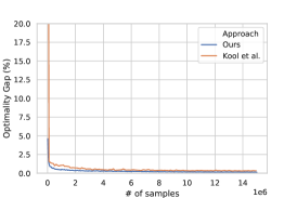
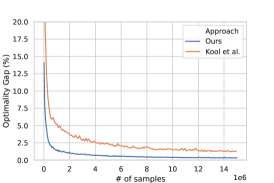
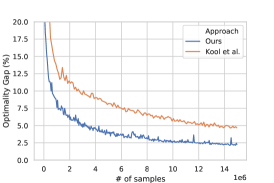
Figure 2 displays the validation optimality gap vs. number of training samples for our approach compared to Kool et al. (2019). For smaller instances (TSP20), both approaches find solutions within 1% of optimal after seeing less than 500,000 samples. More training samples are required to solve larger problem instances (TSP50 and TSP100). Our supervised training setup is more sample efficient compared to reinforcement learning as we train the model with complete information about the problem whereas RL training is guided by a sparse reward function.
It is important to note that each training graph is generated on the fly and is unique for RL. In contrast, our supervised approach randomly selects and repeats training graphs (and their groundtruth solutions) from a fixed set of one million instances.
Generalization to variable problem sizes
Generalization across TSP instances of various sizes is a highly desirable property for learning combinatorial problems. Size invariant generalization would allow us to scale up to very large TSP instances while training efficiently on smaller instances. In theory, since our model’s parameters are independent of the size of an instance , we can use a model trained on smaller graphs to solve arbitrarily large instances.
Table 2 presents the generalization performance of our approach and that of Kool et al. (2019) by evaluating the best performing models for fixed problem sizes on all other sizes. We observe drastic drops in performance for our non-autoregressive models, indicating very poor generalization capabilities. The representations learnt by the graph ConvNet are memorizing patterns for specific graph sizes and are unable to transfer to new graphs. In contrast, the autoregressive approach of Kool et al. (2019) displays a less drastic drop in generalization performance. In future work, we shall further explore generalization and transfer learning for large-scale combinatorial problems.
Training logs and additional results on model architecture are presented in Appendix C. Appendix D contains further discussion on supervised learning vs. reinforcement learning for combinatorial problems. Visualizations and qualitative analysis of solutions produced by our approach are available in Appendix E.
| Method/Model | TSP20 | TSP50 | TSP100 | ||||||
|---|---|---|---|---|---|---|---|---|---|
| Tour Len. | Opt. Gap. | Time | Tour Len. | Opt. Gap. | Time | Tour Len. | Opt. Gap. | Time | |
| Concorde | (1m) | (2m) | (3m) | ||||||
| TSP20 Model (Kool et al., 2019) | (5m) | (24m) | (1h) | ||||||
| TSP50 Model (Kool et al., 2019) | (5m) | (24m) | (1h) | ||||||
| TSP100 Model (Kool et al., 2019) | (5m) | (24m) | (1h) | ||||||
| TSP20 Model (Ours) | (20s) | (2m) | (10m) | ||||||
| TSP50 Model (Ours) | (20s) | (2m) | (10m) | ||||||
| TSP100 Model (Ours) | (20s) | (2m) | (10m) | ||||||
7 Conclusions
We introduce a novel learning-based approach for approximately solving the 2D Euclidean Travelling Salesman Problem using graph ConvNets and beam search. For fixed graph sizes, our framework outperforms all previous deep learning techniques in terms of solution quality, inference speed and sample efficiency due to better graph representation capacity, highly parallelized implementation and learning from optimal solutions. Future work shall explore incorporating transfer learning and reinforcement learning into our framework in order to generalize to large-scale problem instances and tackle previously un-encountered combinatorial problems beyond TSP.
Acknowledgement
The authors thank Victor Getty for helpful comments and discussions. XB is supported in part by NRF Fellowship NRFF2017-10.
References
- Angeniol et al. [1988] Bernard Angeniol, Gael De La Croix Vaubois, and Jean-Yves Le Texier. Self-organizing feature maps and the travelling salesman problem. Neural Networks, 1(4):289–293, 1988.
- Applegate et al. [2003] David Applegate, Robert Bixby, Vašek Chvátal, and William Cook. Implementing the dantzig-fulkerson-johnson algorithm for large traveling salesman problems. Mathematical programming, 97(1-2):91–153, 2003.
- Applegate et al. [2006] David L Applegate, Robert E Bixby, Vasek Chvatal, and William J Cook. The traveling salesman problem: a computational study. Princeton university press, 2006.
- Bahdanau et al. [2014] Dzmitry Bahdanau, Kyunghyun Cho, and Yoshua Bengio. Neural machine translation by jointly learning to align and translate. arXiv preprint arXiv:1409.0473, 2014.
- Bello et al. [2016] Irwan Bello, Hieu Pham, Quoc V Le, Mohammad Norouzi, and Samy Bengio. Neural combinatorial optimization with reinforcement learning. arXiv preprint arXiv:1611.09940, 2016.
- Bengio et al. [2018] Yoshua Bengio, Andrea Lodi, and Antoine Prouvost. Machine learning for combinatorial optimization: a methodological tour d’horizon. arXiv preprint arXiv:1811.06128, 2018.
- Bresson and Laurent [2017] Xavier Bresson and Thomas Laurent. Residual gated graph convnets. arXiv preprint arXiv:1711.07553, 2017.
- Bronstein et al. [2017] Michael M Bronstein, Joan Bruna, Yann LeCun, Arthur Szlam, and Pierre Vandergheynst. Geometric deep learning: going beyond euclidean data. IEEE Signal Processing Magazine, 34(4):18–42, 2017.
- Bruna et al. [2013] Joan Bruna, Wojciech Zaremba, Arthur Szlam, and Yann LeCun. Spectral networks and locally connected networks on graphs. arXiv preprint arXiv:1312.6203, 2013.
- Croes [1958] Georges A Croes. A method for solving traveling-salesman problems. Operations research, 6(6):791–812, 1958.
- Dai et al. [2016] Hanjun Dai, Bo Dai, and Le Song. Discriminative embeddings of latent variable models for structured data. In International conference on machine learning, pages 2702–2711, 2016.
- Dai et al. [2017] Hanjun Dai, Elias Khalil, Yuyu Zhang, Bistra Dilkina, and Le Song. Learning combinatorial optimization algorithms over graphs. In Advances in Neural Information Processing Systems, pages 6348–6358, 2017.
- Dantzig et al. [1954] George Dantzig, Ray Fulkerson, and Selmer Johnson. Solution of a large-scale traveling-salesman problem. Journal of the operations research society of America, 2(4):393–410, 1954.
- Defferrard et al. [2016] Michaël Defferrard, Xavier Bresson, and Pierre Vandergheynst. Convolutional neural networks on graphs with fast localized spectral filtering. In Advances in neural information processing systems, pages 3844–3852, 2016.
- Deudon et al. [2018] Michel Deudon, Pierre Cournut, Alexandre Lacoste, Yossiri Adulyasak, and Louis-Martin Rousseau. Learning heuristics for the tsp by policy gradient. In International Conference on the Integration of Constraint Programming, Artificial Intelligence, and Operations Research, pages 170–181. Springer, 2018.
- Fort [1988] JC Fort. Solving a combinatorial problem via self-organizing process: An application of the kohonen algorithm to the traveling salesman problem. Biological cybernetics, 59(1):33–40, 1988.
- Hamilton et al. [2017] Will Hamilton, Zhitao Ying, and Jure Leskovec. Inductive representation learning on large graphs. In Advances in Neural Information Processing Systems, pages 1024–1034, 2017.
- He et al. [2016] Kaiming He, Xiangyu Zhang, Shaoqing Ren, and Jian Sun. Deep residual learning for image recognition. In Proceedings of the IEEE conference on computer vision and pattern recognition, pages 770–778, 2016.
- Hopfield and Tank [1985] John J Hopfield and David W Tank. “neural” computation of decisions in optimization problems. Biological cybernetics, 52(3):141–152, 1985.
- Ioffe and Szegedy [2015] Sergey Ioffe and Christian Szegedy. Batch normalization: Accelerating deep network training by reducing internal covariate shift. arXiv preprint arXiv:1502.03167, 2015.
- Kaempfer and Wolf [2018] Yoav Kaempfer and Lior Wolf. Learning the multiple traveling salesmen problem with permutation invariant pooling networks. arXiv preprint arXiv:1803.09621, 2018.
- Kingma and Ba [2014] Diederik P Kingma and Jimmy Ba. Adam: A method for stochastic optimization. arXiv preprint arXiv:1412.6980, 2014.
- Kipf and Welling [2016] Thomas N Kipf and Max Welling. Semi-supervised classification with graph convolutional networks. arXiv preprint arXiv:1609.02907, 2016.
- Kool et al. [2019] Wouter Kool, Herke van Hoof, and Max Welling. Attention, learn to solve routing problems! In International Conference on Learning Representations, 2019. URL https://openreview.net/forum?id=ByxBFsRqYm.
- La Maire and Mladenov [2012] Bert FJ La Maire and Valeri M Mladenov. Comparison of neural networks for solving the travelling salesman problem. In 11th Symposium on Neural Network Applications in Electrical Engineering, pages 21–24. IEEE, 2012.
- Li et al. [2018] Zhuwen Li, Qifeng Chen, and Vladlen Koltun. Combinatorial optimization with graph convolutional networks and guided tree search. In Advances in Neural Information Processing Systems, pages 539–548, 2018.
- Marcheggiani and Titov [2017] Diego Marcheggiani and Ivan Titov. Encoding sentences with graph convolutional networks for semantic role labeling. arXiv preprint arXiv:1703.04826, 2017.
- Medress et al. [1977] Mark F. Medress, Franklin S Cooper, Jim W. Forgie, CC Green, Dennis H. Klatt, Michael H. O’Malley, Edward P Neuburg, Allen Newell, DR Reddy, B Ritea, et al. Speech understanding systems: Report of a steering committee. Artificial Intelligence, 9(3):307–316, 1977.
- Mittal et al. [2019] Akash Mittal, Anuj Dhawan, Sourav Medya, Sayan Ranu, and Ambuj Singh. Learning heuristics over large graphs via deep reinforcement learning. arXiv preprint arXiv:1903.03332, 2019.
- Mnih et al. [2013] Volodymyr Mnih, Koray Kavukcuoglu, David Silver, Alex Graves, Ioannis Antonoglou, Daan Wierstra, and Martin Riedmiller. Playing atari with deep reinforcement learning. arXiv preprint arXiv:1312.5602, 2013.
- Nazari et al. [2018] Mohammadreza Nazari, Afshin Oroojlooy, Lawrence Snyder, and Martin Takác. Reinforcement learning for solving the vehicle routing problem. In Advances in Neural Information Processing Systems, pages 9861–9871, 2018.
- Nowak et al. [2017] Alex Nowak, Soledad Villar, Afonso S Bandeira, and Joan Bruna. A note on learning algorithms for quadratic assignment with graph neural networks. arXiv preprint arXiv:1706.07450, 2017.
- Padberg and Rinaldi [1991] Manfred Padberg and Giovanni Rinaldi. A branch-and-cut algorithm for the resolution of large-scale symmetric traveling salesman problems. SIAM review, 33(1):60–100, 1991.
- Papadimitriou [1977] Christos H Papadimitriou. The euclidean travelling salesman problem is np-complete. Theoretical computer science, 4(3):237–244, 1977.
- Scarselli et al. [2009] Franco Scarselli, Marco Gori, Ah Chung Tsoi, Markus Hagenbuchner, and Gabriele Monfardini. The graph neural network model. IEEE Transactions on Neural Networks, 20(1):61–80, 2009.
- Smith [1999] Kate A Smith. Neural networks for combinatorial optimization: a review of more than a decade of research. INFORMS Journal on Computing, 11(1):15–34, 1999.
- Sukhbaatar et al. [2016] Sainbayar Sukhbaatar, Arthur Szlam, and Rob Fergus. Learning multiagent communication with backpropagation. In Advances in Neural Information Processing Systems, pages 2244–2252, 2016. URL https://openreview.net/forum?id=ByxBFsRqYm.
- Sutskever et al. [2014] Ilya Sutskever, Oriol Vinyals, and Quoc VV Le. Sequence to sequence learning with neural networks. In Advances in Neural Information Processing Systems, pages 3104–3112, 2014.
- Veličković et al. [2017] Petar Veličković, Guillem Cucurull, Arantxa Casanova, Adriana Romero, Pietro Lio, and Yoshua Bengio. Graph attention networks. arXiv preprint arXiv:1710.10903, 2017.
- Venkatakrishnan et al. [2018] Shaileshh Bojja Venkatakrishnan, Mohammad Alizadeh, and Pramod Viswanath. Graph2seq: Scalable learning dynamics for graphs. arXiv preprint arXiv:1802.04948, 2018.
- Vinyals et al. [2015] Oriol Vinyals, Meire Fortunato, and Navdeep Jaitly. Pointer networks. In Advances in Neural Information Processing Systems, pages 2692–2700, 2015.
- Williams [1992] Ronald J Williams. Simple statistical gradient-following algorithms for connectionist reinforcement learning. Machine learning, 8(3-4):229–256, 1992.
- Wu et al. [2016] Yonghui Wu, Mike Schuster, Zhifeng Chen, Quoc V Le, Mohammad Norouzi, Wolfgang Macherey, Maxim Krikun, Yuan Cao, Qin Gao, Klaus Macherey, et al. Google’s neural machine translation system: Bridging the gap between human and machine translation. arXiv preprint arXiv:1609.08144, 2016.
Appendix A Summary Statistics for Datasets
Summary statistics for various TSP datasets are presented in Table 3. We include TSP10 and TSP30 in addition to TSP20, TSP50 and TSP100. The approximate solver timings for Concorde are computed for a single-thread program on a 32-core CPU server under average load. Naturally, Concorde requires longer durations to find exact solutions as problem size increases. Generating datasets for problem sizes larger than 1,000 nodes would be impractical on a similar machine.
| Problem | Solver Time | Training set | Validation set | Test set | |||
|---|---|---|---|---|---|---|---|
| (approx.) | Tour Len. | Std. dev. | Tour Len. | Std. dev. | Tour Len. | Std. dev. | |
| TSP10 | ms | ||||||
| TSP20 | ms | ||||||
| TSP30 | ms | ||||||
| TSP50 | ms | ||||||
| TSP100 | ms | ||||||
Appendix B Graph Convolution Layer Details
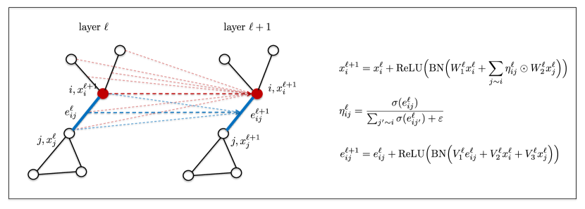
For the graph ConvNet described in Section 4.1, let denote the feature vector at layer associated with node . The activation at the next layer is obtained by applying a non-linear transformation to the feature vectors for all nodes in the neighborhood of node (defined by the graph structure). Thus, the most generic version of a feature vector at vertex in a graph ConvNet is:
| (8) |
where denotes the set of neighboring nodes centered at node . In other words, a graph ConvNet is defined by a mapping taking as input a vector (the feature vector of the center vertex) as well as an un-ordered set of vectors (the feature vectors of all neighboring vertices). The arbitrary choice of the mapping defines an instantiation of a class of graph neural networks such as Sukhbaatar et al. [2016], Kipf and Welling [2016], Hamilton et al. [2017].
For this work, we leverage the graph ConvNet architecture introduced in Bresson and Laurent [2017] by defining node features and edge features as follows:
| (9) | |||||
| (10) |
where , is the sigmoid function, is a small value, ReLU is the rectified linear unit, and BN stands for batch normalization. At the input layer, we have and .
Eq. (9) is similar to a learnable non-diffusion process on graphs where the diffusion time is the number of layers. As arbitrary graphs have no specific orientations (up, down, left, right), a diffusion process on graphs is consequently isotropic, making all neighbors equally important. However, this may not be true in general, e.g. a neighbor in the same community of a node shares different information than a neighbor in a separate community. We make the diffusion process anisotropic by point-wise multiplication operations with learneable normalized edge gates such as in [Marcheggiani and Titov, 2017]. Eq. (10) also represents a learnable non-diffusion process on graphs for the edge features. The network learns the best edge representations for encoding the information flow on the graph structure.
Additionally, we perform batch normalization [Ioffe and Szegedy, 2015] to enable fast training of deep architectures. Residual connections in Eq. (9) are essential to minimize the effect of the vanishing gradient problem on backpropagation [He et al., 2016]. Figure 3 illustrates the model.
Appendix C Additional Results
Training logs
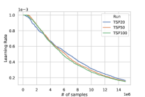
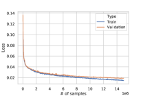
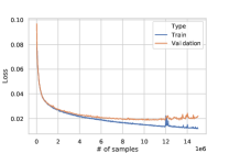
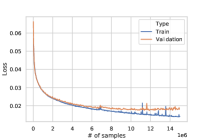
Figure 4 displays the learning rate and loss values vs. number of training samples for various runs. Decaying the learning rate to very small values allows the training loss to smoothly decrease. Loss curves for TSP50 and TSP100 show that models start overfitting to the training set after seeing approximately 4 million samples. However, as seen in Figure 2, the validation optimality gap does not get worse as models overfit to training data.
For faster training, TSP100 models were trained using four Nvidia 1080Ti GPUs. However, it is not essential to use a multi-GPU setup for training or evaluating our models: the same results can be attained with a single GPU by training longer.
Model capacity
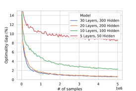
Figure 5a presents the validation optimality gap vs. number of training samples of TSP50 for various model capacities (defined as the number of graph convolution layers and hidden dimension). In general, we found that smaller models are able to learn smaller problem sizes at approximately the same closeness to optimality as larger models. Increasing model capacity leads to longer training time but is essential for scaling up to large problem sizes.
For consistency of analysis across problem sizes, our main results use models with the maximum capacity possible (30 layers, 300 hidden dimension) for our hardware setup (4 Nvidia 1080Ti GPUs) and the largest problem size (TSP100).
Beam width
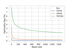
Figure 5b presents the validation optimality gap vs. beam width for various problem sizes. For smaller problem sizes, increasing beam width beyond 200 has a minor impact on performance. For TSP100, using large beam widths is essential for performance.
Reinforcement learning approaches such as Kool et al. [2019] sample 1,280 tours from the learnt policy (in < 1s on a single GPU for their model) and report the shortest among them as the final solution. For our main results, we use a beam width of 1,280 in order to directly compare with their approach. Due to the non-autoregressive nature of our approach, we can search using beam widths considerably larger than 1,280 within 1s on a single GPU.
Attention type
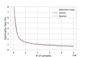
The classical softmax-based attention mechanism (such as that used in GAT) is a sparse attention where most of the importance is on the maximal value. In contrast, the sigmoid-based edge gating mechanism for our graph ConvNet (Eq. (4)) can be termed as a dense attention mechanism, where all saturated sigmoids lead to equal importance. We briefly experimented with both sparse and dense attention mechanisms for TSP and found dense attention to lead to marginally better performance and lesser GPU memory consumption. Figure 5c displays the validation optimality gap vs. number of training samples of TSP50 for both attention types (all other model hyperparameters are the same).
Appendix D Comments on Supervised Learning vs Reinforcement Learning
As noted in Bengio et al. [2018], the performance of supervised learning-based models for combinatorial optimization problems depends on the availability of a large set of optimal or high-quality solutions. Thus, two key issues arise when formulating these problems as supervised learning tasks: (1) we are restricted to learning well-studied problems for which optimal solvers or high-quality heuristic algorithms are available; and (2) we can only train on small-scale problem sizes as it is intractable to build datasets for large instances of NP-hard problems.
Although reinforcement learning is known to be more computationally expensive/less sample efficient than supervised learning, it does not require the generation of pairs of problem instances and solutions. As long as a problem can be formulated via a reward signal for making sequential decisions, a policy can be trained via RL. Hence, most recent work on learning-based approaches for TSP have used RL [Deudon et al., 2018, Kool et al., 2019]. Comparatively poor performance of SL methods [Vinyals et al., 2015, Nowak et al., 2017] have supported the argument in favour of reinforcement learning.
Unlike Vinyals et al. [2015] and Nowak et al. [2017], our approach uses deep graph ConvNets which are able to learn from a larger training set of optimal TSP solutions (one million instances). Our approach outperforms all other learning-based approaches in terms of both solution quality and sample efficiency. This result does not come as a surprise as SL techniques usually outperform RL techniques given sufficient amount of training data. However, the advantage of SL quickly diminishes for larger instances. Generating one million training samples for problem sizes beyond hundreds of nodes can become intractable in terms of computation and speed. The rapid increase in combinatorial complexity of TSP as problem size increases, termed as combinatorial explosion, makes it intractable to scale our approach to large TSPs.
Thus, incorporating RL to tackle arbitrary problem sizes is the next natural development for our approach: Future work shall explore learning a policy network by graph ConvNet, optimizing the tour length and applying beam search without optimal solutions. Supervised training on small instances and transfer learning by fine-tuning model parameters on large instances using RL is an attractive approach for scaling up to realistic sizes beyond hundreds of nodes.
Appendix E Solution Visualizations
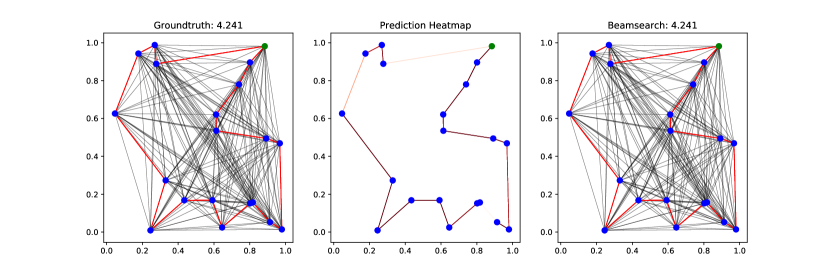
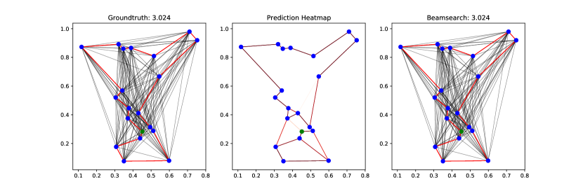
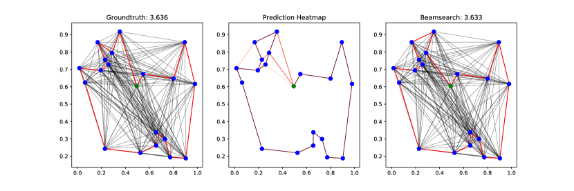
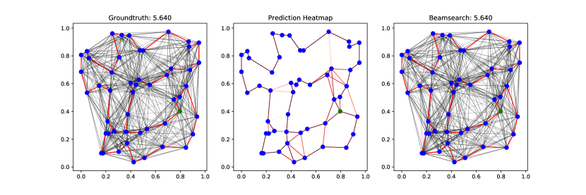
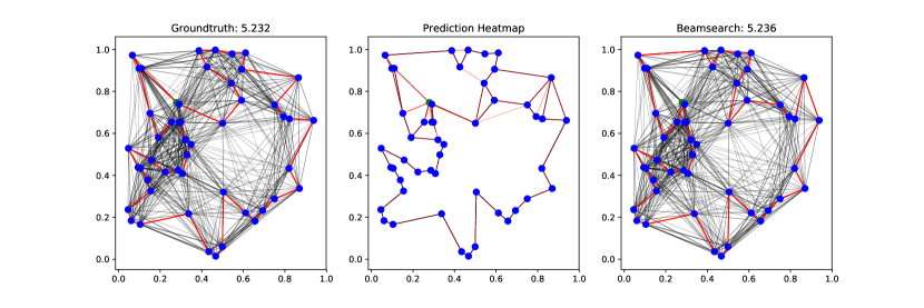
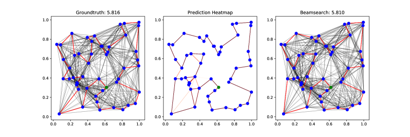
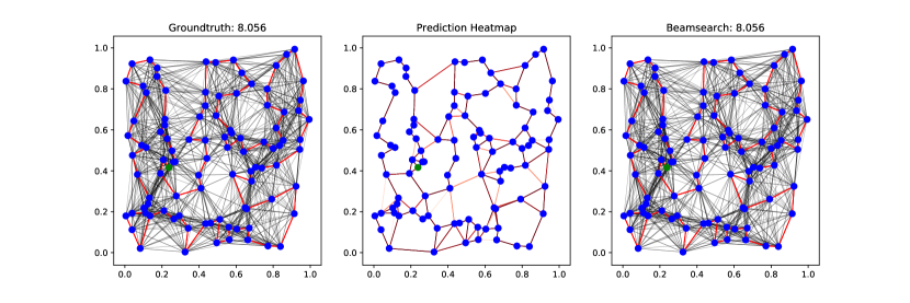
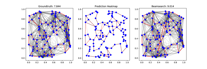
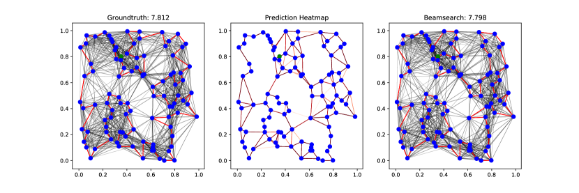
Figures 6, 7 and 8 display prediction visualizations for samples from test sets of various problem instances. In each figure, the first panel shows the input -nearest neighbor graph and the groundtruth TSP tour. The second panel represents the probabilistic heat-map output of the graph ConvNet model. The final panel shows the predicted TSP tour after a beam search procedure on the heat-map.
For small instances where the nodes are evenly distributed, the model is able to confidently identify most of the tour edges in the heat-map, resulting in greedy search being able to find close to optimal tours. As instance size increases, the prediction heat-map reflects the combinatorial explosion in TSP and beam search is essential for finding the optimal tour.
