Conversational Contextual Bandit: Algorithm and Application

Xiaoying Zhang CSE, The Chinese University of Hong Kong xyzhang@cse.cuhk.edu.hk Hong Xie College of Computer Science, Chongqing University xiehong2018@cqu.edu.cn Hang Li AI Lab, Bytedance lihang.lh@bytedance.com  and  John C.S. Lui CSE, The Chinese University of Hong Kong cslui@cse.cuhk.edu.hk
(2020)
Abstract.

Contextual bandit algorithms provide principled online learning solutions to balance the exploitation-exploration trade-off in various applications such as recommender systems. However, the learning speed of the traditional contextual bandit algorithms is often slow due to the need for extensive exploration. This poses a critical issue in applications like recommender systems, since users may need to provide feedbacks on a lot of uninterested items. To accelerate the learning speed, we generalize contextual bandit to conversational contextual bandit. Conversational contextual bandit leverages not only behavioral feedbacks on arms (e.g., articles in news recommendation), but also occasional conversational feedbacks on key-terms from the user. Here, a key-term can relate to a subset of arms, for example, a category of articles in news recommendation. We then design the Conversational UCB algorithm (ConUCB) to address two challenges in conversational contextual bandit: (1) which key-terms to select to conduct conversation, (2) how to leverage conversational feedbacks to accelerate the speed of bandit learning. We theoretically prove that ConUCB can achieve a smaller regret upper bound than the traditional contextual bandit algorithm LinUCB, which implies a faster learning speed. Experiments on synthetic data, as well as real datasets from Yelp and Toutiao, demonstrate the efficacy of the ConUCB algorithm.

journalyear: 2020copyright: iw3c2w3conference: Proceedings of The Web Conference 2020; April 20–24, 2020; Taipei, Taiwanbooktitle: Proceedings of The Web Conference 2020 (WWW ’20), April 20–24, 2020, Taipei, Taiwandoi: 10.1145/3366423.3380148isbn: 978-1-4503-7023-3/20/04copyright: none

1. Introduction

Contextual bandit serves as an invaluable tool for enhancing performance of a system through learning from interactions with the user while making trade-off between exploitation and exploration (Abbasi-Yadkori et al., 2011; Li et al., 2010, 2016; Wang et al., 2016). The contextual bandit algorithms have been applied to recommender systems, for instance, to adaptively learn users’ preference on items. In this application, the items are taken as the arms in contextual bandit, and the contextual vector of each arm/item contains the observed information about the user and the item at the time. The recommender system equipped with a contextual bandit algorithm sequentially recommends items to the user. The user provides a feedback (e.g., click) on the recommended item each round, which is viewed as a reward. The goal of the contextual bandit algorithm is to learn an item recommendation (arm selection) strategy to optimize the user’s feedbacks in the long run (cumulative rewards), via utilizing the information of the user and items (contextual vectors) as well as the user’s feedbacks (rewards). In general, the algorithm needs to make a trade-off between exploitation (i.e., leveraging the user’s preference already known) and exploration (i.e., revealing the user’s preference still unknown).

One shortcoming of the traditional contextual bandit algorithms (Abbasi-Yadkori et al., 2011; Li et al., 2010, 2016; Wang et al., 2016) lies in their slow learning speed. This is because they need to perform extensive exploration in order to collect sufficient feedbacks. For applications like recommender systems, it poses a critical issue, because it means that the user needs to provide feedbacks on a large number of items which she is not interested in.

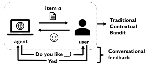
Recently, a number of researchers propose the construction of conversational recommender systems that leverage conversations to elicit users’ preference for better recommendation (e.g.,  (Christakopoulou et al., 2016, 2018)). Inspired by this, we consider a novel contextual bandit setting in this paper, i.e., conversational contextual bandit, which incorporates a conversation mechanism into the traditional contextual bandit algorithm (as shown in Figure 1), for accelerating bandit learning.
Refer to caption
Figure 1. Conversational contextual bandit. The part in dashed box corresponds to traditional contextual bandit.

To illustrate the benefits of the conversation mechanism, let us consider the news recommendation scenario with conversational contextual bandit. In this scenario, the agent/system also occasionally asks questions with regard to the user’s preference on key-terms. For example, asking about the user’s preference on a category: “Are you interested in news about basketball?”, or asking about the user’s preference on an entity: “Do you like to read news related to LeBron James?”. There are two reasons why conversations can improve the learning speed. First, the key-terms like “basketball” and “LeBron James” can be associated with a large number of articles. Thus feedback on one key-term may contain a large amount of information about the user’s preference. Traditional contextual bandit algorithms  (Abbasi-Yadkori et al., 2011; Li et al., 2010, 2016; Wang et al., 2016) may spend many interactions to collect the information, because many articles, that are related to the same key-term, may have different contextual vectors. For example, the contextual vector of an article about NBA games may be far from that of an article about basketball shoes, though they are all related to the key-term “basketball”. Second, collecting explicit feedback from the user can help the system to capture the user’s true preference faster. For example, the fact that the user reads an article of NBA game with “LeBron James” may be because she concerns about the result of the game or because she is a fan of LeBron James. To figure out which is more likely, instead of recommending articles related to each possibility, a more convenient way is to directly ask the user “Do you want to read more news about LeBron James?”.

In this paper, the agent conducts conversations by asking the user’s preference on key-terms. Here, a key-term is related to a subset of arms, and can be a category or topic. We assume that there exists a bipartite graph of key-terms and arms in which the relations between key-terms and arms are represented. The agent occasionally selects key-terms and asks the user about her preference over the key-terms. Then, the user shows her feedbacks to the agent, for example, indicating whether she is interested in the key-terms. The preference over the key-term is then “propagated” to the related arms, and is leveraged by the algorithm to select arms and update the bandit model. To the best of our knowledge, this is the first time such an approach is proposed.

There are two main challenges for conversational contextual bandit: (1) which key-terms to select for querying, (2) how to leverage conversational feedbacks to build a more accurate bandit model. We design the Conversational UCB algorithm (ConUCB) to address these challenges.

The ConUCB algorithm, as a generalization of the LinUCB algorithm (Abbasi-Yadkori et al., 2011), repeatedly conducts learning as follows: (1) If conversation is allowed at the round, given the current context and historical interactions on arms and key-terms, ConUCB selects the key-terms that reduce the learning error most, and enquires the user’s preference over the key-terms; (2) It selects the arm with the largest upper confidence bound derived from both arm-level and key-term-level feedbacks, and receives a reward. The interaction record will then be leveraged for key-term selection. Theoretical analysis shows that ConUCB achieves a lower cumulative regret upper bound than the standard contextual bandit algorithm LinUCB. Note that a smaller regret upper bound means that the agent learns parameters more accurately within the same number of iterations, i.e., the speed of bandit learning is accelerated. Experimental results on a synthetic dataset, as well as real datasets from Yelp and Toutiao (the largest news recommendation platform in China) show that the ConUCB algorithm significantly outperforms the baseline algorithms including LinUCB. Note that the basic mechanism of adding conversation into bandit algorithms to speed up learning is generic. We demonstrate that ConUCB can be easily extended to other contextual bandit algorithms such as hLinUCB (Wang et al., 2016).

In summary, our contributions are as follows:

  • We formulate the new conversational contextual bandit problem to improve the learning speed (Section 2).

  • We design the ConUCB algorithm by generalizing LinUCB for conversational contextual bandit and theoretically prove that it can achieve a smaller regret upper bound than the conventional contextual bandit algorithm LinUCB, i.e., the learning speed is improved (Section 3).

  • We empirically verify the improvement of ConUCB in learning speed using both a synthetic dataset and real-world datasets (Section 4 & 5).

  • We also extend ConUCB by adding the conversation mechanism into hLinUCB (Section 6).

2. Problem Formulation

We first introduce traditional contextual bandit and then we generalize it to obtain conversational contextual bandit. Without loss of generality, we take the UCB algorithm as an example algorithm of contextual bandit.

2.1. Contextual Bandit

In contextual bandit, the agent learns to maximize the cumulative reward in T+𝑇subscriptT\in\mathbb{N}_{+} rounds through interaction with the user.

Consider a finite set of N𝑁N arms denoted by 𝒜𝒜\mathcal{A}. At each round t=1,,T𝑡1𝑇t=1,\ldots,T, the agent is given a subset of arms 𝒜t𝒜subscript𝒜𝑡𝒜\mathcal{A}_{t}\subseteq\mathcal{A}, and each arm a𝒜t𝑎subscript𝒜𝑡a\in\mathcal{A}_{t} is associated with a d𝑑d-dimensional contextual vector 𝒙a,tdsubscript𝒙𝑎𝑡superscript𝑑\bm{x}_{a,t}\in\mathbb{R}^{d}, which describes the observable information of arm a𝑎a and the user at round t𝑡t. The agent chooses an arm atsubscript𝑎𝑡a_{t} on the basis of its contextual vector 𝒙at,tsubscript𝒙subscript𝑎𝑡𝑡\bm{x}_{a_{t},t}, shows it to the user, and receives a reward rat,tsubscript𝑟subscript𝑎𝑡𝑡r_{a_{t},t}\in\mathcal{R}. For example, ={0,1}01\mathcal{R}=\{0,1\} represents a binary reward, and =\mathcal{R}=\mathbb{R} represents a continuous reward. The reward rat,tsubscript𝑟subscript𝑎𝑡𝑡r_{a_{t},t} is a function of the contextual vector 𝒙at,tsubscript𝒙subscript𝑎𝑡𝑡\bm{x}_{a_{t},t} and the parameter vector 𝜽𝜽\bm{\theta}. The parameter vector 𝜽𝜽\bm{\theta} represents the user’s preference and is what the agent wants to learn. At each round t𝑡t, the agent takes the selected arms a1,,at1subscript𝑎1subscript𝑎𝑡1a_{1},\ldots,a_{t-1} and received rewards ra1,1,,rat1,t1subscript𝑟subscript𝑎11subscript𝑟subscript𝑎𝑡1𝑡1r_{a_{1},1},\ldots,r_{a_{t-1},t-1} at the previous rounds as input, to estimate the reward and select the arm at𝒜tsubscript𝑎𝑡subscript𝒜𝑡a_{t}\in\mathcal{A}_{t}.

The goal of the agent is to maximize the expected cumulative rewards. Let t=1T𝔼[rat,t]subscriptsuperscript𝑇𝑡1𝔼delimited-[]subscript𝑟subscriptsuperscript𝑎𝑡𝑡\sum^{T}_{t=1}\mathbb{E}[r_{a^{\ast}_{t},t}] denote the maximum expected cumulative rewards in T𝑇T rounds, where at𝒜tsubscriptsuperscript𝑎𝑡subscript𝒜𝑡a^{\ast}_{t}\in\mathcal{A}_{t} is the optimal arm at round t𝑡t, i.e., 𝔼[rat,t]𝔼[ra,t],a𝒜tformulae-sequence𝔼delimited-[]subscript𝑟subscriptsuperscript𝑎𝑡𝑡𝔼delimited-[]subscript𝑟𝑎𝑡for-all𝑎subscript𝒜𝑡\mathbb{E}[r_{a^{\ast}_{t},t}]\geq\mathbb{E}[r_{a,t}],\forall a\in\mathcal{A}_{t}. The goal of contextual bandit learning is formally defined as minimization of the cumulative regret in T𝑇T rounds:

(1) R(T)t=1T(𝔼[rat,t]𝔼[rat,t]).𝑅𝑇superscriptsubscript𝑡1𝑇𝔼delimited-[]subscript𝑟subscriptsuperscript𝑎𝑡𝑡𝔼delimited-[]subscript𝑟subscript𝑎𝑡𝑡\textstyle R(T)\triangleq\sum\nolimits_{t=1}^{T}\left(\mathbb{E}[r_{a^{*}_{t},t}]-\mathbb{E}[r_{a_{t},t}]\right).

The agent needs to make a trade-off between exploitation (i.e., choose the best arm estimated from received feedbacks) and exploration (i.e., seek feedbacks from arms that the agent is unsure about).

Let us consider the UCB (Upper Confidence Bound) algorithm. The agent selects the arm atsubscript𝑎𝑡a_{t} at each round t𝑡t as follows:

at=argmaxa𝒜tRa,t+Ca,t,subscript𝑎𝑡subscript𝑎subscript𝒜𝑡subscript𝑅𝑎𝑡subscript𝐶𝑎𝑡\textstyle a_{t}=\arg\max_{a\in\mathcal{A}_{t}}R_{a,t}+C_{a,t},

where Ra,tsubscript𝑅𝑎𝑡R_{a,t} and Ca,tsubscript𝐶𝑎𝑡C_{a,t} are the estimated reward and confidence interval of arm a𝑎a at round t𝑡t respectively. The confidence interval Ca,tsubscript𝐶𝑎𝑡C_{a,t} measures the uncertainty of reward estimation of arm a𝑎a at round t𝑡t. In the LinUCB algorithm (Abbasi-Yadkori et al., 2011), the reward function is defined as a linear function,

(2) rat,t=𝒙at,tT𝜽+ϵt,subscript𝑟subscript𝑎𝑡𝑡superscriptsubscript𝒙subscript𝑎𝑡𝑡𝑇𝜽subscriptitalic-ϵ𝑡\textstyle r_{a_{t},t}=\bm{x}_{a_{t},t}^{T}\bm{\theta}+\epsilon_{t},

where 𝜽𝜽\bm{\theta} is a d𝑑d-dimensional parameter vector, ϵtsubscriptitalic-ϵ𝑡\epsilon_{t} is a random variable representing the random noise. One can also generalize LinUCB by utilizing non-linear reward (Filippi et al., 2010) or hidden features (Wang et al., 2016).

In news recommendation with contextual bandit, for example, the agent is the recommender system, each arm a𝑎a is an article, the contextual vector 𝒙a,tsubscript𝒙𝑎𝑡\bm{x}_{a,t} denotes the observable information of the user and the article a𝑎a at round t𝑡t, and the reward ra,tsubscript𝑟𝑎𝑡r_{a,t} is whether the user clicks article a𝑎a at round t𝑡t. The parameter vector 𝜽𝜽\bm{\theta} represents the user’s preference on articles. The goal of the system is to maximize the cumulative click-through rate (CTR) of the user.

2.2. Conversational Contextual Bandit

In conversational contextual bandit, the agent still learns to maximize the cumulative reward in T𝑇T rounds through interacting with the user. In addition to collecting feedbacks on selected arms, the agent also occasionally conducts conversations with the user and learns from conversational feedbacks.

We consider that the agent conducts conversations by asking the user’s preference on key-terms, where a key-term is related to a subset of arms, and can be a category, topic, etc. For example, in news recommendation, a key-term can be a keyword, a key-phrase, or a combination of multiple single keywords, extracted from articles. The agent may ask the user “Are you interested in news about basketball?” The user shows her answer to the question.

Problem formulation. Consider a finite set of N+𝑁subscriptN\in\mathbb{N}_{+} arms denoted by 𝒜𝒜\mathcal{A} and a finite set of K+𝐾subscriptK\in\mathbb{N}_{+} key-terms denoted by 𝒦𝒦\mathcal{K}. The relationships between the arms and the key-terms are characterized by a weighted bipartite graph (𝒜,𝒦,𝑾)𝒜𝒦𝑾(\mathcal{A},\mathcal{K},\bm{W}), whose nodes are divided into two sets 𝒜𝒜\mathcal{A} and 𝒦𝒦\mathcal{K}, and weighted edges are represented by the matrix 𝑾[wa,k]𝑾delimited-[]subscript𝑤𝑎𝑘\bm{W}\triangleq[w_{a,k}]. Here wa,ksubscript𝑤𝑎𝑘w_{a,k} represents the relationship between arm a𝑎a and key-term k𝑘k. Without loss of generality, we normalize the total weights associated with each arm to be 1, i.e., kwa,k=1subscript𝑘subscript𝑤𝑎𝑘1\sum_{k}w_{a,k}=1.

We also introduce a function b(t)𝑏𝑡b(t) to model the frequency of conversations. Note that b(t)𝑏𝑡b(t) determines: (1) whether to converse at round t𝑡t; (2) the number of conversations until round t𝑡t. To make it clearer, consider a function q(t)𝑞𝑡q(t):

q(t)={1,b(t)b(t1)>0,0,otherwise.𝑞𝑡cases1𝑏𝑡𝑏𝑡100otherwise\textstyle q(t)=\left\{\begin{array}[]{cl}1,&b(t)-b(t-1)>0,\\ 0,&\mbox{otherwise}.\end{array}\right.\vspace{-2mm}

If q(t)=1𝑞𝑡1q(t)=1, then the agent conducts conversation with the user at round t𝑡t; if q(t)=0𝑞𝑡0q(t)=0, then it does not. The agent conducts b(t)𝑏𝑡b(t) conversations up to round t𝑡t. For example, if b(t)=ktm,m1,k1formulae-sequence𝑏𝑡𝑘𝑡𝑚formulae-sequence𝑚1𝑘1b(t)=k\lfloor\frac{t}{m}\rfloor,m\geq 1,k\geq 1, then the agent makes k𝑘k conversations in every m𝑚m rounds. If b(t)=log(t)𝑏𝑡𝑡b(t)=\lfloor\log(t)\rfloor, then the agent makes a conversation with a frequency represented by the logarithmic function of t𝑡t. If b(t)0𝑏𝑡0b(t)\equiv 0, then there is no conversation between the agent and the user. Moreover, we assume that key-term-level conversations should be less frequent than arm-level interactions, i.e., b(t)t,t𝑏𝑡𝑡for-all𝑡b(t)\leq t,\forall t, in consideration of users’ experience.

At each round t=1,,T𝑡1𝑇t=1,\ldots,T, the agent is given a subset of arms 𝒜t𝒜subscript𝒜𝑡𝒜\mathcal{A}_{t}\subseteq\mathcal{A}, and each arm a𝒜t𝑎subscript𝒜𝑡a\in\mathcal{A}_{t} is specified by a contextual vector 𝒙a,tdsubscript𝒙𝑎𝑡superscript𝑑\bm{x}_{a,t}\in\mathbb{R}^{d}. Without loss of generality, we normalize the contextual vector such that 𝒙a,t2=1subscriptnormsubscript𝒙𝑎𝑡21\|\bm{x}_{a,t}\|_{2}=1. Based on the arm-level feedbacks and conversational feedbacks received in the previous t1𝑡1t-1 rounds,

  • If q(t)=1𝑞𝑡1q(t)=1, the agent conducts b(t)b(t1)𝑏𝑡𝑏𝑡1\lfloor b(t)-b(t-1)\rfloor conversations with the user. In each conversation, the agent asks the user’s preference on one selected key-term k𝒦𝑘𝒦k\in\mathcal{K}, and gets the user’s feedback r~k,tsubscript~𝑟𝑘𝑡\tilde{r}_{k,t}. For example, r~k,tsubscript~𝑟𝑘𝑡\tilde{r}_{k,t} can be binary {0,1}01\{0,1\}, where 00 and 111 stand for negative and positive feedback respectively.

  • The agent chooses an arm at𝒜tsubscript𝑎𝑡subscript𝒜𝑡a_{t}\in\mathcal{A}_{t}, presents it to the user, and receives the reward of arm atsubscript𝑎𝑡a_{t}, denoted by rat,tsubscript𝑟subscript𝑎𝑡𝑡r_{a_{t},t}.

The agent tries to speed up the learning process by leveraging conversational feedbacks. The problems in conversational contextual bandit are to find (a) an effective arm selection strategy and (b) an effective key-term selection strategy, so that after T𝑇T rounds of arm-level interactions and b(T)𝑏𝑇b(T) times of conversations, the cumulative regret in Eq. (10) is significantly reduced.

General algorithm of conversational UCB (ConUCB). Algorithm 1 outlines the general algorithm of ConUCB, which will be described in detail in Section 3. One can see that when no conversation is performed between the agent and the user, conversational contextual bandit degenerates to standard contextual bandit. In ConUCB, the agent selects an arm with the following strategy

(3) at=argmaxa𝒜tR~a,t+Ca,t,subscript𝑎𝑡subscript𝑎subscript𝒜𝑡subscript~𝑅𝑎𝑡subscript𝐶𝑎𝑡\textstyle a_{t}=\arg\max\nolimits_{a\in\mathcal{A}_{t}}\tilde{R}_{a,t}+C_{a,t},

where R~a,tsubscript~𝑅𝑎𝑡\tilde{R}_{a,t} and Ca,tsubscript𝐶𝑎𝑡C_{a,t} are the estimated reward and the confidence interval of arm a𝑎a at round t𝑡t respectively. As will be shown in Section 3 later, R~a,tsubscript~𝑅𝑎𝑡\tilde{R}_{a,t} is inferred from both arm-level and key-term-level feedbacks, and Ca,tsubscript𝐶𝑎𝑡C_{a,t} contains both arm-level and key-term-level confidence interval.

Input: arms 𝒜𝒜\mathcal{A}, key-terms 𝒦𝒦\mathcal{K}, graph (𝒜,𝒦,𝑾)𝒜𝒦𝑾(\mathcal{A},\mathcal{K},\bm{W}), b(t)𝑏𝑡b(t).
1 for  t=1,,T𝑡1𝑇t=1,\ldots,T do
2       observe contextual vector 𝒙a,tsubscript𝒙𝑎𝑡\bm{x}_{a,t} of each arm a𝒜t𝑎subscript𝒜𝑡a\in\mathcal{A}_{t};
3       If conversation is allowed at round t𝑡t, i.e., q(t)=1𝑞𝑡1q(t)=1, select key-terms to conduct conversations and receive conversational feedbacks {r~k,t}subscript~𝑟𝑘𝑡\{\tilde{r}_{k,t}\};
4       select an arm at=argmaxa𝒜tR~a,t+Ca,tsubscript𝑎𝑡subscript𝑎subscript𝒜𝑡subscript~𝑅𝑎𝑡subscript𝐶𝑎𝑡a_{t}=\arg\max_{a\in\mathcal{A}_{t}}\tilde{R}_{a,t}+C_{a,t} ;
5       receive a reward rat,tsubscript𝑟subscript𝑎𝑡𝑡r_{a_{t},t};
6       update model ;
7      
Algorithm 1 General algorithm of ConUCB

In ConUCB, the user’s feedback on key-term k𝑘k, i.e., r~k,tsubscript~𝑟𝑘𝑡\tilde{r}_{k,t}, is estimated from the user’s feedbacks on related arms, i.e.,

(4) 𝔼[r~k,t]=a𝒜wa,ka𝒜wa,k𝔼[ra,t],k𝒦.formulae-sequence𝔼delimited-[]subscript~𝑟𝑘𝑡subscript𝑎𝒜subscript𝑤𝑎𝑘subscriptsuperscript𝑎𝒜subscript𝑤superscript𝑎𝑘𝔼delimited-[]subscript𝑟𝑎𝑡𝑘𝒦\textstyle\mathbb{E}[\tilde{r}_{k,t}]=\sum\nolimits_{a\in\mathcal{A}}\frac{w_{a,k}}{\sum_{a^{\prime}\in\mathcal{A}}w_{a^{\prime},k}}\mathbb{E}[r_{a,t}],\quad k\in\mathcal{K}.

Equivalently, r~k,t=a𝒜wa,ka𝒜wa,k𝔼[ra,t]+ϵ~k,tsubscript~𝑟𝑘𝑡subscript𝑎𝒜subscript𝑤𝑎𝑘subscriptsuperscript𝑎𝒜subscript𝑤superscript𝑎𝑘𝔼delimited-[]subscript𝑟𝑎𝑡subscript~italic-ϵ𝑘𝑡\tilde{r}_{k,t}=\sum_{a\in\mathcal{A}}\frac{w_{a,k}}{\sum_{a^{\prime}\in\mathcal{A}}w_{a^{\prime},k}}\mathbb{E}[r_{a,t}]+\tilde{\epsilon}_{k,t}, where ϵ~k,tsubscript~italic-ϵ𝑘𝑡\tilde{\epsilon}_{k,t} is a random variable representing the random noise in reward. When both the conversational feedback r~k,tsubscript~𝑟𝑘𝑡\tilde{r}_{k,t} and arm-level feedback ra,tsubscript𝑟𝑎𝑡r_{a,t} are binary, Eq. (4) has a probabilistic interpretation. Specifically, for binary feedback c{0,1}𝑐01c\in\{0,1\}, we have

(5) (c|k,t)=a𝒜(a|k)(c|a,t),conditional𝑐𝑘𝑡subscript𝑎𝒜conditional𝑎𝑘conditional𝑐𝑎𝑡\textstyle\mathbb{P}(c|k,t)=\sum\nolimits_{a\in\mathcal{A}}\mathbb{P}(a|k)\mathbb{P}(c|a,t),

where (c=1|k,t)𝑐conditional1𝑘𝑡\mathbb{P}(c=1|k,t) and (c=0|k,t)𝑐conditional0𝑘𝑡\mathbb{P}(c=0|k,t) represent the probabilities that the user gives a positive and negative feedback to the question with key-term k𝑘k at round t𝑡t respectively; (c=1|a,t)𝑐conditional1𝑎𝑡\mathbb{P}(c=1|a,t) and (c=0|a,t)𝑐conditional0𝑎𝑡\mathbb{P}(c=0|a,t) denote the probabilities that the user likes and dislikes arm a𝑎a at round t𝑡t respectively. Thus, if we take 𝔼[ra,t]=(c=1|a,t)𝔼delimited-[]subscript𝑟𝑎𝑡𝑐conditional1𝑎𝑡\mathbb{E}[r_{a,t}]=\mathbb{P}(c=1|a,t), 𝔼[r~k,t]=(c=1|k,t)𝔼delimited-[]subscript~𝑟𝑘𝑡𝑐conditional1𝑘𝑡\mathbb{E}[\tilde{r}_{k,t}]=\mathbb{P}(c{=}1|k,t), and (a|k)=wa,ka𝒜wa,kconditional𝑎𝑘subscript𝑤𝑎𝑘subscriptsuperscript𝑎𝒜subscript𝑤superscript𝑎𝑘\mathbb{P}(a|k){=}\frac{w_{a,k}}{\sum_{a^{\prime}\in\mathcal{A}}w_{a^{\prime},k}}, we obtain Eq. (5).

3. Algorithm & Theoretical Analysis

In this section, we present the details of ConUCB by providing specific solutions to the two problems in Algorithm 1: (1) how to select key-terms to conduct conversation (Line 3), (2) how to select an arm, i.e., calculate R~a,tsubscript~𝑅𝑎𝑡\tilde{R}_{a,t} and Ca,tsubscript𝐶𝑎𝑡C_{a,t} (Line 4). ConUCB is a generalization of LinUCB (Abbasi-Yadkori et al., 2011) in the sense that the arm-level reward function is the same as that of LinUCB in Eq. (2). We theoretically analyze the upper bound of its cumulative regret and discuss the impact of conversational feedbacks. We note that ConUCB has a generic mechanism of selecting key-terms and leveraging feedbacks on key-terms to speed up learning, which can be easily incorporated into a variety of contextual bandit algorithms such as CoFineUCB (Yue et al., 2012), hLinUCB (Wang et al., 2016). In Section 6, we explain how to apply the same technique to the hLinUCB algorithm.

3.1. ConUCB Algorithm

The ConUCB algorithm is described in Algo. 2. It contains a key-term selection module to select key-terms (line 2-11) and an arm-selection module to select arms (line 12-15). The two modules collaborate with each other as follows:

  • If conversation is allowed at round t𝑡t, given the current context and interaction histories on both arms and key-terms, the key-term selection module repeatedly selects the key-term that minimizes the regret and asks the user’s preference over it (line 5). Then the newly estimated key-term-level parameter vector (𝜽~tsubscript~𝜽𝑡\tilde{\bm{\theta}}_{t}) is passed to the arm-selection module.

  • Under the guidance of 𝜽~tsubscript~𝜽𝑡\tilde{\bm{\theta}}_{t} and rewards received up to round t𝑡t, the arm-selection module recommends an arm to the user, and receives a reward (line 12-15). The interaction record will then be leveraged by the key-term selection module.

3.1.1. Arm selection.

At round t𝑡t, ConUCB first estimates the user’s preference at the key-term level, denoted as 𝜽~tsubscript~𝜽𝑡\tilde{\bm{\theta}}_{t}, by

𝜽~t=argmin𝜽~τ=1tk𝒦τ(a𝒜wa,k𝜽~T𝒙a,τa𝒜wa,kr~k,τ)2+λ~𝜽~22,subscriptbold-~𝜽𝑡subscriptbold-~𝜽subscriptsuperscript𝑡𝜏1subscript𝑘subscript𝒦𝜏superscriptsubscript𝑎𝒜subscript𝑤𝑎𝑘superscriptbold-~𝜽𝑇subscript𝒙𝑎𝜏subscript𝑎𝒜subscript𝑤𝑎𝑘subscript~𝑟𝑘𝜏2~𝜆superscriptsubscriptnormbold-~𝜽22\displaystyle\textstyle\bm{\tilde{\theta}}_{t}{=}\arg\min_{\bm{\tilde{\theta}}}\sum^{t}_{\tau=1}\sum_{k\in\mathcal{K}_{\tau}}\left(\frac{\sum_{a\in\mathcal{A}}w_{a,k}\bm{\tilde{\theta}}^{T}\bm{x}_{a,\tau}}{\sum_{a\in\mathcal{A}}w_{a,k}}{-}\tilde{r}_{k,\tau}\right)^{2}{+}\tilde{\lambda}\|\bm{\tilde{\theta}}\|_{2}^{2},

where 𝒦τsubscript𝒦𝜏\mathcal{K}_{\tau} denotes the set of key-terms queried at round τ𝜏\tau. We set 𝒦τ=subscript𝒦𝜏\mathcal{K}_{\tau}=\emptyset if no key-term is queried, and we let 𝒦τsubscript𝒦𝜏\mathcal{K}_{\tau} contain duplicated elements if querying a key-term multiple times at the round. The coefficient λ~~𝜆\tilde{\lambda}\in\mathbb{R} controls regularization. Then 𝜽~tsubscriptbold-~𝜽𝑡\bm{\tilde{\theta}}_{t} is used to guide the learning of the arm-level parameter vector at round t𝑡t:

𝜽𝒕=argmin𝜽λτ=1t1(𝜽T𝒙aτ,τraτ,τ)2+(1λ)𝜽𝜽~t22.subscript𝜽𝒕subscript𝜽𝜆superscriptsubscript𝜏1𝑡1superscriptsuperscript𝜽𝑇subscript𝒙subscript𝑎𝜏𝜏subscript𝑟subscript𝑎𝜏𝜏21𝜆superscriptsubscriptnorm𝜽subscriptbold-~𝜽𝑡22\displaystyle\textstyle\bm{\theta_{t}}{=}\arg\min_{\bm{\theta}}\ \lambda\sum_{\tau=1}^{t-1}(\bm{\theta}^{T}\bm{x}_{a_{\tau},\tau}{-}r_{a_{\tau},\tau})^{2}{+}(1{-}\lambda)\|\bm{\theta}-\bm{\tilde{\theta}}_{t}\|_{2}^{2}.

where λ[0,1]𝜆01\lambda{\in}[0,1] balances learning from rewards at arm-level and learning from feedbacks at key-term-level (i.e., 𝜽~tsubscriptbold-~𝜽𝑡\bm{\tilde{\theta}}_{t}). Both optimization problems have closed-form solutions, 𝜽~t=𝑴~t1𝒃~tsubscriptbold-~𝜽𝑡superscriptsubscriptbold-~𝑴𝑡1subscriptbold-~𝒃𝑡\bm{\tilde{\theta}}_{t}=\bm{\tilde{M}}_{t}^{-1}\bm{\tilde{b}}_{t} and 𝜽t=𝑴t1(𝒃t+(1λ)𝜽~t)subscript𝜽𝑡superscriptsubscript𝑴𝑡1subscript𝒃𝑡1𝜆subscriptbold-~𝜽𝑡\bm{\theta}_{t}=\bm{M}_{t}^{-1}(\bm{b}_{t}+(1-\lambda)\bm{\tilde{\theta}}_{t}), where

𝑴~t=τ=1tk𝒦τ(a𝒜wa,k𝒙a,τa𝒜wa,k)(a𝒜wa,k𝒙a,τa𝒜wa,k)T+λ~𝑰,subscriptbold-~𝑴𝑡superscriptsubscript𝜏1𝑡subscript𝑘subscript𝒦𝜏subscript𝑎𝒜subscript𝑤𝑎𝑘subscript𝒙𝑎𝜏subscript𝑎𝒜subscript𝑤𝑎𝑘superscriptsubscript𝑎𝒜subscript𝑤𝑎𝑘subscript𝒙𝑎𝜏subscript𝑎𝒜subscript𝑤𝑎𝑘𝑇~𝜆𝑰\displaystyle\textstyle\bm{\tilde{M}}_{t}{=}\sum_{\tau=1}^{t}\sum_{k\in\mathcal{K}_{\tau}}\!\!\left(\frac{\sum_{a\in\mathcal{A}}w_{a,k}\bm{x}_{a,\tau}}{\sum_{a\in\mathcal{A}}w_{a,k}}\right)\!\!\left(\frac{\sum_{a\in\mathcal{A}}w_{a,k}\bm{x}_{a,\tau}}{\sum_{a\in\mathcal{A}}w_{a,k}}\right)^{T}\!{+}\tilde{\lambda}\bm{I},
𝒃~t=τ=1tk𝒦τ(a𝒜wa,k𝒙a,τa𝒜wa,k)r~k,τ,subscriptbold-~𝒃𝑡superscriptsubscript𝜏1𝑡subscript𝑘subscript𝒦𝜏subscript𝑎𝒜subscript𝑤𝑎𝑘subscript𝒙𝑎𝜏subscript𝑎𝒜subscript𝑤𝑎𝑘subscript~𝑟𝑘𝜏\displaystyle\textstyle\bm{\tilde{b}}_{t}=\sum\nolimits_{\tau=1}^{t}\sum\nolimits_{k\in\mathcal{K}_{\tau}}\left(\frac{\sum_{a\in\mathcal{A}}w_{a,k}\bm{x}_{a,\tau}}{\sum_{a\in\mathcal{A}}w_{a,k}}\right)\tilde{r}_{k,\tau},
𝑴t=λτ=1t1𝒙aτ,τ𝒙aτ,τT+(1λ)𝑰,subscript𝑴𝑡𝜆superscriptsubscript𝜏1𝑡1subscript𝒙subscript𝑎𝜏𝜏superscriptsubscript𝒙subscript𝑎𝜏𝜏𝑇1𝜆𝑰\displaystyle\textstyle\bm{M}_{t}=\lambda\sum\nolimits_{\tau=1}^{t-1}\bm{x}_{a_{\tau},\tau}\bm{x}_{a_{\tau},\tau}^{T}+(1-\lambda)\bm{I},
(6) 𝒃t=λτ=1t1𝒙aτ,τraτ,τ.subscript𝒃𝑡𝜆superscriptsubscript𝜏1𝑡1subscript𝒙subscript𝑎𝜏𝜏subscript𝑟subscript𝑎𝜏𝜏\displaystyle\textstyle\bm{b}_{t}=\lambda\sum\nolimits_{\tau=1}^{t-1}\bm{x}_{a_{\tau},\tau}r_{a_{\tau},\tau}.

To apply the arm-selection strategy in Eq. (3) , we need to derive the confidence interval Ca,tsubscript𝐶𝑎𝑡C_{a,t}. Based on the closed-form solutions of 𝜽tsubscript𝜽𝑡\bm{\theta}_{t} and 𝜽~tsubscriptbold-~𝜽𝑡\bm{\tilde{\theta}}_{t} in Eq. (6), we can prove that Lemma 1 holds, and thus

Ca,t=λαt𝒙a,t𝑴t1+(1λ)α~t𝒙a,tT𝑴t1𝑴~t1,subscript𝐶𝑎𝑡𝜆subscript𝛼𝑡subscriptnormsubscript𝒙𝑎𝑡superscriptsubscript𝑴𝑡11𝜆subscript~𝛼𝑡subscriptnormsuperscriptsubscript𝒙𝑎𝑡𝑇superscriptsubscript𝑴𝑡1superscriptsubscriptbold-~𝑴𝑡1\displaystyle\textstyle C_{a,t}=\lambda\alpha_{t}\|\bm{x}_{a,t}\|_{\bm{M}_{t}^{-1}}+(1-\lambda)\tilde{\alpha}_{t}\|\bm{x}_{a,t}^{T}\bm{M}_{t}^{-1}\|_{\bm{\tilde{M}}_{t}^{-1}},

where αtsubscript𝛼𝑡\alpha_{t} is defined in Lemma1, and α~tsubscript~𝛼𝑡\tilde{\alpha}_{t} represents the estimation error of 𝜽~tsubscriptbold-~𝜽𝑡\bm{\tilde{\theta}}_{t} and is determined by how the agent selects key-terms. We will discuss α~tsubscript~𝛼𝑡\tilde{\alpha}_{t} later in Section 3.1.2, and show that α~t<αtsubscript~𝛼𝑡subscript𝛼𝑡\tilde{\alpha}_{t}<\alpha_{t}.

Consequently, ConUCB selects an arm according to the following strategy (Eq. (3)):

(7) at=argmaxa𝒜t𝒙a,tT𝜽tR~a,t+λαt𝒙a,t𝑴t1+(1λ)α~t𝒙a,tT𝑴t1𝑴~t1Ca,t.subscript𝑎𝑡subscript𝑎subscript𝒜𝑡subscriptsuperscriptsubscript𝒙𝑎𝑡𝑇subscript𝜽𝑡subscript~𝑅𝑎𝑡subscript𝜆subscript𝛼𝑡subscriptnormsubscript𝒙𝑎𝑡superscriptsubscript𝑴𝑡11𝜆subscript~𝛼𝑡subscriptnormsuperscriptsubscript𝒙𝑎𝑡𝑇superscriptsubscript𝑴𝑡1superscriptsubscriptbold-~𝑴𝑡1subscript𝐶𝑎𝑡\displaystyle\textstyle a_{t}=\arg\max_{a\in\mathcal{A}_{t}}\underbrace{\bm{x}_{a,t}^{T}\bm{\theta}_{t}}_{\tilde{R}_{a,t}}+\underbrace{\lambda\alpha_{t}\|\bm{x}_{a,t}\|_{\bm{M}_{t}^{-1}}+(1-\lambda)\tilde{\alpha}_{t}\|\bm{x}_{a,t}^{T}\bm{M}_{t}^{-1}\|_{\bm{\tilde{M}}_{t}^{-1}}}_{C_{a,t}}.\vspace{-8mm}

In Eq. (7), R~a,tsubscript~𝑅𝑎𝑡\tilde{R}_{a,t} is the estimated reward of arm a𝑎a at round t𝑡t, based on the current estimated parameter vectors at arm-level and key-term level. It represents exploitation of currently promising arms. Ca,tsubscript𝐶𝑎𝑡C_{a,t} denotes the uncertainty in reward estimation of arm a𝑎a, which contains two parts: (1) uncertainty from the noise in arm rewards received until round t𝑡t (the first term) ; (2) uncertainty from the estimated key-term-level parameter vector 𝜽~tsubscript~𝜽𝑡\tilde{\bm{\theta}}_{t} (the second term). It represents exploration of currently less promising arms. It is easy to verify that Ca,tsubscript𝐶𝑎𝑡C_{a,t} shrinks when more interactions between the agent and user are carried out, and thus the exploitation and exploration are balanced. Moreover, one can see that the second term of Ca,tsubscript𝐶𝑎𝑡C_{a,t} shrinks more quickly than the first term (more details can be fund at Eq. (11) in Appendix), indicating the benefit of conversation.

Input: graph (𝒜,𝒦,𝑾)𝒜𝒦𝑾(\mathcal{A},\mathcal{K},\bm{W}), conversation frequency function b(t)𝑏𝑡b(t).
Init: 𝑴~0=λ~𝑰subscriptbold-~𝑴0~𝜆𝑰\bm{\tilde{M}}_{0}=\tilde{\lambda}\bm{I}, 𝒃~0=𝟎subscriptbold-~𝒃00\bm{\tilde{b}}_{0}=\bm{0}, 𝑴0=(1λ)𝑰subscript𝑴01𝜆𝑰\bm{M}_{0}=(1-\lambda)\bm{I}, 𝒃0=𝟎subscript𝒃00\bm{b}_{0}=\bm{0}.
1 for t=1,2,,T𝑡12𝑇t=1,2,...,T do
2       if b(t)b(t1)>0𝑏𝑡𝑏𝑡10b(t)-b(t-1)>0 then
3             nq= b(t)b(t1)𝑏𝑡𝑏𝑡1b(t)-b(t-1);
4             while nq>0absent0>0 do
5                   Select a key-term k𝒦𝑘𝒦k\in\mathcal{K} according to Eq. (8), and query the user’s preference over it ;
6                   Receive the user’s feedback r~k,tsubscript~𝑟𝑘𝑡\tilde{r}_{k,t};
7                   𝑴~t=𝑴~t1+(a𝒜wa,k𝒙a,ta𝒜wa,k)(a𝒜wa,k𝒙a,ta𝒜wa,k)Tsubscriptbold-~𝑴𝑡subscriptbold-~𝑴𝑡1subscript𝑎𝒜subscript𝑤𝑎𝑘subscript𝒙𝑎𝑡subscript𝑎𝒜subscript𝑤𝑎𝑘superscriptsubscript𝑎𝒜subscript𝑤𝑎𝑘subscript𝒙𝑎𝑡subscript𝑎𝒜subscript𝑤𝑎𝑘𝑇\bm{\tilde{M}}_{t}=\bm{\tilde{M}}_{t-1}+\left(\frac{\sum_{a\in\mathcal{A}}w_{a,k}\bm{x}_{a,t}}{\sum_{a\in\mathcal{A}}w_{a,k}}\right)\left(\frac{\sum_{a\in\mathcal{A}}w_{a,k}\bm{x}_{a,t}}{\sum_{a\in\mathcal{A}}w_{a,k}}\right)^{T};
8                   𝒃~t=𝒃~t1+(a𝒜wa,k𝒙a,ta𝒜wa,k)r~k,tsubscriptbold-~𝒃𝑡subscriptbold-~𝒃𝑡1subscript𝑎𝒜subscript𝑤𝑎𝑘subscript𝒙𝑎𝑡subscript𝑎𝒜subscript𝑤𝑎𝑘subscript~𝑟𝑘𝑡\bm{\tilde{b}}_{t}=\bm{\tilde{b}}_{t-1}+\left(\frac{\sum_{a\in\mathcal{A}}w_{a,k}\bm{x}_{a,t}}{\sum_{a\in\mathcal{A}}w_{a,k}}\right)\tilde{r}_{k,t} ;
9                   nq-=1
10            
11      else
12             𝑴~t=𝑴~t1subscriptbold-~𝑴𝑡subscriptbold-~𝑴𝑡1\bm{\tilde{M}}_{t}=\bm{\tilde{M}}_{t-1}, 𝒃~t=𝒃~t1subscriptbold-~𝒃𝑡subscriptbold-~𝒃𝑡1\bm{\tilde{b}}_{t}=\bm{\tilde{b}}_{t-1} ;
13            
14      𝜽~t=𝑴~t1𝒃~tsubscriptbold-~𝜽𝑡superscriptsubscriptbold-~𝑴𝑡1subscriptbold-~𝒃𝑡\bm{\tilde{\theta}}_{t}=\bm{\tilde{M}}_{t}^{-1}\bm{\tilde{b}}_{t}, 𝜽t=𝑴t1(𝒃t+(1λ)𝜽~t)subscript𝜽𝑡superscriptsubscript𝑴𝑡1subscript𝒃𝑡1𝜆subscriptbold-~𝜽𝑡\bm{\theta}_{t}=\bm{M}_{t}^{-1}\left(\bm{b}_{t}+(1-\lambda)\bm{\tilde{\theta}}_{t}\right) ;
15       Select at=argmaxa𝒜t𝒙a,tT𝜽t+λαt𝒙a,t𝑴t1+(1λ)α~t𝒙a,tT𝑴t1𝑴~t1subscript𝑎𝑡subscript𝑎subscript𝒜𝑡superscriptsubscript𝒙𝑎𝑡𝑇subscript𝜽𝑡𝜆subscript𝛼𝑡subscriptnormsubscript𝒙𝑎𝑡superscriptsubscript𝑴𝑡11𝜆subscript~𝛼𝑡subscriptnormsuperscriptsubscript𝒙𝑎𝑡𝑇superscriptsubscript𝑴𝑡1superscriptsubscriptbold-~𝑴𝑡1a_{t}=\arg\max_{a\in\mathcal{A}_{t}}\bm{x}_{a,t}^{T}\bm{\theta}_{t}+\lambda\alpha_{t}\|\bm{x}_{a,t}\|_{\bm{M}_{t}^{-1}}+(1-\lambda)\tilde{\alpha}_{t}\|\bm{x}_{a,t}^{T}\bm{M}_{t}^{-1}\|_{\bm{\tilde{M}}_{t}^{-1}};
16       Ask the user’s preference on arm at𝒜subscript𝑎𝑡𝒜a_{t}\in\mathcal{A} and receive the reward rat,tsubscript𝑟subscript𝑎𝑡𝑡r_{a_{t},t} ;
17       𝑴t=𝑴t+λ𝒙at,t𝒙at,tTsubscript𝑴𝑡subscript𝑴𝑡𝜆subscript𝒙subscript𝑎𝑡𝑡superscriptsubscript𝒙subscript𝑎𝑡𝑡𝑇\bm{M}_{t}=\bm{M}_{t}+\lambda\bm{x}_{a_{t},t}\bm{x}_{a_{t},t}^{T},      𝒃t=𝒃t+λ𝒙at,trat,tsubscript𝒃𝑡subscript𝒃𝑡𝜆subscript𝒙subscript𝑎𝑡𝑡subscript𝑟subscript𝑎𝑡𝑡\bm{b}_{t}=\bm{b}_{t}+\lambda\bm{x}_{a_{t},t}r_{a_{t},t} ;
18      
Algorithm 2 ConUCB algorithm
Lemma 1.

Let 𝛉subscript𝛉\bm{\theta}_{*} and 𝛉~subscript~𝛉\tilde{\bm{\theta}}_{*} denote the unknown true parameter vectors of the user at arm level and key-term level respectively. Assume that 𝛉~t𝛉~𝐌~tα~tsubscriptnormsubscriptbold-~𝛉𝑡subscriptbold-~𝛉subscriptbold-~𝐌𝑡subscript~𝛼𝑡\|\bm{\tilde{\theta}}_{t}-\bm{\tilde{\theta}}_{*}\|_{\bm{\tilde{M}}_{t}}\leq\tilde{\alpha}_{t}, ϵ~k,tsubscript~italic-ϵ𝑘𝑡\tilde{\epsilon}_{k,t} and ϵtsubscriptitalic-ϵ𝑡\epsilon_{t} are conditionally 111-sub-Gaussian, then for t,a𝒜for-all𝑡𝑎𝒜\forall t,a\in\mathcal{A}, with probability 1σ1𝜎1-\sigma, the following inequality holds

|𝒙a,tT(𝜽t𝜽)|λαt𝒙a,t𝑴t1+(1λ)α~t𝒙a,tT𝑴t1𝑴~t1,superscriptsubscript𝒙𝑎𝑡𝑇subscript𝜽𝑡subscript𝜽𝜆subscript𝛼𝑡subscriptnormsubscript𝒙𝑎𝑡superscriptsubscript𝑴𝑡11𝜆subscript~𝛼𝑡subscriptnormsuperscriptsubscript𝒙𝑎𝑡𝑇superscriptsubscript𝑴𝑡1superscriptsubscriptbold-~𝑴𝑡1\displaystyle|\bm{x}_{a,t}^{T}(\bm{\theta}_{t}-\bm{\theta}_{*})|\leq\lambda\alpha_{t}\|\bm{x}_{a,t}\|_{\bm{M}_{t}^{-1}}+(1-\lambda)\tilde{\alpha}_{t}\|\bm{x}_{a,t}^{T}\bm{M}_{t}^{-1}\|_{\bm{\tilde{M}}_{t}^{-1}},

where αt=dlog((1+λt(1λ)d)/σ)subscript𝛼𝑡𝑑1𝜆𝑡1𝜆𝑑𝜎\alpha_{t}=\sqrt{d\log\left((1+\frac{\lambda t}{(1-\lambda)d})/\sigma\right)}, and 𝐱𝐌=𝐱T𝐌𝐱subscriptnorm𝐱𝐌superscript𝐱𝑇𝐌𝐱\|\bm{x}\|_{\bm{M}}=\sqrt{\bm{x}^{T}\bm{M}\bm{x}}.

3.1.2. Key-Term Selection

Next we describe how the ConUCB algorithm selects key-terms. Let 𝑿t|𝒜t|×dsubscript𝑿𝑡superscriptsubscript𝒜𝑡𝑑\bm{X}_{t}\in\mathbb{R}^{|\mathcal{A}_{t}|\times d} denote the collection of contextual vectors of arms presented at round t𝑡t, i.e, 𝑿t(a,:)=𝒙a,tT,a𝒜tformulae-sequencesubscript𝑿𝑡𝑎:superscriptsubscript𝒙𝑎𝑡𝑇for-all𝑎subscript𝒜𝑡\bm{X}_{t}(a,:)=\bm{x}_{a,t}^{T},\forall a\in\mathcal{A}_{t}. Given the current context Xtsubscript𝑋𝑡X_{t} and interactions on both arms and key-terms up to round t𝑡t, to minimize the cumulative regret, ConUCB needs to select a key-term so that 𝜽tsubscript𝜽𝑡\bm{\theta}_{t} can be learned as accurately as possible, since no regret would be induced if 𝜽tsubscript𝜽𝑡\bm{\theta}_{t} is equal to the unknown true arm-level parameter vector 𝜽subscript𝜽\bm{\theta}_{*}. Thus, a natural idea is to select the key-term that minimizes the estimation error 𝔼[𝑿t𝜽t𝑿t𝜽22]𝔼delimited-[]superscriptsubscriptnormsubscript𝑿𝑡subscript𝜽𝑡subscript𝑿𝑡subscript𝜽22\mathbb{E}[\|\bm{X}_{t}\bm{\theta}_{t}-\bm{X}_{t}\bm{\theta}_{*}\|_{2}^{2}]. As suggested by Theorem 2, this means to select key-terms according to Eq. (8).

Theorem 2.

Given the current context Xtsubscript𝑋𝑡X_{t} and interactions at both arm-level and key-term level up to round t𝑡t, to minimize 𝔼[𝐗t𝛉t𝐗t𝛉22]𝔼delimited-[]superscriptsubscriptnormsubscript𝐗𝑡subscript𝛉𝑡subscript𝐗𝑡subscript𝛉22\mathbb{E}[\|\bm{X}_{t}\bm{\theta}_{t}-\bm{X}_{t}\bm{\theta}_{*}\|_{2}^{2}], one only needs to select the key-term k𝑘k to minimize

tr(𝑿t𝑴t1(𝑴~t1+𝒙~k,t𝒙~k,tT)1𝑴t1𝑿tT).trsubscript𝑿𝑡superscriptsubscript𝑴𝑡1superscriptsubscriptbold-~𝑴𝑡1subscriptbold-~𝒙𝑘𝑡superscriptsubscriptbold-~𝒙𝑘𝑡𝑇1superscriptsubscript𝑴𝑡1superscriptsubscript𝑿𝑡𝑇\displaystyle\operatorname{tr}\left(\bm{X}_{t}\bm{M}_{t}^{-1}(\bm{\tilde{M}}_{t-1}+\bm{\tilde{x}}_{k,t}\bm{\tilde{x}}_{k,t}^{T})^{-1}\bm{M}_{t}^{-1}\bm{X}_{t}^{T}\right).

In other words, it selects the key-term k𝑘k as follows:

(8) k𝑘\displaystyle k =argmaxk𝑿t𝑴t1𝑴~t11𝒙~k,t22/(1+𝒙~k,tT𝑴~t11𝒙~k,t).absentsubscriptsuperscript𝑘superscriptsubscriptnormsubscript𝑿𝑡superscriptsubscript𝑴𝑡1superscriptsubscriptbold-~𝑴𝑡11subscriptbold-~𝒙superscript𝑘𝑡221superscriptsubscriptbold-~𝒙superscript𝑘𝑡𝑇superscriptsubscriptbold-~𝑴𝑡11subscriptbold-~𝒙superscript𝑘𝑡\displaystyle=\arg\max_{k^{\prime}}\quad\|\bm{X}_{t}\bm{M}_{t}^{-1}\bm{\tilde{M}}_{t-1}^{-1}\bm{\tilde{x}}_{k^{\prime},t}\|_{2}^{2}\big{/}\left(1+\bm{\tilde{x}}_{k^{\prime},t}^{T}\bm{\tilde{M}}_{t-1}^{-1}\bm{\tilde{x}}_{k^{\prime},t}\right).

where 𝐱~k,t=a𝒜wa,ka𝒜wa,k𝐱a,tsubscriptbold-~𝐱𝑘𝑡subscript𝑎𝒜subscript𝑤𝑎𝑘subscriptsuperscript𝑎𝒜subscript𝑤superscript𝑎𝑘subscript𝐱𝑎𝑡\bm{\tilde{x}}_{k,t}=\sum_{a\in\mathcal{A}}\frac{w_{a,k}}{\sum_{a^{\prime}\in\mathcal{A}}w_{a^{\prime},k}}\bm{x}_{a,t}.

We can observe from Eq. (8) that the key-term selection is depended on both the arms and key-terms selected in the previous rounds, i.e., 𝑴tsubscript𝑴𝑡\bm{M}_{t} and 𝑴~tsubscriptbold-~𝑴𝑡\bm{\tilde{M}}_{t}. Moreover, the essence of Theorem 2 is to select key-terms to minimize tr(𝑿t𝑴t1𝑴~t1𝑴t1𝑿tT)trsubscript𝑿𝑡superscriptsubscript𝑴𝑡1superscriptsubscriptbold-~𝑴𝑡1superscriptsubscript𝑴𝑡1superscriptsubscript𝑿𝑡𝑇\operatorname{tr}\left(\bm{X}_{t}\bm{M}_{t}^{-1}\bm{\tilde{M}}_{t}^{-1}\bm{M}_{t}^{-1}\bm{X}_{t}^{T}\right), which can make the last term in the arm selection strategy, i.e., α~t𝒙a,tT𝑴t1𝑴~t1subscript~𝛼𝑡subscriptnormsuperscriptsubscript𝒙𝑎𝑡𝑇superscriptsubscript𝑴𝑡1superscriptsubscriptbold-~𝑴𝑡1\tilde{\alpha}_{t}\|\bm{x}_{a,t}^{T}\bm{M}_{t}^{-1}\|_{\bm{\tilde{M}}_{t}^{-1}} in Eq. (7), shrink faster.

When selecting key-terms according to Eq. (8), the agent can calculate α~tsubscript~𝛼𝑡\tilde{\alpha}_{t} using Lemma 3. Since b(t)t𝑏𝑡𝑡b(t)\leq t, α~tsubscript~𝛼𝑡\tilde{\alpha}_{t} is at the order of O(d+logt)𝑂𝑑𝑡O(\sqrt{d+\log t}), while αtsubscript𝛼𝑡\alpha_{t} is at the order of O(dlogt)𝑂𝑑𝑡O(\sqrt{d\log t}), implying α~t<αtsubscript~𝛼𝑡subscript𝛼𝑡\tilde{\alpha}_{t}<\alpha_{t}.

Lemma 3.

In selection of key-terms according to Eq. (8), with probability 1σ1𝜎1-\sigma, the following inequality holds:

𝜽~t𝜽~𝑴~tα~t=2(dlog6+log(2b(t)σ))+2λ~𝜽~2.subscriptnormsubscriptbold-~𝜽𝑡subscriptbold-~𝜽subscriptbold-~𝑴𝑡subscript~𝛼𝑡2𝑑62𝑏𝑡𝜎2~𝜆subscriptnormsubscriptbold-~𝜽2\displaystyle\textstyle\|\bm{\tilde{\theta}}_{t}-\bm{\tilde{\theta}}_{*}\|_{\bm{\tilde{M}}_{t}}\leq\tilde{\alpha}_{t}=\sqrt{2\left(d\log 6+\log(\frac{2b(t)}{\sigma})\right)}+2\sqrt{\tilde{\lambda}}\|\bm{\tilde{\theta}}_{*}\|_{2}.

3.2. Regret Upper Bound of ConUCB

We can prove that the regret upper bound of ConUCB is as follows.

Theorem 4.

Assume that λ[0,0.5]𝜆00.5\lambda\in[0,0.5], λ~2(1λ)λ(1λ)2~𝜆21𝜆𝜆superscript1𝜆2\tilde{\lambda}\geq\frac{2(1-\lambda)}{\lambda(1-\sqrt{\lambda})^{2}}, with the key-term selection strategy defined in Eq. (8), then with probability 1σ1𝜎1-\sigma, ConUCB has the following regret upper bound.

R(T)𝑅𝑇\displaystyle\textstyle R(T) 2(λdlog((1+λT(1λ)d)/σ)+21λλ𝜽~2\displaystyle\textstyle\leq 2\left(\sqrt{\lambda}\sqrt{d\log\left((1+\frac{\lambda T}{(1-\lambda)d})/\sigma\right)}+2\sqrt{\frac{1-\lambda}{\lambda}}\|\bm{\tilde{\theta}}_{*}\|_{2}\right.
+(1λ)dlog6+log(2b(t)σ))Tdlog(1+λTd(1λ)).\displaystyle\textstyle\left.+(1-\sqrt{\lambda})\sqrt{d\log 6+\log(\frac{2b(t)}{\sigma})}\right)\sqrt{Td\log(1+\frac{\lambda T}{d(1-\lambda)})}.

Since b(t)t,λ[0,0.5]formulae-sequence𝑏𝑡𝑡𝜆00.5b(t)\leq t,\lambda\in[0,0.5], the regret upper bound of ConUCB in Theorem 4 is at most O˙((1λ)d+logT+λdlogT)˙𝑂1𝜆𝑑𝑇𝜆𝑑𝑇\dot{O}((1-\sqrt{\lambda})\sqrt{d+\log T}+\sqrt{\lambda d\log T}), where O˙(a)=O(adTlogT)˙𝑂𝑎𝑂𝑎𝑑𝑇𝑇\dot{O}(a)=O(a\cdot\sqrt{dT\log T}). It is smaller than the regret upper bound of LinUCB (Abbasi-Yadkori et al., 2011), i.e., O˙((1λ)dlogT+λdlogT)=O˙(dlogT)˙𝑂1𝜆𝑑𝑇𝜆𝑑𝑇˙𝑂𝑑𝑇\dot{O}((1-\sqrt{\lambda})\sqrt{d\log T}+\sqrt{\lambda d\log T})=\dot{O}(\sqrt{d\log T}). Therefore, when d𝑑d and logT𝑇\log T are large, which is usually the case in practice, we can improve substantially by reducing dlogT𝑑𝑇\sqrt{d\log T} to d+logT𝑑𝑇\sqrt{d+\log T} in the first term.

4. Experiments on Synthetic Data

In this section, we describe experimental results on synthetic data.

4.1. Experiment Setting

Synthetic data. We create a key-term set 𝒦{1,2,,K}𝒦12𝐾\mathcal{K}\triangleq\{1,2,\ldots,K\} with size K𝐾K and an arm pool (set) 𝒜{a1,a2,,aN}𝒜subscript𝑎1subscript𝑎2subscript𝑎𝑁\mathcal{A}\triangleq\{a_{1},a_{2},\ldots,a_{N}\} with size N𝑁N. Each arm a𝒜𝑎𝒜a\in\mathcal{A} is associated with a d𝑑d-dimensional feature vector 𝒙asubscript𝒙𝑎\bm{x}_{a}, and it is also related to a set of key-terms 𝒴a𝒦subscript𝒴𝑎𝒦\mathcal{Y}_{a}\subseteq\mathcal{K} with equal weight 1/|𝒴a|1subscript𝒴𝑎1/|\mathcal{Y}_{a}|. We assume that the more shared key-terms two arms have, the closer their feature vectors will be. We generate an arm’s feature vector as follows: (1) we first generate a pseudo feature vector 𝒙˙ksubscriptbold-˙𝒙𝑘\bm{\dot{x}}_{k} for each key-term k𝒦𝑘𝒦k\in\mathcal{K}, where each dimension of 𝒙˙ksubscriptbold-˙𝒙𝑘\bm{\dot{x}}_{k} is drawn independently from a uniform distribution U(1,1)𝑈11U(-1,1); (2) for each arm a𝑎a, we sample nasubscript𝑛𝑎n_{a} key-terms uniformly at random from 𝒦𝒦\mathcal{K} without replacement as its related key-terms set 𝒴asubscript𝒴𝑎\mathcal{Y}_{a} with equal weight 1/na1subscript𝑛𝑎1/n_{a}, where nasubscript𝑛𝑎n_{a} is a random number in [1,M]1𝑀[1,M]; (3) finally, each dimension i𝑖i of 𝒙asubscript𝒙𝑎\bm{x}_{a} is independently drawn from N(k𝒴a𝒙˙k(i)/na,σg2)𝑁subscript𝑘subscript𝒴𝑎subscriptbold-˙𝒙𝑘𝑖subscript𝑛𝑎superscriptsubscript𝜎𝑔2N(\sum_{k\in\mathcal{Y}_{a}}\bm{\dot{x}}_{k}(i)/n_{a},\sigma_{g}^{2}), where σg+subscript𝜎𝑔subscript\sigma_{g}\in\mathbb{R}_{+}. We note that the information of key-terms is contained in 𝒙asubscript𝒙𝑎\bm{x}_{a}, and thus they are available for all algorithms. We then generate Nusubscript𝑁𝑢N_{u} users, each of whom is associated with a d𝑑d-dimensional vector 𝜽usubscript𝜽𝑢\bm{\theta}_{u}, i.e., the ground-truth of user u𝑢u’s preference. Each dimension of 𝜽usubscript𝜽𝑢\bm{\theta}_{u} is drawn from a uniform distribution U(-1,1). We consider a general setting in which at each round t𝑡t, the simulator only discloses a subset of arms in 𝒜𝒜\mathcal{A}, denoted as 𝒜tsubscript𝒜𝑡\mathcal{A}_{t}, to the agent for selection, for example, randomly selecting 50 arms from 𝒜𝒜\mathcal{A} without replacement. The true arm-level reward ra,tsubscript𝑟𝑎𝑡r_{a,t} as well as key-term level reward r~k,tsubscript~𝑟𝑘𝑡\tilde{r}_{k,t} are generated according to Eq. (2) and Eq. (4) respectively. The noise ϵtsubscriptitalic-ϵ𝑡\epsilon_{t} is sampled from Gaussian distribution 𝒩(0,σg2)𝒩0superscriptsubscript𝜎𝑔2\mathcal{N}(0,\sigma_{g}^{2}) only once for all arms at round t𝑡t, so is the noise ϵ~k,tsubscript~italic-ϵ𝑘𝑡\tilde{\epsilon}_{k,t}. In the simulation, we set contextual vector d=50𝑑50d=50, user number Nu=200subscript𝑁𝑢200N_{u}=200, arm size N=5000𝑁5000N=5000, size of key-terms K=500𝐾500K=500, σg=0.1subscript𝜎𝑔0.1\sigma_{g}=0.1. We set M=5𝑀5M=5, which means that each arm is related to at most 555 different key-terms, because the average values of M𝑀M in Yelp and Toutiao are 4.47 and 4.49 respectively. Moreover, following similar procedures in paper (Li et al., 2016), we tune the optimal parameters in each algorithm.

Baselines. We compare the proposed ConUCB algorithm with the following algorithms.

  • LinUCB (Li et al., 2010): The state-of-art contextual bandit algorithm. LinUCB only works with arm-level feedback, and it does not consider conversational feedback.

  • Arm-Con: Christoper et. al. (Christakopoulou et al., 2016) proposes to conduct conversation by asking the user whether she likes an additional item selected by a bandit algorithm. Arm-Con adopts the conversation format and leverages LinUCB for arm selection.

  • Var-RS: A variant of ConUCB selecting a key-term randomly.

  • Var-MRC: A variant of ConUCB that selects the key-term with the maximal related confidence under current context:

    k=argmaxka𝒜twa,ka𝒜twa,kα~t𝒙a,tT𝑴t1𝑴~t1,𝑘subscriptsuperscript𝑘subscript𝑎subscript𝒜𝑡subscript𝑤𝑎superscript𝑘subscriptsuperscript𝑎subscript𝒜𝑡subscript𝑤superscript𝑎superscript𝑘subscript~𝛼𝑡subscriptnormsuperscriptsubscript𝒙𝑎𝑡𝑇superscriptsubscript𝑴𝑡1superscriptsubscriptbold-~𝑴𝑡1\textstyle\qquad\qquad k=\arg\max_{k^{\prime}}\sum_{a\in\mathcal{A}_{t}}\frac{w_{a,k^{\prime}}}{\sum_{a^{\prime}\in\mathcal{A}_{t}}w_{a^{\prime},k^{\prime}}}\tilde{\alpha}_{t}\|\bm{x}_{a,t}^{T}\bm{M}_{t}^{-1}\|_{\bm{\tilde{M}}_{t}^{-1}},\vspace{-2mm}

    where α~t𝒙a,tT𝑴t1𝑴~t1subscript~𝛼𝑡subscriptnormsuperscriptsubscript𝒙𝑎𝑡𝑇superscriptsubscript𝑴𝑡1superscriptsubscriptbold-~𝑴𝑡1\tilde{\alpha}_{t}\|\bm{x}_{a,t}^{T}\bm{M}_{t}^{-1}\|_{\bm{\tilde{M}}_{t}^{-1}} is the part of confidence interval Ca,tsubscript𝐶𝑎𝑡C_{a,t} related to key-terms (Eq. (7)).

  • Var-LCR: A variant of ConUCB that selects the key-term with the largest confidence reduction under current context:

    k=argmaxka𝒜twa,ka𝒜twa,k(Ca,tCa,tk),𝑘subscriptsuperscript𝑘subscript𝑎subscript𝒜𝑡subscript𝑤𝑎superscript𝑘subscriptsuperscript𝑎subscript𝒜𝑡subscript𝑤superscript𝑎superscript𝑘subscript𝐶𝑎𝑡superscriptsubscript𝐶𝑎𝑡superscript𝑘\textstyle\qquad k=\arg\max\limits_{k^{\prime}}\sum_{a\in\mathcal{A}_{t}}\frac{w_{a,k^{\prime}}}{\sum_{a^{\prime}\in\mathcal{A}_{t}}w_{a^{\prime},k^{\prime}}}\left(C_{a,t}-C_{a,t}^{k^{\prime}}\right),\vspace{-2mm}

    where Ca,tksuperscriptsubscript𝐶𝑎𝑡superscript𝑘C_{a,t}^{k^{\prime}} is the new confidence interval of arm a𝑎a at round t𝑡t, if we query key-term ksuperscript𝑘k^{\prime} next.

Note that if we run LinUCB algorithm T𝑇T rounds, then all other algorithms conduct T𝑇T-round arm-level interactions and b(T)𝑏𝑇b(T) conversations. Conversations are conducted at the same time for the algorithms.

4.2. Evaluation Results

We evaluate all algorithms in terms of cumulative regret defined in Eq. (10). We set the frequency function b(t)=5log(t)𝑏𝑡5𝑡b(t)=5\lfloor\log(t)\rfloor. At each round t𝑡t, we randomly select 50 arms from 𝒜𝒜\mathcal{A} without replacement as 𝒜tsubscript𝒜𝑡\mathcal{A}_{t}. The same 𝒜tsubscript𝒜𝑡\mathcal{A}_{t} are presented to all algorithms.

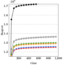
Cumulative regret comparison. We run the experiments 10 times, and calculate the average cumulative regret for each algorithm. The results plotted in Figure 3a show that LinUCB has the largest cumulative regret, indicating that the use of conversational feedbacks, either by querying items (Arm-Con) or by querying key-terms (Var-RS, ConUCB, Var-MRC, Var-LCR) can improve the learning speed of bandit, since they can learn parameters more accurately within the same number of iterations. Moreover, algorithms that query key-terms, i.e., Var-RS, ConUCB, Var-MRC, Var-LCR, have much smaller cumulative regret than Arm-Con, which asks the user’s preference on additional items. It is reasonable, because feedback on a key-term should be more informative than feedback on an arm. Finally, the ConUCB algorithm has the smallest cumulative regret, demonstrating the effectiveness of its key-term selection strategy.

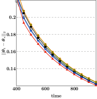
Accuracy of learned parameters. We next compare the accuracy of the learned parameters in different algorithms. For each algorithm, we calculate the average difference between the learned parameter vectors of users and the ground-truth parameter vectors of users, i.e., 1Nuu𝜽u,t𝜽u,21subscript𝑁𝑢subscript𝑢subscriptnormsubscript𝜽𝑢𝑡subscript𝜽𝑢2\frac{1}{N_{u}}\sum_{u}\|\bm{\theta}_{u,t}-\bm{\theta}_{u,*}\|_{2}, where 𝜽u,tsubscript𝜽𝑢𝑡\bm{\theta}_{u,t} and 𝜽u,subscript𝜽𝑢\bm{\theta}_{u,*} represent the learned and the ground-truth parameter vectors of user u𝑢u respectively. A smaller 1Nuu𝜽u,t𝜽u,21subscript𝑁𝑢subscript𝑢subscriptnormsubscript𝜽𝑢𝑡subscript𝜽𝑢2\frac{1}{N_{u}}\sum_{u}\|\bm{\theta}_{u,t}-\bm{\theta}_{u,*}\|_{2} implies a higher accuracy in learning of parameter vector. Figure 3b shows the average difference 1Nuu𝜽u,t𝜽u,21subscript𝑁𝑢subscript𝑢subscriptnormsubscript𝜽𝑢𝑡subscript𝜽𝑢2\frac{1}{N_{u}}\sum_{u}\|\bm{\theta}_{u,t}-\bm{\theta}_{u,*}\|_{2} in every 50 iterations. One can observe that for all algorithms, the values of 1Nuu𝜽u,t𝜽u,21subscript𝑁𝑢subscript𝑢subscriptnormsubscript𝜽𝑢𝑡subscript𝜽𝑢2\frac{1}{N_{u}}\sum_{u}\|\bm{\theta}_{u,t}-\bm{\theta}_{u,*}\|_{2} decrease in t𝑡t. That is, all algorithms can learn the parameters more accurately with more interactions with users. Moreover, ConUCB is the best algorithm in learning of the parameters.

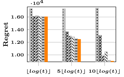
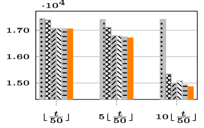
Impact of conversation frequency b(t)𝑏𝑡b(t). Next we study the impact of conversation frequency. In principle, key-term-level conversations should be less frequent than arm-level interactions, i.e., b(t)t𝑏𝑡𝑡b(t)\leq t. Thus we mainly consider two types of conversation frequency function b(t)𝑏𝑡b(t): (1) b(t)=Qllog(t)𝑏𝑡subscript𝑄𝑙𝑡b(t)=Q_{l}\lfloor\log(t)\rfloor: ask Qlsubscript𝑄𝑙Q_{l} questions every time, while the span between two consecutive conversations gets larger and larger; (2) b(t)=QltQq𝑏𝑡subscript𝑄𝑙𝑡subscript𝑄𝑞b(t)=Q_{l}\lfloor\frac{t}{Q_{q}}\rfloor: ask Qlsubscript𝑄𝑙Q_{l} questions per Qqsubscript𝑄𝑞Q_{q} iterations. For the first type of b(t)𝑏𝑡b(t), we vary the value of Qlsubscript𝑄𝑙Q_{l}, and obtain cumulative regrets at round 1000 shown in Figure 2a. For the second type of b(t)𝑏𝑡b(t), we set Qq=50subscript𝑄𝑞50Q_{q}=50, vary the value of Qlsubscript𝑄𝑙Q_{l}, and plot cumulative regrets at round 1000 in Figure 2b. We also run the experiments with Qq=20subscript𝑄𝑞20Q_{q}=20 and Qq=100subscript𝑄𝑞100Q_{q}=100, and the results are similar to that with Qq=50subscript𝑄𝑞50Q_{q}=50.

Figure 2b and Figure 2a show that asking more questions can help reduce the cumulative regrets more. For example, in Figure 2a, the cumulative regret is the largest when b(t)=log(t)𝑏𝑡𝑡b(t)=\lfloor\log(t)\rfloor, while the cumulative regret is the smallest when b(t)=10log(t)𝑏𝑡10𝑡b(t)=10\lfloor\log(t)\rfloor. Similarly, in Figure 2b, the cumulative regret is the largest when b(t)=t50𝑏𝑡𝑡50b(t)=\lfloor\frac{t}{50}\rfloor, while it is the smallest when b(t)=10t50𝑏𝑡10𝑡50b(t)=10\lfloor\frac{t}{50}\rfloor.

Comparing the cumulative regrets with b(t)=5log(t)𝑏𝑡5𝑡b(t)=5\lfloor\log(t)\rfloor and b(t)=5t50𝑏𝑡5𝑡50b(t)=5\lfloor\frac{t}{50}\rfloor, we can observe that although the agent asks more questions with b(t)=5t50𝑏𝑡5𝑡50b(t)=5\lfloor\frac{t}{50}\rfloor, its cumulative regret is much larger than that with b(t)=5log(t)𝑏𝑡5𝑡b(t)=5\lfloor\log(t)\rfloor. The reason seems to be that with b(t)=5log(t)𝑏𝑡5𝑡b(t)=5\lfloor\log(t)\rfloor the agent can ask more questions at the beginning, quickly capture users’ preference, and then gradually reduce the cumulative regret afterward.

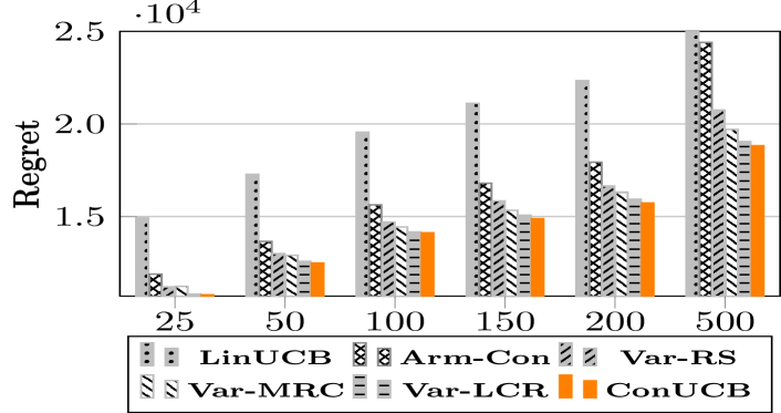
Impact of poolsize |𝒜t|subscript𝒜𝑡|\mathcal{A}_{t}|. We change the size of 𝒜tsubscript𝒜𝑡\mathcal{A}_{t} from 25 to 500 while fixing all the parameters as described in Section 4.1. Figure 2c plots the cumulative regrets under different poolsizes. One can observe that as the poolsize increases, the cumulative regrets of all algorithms also increase, since it is more difficult to select the best arm when the poolsize becomes larger. Again, we observe similar trends in different poolsizes: (1) Using conversational feedbacks, either by querying additional arms (Arm-Con), or by querying key-terms (Var-RS, Var-MRC, Var-LCR, ConUCB) can reduce regret; Querying key-terms is more effective and has smaller regrets than querying arms. (2) The regret of ConUCB is the smallest.
Refer to caption
(a) Effect of b(t)=Qllog(t)𝑏𝑡subscript𝑄𝑙𝑡b(t)=Q_{l}\lfloor\log(t)\rfloor
Refer to caption
(b) Effect of b(t)=Qlt50𝑏𝑡subscript𝑄𝑙𝑡50b(t)=Q_{l}\lfloor\frac{t}{50}\rfloor
Refer to caption
(c) Effect of poolsize
Figure 2. Effect of various factors: Figures (a) & (b) show the effect of b(t)𝑏𝑡b(t); Figure (c) shows the effect of poolsize.
Refer to caption
Refer to caption
(a) Cumulative regret on synthetic dataset
Refer to caption
(b) Accuracy of learned parameters
Refer to caption
(c) Cumulative regret on Yelp dataset
Refer to caption
(d) Normalized CTR on Toutiao dataset
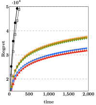
Figure 3. Experimental results on all datasets.

5. Experiments on Real Data

In this section, we describe empirical evaluations of the ConUCB algorithm on two real-world datasets.

5.1. Experiments on Yelp Dataset

Yelp dataset. The public Yelp dataset111http://www.yelp.com/academic_dataset contains users’ reviews of restaurants on Yelp. We only keep users with no less than 100 reviews, and restaurants with no less than 50 reviews. The final Yelp dataset has 1,998 users, 25,160 restaurants, and 342,237 reviews.

Experiment settings. We take each restaurant as an arm. Each restaurant in the dataset is associated with a number of categories. For example, one restaurant named “Garage” is associated with the following categories: { “Mexican”, “Burgers”, ”Gastropubs”}. We take each category as a key-term. Each arm is equally related to its associated key-terms. There are in total 1,004 categories in the dataset, i.e. |𝒦|=1004𝒦1004|\mathcal{K}|=1004. We construct 505050-dimensional arms’ contextual vectors via applying PCA on feature vectors generated from restaurants’ attributes, including: (1) geographic features: 330 different cities; (2) categorical features: 1,004 different categories; (3) average rating and total review count; (4) attributes: 34 different attributes, such as whether the restaurant serves alcohol or WIFI. We also normalize all the contextual vectors, i.e., 𝒙a2=1,asubscriptnormsubscript𝒙𝑎21for-all𝑎\|\bm{x}_{a}\|_{2}=1,\forall a. The original 5-scale ratings are converted to a binary-valued feedback between restaurants and users, i.e., high ratings (4 and 5) as positive(1) and low ratings ( 3absent3\leq 3) as negative(0). We derive users’ true parameters based on ridge regression. We fix the size of 𝒜tsubscript𝒜𝑡\mathcal{A}_{t} to 50. During the simulation, the true arm-level reward ra,tsubscript𝑟𝑎𝑡r_{a,t} as well as key-term level reward r~k,tsubscript~𝑟𝑘𝑡\tilde{r}_{k,t} are generated according to Eq. (2) and Eq. (4) respectively. Note that key-terms (i.e., categorical features) are part of arms’ feature sets, thus the information about key-terms is also available for all algorithms.

Evaluation results. We compare all six algorithms in terms of cumulative regret. We adopt the frequency function b(t)=5log(t)𝑏𝑡5𝑙𝑜𝑔𝑡b(t)=5\lfloor log(t)\rfloor. We run the experiments 10 times, and the average result for each algorithm is shown in Figure 3c. We observe similar results as those on the synthetic dataset. That is, all algorithms that query key-terms, i.e., Var-RS, Var-MRC, Var-LCR, ConUCB, have smaller cumulative regrets than LinUCB and Arm-Con. Moreover, the ConUCB algorithm has the smallest cumulative regret, followed by Var-LCR, and then Var-MRC and Var-RS.

5.2. Experiments on Toutiao Dataset

Toutiao dataset. This is a real-world news recommendation dataset, obtained from Toutiao222https://www.Toutiao.com/, which is the largest news recommendation platform in China. The dataset contains 2,000 users’ interaction records in December 2017. There are 1,746,335 news articles and 8,462,597 interaction records.

Experiment settings. We take each news article as an arm. Each article is associated with several categories, such as, “news_car” and “news_sports”. Each article is also associated with several keywords automatically extracted from the article. We filter the keywords occurring less than 1,000 times. In total, there are 2,38423842,384 keywords and 573 categories. We take them as key-terms 𝒦𝒦\mathcal{K}. We assume that an article is equally related to its associated key-terms. To get the contextual vector of an arm, we first represent the article by a vector of 3,469 features (e.g., topic distribution, categories, keywords, etc.). We then use PCA to conduct dimension reduction, and take the first 100 principal components as the contextual vectors, i.e., d=100𝑑100d=100. We infer each user’s feedback on an article through the user’s reading behavior: if the user reads the article, then the feedback is 1, otherwise the feedback is 0. The feedback is also the reward of the article. We infer each user’s feedback on key-terms by simulation. Specifically, we pre-process the interacted articles of the 2,000 users in November 2017 as above, and employ ridge regression to infer users’ true preference based on interaction records in the period. Then we generate the ground-truth key-term-level feedbacks according to Eq. (4). Note that the information about key-terms is also available for LinUCB and Arm-Con algorithms, in the sense that key-terms (i.e., categories, keywords) are in arms’ feature sets.

Comparison method. The unbiased offline evaluation protocol proposed in  (Li et al., 2011) is utilized to compare different algorithms. The unbiased offline evaluation protocol only works when the feedback in the system is collected under a random policy. Hence, we simulate the random policy of the system by generating a candidate pool as follows. At each round t𝑡t, we store the article presented to the user (atsubscript𝑎𝑡a_{t}) and its received feedback ratsubscript𝑟subscript𝑎𝑡r_{a_{t}}. Then we create 𝒜tsubscript𝒜𝑡\mathcal{A}_{t} by including the served article along with 49 extra articles the user has interacted with (hence |𝒜t|=50,tsubscript𝒜𝑡50for-all𝑡|\mathcal{A}_{t}|=50,\forall t). The 49 extra articles are drawn uniformly at random so that for any article a𝑎a the user interacted with, if a𝑎a occurs in some set 𝒜tsubscript𝒜𝑡\mathcal{A}_{t}, this article will be the one served by the system 1/50 of the times. The performance of algorithms is evaluated by Click Through-Rate (CTR), the ratio between the number of clicks an algorithm receives and the number of recommendations it makes. Specifically, we use the average CTR in every 500 iterations (not the cumulative CTR) as the evaluation metric. Following (Li et al., 2010), we normalize the resulting CTR from different algorithms by the corresponding logged random strategy’s CTR.

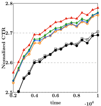
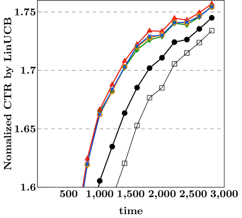
Evaluation results. Figure 3d shows the normalized CTRs of different algorithms over 2000 users. One can observe that algorithms that querying key-terms can achieve higher CTRs than LinUCB and Arm-Con. Again ConUCB achieves the best performance. Moreover, on the Toutiao dataset, Var-MRC and Var-LCR perform worse than Var-RS. This is because they tend to select key-terms related to a large group of arms repeatedly. One can also observe that Arm-Con only outperforms LinUCB slightly. This is because Toutiao dataset contains more negative feedbacks than positive feedbacks, and some negative feedbacks are caused by that a user has read something similar, rather than this user does not like the article. However, articles with such negative feedbacks may be queried by Arm-Con using additional questions with larger probability, due to articles with similar contents received positive feedbacks from the same user. This brings disturbance to the learning of the user’s parameter vector, decreasing the efficiency of additional questions.

6. Extension of Algorithm

ConUCB incorporates conversations into LinUCB. We demonstrate that the technique is generic and can be applied to other contextual bandit algorithms as well. Specifically, we show how to extend the hLinUCB algorithm (Wang et al., 2016) with conversational feedbacks.

Conversational hLinUCB. The hLinUCB algorithm (Wang et al., 2016) is one of the recent contextual bandit algorithms, which utilizes a set of l𝑙l-dimensional hidden features (𝒗alsubscript𝒗𝑎superscript𝑙\bm{v}_{a}\in\mathbb{R}^{l}) that affects the expected reward, in addition to the contextual features (𝒙a,tdsubscript𝒙𝑎𝑡superscript𝑑\bm{x}_{a,t}\in\mathbb{R}^{d}). Formally,

(9) ra,t=(𝒙a,t,𝒗a)T𝜽u+ηt,subscript𝑟𝑎𝑡superscriptsubscript𝒙𝑎𝑡subscript𝒗𝑎𝑇subscript𝜽𝑢subscript𝜂𝑡\displaystyle\textstyle r_{a,t}=(\bm{x}_{a,t},\bm{v}_{a})^{T}\bm{\theta}_{u}+\eta_{t},\vspace{-6mm}

where 𝜽ul+dsubscript𝜽𝑢superscript𝑙𝑑\bm{\theta}_{u}\in\mathbb{R}^{l+d} is the parameter of user u𝑢u, and ηtsubscript𝜂𝑡\eta_{t} is drawn from a zero-mean Gaussian distribution 𝒩(0,γ2)𝒩0superscript𝛾2\mathcal{N}(0,\gamma^{2}).

We then design the hConUCB algorithm to extend the hLinUCB algorithm to incorporate conversational feedbacks. At round t𝑡t, hConUCB first infers user u𝑢u’s current key-term-level preference 𝜽~u,tsubscriptbold-~𝜽𝑢𝑡\bm{\tilde{\theta}}_{u,t} solely based on her conversational feedbacks, and then use 𝜽~u,tsubscriptbold-~𝜽𝑢𝑡\bm{\tilde{\theta}}_{u,t} to guide the learning of user u𝑢u’s arm-level preference 𝜽^u,tsubscriptbold-^𝜽𝑢𝑡\bm{\hat{\theta}}_{u,t}, with the estimated hidden features {𝒗^a,t}a𝒜subscriptsubscriptbold-^𝒗𝑎𝑡𝑎𝒜\{\bm{\hat{v}}_{a,t}\}_{a\in\mathcal{A}} fixed. Then, fixing 𝜽~u,tsubscriptbold-~𝜽𝑢𝑡\bm{\tilde{\theta}}_{u,t} and 𝜽^u,tsubscriptbold-^𝜽𝑢𝑡\bm{\hat{\theta}}_{u,t}, we use both conversational feedbacks and arm-level feedbacks to update the hidden features of arms {𝒗^a,t}a𝒜subscriptsubscriptbold-^𝒗𝑎𝑡𝑎𝒜\{\bm{\hat{v}}_{a,t}\}_{a\in\mathcal{A}}. One can also derive the confidence bound following a similar procedure as in Lemma 1, and choose the arm with the maximal upper confidence bound value. The key-term-selection strategy of hConUCB follows the procedure in Theorem 2. Moreover, we modify the baselines in Section 4.1 in a similar way. For example, similar to Arm-Con, the hArm-Con algorithm conducts conversations by querying whether a user likes the item selected by hLinUCB.

Experiment evaluations. We then compare hConUCB with the modified baselines on the previous three datasets. The experimental settings on the three datasets are the same as those in Section 4 and in Section 5. The only difference is that in this section, features are randomly partitioned into an observable part and a hidden part. We fix the dimensionaliy l𝑙l of hidden features to 555, and set the dimensionality d𝑑d of observable features to 454545 on synthetic dataset and Yelp dataset, and d=95𝑑95d=95 on Toutiao dataset. We set γ=0.1𝛾0.1\gamma=0.1. Note that only observable features are showed to the algorithms. The arm-level feedback ra,tsubscript𝑟𝑎𝑡r_{a,t} and the key-term-level feedback r~k,tsubscript~𝑟𝑘𝑡\tilde{r}_{k,t} are generated similarly as in Section 4 and in Section 5, except the arm-level reward model is in Eq. (9).

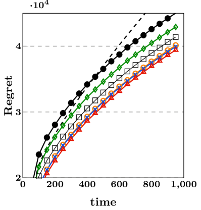
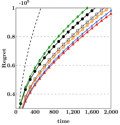
Figure 4a and 4b show the cumulative regrets (defined in Eq. (10)) on synthetic dataset and Yelp dataset respectively. One can observe that on both datasets, the algorithms that query key-terms except hVar-RS outperform LinUCB, hLinUCB and hArm-Con. Moreover, hConUCB has the smallest cumulative regret. The poor performance of hVar-RS is because randomly selecting key-terms cannot effectively contribute to the inference of arms’ hidden features.

For the experiments on Toutiao dataset, we normalize the CTRs from different algorithms by the corresponding CTR of LinUCB. Figure 4c shows the normalized CTRs of different algorithms on Toutiao dataset. The values on the vertical axis in Figure 4c are all larger than 111, indicating that all the algorithms outperform LinUCB. Also, we can observe that all algorithms that query key-terms have higher CTRs than hLinUCB and hArm-Con, and hConUCB achieves the highest CTR. Moreover, in this experiment, the performance of hArm-Con is worse than that of hLinUCB. The reason might be the same as that Arm-Con does not outperform LinUCB, as shown in Figure  3d. In summary, the results demonstrate the effectiveness of conversational mechanism incorporated into bandit algorithms.
Refer to caption
(a) synthetic dataset
Refer to caption
(b) Yelp dataset
Refer to caption
(c) Toutiao dataset
Refer to caption
Figure 4. Experimental results of conversational hLinUCB.

7. Related Work

To the best of our knowledge, this is the first work to study the conversational contextual bandit problem. Our work is closely related to the following two lines of research.

Contextual bandit algorithms. Contextual bandit is a popular technique to address the exploration-exploitation trade-off, in various application tasks such as recommendation. LinUCB (Li et al., 2010) and Thompson Sampling (Agrawal and Goyal, 2013) are two representative algorithms for contextual bandits. A large number of algorithms have been proposed to accelerate the learning speed of LinUCB. For example, Bianchi et. al. (Cesa-Bianchi et al., 2013; Wu et al., 2016; Li et al., 2016) leverage relationship among users. Wang et. al. (Wang et al., 2016) learn hidden features, and Zheng et.al. (Zeng et al., 2016) make use of a time-changing reward function. The CoFineUCB (Yue et al., 2012) algorithm proposed by Yue et. al. performs a coarse-to-fine hierarchical exploration. Different from them, our work tries to accelerate the learning speed through conversation. More importantly, as shown in Section 6, our approach is generic and can be applied to many existing algorithms.

It should be possible to incorporate the conversation mechanism into Thompson Sampling (Agrawal and Goyal, 2013). Thompson Sampling is a probability matching algorithm that samples 𝜽tsubscript𝜽𝑡\bm{\theta}_{t} from the posterior distribution. Thus, one can define a hierarchical sampling approach that first samples 𝜽~tsubscriptbold-~𝜽𝑡\bm{\tilde{\theta}}_{t} according to conversational feedbacks, and then samples 𝜽tsubscript𝜽𝑡\bm{\theta}_{t} around 𝜽~tsubscriptbold-~𝜽𝑡\bm{\tilde{\theta}}_{t} while considering arm-level feedbacks.

Conversational recommender systems. Christakopoulou et. al. (Christakopoulou et al., 2016) introduce the idea of conversational recommender systems. They conduct conversations by querying whether the user likes the items selected by the bandits algorithm. As shown in this paper, item-level conversations are less efficient than key-term-level conversations. Other researchers (Zhang et al., 2018; Sun and Zhang, 2018; Christakopoulou et al., 2018) further leverage recent advances in natural language understanding to generate conversations and assist recommendation. Their works utilize conversation in user preference learning (via deep learning or reinforcement learning) without theoretical guarantee, while our work utilizes conversation to speed up contextual bandit learning with theoretical guarantee. Yu et. al. (Yu et al., 2019) propose a dialog approach to speed up bandit learning in recommender systems. Their dialog approach recommends multiple items to the user and the user needs to provide feedback on why she likes or dislikes the recommended items. In this paper, we explore another approach of using conversations, i.e, querying key-terms occasionally to actively explore the user’s preference. Bu et. al (Bu and Small, 2018) also leverage conversations to assist item recommendation, however, their algorithm is only applied to offline learning, while our algorithm, based on the bandit technique, is an online learning algorithm. Furthermore, our algorithm adaptively optimizes the question strategy through interactions and conversations.

8. Conclusion

We formulate the conversational contextual bandit problem by incorporating a conversational mechanism into contextual bandit. We design the ConUCB algorithm to adaptively optimize the arm selection strategy and the key-term selection strategy through conversations and arm-level interactions with the user. Theoretical analysis shows that ConUCB can achieve a lower regret upper bound. Extensive experiments on synthetic dataset, real datasets from Yelp and Toutiao demonstrate that ConUCB indeed has a faster learning speed. The generality of the approach of incorporating conversations into bandit algorithms is also demonstrated.

9. Acknowledgments

The work is supported by National Nature Science Foundation of China (61902042) and the GRF 14201819.

10. Appendix

Proof of Lemma 1:

Proof.

According to the closed-form solution of 𝜽tsubscript𝜽𝑡\bm{\theta}_{t}, we can get:

𝜽𝒕=𝑴t1𝒃tsubscript𝜽𝒕superscriptsubscript𝑴𝑡1subscript𝒃𝑡\displaystyle\textstyle\bm{\theta_{t}}=\bm{M}_{t}^{-1}\bm{b}_{t}
=(λτ=1t1𝒙a,τ𝒙a,τT+(1λ)𝑰)1(λτ=1t1𝒙a,τra,τ+(1λ)𝜽~t)absentsuperscript𝜆superscriptsubscript𝜏1𝑡1subscript𝒙𝑎𝜏superscriptsubscript𝒙𝑎𝜏𝑇1𝜆𝑰1𝜆superscriptsubscript𝜏1𝑡1subscript𝒙𝑎𝜏subscript𝑟𝑎𝜏1𝜆subscriptbold-~𝜽𝑡\displaystyle\textstyle=\left(\lambda\sum_{\tau=1}^{t-1}\bm{x}_{a,\tau}\bm{x}_{a,\tau}^{T}+(1-\lambda)\bm{I}\right)^{-1}(\lambda\sum_{\tau=1}^{t-1}\bm{x}_{a,\tau}r_{a,\tau}+(1-\lambda)\bm{\tilde{\theta}}_{t})
=𝜽(1λ)𝑴t1𝜽+λ𝑴t1(τ=1t1𝒙a,τϵτ)+(1λ)𝑴t1𝜽~t.absentsubscript𝜽1𝜆superscriptsubscript𝑴𝑡1subscript𝜽𝜆superscriptsubscript𝑴𝑡1superscriptsubscript𝜏1𝑡1subscript𝒙𝑎𝜏subscriptitalic-ϵ𝜏1𝜆superscriptsubscript𝑴𝑡1subscriptbold-~𝜽𝑡\displaystyle\textstyle=\bm{\theta_{*}}-(1-\lambda)\bm{M}_{t}^{-1}\bm{\theta_{*}}+\lambda\bm{M}_{t}^{-1}(\sum_{\tau=1}^{t-1}\bm{x}_{a,\tau}\epsilon_{\tau})+(1-\lambda)\bm{M}_{t}^{-1}\bm{\tilde{\theta}}_{t}.

The equality holds since ra,τ=𝒙a,τT𝜽+ϵτsubscript𝑟𝑎𝜏superscriptsubscript𝒙𝑎𝜏𝑇subscript𝜽subscriptitalic-ϵ𝜏r_{a,\tau}=\bm{x}_{a,\tau}^{T}\bm{\theta}_{*}+\epsilon_{\tau}. With 𝜽𝜽~subscript𝜽subscriptbold-~𝜽\bm{\theta}_{*}\approx\bm{\tilde{\theta}}_{*},

(10) 𝜽t𝜽subscript𝜽𝑡subscript𝜽\displaystyle\textstyle\quad\bm{\theta}_{t}-\bm{\theta}_{*} =(1λ)𝑴t1(𝜽~t𝜽~)+λ𝑴t1(τ=1t1𝒙a,τϵτ).absent1𝜆superscriptsubscript𝑴𝑡1subscriptbold-~𝜽𝑡subscriptbold-~𝜽𝜆superscriptsubscript𝑴𝑡1superscriptsubscript𝜏1𝑡1subscript𝒙𝑎𝜏subscriptitalic-ϵ𝜏\displaystyle\textstyle=(1-\lambda)\bm{M}_{t}^{-1}(\bm{\tilde{\theta}}_{t}-\bm{\tilde{\theta}}_{*})+\lambda\bm{M}_{t}^{-1}(\sum_{\tau=1}^{t-1}\bm{x}_{a,\tau}\epsilon_{\tau}).

Thus, with 𝜽~t𝜽~𝑴~tα~tsubscriptnormsubscriptbold-~𝜽𝑡subscriptbold-~𝜽subscriptbold-~𝑴𝑡subscript~𝛼𝑡\|\bm{\tilde{\theta}}_{t}-\bm{\tilde{\theta}}_{*}\|_{\bm{\tilde{M}}_{t}}\leq\tilde{\alpha}_{t}, we can get:

|𝒙a,tT𝜽𝒕𝒙a,tT𝜽|superscriptsubscript𝒙𝑎𝑡𝑇subscript𝜽𝒕superscriptsubscript𝒙𝑎𝑡𝑇subscript𝜽\displaystyle\textstyle|\bm{x}_{a,t}^{T}\bm{\theta_{t}}-\bm{x}_{a,t}^{T}\bm{\theta}_{*}|
=(1λ)|𝒙a,tT𝑴t1(𝜽~t𝜽~)|+λ|𝒙a,tT𝑴t1(τ=1t1𝒙a,τϵτ)|absent1𝜆superscriptsubscript𝒙𝑎𝑡𝑇superscriptsubscript𝑴𝑡1subscriptbold-~𝜽𝑡subscriptbold-~𝜽𝜆superscriptsubscript𝒙𝑎𝑡𝑇superscriptsubscript𝑴𝑡1superscriptsubscript𝜏1𝑡1subscript𝒙𝑎𝜏subscriptitalic-ϵ𝜏\displaystyle=(1-\lambda)|\bm{x}_{a,t}^{T}\bm{M}_{t}^{-1}(\bm{\tilde{\theta}}_{t}-\bm{\tilde{\theta}}_{*})|+\lambda|\bm{x}_{a,t}^{T}\bm{M}_{t}^{-1}(\sum_{\tau=1}^{t-1}\bm{x}_{a,\tau}\epsilon_{\tau})|
(1λ)α~t𝒙a,tT𝑴t1𝑴~t1+λ𝒙a,t𝑴t1τ=1t1𝒙a,τϵτ𝑴t1.absent1𝜆subscript~𝛼𝑡subscriptnormsuperscriptsubscript𝒙𝑎𝑡𝑇superscriptsubscript𝑴𝑡1superscriptsubscriptbold-~𝑴𝑡1𝜆subscriptnormsubscript𝒙𝑎𝑡superscriptsubscript𝑴𝑡1subscriptnormsuperscriptsubscript𝜏1𝑡1subscript𝒙𝑎𝜏subscriptitalic-ϵ𝜏superscriptsubscript𝑴𝑡1\displaystyle\textstyle\leq(1-\lambda)\tilde{\alpha}_{t}\|\bm{x}_{a,t}^{T}\bm{M}_{t}^{-1}\|_{\bm{\tilde{M}}_{t}^{-1}}+\lambda\|\bm{x}_{a,t}\|_{\bm{M}_{t}^{-1}}\|\sum_{\tau=1}^{t-1}\bm{x}_{a,\tau}\epsilon_{\tau}\|_{\bm{M}_{t}^{-1}}.

Let αtsubscript𝛼𝑡\alpha_{t} denote the upper bound of τ=1t1𝒙a,τϵτ𝑴t1subscriptnormsuperscriptsubscript𝜏1𝑡1subscript𝒙𝑎𝜏subscriptitalic-ϵ𝜏superscriptsubscript𝑴𝑡1\|\sum_{\tau=1}^{t-1}\bm{x}_{a,\tau}\epsilon_{\tau}\|_{\bm{M}_{t}^{-1}}, then Theorem 1 in paper (Abbasi-Yadkori et al., 2011) suggests that

αt=2log(det(𝑴t)1/2det((1λ)𝑰)1/2σ)dlog((1+λt(1λ)d)/σ).subscript𝛼𝑡2superscriptsubscript𝑴𝑡12superscript1𝜆𝑰12𝜎𝑑1𝜆𝑡1𝜆𝑑𝜎\displaystyle\textstyle\alpha_{t}=\sqrt{2\log\left(\frac{\det(\bm{M}_{t})^{1/2}\det((1-\lambda)\bm{I})^{-1/2}}{\sigma}\right)}\leq\sqrt{d\log\left((1+\frac{\lambda t}{(1-\lambda)d})/\sigma\right)}.

This proof is then complete. ∎

Proof of Theorem 2:

Proof.

According to Theorem 5, to minimize 𝔼[𝑿t𝜽t𝑿t𝜽22]𝔼delimited-[]superscriptsubscriptnormsubscript𝑿𝑡subscript𝜽𝑡subscript𝑿𝑡subscript𝜽22\mathbb{E}[\|\bm{X}_{t}\bm{\theta}_{t}-\bm{X}_{t}\bm{\theta}_{*}\|_{2}^{2}], the key-term selection strategy needs to select key-term k𝑘k to minimize

tr(𝑿t𝑴t1(𝑴~t1+𝒙~k,t𝒙~k,tT)1𝑴t1𝑿tT).trsubscript𝑿𝑡superscriptsubscript𝑴𝑡1superscriptsubscriptbold-~𝑴𝑡1subscriptbold-~𝒙𝑘𝑡superscriptsubscriptbold-~𝒙𝑘𝑡𝑇1superscriptsubscript𝑴𝑡1superscriptsubscript𝑿𝑡𝑇\operatorname{tr}\left(\bm{X}_{t}\bm{M}_{t}^{-1}(\bm{\tilde{M}}_{t-1}+\bm{\tilde{x}}_{k,t}\bm{\tilde{x}}_{k,t}^{T})^{-1}\bm{M}_{t}^{-1}\bm{X}_{t}^{T}\right).

Then, using Woodbury matrix identity, it is equal to minimize:

tr(𝑿t𝑴t1𝑴~t11𝑴t1𝑿tT)𝑿t𝑴t1𝑴~t11𝒙~k,t221+𝒙~k,tT𝑴~t11𝒙~k,t.trsubscript𝑿𝑡superscriptsubscript𝑴𝑡1superscriptsubscriptbold-~𝑴𝑡11superscriptsubscript𝑴𝑡1superscriptsubscript𝑿𝑡𝑇superscriptsubscriptnormsubscript𝑿𝑡superscriptsubscript𝑴𝑡1superscriptsubscriptbold-~𝑴𝑡11subscriptbold-~𝒙𝑘𝑡221superscriptsubscriptbold-~𝒙𝑘𝑡𝑇superscriptsubscriptbold-~𝑴𝑡11subscriptbold-~𝒙𝑘𝑡\displaystyle\textstyle\operatorname{tr}\left(\bm{X}_{t}\bm{M}_{t}^{-1}\bm{\tilde{M}}_{t-1}^{-1}\bm{M}_{t}^{-1}\bm{X}_{t}^{T}\right)-\frac{\|\bm{X}_{t}\bm{M}_{t}^{-1}\bm{\tilde{M}}_{t-1}^{-1}\bm{\tilde{x}}_{k,t}\|_{2}^{2}}{1+\bm{\tilde{x}}_{k,t}^{T}\bm{\tilde{M}}_{t-1}^{-1}\bm{\tilde{x}}_{k,t}}.

With the interaction history, tr(𝑿t𝑴t1𝑴~t11𝑴t1𝑿tT)trsubscript𝑿𝑡superscriptsubscript𝑴𝑡1superscriptsubscriptbold-~𝑴𝑡11superscriptsubscript𝑴𝑡1superscriptsubscript𝑿𝑡𝑇\operatorname{tr}\left(\bm{X}_{t}\bm{M}_{t}^{-1}\bm{\tilde{M}}_{t-1}^{-1}\bm{M}_{t}^{-1}\bm{X}_{t}^{T}\right) is a constant. Thus, the proof is complete. ∎

Theorem 5.

Given the interaction history at both arm-level and key-term level up to round t𝑡t, we have:

(1)mink𝔼[𝑿t𝜽t𝑿t𝜽22]mink𝔼[𝑿t𝑴t1(𝜽~t𝜽~)22].1subscript𝑘𝔼delimited-[]superscriptsubscriptnormsubscript𝑿𝑡subscript𝜽𝑡subscript𝑿𝑡subscript𝜽22subscript𝑘𝔼delimited-[]superscriptsubscriptnormsubscript𝑿𝑡superscriptsubscript𝑴𝑡1subscriptbold-~𝜽𝑡subscriptbold-~𝜽22\displaystyle(1)\quad\min_{k}\mathbb{E}[\|\bm{X}_{t}\bm{\theta}_{t}-\bm{X}_{t}\bm{\theta}_{*}\|_{2}^{2}]\Leftrightarrow\min_{k}\mathbb{E}[\|\bm{X}_{t}\bm{M}_{t}^{-1}(\bm{\tilde{\theta}}_{t}-\bm{\tilde{\theta}}_{*})\|_{2}^{2}].
(2)𝔼[𝑿t𝑴t1(𝜽~t𝜽~)22](𝜽22+1)tr(𝑿t𝑴t1𝑴~t1𝑴t1𝑿tT).2𝔼delimited-[]superscriptsubscriptnormsubscript𝑿𝑡superscriptsubscript𝑴𝑡1subscriptbold-~𝜽𝑡subscriptbold-~𝜽22superscriptsubscriptnormsubscript𝜽221trsubscript𝑿𝑡superscriptsubscript𝑴𝑡1superscriptsubscriptbold-~𝑴𝑡1superscriptsubscript𝑴𝑡1superscriptsubscript𝑿𝑡𝑇\displaystyle(2)\quad\mathbb{E}[\|\bm{X}_{t}\bm{M}_{t}^{-1}(\bm{\tilde{\theta}}_{t}-\bm{\tilde{\theta}}_{*})\|_{2}^{2}]\leq(\|\bm{\theta}_{*}\|_{2}^{2}+1)\operatorname{tr}\left(\bm{X}_{t}\bm{M}_{t}^{-1}\bm{\tilde{M}}_{t}^{-1}\bm{M}_{t}^{-1}\bm{X}_{t}^{T}\right).
Proof.

With Eq. (10), we can get:

mink𝔼𝑿t𝜽t𝑿t𝜽22subscript𝑘𝔼superscriptsubscriptnormsubscript𝑿𝑡subscript𝜽𝑡subscript𝑿𝑡subscript𝜽22\displaystyle\quad\textstyle\min_{k}\mathbb{E}\|\bm{X}_{t}\bm{\theta}_{t}-\bm{X}_{t}\bm{\theta}_{*}\|_{2}^{2}
=mink𝔼(1λ)𝑿t𝑴t1(𝜽~t𝜽~)+λ𝑿t𝑴t1(τ=1t1𝒙τϵτ).absentsubscript𝑘𝔼norm1𝜆subscript𝑿𝑡superscriptsubscript𝑴𝑡1subscriptbold-~𝜽𝑡subscriptbold-~𝜽𝜆subscript𝑿𝑡superscriptsubscript𝑴𝑡1superscriptsubscript𝜏1𝑡1subscript𝒙𝜏subscriptitalic-ϵ𝜏\displaystyle\textstyle=\min_{k}\mathbb{E}\|(1-\lambda)\bm{X}_{t}\bm{M}_{t}^{-1}(\bm{\tilde{\theta}}_{t}-\bm{\tilde{\theta}}_{*})+\lambda\bm{X}_{t}\bm{M}_{t}^{-1}(\sum_{\tau=1}^{t-1}\bm{x}_{\tau}\epsilon_{\tau})\|.

Note that key-term selection does not affect {ϵτ}τ=1t1superscriptsubscriptsubscriptitalic-ϵ𝜏𝜏1𝑡1\{\epsilon_{\tau}\}_{\tau=1}^{t-1} , thus we can get the first observation:

mink𝔼𝑿t𝜽t𝑿t𝜽22mink𝔼𝑿t𝑴t1(𝜽~t𝜽~)22.subscript𝑘𝔼superscriptsubscriptnormsubscript𝑿𝑡subscript𝜽𝑡subscript𝑿𝑡subscript𝜽22subscript𝑘𝔼superscriptsubscriptnormsubscript𝑿𝑡superscriptsubscript𝑴𝑡1subscriptbold-~𝜽𝑡subscriptbold-~𝜽22\displaystyle\textstyle\min_{k}\mathbb{E}\|\bm{X}_{t}\bm{\theta}_{t}-\bm{X}_{t}\bm{\theta}_{*}\|_{2}^{2}\Leftrightarrow\min_{k}\mathbb{E}\|\bm{X}_{t}\bm{M}_{t}^{-1}(\bm{\tilde{\theta}}_{t}-\bm{\tilde{\theta}}_{*})\|_{2}^{2}.

For the second observation, according to the closed-form of 𝜽~tsubscriptbold-~𝜽𝑡\bm{\tilde{\theta}}_{t}, we can further infer that:

𝜽~t𝜽~=λ~𝑴~t1𝜽~+𝑴~t1(τ=1tk𝒦τ𝒙~k,τϵ~k,τ).subscriptbold-~𝜽𝑡subscriptbold-~𝜽~𝜆superscriptsubscriptbold-~𝑴𝑡1subscriptbold-~𝜽superscriptsubscriptbold-~𝑴𝑡1superscriptsubscript𝜏1𝑡subscript𝑘subscript𝒦𝜏subscriptbold-~𝒙𝑘𝜏subscript~italic-ϵ𝑘𝜏\displaystyle\textstyle\bm{\tilde{\theta}}_{t}-\bm{\tilde{\theta}}_{*}=-\tilde{\lambda}\bm{\tilde{M}}_{t}^{-1}\bm{\tilde{\theta}}_{*}+\bm{\tilde{M}}_{t}^{-1}\left(\sum_{\tau=1}^{t}\sum_{k\in\mathcal{K}_{\tau}}\bm{\tilde{x}}_{k,\tau}\tilde{\epsilon}_{k,\tau}\right).

Thus, we can get:

𝔼𝑿t𝑴t1(𝜽~t𝜽~)22𝔼superscriptsubscriptnormsubscript𝑿𝑡superscriptsubscript𝑴𝑡1subscriptbold-~𝜽𝑡subscriptbold-~𝜽22\displaystyle\textstyle\mathbb{E}\|\bm{X}_{t}\bm{M}_{t}^{-1}(\bm{\tilde{\theta}}_{t}-\bm{\tilde{\theta}}_{*})\|_{2}^{2}
λ~𝑿t𝑴t1𝑴~t1𝜽~22A1+𝔼𝑿t𝑴t1𝑴~t1(τ=1tk𝒦τ𝒙~k,τϵ~k,τ)22A2absent~𝜆subscriptsuperscriptsubscriptnormsubscript𝑿𝑡superscriptsubscript𝑴𝑡1superscriptsubscriptbold-~𝑴𝑡1subscriptbold-~𝜽22subscript𝐴1subscript𝔼superscriptsubscriptnormsubscript𝑿𝑡superscriptsubscript𝑴𝑡1superscriptsubscriptbold-~𝑴𝑡1superscriptsubscript𝜏1𝑡subscript𝑘subscript𝒦𝜏subscriptbold-~𝒙𝑘𝜏subscript~italic-ϵ𝑘𝜏22subscript𝐴2\displaystyle\textstyle\leq\tilde{\lambda}\underbrace{\|\bm{X}_{t}\bm{M}_{t}^{-1}\bm{\tilde{M}}_{t}^{-1}\bm{\tilde{\theta}}_{*}\|_{2}^{2}}_{A_{1}}+\underbrace{\mathbb{E}\|\bm{X}_{t}\bm{M}_{t}^{-1}\bm{\tilde{M}}_{t}^{-1}(\sum_{\tau=1}^{t}\sum_{k\in\mathcal{K}_{\tau}}\bm{\tilde{x}}_{k,\tau}\tilde{\epsilon}_{k,\tau})\|_{2}^{2}}_{A_{2}}
  • Bound A1subscript𝐴1A_{1}. The first term is bounded by:

    𝑿t𝑴t1𝑴~t1𝜽~22superscriptsubscriptnormsubscript𝑿𝑡superscriptsubscript𝑴𝑡1superscriptsubscriptbold-~𝑴𝑡1subscriptbold-~𝜽22\displaystyle\textstyle\|\bm{X}_{t}\bm{M}_{t}^{-1}\bm{\tilde{M}}_{t}^{-1}\bm{\tilde{\theta}}_{*}\|_{2}^{2} 𝑿t𝑴t1𝑴~t1/2F2𝑴~t1/2𝜽~22absentsuperscriptsubscriptnormsubscript𝑿𝑡superscriptsubscript𝑴𝑡1superscriptsubscriptbold-~𝑴𝑡12𝐹2superscriptsubscriptnormsuperscriptsubscriptbold-~𝑴𝑡12subscriptbold-~𝜽22\displaystyle\textstyle\leq\|\bm{X}_{t}\bm{M}_{t}^{-1}\bm{\tilde{M}}_{t}^{-1/2}\|_{F}^{2}\|\bm{\tilde{M}}_{t}^{-1/2}\bm{\tilde{\theta}}_{*}\|_{2}^{2}
    𝜽~22λ~tr(𝑿t𝑴t1𝑴~t1𝑴t1𝑿tT)absentsuperscriptsubscriptnormsubscriptbold-~𝜽22~𝜆trsubscript𝑿𝑡superscriptsubscript𝑴𝑡1superscriptsubscriptbold-~𝑴𝑡1superscriptsubscript𝑴𝑡1superscriptsubscript𝑿𝑡𝑇\displaystyle\textstyle\leq\frac{\|\bm{\tilde{\theta}}_{*}\|_{2}^{2}}{\tilde{\lambda}}\operatorname{tr}(\bm{X}_{t}\bm{M}_{t}^{-1}\bm{\tilde{M}}_{t}^{-1}\bm{M}_{t}^{-1}\bm{X}_{t}^{T})
  • Bound A2subscript𝐴2A_{2}. We denote τ=1tk𝒦τ𝒙~k,τϵ~k,τ=𝑿~tϵ~tsuperscriptsubscript𝜏1𝑡subscript𝑘subscript𝒦𝜏subscriptbold-~𝒙𝑘𝜏subscript~italic-ϵ𝑘𝜏subscriptbold-~𝑿𝑡subscriptbold-~bold-italic-ϵ𝑡\sum_{\tau=1}^{t}\sum_{k\in\mathcal{K}_{\tau}}\bm{\tilde{x}}_{k,\tau}\tilde{\epsilon}_{k,\tau}=\bm{\tilde{X}}_{t}\bm{\tilde{\epsilon}}_{t}, where 𝑿~tRd×b(t)subscriptbold-~𝑿𝑡superscript𝑅𝑑𝑏𝑡\bm{\tilde{X}}_{t}\in R^{d\times b(t)}. The second term is bounded by:

    𝔼𝑿t𝑴t1𝑴~t1(τ=1tk𝒦τ𝒙~k,τϵ~k,τ)22𝔼superscriptsubscriptnormsubscript𝑿𝑡superscriptsubscript𝑴𝑡1superscriptsubscriptbold-~𝑴𝑡1superscriptsubscript𝜏1𝑡subscript𝑘subscript𝒦𝜏subscriptbold-~𝒙𝑘𝜏subscript~italic-ϵ𝑘𝜏22\displaystyle\textstyle\mathbb{E}\|\bm{X}_{t}\bm{M}_{t}^{-1}\bm{\tilde{M}}_{t}^{-1}(\sum_{\tau=1}^{t}\sum_{k\in\mathcal{K}_{\tau}}\bm{\tilde{x}}_{k,\tau}\tilde{\epsilon}_{k,\tau})\|_{2}^{2}
    =𝔼[tr(𝑿t𝑴t1𝑴~t1𝑿~tϵ~tϵ~tT𝑿~tT𝑴~t1𝑴t1𝑿tT)]absent𝔼delimited-[]trsubscript𝑿𝑡superscriptsubscript𝑴𝑡1superscriptsubscriptbold-~𝑴𝑡1subscriptbold-~𝑿𝑡subscriptbold-~bold-italic-ϵ𝑡superscriptsubscriptbold-~bold-italic-ϵ𝑡𝑇superscriptsubscriptbold-~𝑿𝑡𝑇superscriptsubscriptbold-~𝑴𝑡1superscriptsubscript𝑴𝑡1superscriptsubscript𝑿𝑡𝑇\displaystyle\textstyle=\mathbb{E}[\operatorname{tr}(\bm{X}_{t}\bm{M}_{t}^{-1}\bm{\tilde{M}}_{t}^{-1}\bm{\tilde{X}}_{t}\bm{\tilde{\epsilon}}_{t}\bm{\tilde{\epsilon}}_{t}^{T}\bm{\tilde{X}}_{t}^{T}\bm{\tilde{M}}_{t}^{-1}\bm{M}_{t}^{-1}\bm{X}_{t}^{T})]
    tr(𝑿t𝑴t1𝑴~t1𝑴t1𝑿tT)absenttrsubscript𝑿𝑡superscriptsubscript𝑴𝑡1superscriptsubscriptbold-~𝑴𝑡1superscriptsubscript𝑴𝑡1superscriptsubscript𝑿𝑡𝑇\displaystyle\textstyle\leq\operatorname{tr}(\bm{X}_{t}\bm{M}_{t}^{-1}\bm{\tilde{M}}_{t}^{-1}\bm{M}_{t}^{-1}\bm{X}_{t}^{T})

    The first inequality is due to 𝔼[ϵ~tϵ~tT]I𝔼delimited-[]subscriptbold-~bold-italic-ϵ𝑡superscriptsubscriptbold-~bold-italic-ϵ𝑡𝑇𝐼\mathbb{E}[\bm{\tilde{\epsilon}}_{t}\bm{\tilde{\epsilon}}_{t}^{T}]\leq I.

Finally, with 𝜽~𝜽subscriptbold-~𝜽subscript𝜽\bm{\tilde{\theta}}_{*}\approx\bm{\theta}_{*}, we can finish the proof. ∎

Proof of Lemma 3:

Proof.

In the following analysis, we take 𝒙~k,τ=a𝒜wa,k𝒙a,τa𝒜wa,ksubscriptbold-~𝒙𝑘𝜏subscript𝑎𝒜subscript𝑤𝑎𝑘subscript𝒙𝑎𝜏subscript𝑎𝒜subscript𝑤𝑎𝑘\bm{\tilde{x}}_{k,\tau}=\frac{\sum_{a\in\mathcal{A}}w_{a,k}\bm{x}_{a,\tau}}{\sum_{a\in\mathcal{A}}w_{a,k}}.

𝜽~tsubscriptbold-~𝜽𝑡\displaystyle\textstyle\bm{\tilde{\theta}}_{t} =𝑴~𝒕1𝒃tabsentsuperscriptsubscriptbold-~𝑴𝒕1subscript𝒃𝑡\displaystyle\textstyle=\bm{\tilde{M}_{t}}^{-1}\bm{b}_{t}
=𝜽~λ~𝑴~t1𝜽~+𝑴~t1(τ=1tk𝒦τ𝒙~k,τϵ~k,τ)absentsubscriptbold-~𝜽~𝜆superscriptsubscriptbold-~𝑴𝑡1subscriptbold-~𝜽superscriptsubscriptbold-~𝑴𝑡1superscriptsubscript𝜏1𝑡subscript𝑘subscript𝒦𝜏subscriptbold-~𝒙𝑘𝜏subscript~italic-ϵ𝑘𝜏\displaystyle\textstyle=\bm{\tilde{\theta}}_{*}-\tilde{\lambda}\bm{\tilde{M}}_{t}^{-1}\bm{\tilde{\theta}}_{*}+\bm{\tilde{M}}_{t}^{-1}\left(\sum_{\tau=1}^{t}\sum_{k\in\mathcal{K}_{\tau}}\bm{\tilde{x}}_{k,\tau}\tilde{\epsilon}_{k,\tau}\right)

Thus, for a fixed x𝑥x,

|𝒙T𝜽~t𝒙T𝜽~|superscript𝒙𝑇subscriptbold-~𝜽𝑡superscript𝒙𝑇subscriptbold-~𝜽\displaystyle\textstyle|\bm{x}^{T}\bm{\tilde{\theta}}_{t}-\bm{x}^{T}\bm{\tilde{\theta}_{*}}| λ~|𝒙T𝑴~t1𝜽~|+|𝒙T𝑴~t1(τ=1tk𝒦τ𝒙~k,τϵ~k,τ)|.absent~𝜆superscript𝒙𝑇superscriptsubscriptbold-~𝑴𝑡1subscriptbold-~𝜽superscript𝒙𝑇superscriptsubscriptbold-~𝑴𝑡1superscriptsubscript𝜏1𝑡subscript𝑘subscript𝒦𝜏subscriptbold-~𝒙𝑘𝜏subscript~italic-ϵ𝑘𝜏\displaystyle\leq\tilde{\lambda}|\bm{x}^{T}\bm{\tilde{M}}_{t}^{-1}\bm{\tilde{\theta}}_{*}|+|\bm{x}^{T}\bm{\tilde{M}}_{t}^{-1}\left(\sum_{\tau=1}^{t}\sum_{k\in\mathcal{K}_{\tau}}\bm{\tilde{x}}_{k,\tau}\tilde{\epsilon}_{k,\tau}\right)|.

Since |𝒙T𝑴~t1𝜽~|𝒙T𝑴~t12𝜽~2𝒙𝑴~t1λ~𝜽~2superscript𝒙𝑇superscriptsubscriptbold-~𝑴𝑡1subscriptbold-~𝜽subscriptnormsuperscript𝒙𝑇superscriptsubscriptbold-~𝑴𝑡12subscriptnormsubscriptbold-~𝜽2subscriptnorm𝒙superscriptsubscriptbold-~𝑴𝑡1~𝜆subscriptnormsubscriptbold-~𝜽2|\bm{x}^{T}\bm{\tilde{M}}_{t}^{-1}\bm{\tilde{\theta}}_{*}|\leq\|\bm{x}^{T}\bm{\tilde{M}}_{t}^{-1}\|_{2}\|\bm{\tilde{\theta}}_{*}\|_{2}\leq\frac{\|\bm{x}\|_{\bm{\tilde{M}}_{t}^{-1}}}{\sqrt{\tilde{\lambda}}}\|\bm{\tilde{\theta}}_{*}\|_{2}, we can bound the first term: λ~|𝒙T𝑴~t1𝜽~|λ~𝒙𝑴~t1𝜽~2~𝜆superscript𝒙𝑇superscriptsubscriptbold-~𝑴𝑡1subscriptbold-~𝜽~𝜆subscriptnorm𝒙superscriptsubscriptbold-~𝑴𝑡1subscriptnormsubscriptbold-~𝜽2\tilde{\lambda}|\bm{x}^{T}\bm{\tilde{M}}_{t}^{-1}\bm{\tilde{\theta}}_{*}|\leq\sqrt{\tilde{\lambda}}\|\bm{x}\|_{\bm{\tilde{M}}_{t}^{-1}}\|\bm{\tilde{\theta}}_{*}\|_{2}. We next try to bound the second term. According to the key-term-selection strategy in Eq. (8), we can get

𝔼[τ=1tk𝒦τϵ~k,τ]=τ=1tk𝒦τ𝔼[ϵ~k,τ]=0,𝔼delimited-[]superscriptsubscript𝜏1𝑡subscript𝑘subscript𝒦𝜏subscript~italic-ϵ𝑘𝜏superscriptsubscript𝜏1𝑡subscript𝑘subscript𝒦𝜏𝔼delimited-[]subscript~italic-ϵ𝑘𝜏0\textstyle\mathbb{E}[\sum_{\tau=1}^{t}\sum_{k\in\mathcal{K}_{\tau}}\tilde{\epsilon}_{k,\tau}]=\sum_{\tau=1}^{t}\sum_{k\in\mathcal{K}_{\tau}}\mathbb{E}[\tilde{\epsilon}_{k,\tau}]=0,

and thus by Azuma’s inequality, for a fixed x𝑥x at round t𝑡t, with α=12log2σ𝛼122𝜎\alpha=\sqrt{\frac{1}{2}\log\frac{2}{\sigma}}, we have

(|𝒙T𝑴~t1(τ=1tk𝒦τ𝒙~k,τϵ~k,τ)|α𝒙𝑴~t1)superscript𝒙𝑇superscriptsubscriptbold-~𝑴𝑡1superscriptsubscript𝜏1𝑡subscript𝑘subscript𝒦𝜏subscriptbold-~𝒙𝑘𝜏subscript~italic-ϵ𝑘𝜏𝛼subscriptnorm𝒙superscriptsubscriptbold-~𝑴𝑡1\displaystyle\textstyle\mathbb{P}\left(|\bm{x}^{T}\bm{\tilde{M}}_{t}^{-1}(\sum_{\tau=1}^{t}\sum_{k\in\mathcal{K}_{\tau}}\bm{\tilde{x}}_{k,\tau}\tilde{\epsilon}_{k,\tau})|\geq\alpha\|\bm{x}\|_{\bm{\tilde{M}}_{t}^{-1}}\right)
2exp(2α2𝒙T𝑴~t1𝒙τ=1tk𝒦τ(𝒙T𝑴~t1𝒙~k,τ)2)2exp(2α2))=σ,\displaystyle\textstyle\leq 2\exp\left(-\frac{2\alpha^{2}\bm{x}^{T}\bm{\tilde{M}}_{t}^{-1}\bm{x}}{\sum_{\tau=1}^{t}\sum_{k\in\mathcal{K}_{\tau}}(\bm{x}^{T}\bm{\tilde{M}}_{t}^{-1}\bm{\tilde{x}}_{k,\tau})^{2}}\right)\leq 2\exp(-2\alpha^{2}))=\sigma,

since

𝒙T𝑴~t1𝒙=𝒙T𝑴~t1(λ~𝑰+τ=1tk𝒦τ𝒙~k,τ𝒙~k,τT)𝑴~t1𝒙superscript𝒙𝑇superscriptsubscriptbold-~𝑴𝑡1𝒙superscript𝒙𝑇superscriptsubscriptbold-~𝑴𝑡1~𝜆𝑰superscriptsubscript𝜏1𝑡subscript𝑘subscript𝒦𝜏subscriptbold-~𝒙𝑘𝜏superscriptsubscriptbold-~𝒙𝑘𝜏𝑇superscriptsubscriptbold-~𝑴𝑡1𝒙\displaystyle\textstyle\bm{x}^{T}\bm{\tilde{M}}_{t}^{-1}\bm{x}\textstyle=\bm{x}^{T}\bm{\tilde{M}}_{t}^{-1}\left(\tilde{\lambda}\bm{I}+\sum_{\tau=1}^{t}\sum_{k\in\mathcal{K}_{\tau}}\bm{\tilde{x}}_{k,\tau}\bm{\tilde{x}}_{k,\tau}^{T}\right)\bm{\tilde{M}}_{t}^{-1}\bm{x}
τ=1tk𝒦τ(𝒙T𝑴~t𝒙~k,τ)2.absentsuperscriptsubscript𝜏1𝑡subscript𝑘subscript𝒦𝜏superscriptsuperscript𝒙𝑇subscriptbold-~𝑴𝑡subscriptbold-~𝒙𝑘𝜏2\displaystyle\textstyle\leq\sum_{\tau=1}^{t}\sum_{k\in\mathcal{K}_{\tau}}(\bm{x}^{T}\bm{\tilde{M}}_{t}\bm{\tilde{x}}_{k,\tau})^{2}.

Thus, for a fixed x𝑥x and fixed t𝑡t, with probability 1σ1𝜎1-\sigma,

𝒙T,𝜽~t𝜽~superscript𝒙𝑇subscriptbold-~𝜽𝑡subscriptbold-~𝜽\displaystyle\textstyle\left<\bm{x}^{T},\bm{\tilde{\theta}}_{t}-\bm{\tilde{\theta}}_{*}\right> (λ~𝜽~2+12log2σ)𝒙𝑴~t1.absent~𝜆subscriptnormsubscriptbold-~𝜽2122𝜎subscriptnorm𝒙superscriptsubscriptbold-~𝑴𝑡1\displaystyle\leq\left(\sqrt{\tilde{\lambda}}\|\bm{\tilde{\theta}}_{*}\|_{2}+\sqrt{\frac{1}{2}\log\frac{2}{\sigma}}\right)\|\bm{x}\|_{\bm{\tilde{M}}_{t}^{-1}}.

Next, using thee above bound, we can bound 𝜽~t𝜽~𝑴~tsubscriptnormsubscriptbold-~𝜽𝑡subscriptbold-~𝜽subscriptbold-~𝑴𝑡\|\bm{\tilde{\theta}}_{t}-\bm{\tilde{\theta}}_{*}\|_{\bm{\tilde{M}}_{t}}, where:

𝜽~t𝜽~𝑴~t=<𝑴~t1/2𝑿,𝜽~t𝜽~>,𝑿=𝑴~t1/2(𝜽~t𝜽~)𝜽~t𝜽~𝑴~t.\textstyle\|\bm{\tilde{\theta}}_{t}-\bm{\tilde{\theta}}_{*}\|_{\bm{\tilde{M}}_{t}}=<\bm{\tilde{M}}_{t}^{1/2}\bm{X},\bm{\tilde{\theta}}_{t}-\bm{\tilde{\theta}}_{*}>,\bm{X}=\frac{\bm{\tilde{M}}_{t}^{1/2}(\bm{\tilde{\theta}}_{t}-\bm{\tilde{\theta}}_{*})}{\|\bm{\tilde{\theta}}_{t}-\bm{\tilde{\theta}}_{*}\|_{\bm{\tilde{M}}_{t}}}.

We follow the covering argument in Chapter 20 of (Lattimore and Szepesvári, [n.d.]) to prove. First, we identify a finite set CϵRdsubscript𝐶italic-ϵsuperscript𝑅𝑑C_{\epsilon}\subset R^{d} such that whatever value 𝑿𝑿\bm{X} takes, there exists some 𝒙Cϵ𝒙subscript𝐶italic-ϵ\bm{x}\in C_{\epsilon} that are ϵitalic-ϵ\epsilon-close to 𝑿𝑿\bm{X}. By definition, we have 𝑿22=1superscriptsubscriptnorm𝑿221\|\bm{X}\|_{2}^{2}=1, which means 𝑿Sd1={𝒙Rd:𝒙2=1}𝑿superscript𝑆𝑑1conditional-set𝒙superscript𝑅𝑑subscriptnorm𝒙21\bm{X}\in S^{d-1}=\{\bm{x}\in R^{d}:\|\bm{x}\|_{2}=1\}. Thus, it is sufficient to cover Sd1superscript𝑆𝑑1S^{d-1}. Tor-lattimore et. al. (Lattimore and Szepesvári, [n.d.]) has proven the following Lemma.

Lemma 6.

There exists a set CϵRdsubscript𝐶italic-ϵsuperscript𝑅𝑑C_{\epsilon}\subset R^{d} with |Cϵ|(3/ϵ)dsubscript𝐶italic-ϵsuperscript3italic-ϵ𝑑|C_{\epsilon}|\leq(3/\epsilon)^{d} such that for all xSd1𝑥superscript𝑆𝑑1x\in S^{d-1}, there exist a yCϵ𝑦subscript𝐶italic-ϵy\in C_{\epsilon} with xyϵnorm𝑥𝑦italic-ϵ\|x-y\|\leq\epsilon.

Then we apply a union bound for the elements in Cϵsubscript𝐶italic-ϵC_{\epsilon}, we have:

(𝒙Cϵ,𝑴~t1/2x,𝜽~t𝜽~(λ~𝜽~2+12log2|Cϵ|σ))σ.formulae-sequence𝒙subscript𝐶italic-ϵsuperscriptsubscriptbold-~𝑴𝑡12𝑥subscriptbold-~𝜽𝑡subscriptbold-~𝜽~𝜆subscriptnormsubscriptbold-~𝜽2122subscript𝐶italic-ϵ𝜎𝜎\displaystyle\textstyle\mathbb{P}\left(\exists\bm{x}\in C_{\epsilon},\left<\bm{\tilde{M}}_{t}^{1/2}x,\bm{\tilde{\theta}}_{t}-\bm{\tilde{\theta}}_{*}\right>\geq\left(\sqrt{\tilde{\lambda}}\|\bm{\tilde{\theta}}_{*}\|_{2}+\sqrt{\frac{1}{2}\log\frac{2|C_{\epsilon}|}{\sigma}}\right)\right)\leq\sigma.

Then

𝜽~t𝜽~𝑴~t=max𝒙Sd1𝑴~t1/2𝒙,𝜽~t𝜽~subscriptnormsubscriptbold-~𝜽𝑡subscriptbold-~𝜽subscriptbold-~𝑴𝑡subscript𝒙superscript𝑆𝑑1superscriptsubscriptbold-~𝑴𝑡12𝒙subscriptbold-~𝜽𝑡subscriptbold-~𝜽\displaystyle\textstyle\|\bm{\tilde{\theta}}_{t}-\bm{\tilde{\theta}}_{*}\|_{\bm{\tilde{M}}_{t}}=\max_{\bm{x}\in S^{d-1}}\left<\bm{\tilde{M}}_{t}^{1/2}\bm{x},\bm{\tilde{\theta}}_{t}-\bm{\tilde{\theta}}_{*}\right>
=max𝒙Sd1min𝒚Cϵ[𝑴~t1/2(𝒙𝒚),𝜽~t𝜽~+𝑴~t1/2𝒚,𝜽~t𝜽~]absentsubscript𝒙superscript𝑆𝑑1subscript𝒚subscript𝐶italic-ϵsuperscriptsubscriptbold-~𝑴𝑡12𝒙𝒚subscriptbold-~𝜽𝑡subscriptbold-~𝜽superscriptsubscriptbold-~𝑴𝑡12𝒚subscriptbold-~𝜽𝑡subscriptbold-~𝜽\displaystyle\textstyle=\max_{\bm{x}\in S^{d-1}}\min_{\bm{y}\in C_{\epsilon}}\left[\left<\bm{\tilde{M}}_{t}^{1/2}(\bm{x}-\bm{y}),\bm{\tilde{\theta}}_{t}-\bm{\tilde{\theta}}_{*}\right>+\left<\bm{\tilde{M}}_{t}^{1/2}\bm{y},\bm{\tilde{\theta}}_{t}-\bm{\tilde{\theta}}_{*}\right>\right]
max𝒙Sd1min𝒚Cϵ[𝜽~t𝜽~𝑴~t𝒙𝒚2+λ~𝜽~2+12log2|Cϵ|σ]absentsubscript𝒙superscript𝑆𝑑1subscript𝒚subscript𝐶italic-ϵsubscriptnormsubscriptbold-~𝜽𝑡subscriptbold-~𝜽subscriptbold-~𝑴𝑡subscriptnorm𝒙𝒚2~𝜆subscriptnormsubscriptbold-~𝜽2122subscript𝐶italic-ϵ𝜎\displaystyle\textstyle\leq\max_{\bm{x}\in S^{d-1}}\min_{\bm{y}\in C_{\epsilon}}\left[\|\bm{\tilde{\theta}}_{t}-\bm{\tilde{\theta}}_{*}\|_{\bm{\tilde{M}}_{t}}\|\bm{x}-\bm{y}\|_{2}+\sqrt{\tilde{\lambda}}\|\bm{\tilde{\theta}}_{*}\|_{2}+\sqrt{\frac{1}{2}\log\frac{2|C_{\epsilon}|}{\sigma}}\right]
ϵ𝜽~t𝜽~𝑴~t+λ~𝜽~2+12log2|Cϵ|σ.absentitalic-ϵsubscriptnormsubscriptbold-~𝜽𝑡subscriptbold-~𝜽subscriptbold-~𝑴𝑡~𝜆subscriptnormsubscriptbold-~𝜽2122subscript𝐶italic-ϵ𝜎\displaystyle\textstyle\leq\epsilon\|\bm{\tilde{\theta}}_{t}-\bm{\tilde{\theta}}_{*}\|_{\bm{\tilde{M}}_{t}}+\sqrt{\tilde{\lambda}}\|\bm{\tilde{\theta}}_{*}\|_{2}+\sqrt{\frac{1}{2}\log\frac{2|C_{\epsilon}|}{\sigma}}.

We set ϵ=12italic-ϵ12\epsilon=\frac{1}{2}. Up to round t𝑡t, we only update 𝜽~tsubscriptbold-~𝜽𝑡\bm{\tilde{\theta}}_{t} at most b(t)𝑏𝑡b(t) times, thus by the union bound, at each round t𝑡t, with probability 1σ1𝜎1-\sigma:

𝜽~t𝜽~𝑴~t2(dlog6+log(2b(t)σ))+2λ~𝜽~2.subscriptnormsubscriptbold-~𝜽𝑡subscriptbold-~𝜽subscriptbold-~𝑴𝑡2𝑑62𝑏𝑡𝜎2~𝜆subscriptnormsubscriptbold-~𝜽2\textstyle\quad\|\bm{\tilde{\theta}}_{t}-\bm{\tilde{\theta}}_{*}\|_{\bm{\tilde{M}}_{t}}\leq\sqrt{2\left(d\log 6+\log(\frac{2b(t)}{\sigma})\right)}+2\sqrt{\tilde{\lambda}}\|\bm{\tilde{\theta}}_{*}\|_{2}.

This proof is then complete. ∎

Proof of Theorem 4:

Proof.

Let atsuperscriptsubscript𝑎𝑡a_{t}^{*} denote the best arm at round t𝑡t, and ct(𝒙a,t)=αt𝒙a,t𝑴t1subscript𝑐𝑡subscript𝒙𝑎𝑡subscript𝛼𝑡subscriptnormsubscript𝒙𝑎𝑡superscriptsubscript𝑴𝑡1c_{t}(\bm{x}_{a,t})=\alpha_{t}\|\bm{x}_{a,t}\|_{\bm{M}_{t}^{-1}}, and c~t(𝒙a,t)=α~t𝒙a,tT𝑴t1𝑴~t1subscript~𝑐𝑡subscript𝒙𝑎𝑡subscript~𝛼𝑡subscriptnormsuperscriptsubscript𝒙𝑎𝑡𝑇superscriptsubscript𝑴𝑡1superscriptsubscriptbold-~𝑴𝑡1\tilde{c}_{t}(\bm{x}_{a,t})=\tilde{\alpha}_{t}\|\bm{x}_{a,t}^{T}\bm{M}_{t}^{-1}\|_{\bm{\tilde{M}}_{t}^{-1}}. Then the regret at round t𝑡t is:

Rtsubscript𝑅𝑡\displaystyle\textstyle R_{t} =𝜽T𝒙at,t𝜽T𝒙at,tabsentsuperscriptsubscript𝜽𝑇subscript𝒙superscriptsubscript𝑎𝑡𝑡superscriptsubscript𝜽𝑇subscript𝒙subscript𝑎𝑡𝑡\displaystyle=\textstyle\bm{\theta}_{*}^{T}\bm{x}_{a_{t}^{*},t}-\bm{\theta}_{*}^{T}\bm{x}_{a_{t},t}
=𝜽T𝒙at,t𝜽tT𝒙at,t+𝜽tT𝒙at,t+ct(𝒙at,t)+c~t(𝒙at,t)absentsuperscriptsubscript𝜽𝑇subscript𝒙superscriptsubscript𝑎𝑡𝑡superscriptsubscript𝜽𝑡𝑇subscript𝒙superscriptsubscript𝑎𝑡𝑡superscriptsubscript𝜽𝑡𝑇subscript𝒙superscriptsubscript𝑎𝑡𝑡subscript𝑐𝑡subscript𝒙superscriptsubscript𝑎𝑡𝑡subscript~𝑐𝑡subscript𝒙superscriptsubscript𝑎𝑡𝑡\displaystyle\textstyle=\bm{\theta}_{*}^{T}\bm{x}_{a_{t}^{*},t}-\bm{\theta}_{t}^{T}\bm{x}_{a_{t}^{*},t}+\bm{\theta}_{t}^{T}\bm{x}_{a_{t}^{*},t}+c_{t}(\bm{x}_{a_{t}^{*},t})+\tilde{c}_{t}(\bm{x}_{a_{t}^{*},t})
ct(𝒙at,t)c~t(𝒙at,t)𝜽T𝒙at,tsubscript𝑐𝑡subscript𝒙superscriptsubscript𝑎𝑡𝑡subscript~𝑐𝑡subscript𝒙superscriptsubscript𝑎𝑡𝑡superscriptsubscript𝜽𝑇subscript𝒙subscript𝑎𝑡𝑡\displaystyle\textstyle\quad-c_{t}(\bm{x}_{a_{t}^{*},t})-\tilde{c}_{t}(\bm{x}_{a_{t}^{*},t})-\bm{\theta}_{*}^{T}\bm{x}_{a_{t},t}
(𝜽𝜽t)T𝒙at,t+𝜽tT𝒙at,t+ct(𝒙at,t)+c~t(𝒙at,t)absentsuperscriptsubscript𝜽subscript𝜽𝑡𝑇subscript𝒙superscriptsubscript𝑎𝑡𝑡superscriptsubscript𝜽𝑡𝑇subscript𝒙subscript𝑎𝑡𝑡subscript𝑐𝑡subscript𝒙subscript𝑎𝑡𝑡subscript~𝑐𝑡subscript𝒙subscript𝑎𝑡𝑡\displaystyle\textstyle\leq(\bm{\theta}_{*}-\bm{\theta}_{t})^{T}\bm{x}_{a_{t}^{*},t}+\bm{\theta}_{t}^{T}\bm{x}_{a_{t},t}+c_{t}(\bm{x}_{a_{t},t})+\tilde{c}_{t}(\bm{x}_{a_{t},t})
(1) ct(𝒙at,t)c~t(𝒙at,t)𝜽T𝒙at,tsubscript𝑐𝑡subscript𝒙superscriptsubscript𝑎𝑡𝑡subscript~𝑐𝑡subscript𝒙superscriptsubscript𝑎𝑡𝑡superscriptsubscript𝜽𝑇subscript𝒙subscript𝑎𝑡𝑡\displaystyle\textstyle\quad-c_{t}(\bm{x}_{a_{t}^{*},t})-\tilde{c}_{t}(\bm{x}_{a_{t}^{*},t})-\bm{\theta}_{*}^{T}\bm{x}_{a_{t},t}
2ct(𝒙at,t)+2c~t(𝒙at,t)absent2subscript𝑐𝑡subscript𝒙subscript𝑎𝑡𝑡2subscript~𝑐𝑡subscript𝒙subscript𝑎𝑡𝑡\displaystyle\textstyle\leq 2c_{t}(\bm{x}_{a_{t},t})+2\tilde{c}_{t}(\bm{x}_{a_{t},t})

Inequality (1)1(1) is due to the arm selection strategy, i.e.,

at=argmaxa𝒜t𝒙a,tT𝜽t+ct(𝒙a,t)+c~t(𝒙a,t).subscript𝑎𝑡subscript𝑎subscript𝒜𝑡superscriptsubscript𝒙𝑎𝑡𝑇subscript𝜽𝑡subscript𝑐𝑡subscript𝒙𝑎𝑡subscript~𝑐𝑡subscript𝒙𝑎𝑡a_{t}=\arg\max_{a\in\mathcal{A}_{t}}\bm{x}_{a,t}^{T}\bm{\theta}_{t}+c_{t}(\bm{x}_{a,t})+\tilde{c}_{t}(\bm{x}_{a,t}).

Inequality (2)2(2) is from |𝒙a,tT(𝜽t𝜽)|ct(𝒙a,t)+c~t(𝒙a,t),a𝒜formulae-sequencesuperscriptsubscript𝒙𝑎𝑡𝑇subscript𝜽𝑡subscript𝜽subscript𝑐𝑡subscript𝒙𝑎𝑡subscript~𝑐𝑡subscript𝒙𝑎𝑡for-all𝑎𝒜|\bm{x}_{a,t}^{T}(\bm{\theta}_{t}-\bm{\theta}_{*})|\leq c_{t}(\bm{x}_{a,t})+\tilde{c}_{t}(\bm{x}_{a,t}),\forall a\in\mathcal{A}. For the following analysis, we abbreviate 𝒙at,tsubscript𝒙subscript𝑎𝑡𝑡\bm{x}_{a_{t},t} as 𝒙tsubscript𝒙𝑡\bm{x}_{t}. Thus, the cumulative regret until T𝑇T is:

R(T)=t=1TRt2t=1T(ct(𝒙at,t)+c~t(𝒙at,t))𝑅𝑇superscriptsubscript𝑡1𝑇subscript𝑅𝑡2superscriptsubscript𝑡1𝑇subscript𝑐𝑡subscript𝒙subscript𝑎𝑡𝑡subscript~𝑐𝑡subscript𝒙subscript𝑎𝑡𝑡\displaystyle\textstyle R(T)=\textstyle\sum_{t=1}^{T}R_{t}\leq 2\sum_{t=1}^{T}\left(c_{t}(\bm{x}_{a_{t},t})+\tilde{c}_{t}(\bm{x}_{a_{t},t})\right)
2λαTTt=1T𝒙t𝑴t12+2(1λ)α~TTt=1T𝒙tT𝑴t1𝑴~t12.absent2𝜆subscript𝛼𝑇𝑇superscriptsubscript𝑡1𝑇superscriptsubscriptnormsubscript𝒙𝑡superscriptsubscript𝑴𝑡1221𝜆subscript~𝛼𝑇𝑇superscriptsubscript𝑡1𝑇superscriptsubscriptnormsuperscriptsubscript𝒙𝑡𝑇superscriptsubscript𝑴𝑡1superscriptsubscriptbold-~𝑴𝑡12\displaystyle\textstyle\leq 2\lambda\alpha_{T}\sqrt{T\sum_{t=1}^{T}\|\bm{x}_{t}\|_{\bm{M}_{t}^{-1}}^{2}}+2(1-\lambda)\tilde{\alpha}_{T}\sqrt{T\sum_{t=1}^{T}\|\bm{x}_{t}^{T}\bm{M}_{t}^{-1}\|_{\bm{\tilde{M}}_{t}^{-1}}^{2}}.

The last inequality is from the Cauchy-Schwarz inequality, and αt,α~tsubscript𝛼𝑡subscript~𝛼𝑡\alpha_{t},\tilde{\alpha}_{t} are non-decreasing. Moreover,

(11) 𝒙tT𝑴t1𝑴~t12=𝒙tT𝑴t1𝑴~t1𝑴t1𝒙t1λ~(1λ)𝒙t𝑴t12,superscriptsubscriptnormsuperscriptsubscript𝒙𝑡𝑇superscriptsubscript𝑴𝑡1superscriptsubscriptbold-~𝑴𝑡12superscriptsubscript𝒙𝑡𝑇superscriptsubscript𝑴𝑡1superscriptsubscriptbold-~𝑴𝑡1superscriptsubscript𝑴𝑡1subscript𝒙𝑡1~𝜆1𝜆superscriptsubscriptnormsubscript𝒙𝑡superscriptsubscript𝑴𝑡12\displaystyle\textstyle\|\bm{x}_{t}^{T}\bm{M}_{t}^{-1}\|_{\bm{\tilde{M}}_{t}^{-1}}^{2}=\bm{x}_{t}^{T}\bm{M}_{t}^{-1}\bm{\tilde{M}}_{t}^{-1}\bm{M}_{t}^{-1}\bm{x}_{t}\leq\frac{1}{\tilde{\lambda}(1-\lambda)}\|\bm{x}_{t}\|_{\bm{M}_{t}^{-1}}^{2},

Thus, the cumulative regret is bounded by:

(12) R(T)2(λαT+1λλ~α~T)Tt=1T𝒙t𝑴t12.𝑅𝑇2𝜆subscript𝛼𝑇1𝜆~𝜆subscript~𝛼𝑇𝑇superscriptsubscript𝑡1𝑇superscriptsubscriptnormsubscript𝒙𝑡superscriptsubscript𝑴𝑡12\textstyle R(T)\leq 2\left(\lambda\alpha_{T}+\sqrt{\frac{1-\lambda}{\tilde{\lambda}}}\tilde{\alpha}_{T}\right)\sqrt{T\sum_{t=1}^{T}\|\bm{x}_{t}\|_{\bm{M}_{t}^{-1}}^{2}}.

Together with αtsubscript𝛼𝑡\alpha_{t} in Lemma 1, and α~tsubscript~𝛼𝑡\tilde{\alpha}_{t} in Lemma 3, as well as Lemma 11 in (Abbasi-Yadkori et al., 2011), we can finish the proof. ∎

References

  • (1)
  • Abbasi-Yadkori et al. (2011) Yasin Abbasi-Yadkori, Dávid Pál, and Csaba Szepesvári. 2011. Improved algorithms for linear stochastic bandits. In Advances in Neural Information Processing Systems. 2312–2320.
  • Agrawal and Goyal (2013) Shipra Agrawal and Navin Goyal. 2013. Thompson sampling for contextual bandits with linear payoffs. In International Conference on Machine Learning. 127–135.
  • Bu and Small (2018) Yuheng Bu and Kevin Small. 2018. Active Learning in Recommendation Systems with Multi-level User Preferences. arXiv preprint arXiv:1811.12591 (2018).
  • Cesa-Bianchi et al. (2013) Nicolo Cesa-Bianchi, Claudio Gentile, and Giovanni Zappella. 2013. A gang of bandits. In Advances in Neural Information Processing Systems. 737–745.
  • Christakopoulou et al. (2018) Konstantina Christakopoulou, Alex Beutel, Rui Li, Sagar Jain, and Ed H Chi. 2018. Q&R: A two-stage approach toward interactive recommendation. In Proceedings of the 24th ACM SIGKDD International Conference on Knowledge Discovery & Data Mining. ACM, 139–148.
  • Christakopoulou et al. (2016) Konstantina Christakopoulou, Filip Radlinski, and Katja Hofmann. 2016. Towards conversational recommender systems. In KDD. ACM, 815–824.
  • Filippi et al. (2010) Sarah Filippi, Olivier Cappe, Aurélien Garivier, and Csaba Szepesvári. 2010. Parametric bandits: The generalized linear case. In NIPS. 586–594.
  • Lattimore and Szepesvári ([n.d.]) Tor Lattimore and Csaba Szepesvári. [n.d.]. Bandit algorithms. ([n. d.]).
  • Li et al. (2010) Lihong Li, Wei Chu, John Langford, and Robert E Schapire. 2010. A contextual-bandit approach to personalized news article recommendation. In Proceedings of the 19th international conference on World wide web. ACM, 661–670.
  • Li et al. (2011) Lihong Li, Wei Chu, John Langford, and Xuanhui Wang. 2011. Unbiased offline evaluation of contextual-bandit-based news article recommendation algorithms. In Proceedings of the fourth ACM international conference on Web search and data mining. ACM, 297–306.
  • Li et al. (2016) Shuai Li, Alexandros Karatzoglou, and Claudio Gentile. 2016. Collaborative filtering bandits. In Proceedings of the 39th International ACM SIGIR conference on Research and Development in Information Retrieval. ACM, 539–548.
  • Sun and Zhang (2018) Yueming Sun and Yi Zhang. 2018. Conversational Recommender System. arXiv preprint arXiv:1806.03277 (2018).
  • Wang et al. (2016) Huazheng Wang, Qingyun Wu, and Hongning Wang. 2016. Learning hidden features for contextual bandits. In Proceedings of the 25th ACM International on Conference on Information and Knowledge Management. ACM, 1633–1642.
  • Wu et al. (2016) Qingyun Wu, Huazheng Wang, Quanquan Gu, and Hongning Wang. 2016. Contextual bandits in a collaborative environment. In Proceedings of the 39th International ACM SIGIR conference on Research and Development in Information Retrieval. ACM, 529–538.
  • Yu et al. (2019) Tong Yu, Yilin Shen, and Hongxia Jin. 2019. An Visual Dialog Augmented Interactive Recommender System. In Proceedings of the 25th ACM SIGKDD International Conference on Knowledge Discovery & Data Mining. ACM, 157–165.
  • Yue et al. (2012) Yisong Yue, Sue Ann Hong, and Carlos Guestrin. 2012. Hierarchical exploration for accelerating contextual bandits. arXiv preprint arXiv:1206.6454 (2012).
  • Zeng et al. (2016) Chunqiu Zeng, Qing Wang, Shekoofeh Mokhtari, and Tao Li. 2016. Online context-aware recommendation with time varying multi-armed bandit. In Proceedings of the 22nd ACM SIGKDD International Conference on Knowledge Discovery and Data Mining. ACM, 2025–2034.
  • Zhang et al. (2018) Yongfeng Zhang, Xu Chen, Qingyao Ai, Liu Yang, and W Bruce Croft. 2018. Towards conversational search and recommendation: System ask, user respond. In Proceedings of CIKM. ACM, 177–186.