Attributed Graph Clustering via Adaptive Graph Convolution

Abstract

Attributed graph clustering is challenging as it requires joint modelling of graph structures and node attributes. Recent progress on graph convolutional networks has proved that graph convolution is effective in combining structural and content information, and several recent methods based on it have achieved promising clustering performance on some real attributed networks. However, there is limited understanding of how graph convolution affects clustering performance and how to properly use it to optimize performance for different graphs. Existing methods essentially use graph convolution of a fixed and low order that only takes into account neighbours within a few hops of each node, which underutilizes node relations and ignores the diversity of graphs. In this paper, we propose an adaptive graph convolution method for attributed graph clustering that exploits high-order graph convolution to capture global cluster structure and adaptively selects the appropriate order for different graphs. We establish the validity of our method by theoretical analysis and extensive experiments on benchmark datasets. Empirical results show that our method compares favourably with state-of-the-art methods.

1 Introduction

Attributed graph clustering Cai et al. (2018) aims to cluster nodes of an attributed graph where each node is associated with a set of feature attributes. Attributed graphs widely exist in real-world applications such as social networks, citation networks, protein-protein interaction networks, etc. Clustering plays an important role in detecting communities and analyzing structures of these networks. However, attributed graph clustering requires joint modelling of graph structures and node attributes to make full use of available data, which presents great challenges.

Some classical clustering methods such as $k$-means only deal with data features. In contrast, many graph-based clustering methods Schaeffer (2007) only leverage graph connectivity patterns, e.g., user friendships in social networks, paper citation links in citation networks, and genetic interactions in protein-protein interaction networks. Typically, these methods learn node embeddings using Laplacian eigenmaps Newman (2006), random walks Perozzi et al. (2014), or autoencoder Wang et al. (2016a). Nevertheless, they usually fall short in attributed graph clustering, as they do not exploit informative node features such as user profiles in social networks, document contents in citation networks, and protein signatures in protein-protein interaction networks.

In recent years, various attributed graph clustering methods have been proposed, including methods based on generative models Chang and Blei (2009), spectral clustering Xia et al. (2014), random walks Yang et al. (2015), nonnegative matrix factorization Wang et al. (2016b), and graph convolutional networks (GCN) Kipf and Welling (2017). In particular, GCN based methods such as GAE Kipf and Welling (2016), MGAE Wang et al. (2017), ARGE Pan et al. (2018) have demonstrated state-of-the-art performance on several attributed graph clustering tasks.

Although graph convolution has been shown very effective in integrating structural and feature information, there is little study of how it should be applied to maximize clustering performance. Most existing methods directly use GCN as a feature extractor, where each convolutional layer is coupled with a projection layer, making it difficult to stack many layers and train a deep model. In fact, ARGE Pan et al. (2018) and MGAE Wang et al. (2017) use a shallow two-layer and three-layer GCN respectively in their models, which only take into account neighbours of each node in two or three hops away and hence may be inadequate to capture global cluster structures of large graphs. Moreover, all these methods use a fixed model and ignore the diversity of real-world graphs, which can lead to suboptimal performance.

To address these issues, we propose an adaptive graph convolution (AGC) method for attributed graph clustering. The intuition is that neighbouring nodes tend to be in the same cluster and clustering will become much easier if nodes in the same cluster have similar feature representations. To this end, instead of stacking many layers as in GCN, we design a $k$-order graph convolution that acts as a low-pass graph filter on node features to obtain smooth feature representations, where $k$ can be adaptively selected using intra-cluster distance. AGC consists of two steps: 1) conducting $k$-order graph convolution to obtain smooth feature representations; 2) performing spectral clustering on the learned features to cluster the nodes. AGC enables an easy use of high-order graph convolution to capture global cluster structures and allows to select an appropriate $k$ for different graphs. Experimental results on four benchmark datasets including three citation networks and one webpage network show that AGC is highly competitive and in many cases can significantly outperform state-of-the-art methods.

2 Related Work

Graph-based clustering methods can be roughly categorized into two branches: structural graph clustering and attributed graph clustering. Structural graph clustering methods only exploit graph structures (node connectivity). Methods based on graph Laplacian eigenmaps Newman (2006) assume that nodes with higher similarity should be mapped closer. Methods based on matrix factorization Cao et al. (2015); Nikolentzos et al. (2017) factorize the node adjacency matrix into node embeddings. Methods based on random walks Perozzi et al. (2014); Grover and Leskovec (2016) learn node embeddings by maximizing the probability of the neighbourhood of each node. Autoencoder based methods Wang et al. (2016a); Cao et al. (2016); Ye et al. (2018) find low-dimensional node embeddings with the node adjacency matrix and then use the embeddings to reconstruct the adjacency matrix.

Attributed graph clustering Yang et al. (2009) takes into account both node connectivity and features. Some methods model the interaction between graph connectivity and node features with generative models Chang and Blei (2009); Yang et al. (2013); He et al. (2017); Bojchevski and Günnemann (2018). Some methods apply nonnegative matrix factorization or spectral clustering on both the underlying graph and node features to get a consistent cluster partition Xia et al. (2014); Wang et al. (2016b); Li et al. (2018); Yang et al. (2015). Some most recent methods integrate node relations and features using GCN Kipf and Welling (2017). In particular, graph autoencoder (GAE) and graph variational autoencoder (VGAE) Kipf and Welling (2016) learn node representations with a two-layer GCN and then reconstruct the node adjacency matrix with autoencoder and variational autoencoder respectively. Marginalized graph autoencoder (MGAE) Wang et al. (2017) learns node representations with a three-layer GCN and then applies marginalized denoising autoencoder to reconstruct the given node features. Adversarially regularized graph autoencoder (ARGE) and adversarially regularized variational graph autoencoder (ARVGE) Pan et al. (2018) learn node embeddings by GAE and VGAE respectively and then use generative adversarial networks to enforce the node embeddings to match a prior distribution.

3 The Proposed Method

3.1 Problem Formulation

Given a non-directed graph $\mathcal{G}=(\mathcal{V},\mathcal{E},X)$, where $\mathcal{V}=\{v_{1},v_{2},...,v_{n}\}$ is a set of nodes with $|\mathcal{V}|=n$, $\mathcal{E}$ is a set of edges that can be represented as an adjacency matrix $A=\{a_{ij}\}\in\mathbb{R}^{n\times n}$, and $X$ is a feature matrix of all the nodes, i.e., $X=[\bm{x}_{1},\bm{x}_{2},\cdots,\bm{x}_{n}]^{\top}\in\mathbb{R}^{n\times d}$, where $\bm{x}_{i}\in\mathbb{R}^{d}$ is a real-valued feature vector of node $v_{i}$. Our goal is to partition the nodes of the graph $\mathcal{G}$ into $m$ clusters $\mathcal{C}=\{C_{1},C_{2},\cdots,C_{m}\}$. Note that we call $v_{j}$ a $k$-hop neighbour of $v_{i}$, if $v_{j}$ can reach $v_{i}$ by traversing $k$ edges.

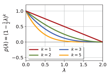
(a) Frequency response

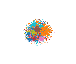
(b) Raw features

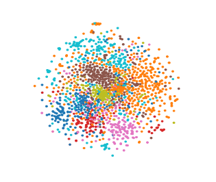
(c) $k=1$

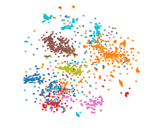
(d) $k=12$

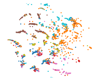
(e) $k=100$

Figure 1: (a) Frequency response functions. (b-e) t-SNE visualization of the raw and filtered node features of Cora with different $k$.

3.2 Graph Convolution

To formally define graph convolution, we first introduce the notions of graph signal and graph filter Shuman et al. (2013). A graph signal can be represented as a vector $\bm{f}=[f(v_{1}),\cdots,f(v_{n})]^{\top}$, where $f:\mathcal{V}\to\mathbb{R}$ is a real-valued function on the nodes of a graph. Given an adjacency matrix $A$ and the degree matrix $D=\text{diag}(d_{1},\cdots,d_{n})$, the symmetrically normalized graph Laplacian $L_{s}=I-D^{-\frac{1}{2}}AD^{-\frac{1}{2}}$ can be eigen-decomposed as $L_{s}=U\Lambda U^{-1}$, where $\Lambda=\text{diag}(\lambda_{1},\cdots,\lambda_{n})$ are the eigenvalues in increasing order, and $U=[\bm{u}_{1},\cdots,\bm{u}_{n}]$ are the associated orthogonal eigenvectors. A linear graph filter can be represented as a matrix $G=Up(\Lambda)U^{-1}\in\mathbb{R}^{n\times n}$, where $p(\Lambda)=\text{diag}(p(\lambda_{1}),\cdots,p(\lambda_{n}))$ is called the frequency response function of $G$. Graph convolution is defined as the multiplication of a graph signal $\bm{f}$ with a graph filter $G$:

$$\bar{\bm{f}}=G\bm{f},$$ (1)

where $\bar{\bm{f}}$ is the filtered graph signal.

Each column of the feature matrix $X$ can be considered as a graph signal. In graph signal processing Shuman et al. (2013), the eigenvalues $(\lambda_{q})_{1\leq q\leq n}$ can be taken as frequencies and the associated eigenvectors $(\bm{u}_{q})_{1\leq q\leq n}$ are considered as Fourier basis of the graph. A graph signal $\bm{f}$ can be decomposed into a linear combination of the eigenvectors, i.e.,

$$\bm{f}=U\bm{z}=\sum\nolimits_{q=1}^{n}{z_{q}\bm{u}_{q}},$$ (2)

where $\bm{z}=[z_{1},\cdots,z_{n}]^{\top}$ and $z_{q}$ is the coefficient of $\bm{u}_{q}$. The magnitude of the coefficient $|z_{q}|$ indicates the strength of the basis signal $\bm{u}_{q}$ presented in $\bm{f}$.

A graph signal is smooth if nearby nodes on the graph have similar features representations. The smoothness of a basis signal $\bm{u}_{q}$ can be measured by Laplacian-Beltrami operator $\Omega(\cdot)$ Chung and Graham (1997), i.e.,

$$\begin{split}\Omega(\bm{u}_{q})&=\frac{1}{2}\sum_{(v_{i},v_{j})\in\mathcal{E}}{a_{ij}\left\|\frac{\bm{u}_{q}(i)}{\sqrt{d_{i}}}-\frac{\bm{u}_{q}(j)}{\sqrt{d_{j}}}\right\|_{2}^{2}}\\ &={\bm{u}_{q}}^{\top}L_{s}{\bm{u}_{q}}=\lambda_{q},\end{split}$$ (3)

where $\bm{u}_{q}(i)$ denotes the $i$-th element of the vector $\bm{u}_{q}$. (3) indicates that the basis signals associated with lower frequencies (smaller eigenvalues) are smoother, which means that a smooth graph signal $\bm{f}$ should contain more low-frequency basis signals than high-frequency ones. This can be achieved by performing graph convolution with a low-pass graph filter $G$, as shown below.

By (2), the graph convolution can be written as

$$\bar{\bm{f}}=G\bm{f}=Up(\Lambda)U^{-1}\cdot U\bm{z}=\sum\nolimits_{q=1}^{n}{p(\lambda_{q})z_{q}\bm{u}_{q}}.$$ (4)

In the filtered signal $\bar{\bm{f}}$, the coefficient $z_{q}$ of the basis signal $\bm{u}_{q}$ is scaled by $p(\lambda_{q})$. To preserve the low-frequency basis signals and remove the high-frequency ones in $\bm{f}$, the graph filter $G$ should be low-pass, i.e., the frequency response function $p(\cdot)$ should be decreasing and nonnegative.

A low-pass graph filter can take on many forms. Here, we design a low-pass graph filter with the frequency response function

$$p(\lambda_{q})=1-\frac{1}{2}\lambda_{q}.$$ (5)

As shown by the red line in Figure 1(a), one can see that $p(\cdot)$ in (5) is decreasing and nonnegative on $[0,2]$. Note that all the eigenvalues $\lambda_{q}$ of the symmetrically normalized graph Laplacian $L_{s}$ fall into interval $[0,2]$ Chung and Graham (1997), which indicates that $p(\cdot)$ in (5) is low-pass. The graph filter $G$ with $p(\cdot)$ in (5) as the frequency response function can then be written as

$$G=Up(\Lambda)U^{-1}=U(I-\frac{1}{2}\Lambda)U^{-1}=I-\frac{1}{2}L_{s}.$$ (6)

By performing graph convolution on the feature matrix $X$, we obtain the filtered feature matrix:

$$\bar{X}=GX,$$ (7)

where $\bar{X}=[\bm{\bar{x}}_{1},\bm{\bar{x}}_{2},\cdots,\bm{\bar{x}}_{n}]^{\top}\in\mathbb{R}^{n\times d}$ is the filtered node features after graph convolution. Applying such a low-pass graph filter on the feature matrix makes adjacent nodes have similar feature values along each dimension, i.e., the graph signals are smooth. Based on the cluster assumption that nearby nodes are likely to be in the same cluster, performing graph convolution with a low-pass graph filter will make the downstream clustering task easier.

Note that the proposed graph filter in (6) is different from the graph filter used in GCN. The graph filter in GCN is $G=I-L_{s}$ with the frequency response function $p(\lambda_{q})=1-\lambda_{q}$ Li et al. (2019), which is clearly not low-pass as it is negative for $\lambda_{q}\in(1,2]$ .

3.2.1 $k$-Order Graph Convolution

To make clustering easy, it is desired that nodes of the same class should have similar feature representations after graph filtering. However, the first-order graph convolution in (7) may not be adequate to achieve this, especially for large and sparse graphs, as it updates each node $v_{i}$ by the aggregation of its $1$-hop neighbours only, without considering long-distance neighbourhood relations. To capture global graph structures and facilitate clustering, we propose to use $k$-order graph convolution.

We define $k$-order graph convolution as

$$\bar{X}=(I-\frac{1}{2}L_{s})^{k}X,$$ (8)

where $k$ is a positive integer, and the corresponding graph filter is

$$G=(I-\frac{1}{2}L_{s})^{k}=U(I-\frac{1}{2}\Lambda)^{k}U^{-1}.$$ (9)

The frequency response function of $G$ in (9) is

$$p(\lambda_{q})=(1-\frac{1}{2}\lambda_{q})^{k}.$$ (10)

As shown in Figure 1(a), $p(\lambda_{q})$ in (10) becomes more low-pass as $k$ increases, indicating that the filtered node features $\bar{X}$ will be smoother.

The iterative calculation formula of $k$-order graph convolution is

$$\begin{split}&\bm{\bar{x}}_{i}^{(0)}={\bm{x}_{i}},\quad\bm{\bar{x}}_{i}^{(1)}=\frac{1}{2}\left(\bm{\bar{x}}_{i}^{(0)}+\sum_{(v_{i},v_{j})\in\mathcal{E}}\frac{a_{ij}}{\sqrt{d_{i}d_{j}}}\bm{\bar{x}}_{j}^{(0)}\right),\cdots,\\ &\bm{\bar{x}}_{i}^{(k)}=\frac{1}{2}\left(\bm{\bar{x}}_{i}^{(k-1)}+\sum_{(v_{i},v_{j})\in\mathcal{E}}\frac{a_{ij}}{\sqrt{d_{i}d_{j}}}\bm{\bar{x}}_{j}^{(k-1)}\right),\end{split}$$ (11)

and the final $\bm{\bar{x}}_{i}$ is $\bm{\bar{x}}_{i}^{(k)}$.

From (11), one can easily see that $k$-order graph convolution updates the features of each node $v_{i}$ by aggregating the features of its $k$-hop neighbours iteratively. As $k$-order graph convolution takes into account long-distance data relations, it can be useful for capturing global graph structures to improve clustering performance.

3.2.2 Theoretical Analysis

As $k$ increases, $k$-order graph convolution will make the node features smoother on each dimension. In the following, we prove this using the Laplacian-Beltrami operator $\Omega(\cdot)$ defined in (3). Denote by $\bm{f}$ a column of the feature matrix $X$, which can be decomposed as $\bm{f}=U\bm{z}$. Note that $\Omega(\beta\bm{f})=\beta^{2}\Omega(\bm{f})$, where $\beta$ is a scalar. Therefore, to compare the smoothness of different graph signals, we need to put them on a common scale. In what follows, we consider the smoothness of a normalized signal $\frac{\bm{f}}{\lVert\bm{f}\rVert_{2}}$, i.e.,

$$\Omega\left(\frac{\bm{f}}{\lVert\bm{f}\rVert_{2}}\right)=\frac{\bm{f}^{\top}L_{s}\bm{f}}{\lVert\bm{f}\rVert_{2}^{2}}=\frac{\bm{z}^{\top}\Lambda\bm{z}}{\lVert\bm{z}\rVert_{2}^{2}}=\frac{\sum_{i=1}^{n}\lambda_{i}z_{i}^{2}}{\sum_{i=1}^{n}{z_{i}^{2}}}.$$ (12)

Theorem 1.

If the frequency response function $p(\lambda)$ of a graph filter $G$ is nonincreasing and nonnegative for all $\lambda_{i}$, then for any signal $\bm{f}$ and the filtered signal $\bar{\bm{f}}=G\bm{f}$, we always have

$$\Omega\left(\frac{\bar{\bm{f}}}{\lVert\bar{\bm{f}}\rVert_{2}}\right)\leq\Omega\left(\frac{\bm{f}}{\lVert\bm{f}\rVert_{2}}\right).$$

Proof.

We first prove the following lemma by induction. The following inequality

$$T_{c}^{(n)}=\frac{\sum_{i=1}^{n}c_{i}T_{i}}{\sum_{i=1}^{n}c_{i}}\leq\frac{\sum_{i=1}^{n}b_{i}T_{i}}{\sum_{i=1}^{n}b_{i}}=T_{b}^{(n)}$$ (13)

holds, if $T_{1}\leq\cdots\leq T_{n}$ and $\frac{c_{1}}{b_{1}}\geq\cdots\geq\frac{c_{n}}{b_{n}}$ with $\forall c_{i},b_{i}\geq 0$. It is easy to validate that it holds when $n=2$.

Now assume that it holds when $n=l-1$, i.e., $T_{c}^{(l-1)}\leq T_{b}^{(l-1)}$. Then, consider the case of $n=l$ and we have

$$\begin{split}\frac{\sum_{i=1}^{l}c_{i}T_{i}}{\sum_{i=1}^{l}c_{i}}&=\frac{\sum_{i=1}^{l-1}c_{i}T_{i}+c_{l}T_{l}}{\sum_{i=1}^{l-1}c_{i}+c_{l}}\\ &=\frac{(\sum_{i=1}^{l-1}{c_{i}})T_{c}^{(l-1)}+c_{l}T_{l}}{\sum_{i=1}^{l-1}c_{i}+c_{l}}\\ &\leq\frac{(\sum_{i=1}^{l-1}{c_{i}})T_{b}^{(l-1)}+c_{l}T_{l}}{\sum_{i=1}^{l-1}c_{i}+c_{l}}.\end{split}$$ (14)

Since $T_{b}^{(l-1)}=\frac{\sum_{i=1}^{l-1}b_{i}T_{i}}{\sum_{i=1}^{l-1}b_{i}}\leq\frac{\sum_{i=1}^{l-1}b_{i}T_{l-1}}{\sum_{i=1}^{l-1}b_{i}}=T_{l-1}$, we have $T_{b}^{(l-1)}\leq T_{l}$. Also note that $\frac{\sum_{i=1}^{l-1}c_{i}}{\sum_{i=1}^{l-1}b_{i}}\geq\frac{c_{l}}{b_{l}}$. Since the lemma holds when $n=2$, we have

$$\begin{split}\frac{(\sum_{i=1}^{l-1}{c_{i}})T_{b}^{(l-1)}+c_{l}T_{l}}{\sum_{i=1}^{l-1}c_{i}+c_{l}}&\leq\frac{(\sum_{i=1}^{l-1}{b_{i}})T_{b}^{(l-1)}+b_{l}T_{l}}{\sum_{i=1}^{l-1}b_{i}+b_{l}}\\ &=\frac{\sum_{i=1}^{l}b_{i}T_{i}}{\sum_{i=1}^{l}b_{i}},\end{split}$$ (15)

which shows that the inequality (13) also holds when $n=l$. By induction, the above lemma holds for all $n$.

We can now prove Theorem 1 using this lemma. For convenience, we arrange the eigenvalues $\lambda_{i}$ of $L_{s}$ in increasing order such that $0\leq\lambda_{1}\leq\cdots\leq\lambda_{n}$. Since $p(\lambda)$ is nonincreasing and nonnegative, $p(\lambda_{1})\geq\cdots\geq p(\lambda_{n})\geq 0$. Theorem 1 can then be proved with the above lemma by letting

$$T_{i}=\lambda_{i},\quad b_{i}=z_{i}^{2},\quad c_{i}=p^{2}(\lambda_{i})z_{i}^{2}.$$ (16)

∎

Assuming that $\bm{f}$ and $\bar{\bm{f}}$ are obtained by $(k-1)$-order and $k$-order graph convolution respectively, one can immediately infer from Theorem 1 that $\bar{\bm{f}}$ is smoother than $\bm{f}$. In other words, $k$-order graph convolution will produce smoother features as $k$ increases. Since nodes in the same cluster tend to be densely connected, they are likely to have more similar feature representations with large $k$, which can be beneficial for clustering.

3.3 Clustering via Adaptive Graph Convolution

We perform the classical spectral clustering method Perona and Freeman (1998); Von Luxburg (2007) on the filtered feature matrix $\bar{X}$ to partition the nodes of $\mathcal{V}$ into $m$ clusters, similar to Wang et al. (2017). Specifically, we first apply the linear kernel $K=\bar{X}\bar{X}^{T}$ to learn pairwise similarity between nodes, and then we calculate $W=\frac{1}{2}(|K|+|K^{\top}|)$ to make sure that the similarity matrix is symmetric and nonnegative, where $|\cdot|$ means taking absolute value of each element of the matrix. Finally, we perform spectral clustering on $W$ to obtain clustering results by computing the eigenvectors associated with the $m$ largest eigenvalues of $W$ and then applying the k-means algorithm on the eigenvectors to obtain cluster partitions.

The central issue of $k$-order graph convolution is how to select an appropriate $k$. Although $k$-order graph convolution can make nearby nodes have similar feature representations, $k$ is definitely not the larger the better. $k$ being too large will lead to over-smoothing, i.e., the features of nodes in different clusters are mixed and become indistinguishable. Figure 1(b-e) visualizes the raw and filtered node features of the Cora citation network with different $k$, where the features are projected by t-SNE Van der Maaten and Hinton (2008) and nodes of the same class are indicated by the same colour. It can be seen that the node features become similar as $k$ increases. The data exhibits clear cluster structures with $k=12$. However, with $k=100$, the features are over-smoothed and nodes from different clusters are mixed together.

To adaptively select the order $k$, we use the clustering performance metric – internal criteria based on the information intrinsic to the data alone Aggarwal and Reddy (2014). Here, we consider intra-cluster distance ($intra(\mathcal{C})$ for a given cluster partition $\mathcal{C}$), which represents the compactness of $\mathcal{C}$:

$$intra(\mathcal{C})=\frac{1}{|\mathcal{C}|}\sum_{C\in\mathcal{C}}\frac{1}{|C|(|C|-1)}\sum_{\begin{subarray}{c}v_{i},v_{j}\in C,\\ v_{i}\neq v_{j}\end{subarray}}\|\bar{x}_{i}-\bar{x}_{j}\|_{2}.$$ (17)

Note that inter-cluster distance can also be used to measure clustering performance given fixed data features, and a good cluster partition should have a large inter-cluster distance and a small intra-cluster distance. However, by Theorem 1, the node features become smoother as $k$ increases, which could significantly reduce both intra-cluster and inter-cluster distances. Hence, inter-cluster distance may not be a reliable metric for measuring the clustering performance w.r.t. different $k$, and so we propose to observe the variation of intra-cluster distance for choosing $k$.

Our strategy is to find the first local minimum of $intra(\mathcal{C})$ w.r.t. $k$. Specifically, we start from $k=1$ and increment it by 1 iteratively. In each iteration $t$, we first obtain the cluster partition $\mathcal{C}^{(t)}$ by performing $k$-order ($k=t$) graph convolution and spectral clustering, then we compute $intra(\mathcal{C}^{(t)})$. Once $intra(\mathcal{C}^{(t)})$ is larger than $intra(\mathcal{C}^{(t-1)})$, we stop the iteration and set the chosen $k=t-1$. More formally, consider $d\_intra(t-1)=intra(\mathcal{C}^{(t)})-intra(\mathcal{C}^{(t-1)})$, the criterion for stopping the iteration is $d\_intra(t-1)>0$, i.e., stops at the first local minimum of $intra(\mathcal{C}^{(t)})$. So, the final choice of cluster partition is $\mathcal{C}^{(t-1)}$. The benefits of this selection strategy are two-fold. First, it ensures finding a local minimum for $intra(\mathcal{C})$ that may indicate a good cluster partition and avoids over-smoothing. Second, it is time efficient to stop at the first local minimum of $intra(\mathcal{C})$.

3.4 Algorithm Procedure and Time Complexity

Algorithm 1 AGC

0:  Node set $\mathcal{V}$, adjacency matrix $A$, feature matrix $X$, and maximum iteration number $max\_iter$.

0:  Cluster partition $\mathcal{C}$.

1:  Initialize $t=0$ and $intra(\mathcal{C}^{(0)})=+\infty$. Compute the symmetrically normalized graph Laplacian $L_{s}=I-D^{-\frac{1}{2}}AD^{-\frac{1}{2}}$, where $D$ is the degree matrix of $A$.

2:  repeat

3:     Set $t=t+1$ and $k=t$.

4:     Perform $k$-order graph convolution by Eq. (8) and get $\bar{X}$.

5:     Apply the linear kernel $K=\bar{X}\bar{X}^{T}$, and calculate the similarity matrix $W=\frac{1}{2}(|K|+|K^{T}|)$.

6:     Obtain the cluster partition $\mathcal{C}^{(t)}$ by performing spectral clustering on $W$.

7:     Compute $intra(\mathcal{C}^{(t)})$ by Eq. (17).

8:  until $d\_intra(t-1)>0$ or $t>max\_iter$

9:  Set $k=t-1$ and $\mathcal{C}=\mathcal{C}^{(t-1)}$.

The overall procedure of AGC is shown in Algorithm 1. Denote by $n$ the number of nodes, $d$ the number of attributes, $m$ the number of clusters, and $N$ the number of nonzero entries of the adjacency matrix $A$. Note that for a sparse $A$, $N<<n^{2}$. The time complexity of computing $L_{s}$ in the initialization is $\mathcal{O}(N)$. In each iteration, for a sparse $L_{s}$, the fastest way of computing $k$-order graph convolution in (8) is to left multiply $X$ by $I-\frac{1}{2}L_{s}$ repeatedly for $k$ times, which has the time complexity $\mathcal{O}(Ndk)$. The time complexity of performing spectral clustering on $\bar{X}$ in each iteration is $\mathcal{O}(n^{2}d+n^{2}m)$. The time complexity of computing $intra(\mathcal{C})$ in each iteration is $\mathcal{O}(\frac{1}{m}n^{2}d)$. Since $m$ is usually much smaller than $n$ and $d$, the time complexity of each iteration is approximately $\mathcal{O}(n^{2}d+Ndk)$. If Algorithm 1 iterates $t$ times, the overall time complexity of AGC is $\mathcal{O}(n^{2}dt+Ndt^{2})$. Unlike existing GCN based clustering methods, AGC does not need to train the neural network parameters, which makes it time efficient.

4 Experiments

4.1 Datasets

We evaluate our method AGC on four benchmark attributed networks. Cora, Citeseer and Pubmed Kipf and Welling (2016) are citation networks where nodes correspond to publications and are connected if one cites the other. Wiki Yang et al. (2015) is a webpage network where nodes are webpages and are connected if one links the other. The nodes in Cora and Citeseer are associated with binary word vectors, and the nodes in Pubmed and Wiki are associated with tf-idf weighted word vectors. Table 1 summarizes the details of the datasets.

Dataset	#Nodes	#Edges	#Features	#Classes
Cora	2708	5429	1433	7
Citeseer	3327	4732	3703	6
Pubmed	19717	44338	500	3
Wiki	2405	17981	4973	17

Table 1: Dataset statistics.

Methods	Input	Cora			Citeseer			Pubmed			Wiki
		Acc%	NMI%	F1%	Acc%	NMI%	F1%	Acc%	NMI%	F1%	Acc%	NMI%	F1%
k-means	Feature	34.65	16.73	25.42	38.49	17.02	30.47	57.32	29.12	57.35	33.37	30.20	24.51
Spectral-f	Feature	36.26	15.09	25.64	46.23	21.19	33.70	59.91	32.55	58.61	41.28	43.99	25.20
Spectral-g	Graph	34.19	19.49	30.17	25.91	11.84	29.48	39.74	3.46	51.97	23.58	19.28	17.21
DeepWalk	Graph	46.74	31.75	38.06	36.15	9.66	26.70	61.86	16.71	47.06	38.46	32.38	25.74
DNGR	Graph	49.24	37.29	37.29	32.59	18.02	44.19	45.35	15.38	17.90	37.58	35.85	25.38
GAE	Both	53.25	40.69	41.97	41.26	18.34	29.13	64.08	22.97	49.26	17.33	11.93	15.35
VGAE	Both	55.95	38.45	41.50	44.38	22.71	31.88	65.48	25.09	50.95	28.67	30.28	20.49
MGAE	Both	63.43	45.57	38.01	63.56	39.75	39.49	43.88	8.16	41.98	50.14	47.97	39.20
ARGE	Both	64.00	44.90	61.90	57.30	35.00	54.60	59.12	23.17	58.41	41.40	39.50	38.27
ARVGE	Both	63.80	45.00	62.70	54.40	26.10	52.90	58.22	20.62	23.04	41.55	40.01	37.80
AGC	Both	68.92	53.68	65.61	67.00	41.13	62.48	69.78	31.59	68.72	47.65	45.28	40.36

Table 2: Clustering performance.

4.2 Baselines and Evaluation Metrics

We compare AGC with three kinds of clustering methods. 1) Methods that only use node features: k-means and spectral clustering (Spectral-f) that constructs a similarity matrix with the node features by linear kernel. 2) Structural clustering methods that only use graph structures: spectral clustering (Spectral-g) that takes the node adjacency matrix as the similarity matrix, DeepWalk Perozzi et al. (2014), and deep neural networks for graph representations (DNGR) Cao et al. (2016). 3) Attributed graph clustering methods that utilize both node features and graph structures: graph autoencoder (GAE) and graph variational autoencoder (VGAE) Kipf and Welling (2016), marginalized graph autoencoder (MGAE) Wang et al. (2017), and adversarially regularized graph autoencoder (ARGE) and variational graph autoencoder (ARVGE) Pan et al. (2018).

To evaluate the clustering performance, we adopt three widely used performance measures Aggarwal and Reddy (2014): clustering accuracy (Acc), normalized mutual information (NMI), and macro F1-score (F1).

4.3 Parameter Settings

For AGC, we set $max\_iter=60$. For other baselines, we follow the parameter settings in the original papers. In particular, for DeepWalk, the number of random walks is 10, the number of latent dimensions for each node is 128, and the path length of each random walk is 80. For DNGR, the autoencoder is of three layers with 512 neurons and 256 neurons in the hidden layers respectively. For GAE and VGAE, we construct encoders with a 32-neuron hidden layer and a 16-neuron embedding layer, and train the encoders for 200 iterations using the Adam optimizer with learning rate 0.01. For MGAE, the corruption level $p$ is 0.4, the number of layers is 3, and the parameter $\lambda$ is $10^{-5}$. For ARGE and ARVGE, we construct encoders with a 32-neuron hidden layer and a 16-neuron embedding layer. The discriminators are built by two hidden layers with 16 neurons and 64 neurons respectively. On Cora, Citeseer and Wiki, we train the autoencoder-related models of ARGE and ARVGE for 200 iterations with the Adam optimizer, with the encoder learning rate and the discriminator learning rate both as 0.001; on Pubmed, we train them for 2000 iterations with the encoder learning rate 0.001 and the discriminator learning rate 0.008.

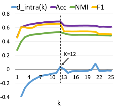
(a) Cora

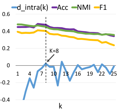
(b) Wiki

Figure 2: $d\_intra(k)$ and clustering performance w.r.t. $k$.

4.4 Result Analysis

We run each method 10 times for each dataset and report the average clustering results in Table 2, where the top 2 results are highlighted in bold. The observations are as follows.

1) AGC consistently outperforms the clustering methods that only exploit either node features or graph structures by a very large margin, due to the clear reason that AGC makes a better use of available data by integrating both kinds of information, which can complement each other and greatly improve clustering performance.

2) AGC consistently outperforms existing attributed graph clustering methods that use both node features and graph structures. This is because AGC can better utilize graph information than these methods. In particular, GAE, VGAE, ARGE and ARVGE only exploit 2-hop neighbourhood of each node to aggregate information, and MGAE only exploits 3-hop neighbourhood. In contrast, AGC uses $k$-order graph convolution with an automatically selected $k$ to aggregate information within $k$-hop neighbourhood to produce better feature representations for clustering.

3) AGC outperforms the strongest baseline MGAE by a considerable margin on Cora, Citeseer and Pubmed, and is comparable to MGAE on Wiki. This is probably because Wiki is more densely connected than others and aggregating information within 3-hop neighbourhood may be enough for feature smoothing. But it is not good enough for larger and sparser networks such as Citeseer and Pubmed, on which the performance gaps between AGC and MGAE are wider. AGC deals with the diversity of networks well via adaptively selecting a good $k$ for different networks.

To demonstrate the validity of the proposed selection criterion $d\_intra(t-1)>0$, we plot $d\_intra(k)$ and the clustering performance w.r.t. $k$ on Cora and Wiki respectively in Figure 2. The curves of Citeseer and Pubmed are not plotted due to space limitations. One can see that when $d\_intra(k)>0$, the corresponding Acc, NMI and F1 values are the best or close to the best, and the clustering performance declines afterwards. It shows that the selection criterion can reliably find a good cluster partition and prevent over-smoothing. The selected $k$ for Cora, Citeseer, Pubmed and Wiki are 12, 55, 60, and 8 respectively, which are close to the best $k\in[0,60]$ – 12, 35, 60, and 6 on these datasets respectively, demonstrating the effectiveness of the proposed selection criterion.

AGC is quite stable. The standard deviations of Acc, NMI and F1 are 0.17%, 0.42%, 0.01% on Cora, 0.24%, 0.36%, 0.19% on Citeseer, 0.00%, 0.00%, 0.00% on Pubmed, and 0.79%, 0.17%, 0.20% on Wiki, all very small.

The running time of AGC (in Python, with NVIDIA Geforce GTX 1060 6GB GPU) on Cora, Citeseer, Pubmed and Wiki is 5.78, 62.06, 584.87, and 10.75 seconds respectively. AGC is a little slower than GAE, VGAE, ARGE and ARVGE on Citeseer, but is more than twice faster on the other three datasets. This is because AGC does not need to train the neural network parameters as in these methods, and hence is more time efficient even with a relatively large $k$.

5 Conclusion

In this paper, we propose a simple and effective method for attributed graph clustering. To make a better use of available data and capture global cluster structures, we design a $k$-order graph convolution to aggregate long-range data information. To optimize clustering performance on different graphs, we design a strategy for adaptively selecting an appropriate $k$. This enables our method to achieve competitive performance compared to classical and state-of-the-art methods. In future work, we plan to improve the adaptive selection strategy to make our method more robust and efficient.

References

- Aggarwal and Reddy [2014] Charu C Aggarwal and Chandan K Reddy. Data Clustering: Algorithms and Applications. CRC Press, Boca Raton, 2014.
- Bojchevski and Günnemann [2018] Aleksandar Bojchevski and Stephan Günnemann. Bayesian robust attributed graph clustering: Joint learning of partial anomalies and group structure. In AAAI, 2018.
- Cai et al. [2018] HongYun Cai, Vincent W. Zheng, and Kevin Chen-Chuan Chang. A comprehensive survey of graph embedding: Problems, techniques, and applications. TKDE, 30(9):1616–1637, 2018.
- Cao et al. [2015] Shaosheng Cao, Wei Lu, and Qiongkai Xu. Grarep: Learning graph representations with global structural information. In CIKM, pages 891–900, 2015.
- Cao et al. [2016] Shaosheng Cao, Wei Lu, and Qiongkai Xu. Deep neural networks for learning graph representations. In AAAI, pages 1145–1152, 2016.
- Chang and Blei [2009] Jonathan Chang and David Blei. Relational topic models for document networks. In Artificial Intelligence and Statistics, pages 81–88, 2009.
- Chung and Graham [1997] Fan RK Chung and Fan Chung Graham. Spectral graph theory. Number 92. American Mathematical Society, 1997.
- Grover and Leskovec [2016] Aditya Grover and Jure Leskovec. node2vec: Scalable feature learning for networks. In KDD, pages 855–864, 2016.
- He et al. [2017] Dongxiao He, Zhiyong Feng, Di Jin, Xiaobao Wang, and Weixiong Zhang. Joint identification of network communities and semantics via integrative modeling of network topologies and node contents. In AAAI, pages 116–124, 2017.
- Kipf and Welling [2016] Thomas N Kipf and Max Welling. Variational graph auto-encoders. NIPS Workshop on Bayesian Deep Learning, 2016.
- Kipf and Welling [2017] Thomas N Kipf and Max Welling. Semi-supervised classification with graph convolutional networks. In ICLR, 2017.
- Li et al. [2018] Ye Li, Chaofeng Sha, Xin Huang, and Yanchun Zhang. Community detection in attributed graphs: an embedding approach. In AAAI, pages 338–345, 2018.
- Li et al. [2019] Qimai Li, Xiao-Ming Wu, Han Liu, Xiaotong Zhang, and Zhichao Guan. Label efficient semi-supervised learning via graph filtering. CoRR, abs/1901.09993, 2019.
- Newman [2006] Mark EJ Newman. Finding community structure in networks using the eigenvectors of matrices. Physical Review E, 74(3):036104, 2006.
- Nikolentzos et al. [2017] Giannis Nikolentzos, Polykarpos Meladianos, and Michalis Vazirgiannis. Matching node embeddings for graph similarity. In AAAI, pages 2429–2435, 2017.
- Pan et al. [2018] Shirui Pan, Ruiqi Hu, Guodong Long, Jing Jiang, Lina Yao, and Chengqi Zhang. Adversarially regularized graph autoencoder for graph embedding. In IJCAI, pages 2609–2615, 2018.
- Perona and Freeman [1998] Pietro Perona and William Freeman. A factorization approach to grouping. In ECCV, pages 655–670, 1998.
- Perozzi et al. [2014] Bryan Perozzi, Rami Al-Rfou, and Steven Skiena. Deepwalk: Online learning of social representations. In KDD, pages 701–710, 2014.
- Schaeffer [2007] Satu Elisa Schaeffer. Graph clustering. Computer Science Review, 1(1):27–64, 2007.
- Shuman et al. [2013] David I Shuman, Sunil K Narang, Pascal Frossard, Antonio Ortega, and Pierre Vandergheynst. The emerging field of signal processing on graphs: Extending high-dimensional data analysis to networks and other irregular domains. IEEE Signal Processing Magazine, 30(3):83–98, 2013.
- Van der Maaten and Hinton [2008] L.J.P. Van der Maaten and G.E. Hinton. Visualizing high-dimensional data using t-SNE. Journal of Machine Learning Research, 9:2579–2605, 2008.
- Von Luxburg [2007] Ulrike Von Luxburg. A tutorial on spectral clustering. Statistics and Computing, 17(4):395–416, 2007.
- Wang et al. [2016a] Daixin Wang, Peng Cui, and Wenwu Zhu. Structural deep network embedding. In KDD, pages 1225–1234, 2016.
- Wang et al. [2016b] Xiao Wang, Di Jin, Xiaochun Cao, Liang Yang, and Weixiong Zhang. Semantic community identification in large attribute networks. In AAAI, pages 265–271, 2016.
- Wang et al. [2017] Chun Wang, Shirui Pan, Guodong Long, Xingquan Zhu, and Jing Jiang. Mgae: Marginalized graph autoencoder for graph clustering. In CIKM, pages 889–898, 2017.
- Xia et al. [2014] Rongkai Xia, Yan Pan, Lei Du, and Jian Yin. Robust multi-view spectral clustering via low-rank and sparse decomposition. In AAAI, pages 2149–2155, 2014.
- Yang et al. [2009] Tianbao Yang, Rong Jin, Yun Chi, and Shenghuo Zhu. Combining link and content for community detection: a discriminative approach. In KDD, pages 927–936, 2009.
- Yang et al. [2013] Jaewon Yang, Julian McAuley, and Jure Leskovec. Community detection in networks with node attributes. In ICDM, pages 1151–1156, 2013.
- Yang et al. [2015] Cheng Yang, Zhiyuan Liu, Deli Zhao, Maosong Sun, and Edward Y Chang. Network representation learning with rich text information. In IJCAI, pages 2111–2117, 2015.
- Ye et al. [2018] Fanghua Ye, Chuan Chen, and Zibin Zheng. Deep autoencoder-like nonnegative matrix factorization for community detection. In CIKM, pages 1393–1402, 2018.