MASS-LOSS RATES FOR O AND EARLY B STARS POWERING BOWSHOCK NEBULAE: EVIDENCE FOR BI-STABILITY BEHAVIOR

Abstract

Second only to initial mass, the rate of wind-driven mass loss determines the final mass of a massive star and the nature of its remnant. Motivated by the need to reconcile observational values and theory, we use a recently vetted technique to analyze the mass-loss rates in a sample of OB stars that generate bowshock nebulae. We measure peculiar velocities from new $Gaia$ parallax and proper motion data and their spectral types from new optical and infrared spectroscopy. For our sample of 70 central stars in morphologically selected bowshocks nebulae, 67 are OB stars. The median peculiar velocity is 11 km s^-1, significantly smaller than classical “runaway star” velocities. Mass-loss rates for these O and early B stars agree with recently lowered theoretical predictions, ranging from $\simeq$10^-7 $M_{\odot}$ yr^-1 for mid-O dwarfs to 10^-9 $M_{\odot}$ yr^-1  for late-O dwarfs—a factor of about 2.7 lower than the often-used Vink et al. (2001) formulation. Our results provide the first observational mass-loss rates for B0–B3 dwarfs and giants—10^-9 to 10^-8 $M_{\odot}$ yr^-1. We find evidence for an increase in the mass-loss rates below a critical effective temperature, consistent with predictions of the bi-stability phenomenon in the range $T_{\rm eff}$=19,000–27,000 K. The sample exhibits a correlation between modified wind momentum and luminosity, consistent in slope but lower by 0.43 dex in magnitude compared to canonical wind-luminosity relations. We identify a small subset of objects deviating most significantly from theoretical expectations as probable radiation-driven bow wave nebulae by virtue of their low stellar-to-nebular luminosity ratios. For these, the inferred mass-loss rates must be regarded as upper limits.

1 Introduction

The rate at which massive stars expel material in radiation-driven winds is a fundamental factor in their evolution. Large mass-loss rates reduce final core masses and, thereby, determine the type of supernova that ensues, as well as the nature of the final compact object (e.g., white dwarf, neutron star, black hole, or none). For the $\simeq$50% of massive stars that have close companions (Kobulnicky & Fryer, 2007; Sana et al., 2012; Kobulnicky et al., 2016), mass exchange and common envelope evolution may become the overriding evolutionary influences. But for single massive stars, stars with distant companions (effectively single), and even in close binaries prior to interaction, wind mass loss removes copious amounts of envelope material on timescales relevant to the rapid evolution of such stars. Measured mass-loss rates, $\dot{M}$, lie in the range $<$10^-9 to few $\times$ 10^-6 $M_{\odot}$ yr^-1, depending on stellar mass and evolutionary stage (e.g., Garmany et al., 1981; Howarth & Prinja, 1989; Fullerton et al., 2006; Mokiem et al., 2007; Marcolino et al., 2009; Prinja & Massa, 2010). Kudritzki & Puls (2000), Puls et al. (2008), and Smith (2014) provide comprehensive reviews of massive star winds and mass loss.

Measurements of mass-loss rates at any given spectral type and luminosity class span orders of magnitude. H$\alpha$, radio continuum, and infrared observations measure the excess above the stellar photosphere and constitute the class of “$n^{2}$” diagnostics, since the extra-photospheric flux scales as the square of the density of material in the wind for optically thin geometries. This class of techniques typically yields mass-loss rates at the upper end of the range and larger than those predicted by theory unless corrected for the effects of “clumping”—density inhomogeneities in the wind (e.g., see Owocki et al., 1988; Leitherer, 1988; Fullerton et al., 1996; Martins et al., 2005b; Puls et al., 1996, 2005; Massa et al., 2017, for discussions of rates and clumping). The other canonical approach, ultraviolet absorption spectroscopy of high-ionization wind lines, typically yields mass-loss rates at the low end of the range and far below many theoretical models (Garmany et al., 1981; Howarth & Prinja, 1989; Fullerton et al., 2006; Marcolino et al., 2009). The former techniques become insensitive below rates of about 10^-7 $M_{\odot}$ yr^-1(Markova et al., 2004; Mokiem et al., 2007; Marcolino et al., 2009) while the latter becomes insensitive above 10^-7 $M_{\odot}$ yr^-1 as many UV resonance lines become saturated. In the limit of weak winds ($\dot{M}\lesssim 10^{-8}$ $M_{\odot}$ yr^-1, $\log(L/L_{\odot})\lesssim 5.2$), UV-based mass-loss rates fall two orders of magnitude below theoretical expectations. This “weak-wind problem” (Martins et al., 2005b; Mokiem et al., 2007; Marcolino et al., 2009; Muijres et al., 2012), coupled with the limitations of the canonical mass-loss techniques, especially for a whole range of stars later than about O7V, call for new approaches to diagnosing stellar mass loss. Promising techniques include X-ray (Cohen et al., 2014) or infrared (Najarro et al., 2011) spectroscopy of stellar winds.

A related unsolved problem in stellar winds is the impact of the “bi-stability” jump, characterized by a sudden increase in Lyman continuum and metal line opacity over a narrow temperature range predicted variously to lie somewhere between 19,000 K and 27,000 K (Pauldrach & Puls, 1990; Lamers et al., 1995; Vink et al., 2000; Petrov et al., 2016), with modern estimates falling at the low end of this range. This elevated opacity should produce a dramatic increase in mass-loss rate by factors of three to as much as 20 and a corresponding decrease in the terminal wind velocity. Observational verification of this putative bi-stable behavior is very limited. Markova & Puls (2008) observed a small sample of B supergiants on either side of the proposed bi-stability region and concluded that $\dot{M}$ increases only by factors of a few, if at all. Circumstantial evidence for larger enhancements in $\dot{M}$ comes from the slow rotation rates observed among B supergiants on the cool side of the bi-stability jump, interpreted as evidence for rotational braking through mass loss (bi-stability braking, Vink et al., 2010). Our study provides new data on mass-loss rates that will have implications for the effects of bi-stable behavior in stellar winds.

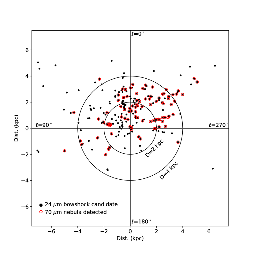
Figure 3: Distribution of 231 bowshock candidate stars having parallax:uncertainty ratios greater than 3:1 on the Galactic plane. The Sun’s location is at the center of the Figure. Red circles denote the subset of 94 that have 70 $\mu$m photometry from $HSO$. In this work we retain for analysis the 70 of these 94 that have measured spectral types.

In Kobulnicky et al. (2018) we refined an underexploited mass-loss measurement strategy, building upon a principle outlined in Kobulnicky et al. (2010) and first proposed by Gull & Sofia (1979). The approach entails the physical principle of momentum flux balance between a highly supersonic stellar wind and the impinging interstellar medium around a high-velocity “runaway” (Blaauw, 1961; Gies & Bolton, 1986) star. Along the surface where the momentum fluxes equate an arc-shaped shock (bowshock) forms (Wilkin, 1996, 2000) that may be detectable in the infrared continuum or emission lines (e.g., O III, H$\alpha$). While only about 15% of runaway stars have detectable infrared bowshock nebulae (Peri et al., 2015), over 700 candidate bowshocks around probable early type stars are known (Kobulnicky et al., 2016). Kobulnicky et al. (2018) estimated interstellar densities preceding bowshocks and suggested that ambient number densities exceeding 5 cm^-3 may be required to produce a detectable infrared bowshock nebula. This may explain why the Galactic latitude scale height of bowshock candidates (0.6 degrees; Kobulnicky et al., 2016, Figure 3) matches that of the molecular gas in the Milky Way. Identified most commonly by their 24 $\mu$m morphologies, the majority of arcuate nebulae also have corresponding 70 $\mu$m nebulae (Kobulnicky et al., 2017).

The mass-loss rates for such stars may be expressed in terms of quantities that are, in principle, observable:

$$\dot{M}={{4\pi R_{\rm 0}^{2}V_{\rm a}^{2}\rho_{\rm a}}\over{V_{\rm w}}}.$$ (1)

$R_{\rm 0}$ is the “standoff distance” between the star and the bowshock nebula, computed from an angular size on infrared images and a known distance. $V_{\rm w}$ is the terminal stellar wind speed, typically adopted from the literature according to the spectral type and luminosity class. $V_{\rm a}$ is the velocity of the star relative to the local interstellar medium (ISM), which may be computed from distance, proper motion, and radial velocity data in conjunction with a Galactic rotation curve model. Finally, $\rho_{\rm a}$ is the density of the ambient ISM, which Kobulnicky et al. (2018) estimated from the 70 $\mu$m infrared surface brightness using Draine & Li (2007, DL07) dust emission coefficients and assuming pre-shock/post-shock density ratio of 1:4 appropriate to strong shocks. In convenient astrophysical units the mass-loss rate may be expressed as,

$$\dot{M}(M_{\odot}~{}yr^{-1})=1.67\times 10^{-28}{{{[R_{\rm 0}{\rm(arcsec)}]^{2}}D{\rm(kpc)}~{}[V_{\rm a}{\rm(km~{}s^{-1})}]^{2}~{}I_{\nu}{\rm(Jy~{}sr^{-1})}}\over{V_{\rm w}{\rm(km~{}s^{-1})}~{}\ell{\rm(arcsec)}~{}j_{\nu}{\rm(Jy~{}cm^{2}~{}sr^{-1}~{}nucleon^{-1})}}}.$$ (2)

Here, $j_{\nu}$ is the frequency-dependent dust emission coefficient per nucleon as a function of ambient radiant energy density parameter from the star’s illuminating flux at the distance of the infrared nebula, $U$. $U$, in turn, may be obtained by knowing the standoff distance, the stellar luminosity from its effective temperature and radius, since the central star dominates the local radiation field by factors of 100 or more (Kobulnicky et al., 2017).

Finally, $I_{\nu}$ is the observed infrared suface brightness at the corresponding frequency. We use the surface brightnesses and scaled DL07 dust emission coefficients at 70 $\mu$m owing to the availability of Herschel Space Observatory ($HSO$) measurements in that band, but other wavelengths may eventually be proven suitable. We avoid using the 24 $\mu$m $Spitzer~{}Space~{}Telescope$ ($SST$) or 22 $\mu$m Wide-Field Infrared Survey Experiment ($WISE$) bandpasses because of the likelihood that this wavelength regime may be dominated by a population of stochasitically heated very small grains (Draine & Li, 2007). The path length through the nebulae is given by the observed angular chord diameter, $\ell$. $D$ is the distance to the star and nebula.

Our approach has the distinction of being rooted in a fundamentally different principle from other mass-loss measurement techniques. As such, we expect it to be insensitive to some of the uncertainties that limit other methods. Because the bowshocks typically lie several tenths of a parsec from the star, small-scale effects of wind clumping or temporal fluctuations in wind speed or density should be minimized through spatial and temporal averaging. At the same time, our technique is subject to its own set of assumptions and approximations.

• We assume isotropic stellar winds. But mass loss could be enhanced along the polar axis or reduced at the equatorial plane for rapidly rotating stars (Owocki et al., 1996; Langer, 1998; Müller & Vink, 2014).

• We assume a homogeneous interstellar medium. This is appropriate, on average, but certain to be incorrect for many real astrophysical examples.

• Our approach assumes that the velocity of the impinging ISM is directed radially in the frame of the star. Bulk flows of interstellar material at oblique angles relative to a moving star have been considered theoretically (Wilkin, 2000) and should produce asymmetric bowshock nebulae with morphologies similar to some of those cataloged in Kobulnicky et al. (2016). Such complications are beyond the scope of this effort.

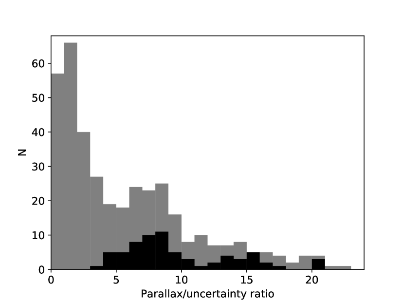
Figure 4: Histogram (gray) of the ratio parallax/uncertainty for the 394 candidate bowshock stars with entries in the GDR2. The black histogram shows the 70 stars retained for further analysis. These have known spectral types, 70 $\mu$m detections, and at least a 3:1 parallax:uncertainty ratio.

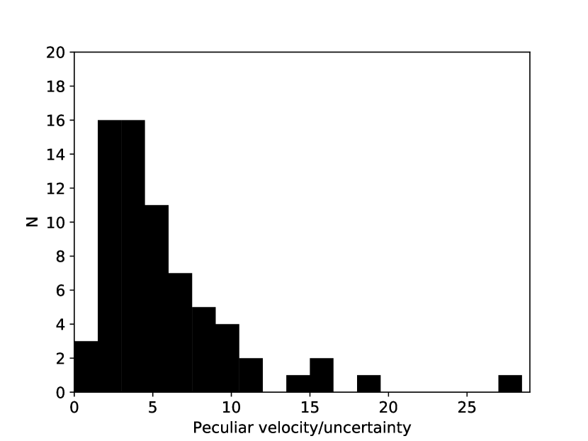
Figure 7: Histogram of the ratio peculiar velocity:uncertainty. The histogram depicts the 70  stars selected for analysis.

• The 1:4 pre/post-shock density ratio we adopt to estimate the interstellar density preceding the shock is merely a physically motivated assumption appropriate to strong non-radiative shocks. Density ratios in regions that experience significant cooling in radiative shocks could be more extreme. Hydrodynamical simulations of OB star bowshocks show that density ratios may reach factors of 10 over small scales that are well below the observational resolution limits. Factors of four are about right when averaged over $\simeq$0.1–0.3 pc scales typical of sample objects (e.g., Figures 7 and 4, respectively, of Comeron & Kaper, 1998; Meyer et al., 2017).

• It should be remembered that the measured geometrical quantities such as $R_{0}$ are projected quantities only. We apply a statistical correction factor of 1/sin(65°)$=$1.10 for inclination effects when computing $R_{0}$ in pc. This is a suitable correction because inclinations substantially smaller than about 50° would begin to mask the arcuate morphology and make the object unlikely to be included in the list of bowshock candidates (e.g., see Acreman et al. (2016) for numerical simulations of bowshocks at various inclination angles.) Given the large variation in signal-to-noise ratios of infrared images, we have not attempted to derive inclination angles for each object using geometrical properties of the nebulae (e.g., Tarango-Yong & Henney, 2018).

• We assume that the DL07 dust emission coefficients are appropriate to bowshock nebulae where a combination of radiative and shock heating may exist. In Section 2.2 we describe a rescaling of these coefficients made necessary by the harder radiation field of early type stars comapred to the interstellar radiation field. These dust models are constructed for dust that is radiatively heated. Kobulnicky et al. (2017) found that the dust color temperatures of bowshock nebulae were systematically above those expected from steady-state radiative heating from the central stars, leading them to propose this difference as evidence for shock heating, although this signature could also result from stochastically heated grains (A. Li, private communication). Additional heating by shocks could elevate dust emission coefficients beyond those adopted here. If shock heating is present but not properly accounted for, the adopted dust emission coefficients could be too small and the resulting mass-loss rates too large (c.f., Equation 2). To the contrary, Henney & Arthur (2019) argues that stellar wind particles do not propogate across the termination shock into the swept-up dusty region of the nebulae, and so shock heating is negligible.

Kobulnicky et al. (2018) employed the principle of momentum-balance for 20 bowshock-generating OB stars with known distances. They found stellar mass-loss rates factors of 10 or more lower than canonical $n^{2}$ diagnostics for a homogeneous wind, factors of 10 greater than UV absorption-line determinations, and factors of $\approx$2 lower than recent theoretical mass loss predictions (Vink et al., 2001; Lucy, 2010b). They concluded that, once corrected for geometrical clumping and porosity in velocity space, theoretical models would produce $\dot{M}$ predictions consistent with the bowshock method measurements. They further noted that the technique showed promise for measuring mass-loss rates for weak-winded late-O and early B stars, but there were not enough B stars in their sample to draw meaningful conclusions. Furthermore, uncertainties on the Kobulnicky et al. (2018) mass-loss rates were large and dominated by uncertainties on the stellar velocities (assumed there to be 30 km s^-1 for lack of direct measurement) and uncertainties on the distances to the stars. Because $\dot{M}$ in Equation 2 scales as the square of both $V_{\rm a}$ and $D$ in this technique ($D$, via the distance dependence implicit within the derived $U$ parameter on which dust emission coefficients are based), their results were highly sensitive to errors on these quantities.

With the availability of the $Gaia$ mission Data Release 2 (GDR2) data products (Gaia Collaboration et al., 2018), excellent parallaxes and proper motions—therefore, distances and peculiar velocities—are now available for an enlarged sample of bowshock-generating stars. In Kobulnicky et al. (2016) we compiled an “all-sky” catalog of 709 bowshock candidates consisting of arcuate infrared nebulae enclosing symmetrically placed stars. In Kobulnicky et al. (2017) we presented mid-IR photometry for the catalog of 709 bowshock candidates using archival $SST$, $WISE$, and $HSO$ images. In this contribution we extend the proof-of-concept sample of Kobulnicky et al. (2018) to measure mass-loss rates for stars having well-measured distances, velocities, and infrared bowshock properties. This expanded sample includes a greater fraction of early B stars and represents the first attempt at mass-loss determinations for dwarfs in this stellar temperature and luminosity regime. Section 2 describes the selection of sample targets and computation of requisite parameters. Section 3 details the section of the sample of stars for analysis. Section 4 presents the mass-loss rates with a comparison to previous literature results and theoretical model predictions. Section 5 summarizes the implications for mass loss prescriptions and for the evolution of massive stars.

2 New Data

2.1 Infrared and Optical Spectra from the Apache Point Observatory

We acquired new optical spectra of 15 candidate bowshock stars using the Double Imaging Spectrograph (DIS) at the Apache Point Observatory (APO) 3.5-meter telescope on the nights of 2018 May 12, May 19, and June 13. The 1200 line mm^-1 gratings in both the red and blue arms of the spectrograph yielded reciprocal dispersions of 0.58 and 0.62 Å pix ^-1, respectively, over wavelength ranges 5700–6900 Å and 4200–5500 Å, respectively. Exposure times ranged from 2$\times$300 s to several$\times$600 s depending on source magnitude, yielding spectra with signal-to-noise ratios (SNR) between 30:1 and 100:1 at 5900 Å. Seeing ranged between 1$\farcs$6 and 4$\farcs$0 in a 1$\farcs$5 $\times$110″ slit aligned at the parallactic angle, owing to the large airmass for the southern targets. The instrument HeNeAr lamps supplied periodic wavelength calibration to an RMS of 0.006 Å in the red channel and 0.1 Å in the blue channel. Instrument rotation produces wavelength shifts of up to 0.3 pix during the night which were removed by periodic arc lamp exposures so that the wavelength solutions are estimated to be precise to about 5 km s^-1 based on repeated observations of the same star. On nights with good seeing where the FWHM of the point spread function was comparable to the slit width, placement of the star within the slit may contribute additional velocity uncertainties. Observations of one or more radial velocity standard stars (HD 196850, HD 185270, and HD 182758) indicate that the velocity calibration is accurate to about 10 km s^-1 in the worst cases. We assign a minimum radial velocity uncertainty of 6 km s^-1 to each star. Data reductions employed internal quartz lamp flat fielding and local sky subtraction adjacent to the star. Continuum normalization produced one-dimensional spectra suitable for spectral classification and radial velocity measurement after velocity correction to the Heliocentric reference frame using the IRAF rvcor task.

We observed 25 stars (four of these were also observed with the DIS optical spectrograph) using the TripleSpec (Wilson et al., 2004) infrared cross-dispersed echelle spectrograsph at APO on the nights of 2017 July 13, 2017 August 30, 2017 Sep 01, 2017 Sep 08, 2017 October 09, 2018 May 29, 2018 June 3, and 2018 June 24. The spectrograph yields continuous spectral coverage between 0.95 and 2.4 $\mu$m at a resolution of about R$\simeq$3500 (85 km s^-1) using a 1$\farcs$1 slit aligned at the parallactic angle. Four or eight 60–120 s exposures were obtained over an airmass range of 1.0–4.7 using a standard ABBA nod pattern on targets ranging from $H$=7 to $H$=12 mag, yielding spectra with signal-to-noise ratios (SNR) between 20:1 and 80:1 in the H band near 1.6 $\mu$m. Seeing averaged 1$\farcs$2–1$\farcs$8. Reductions involved flat fielding using internal quartz lamps and wavelength calibration using night sky emission lines adjacent to the target star yielding (vacuum) wavelengths to a precision of about 0.7 Å ($\simeq$10 km s^-1). Observations of three radial velocity standard stars HD 182758 ($V_{\odot}$=+2 km s^-1), HD185270 ($V_{\odot}$=$-$23 km s^-1), and HD196850 ($V_{\odot}$=$-$21 km s^-1) indicate that the radial velocities are accurate to within about $\pm$12 km s^-1. This low instrumental precision is a consequence of the fact that the infrared point spread function was sometimes smaller than the 1$\farcs$1 slit width, causing the star to wander in the dispersion direction within the slit. We assign a minimum radial velocity uncertainty of 6 km s^-1 to each star. Several A0V stars were observed over the range of target airmasses to aid in removal of the telluric absorption features. Reductions were performed using the APOTripleSpectool IDL package, a modified version of the SpeXtool package (Cushing et al., 2004). Spectra were then transformed to the Heliocentric velocity frame using the $IRAF$ rvcor task and continuum normalized, treating the $JHK$-band portions of the spectrum separately.

We have supplemented these new spectroscopic data with 19 stars observed in the red portion of the optical spectrum with the optical longslit spectrograph at the Wyoming Infrared Observatory ($WIRO$) (to be reported in Chick et al., 2019). Table 1 lists the source of spectrosocopy for each target using a single-character code for optical data from $APO$ (O—24 instances), infrared data from $APO$ (I—16 instances), optical data from Chick et al. (2019, (C—19 instances)), and spectral types adopted from the literature (L—23 instances). Twelve objects have observations from more than one observatory or wavelength regime. In all, we have our own spectra for 47 of the 70 stars. The Appendix provides a summary of spectral classifications for each object.

The optical and/or infrared spectra were used to classify the stars and measure radial velocities. Most stars were only observed on a single night. Eight stars have both optical and infrared spectra, allowing for a comparison of radial velocities between the two regimes. The overwhelming majority of the stars show He I features—notably 5875.65 Å or 2.1126 $\mu$m—indicative of O and early B stars hotter than about 15,000 K. A few show He II at 5410 Å or 2.1885 $\mu$m, a signature of stars earlier than about 09. The equivalent widths of the He lines and (if available) the ratios of He II/He I allows us to designate a spectral type for most stars to within about one subtype by reference to stellar atmospheric models (Tlusty; Lanz & Hubeny, 2003) or the infrared spectral atlas of hot stars (Hanson et al., 1996). Stellar atmospheric features in our observed wavelength range are relatively insensitive to temperature for stars in the B1–B4 range, and observed spectral lines (mostly He I and H I) are greatly degenerate between temperature and gravity. Hence, spectral classifications are more uncertain in this regime. The available spectral diagnostics are not especially sensitive to gravity, so, in most cases the luminosity class is not well constrained from the spectra alone. However, the addition of parallax distances allows us to distinguish between dwarf, giant, and supergiant luminosity classes: at a given distance only one luminosity class is consistent with the 2MASS JHK photometric data, once interstellar reddening is removed. We measure and remove interstellar extinction using the Rayleigh-Jeans $H$$-$4.5 $\mu$m color excess method of Majewski et al. (2011). Appendix A contains a brief discussion of the spectral classification, distance, and radial velocity (with notes on possible binarity) for each star in the sample.

2.2 Rescaled Dust Emission Coefficients

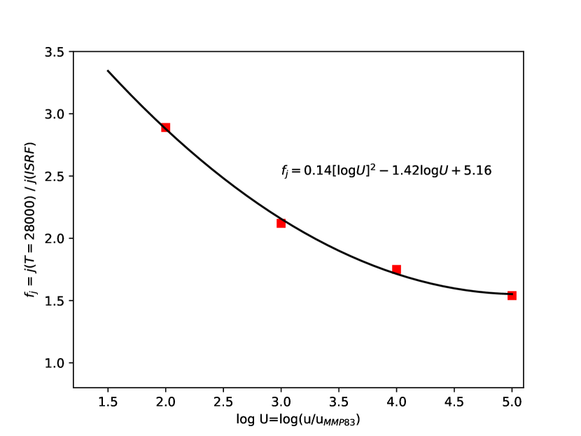
Figure 1: Ratio of Cloudy-derived dust emissivities, $f_{j}$, illuminated by a hot $T$=28,000 K source to illuminated by an interstellar radiation field having the same radiation density versus radiation density parameter, $U$.

Kobulnicky et al. (2018) used the dust emission coefficients of Draine & Li (2007, DL07) which are appropriate for an incident radiation spectrum similar to the mean interstellar one (Mathis et al., 1983), peaking in the red or near-IR portion of the spectrum. However, the spectrum from OB stars illuminating bowshock nebulae is much harder, peaking in the ultraviolet. Henney & Arthur (2019) concluded, on the basis of modeling an assortment of grain compositions using Cloudy (Ferland et al., 2017), that it was necessary to scale the DL07 emission coefficients upward by about a factor of three across a range of $10^{2}<U<10^{5}$ in order to replicate the emission coefficients at the same value of $U$. Henney & Arthur (2019, Figure 4) state that this is equivalent to using a DL07 model with a factor of about eight larger $U$. In the absence of tabulated data, we performed Cloudy modeling to compare the emissivity of standard ISM dust grains at 70 $\mu$m illuminated by a hot, $T$=28,000 K, $\log$ g=4.0 star (Castelli, & Kurucz, 2003) typical of our sample to emissivities illuminated by an interstellar radiation field (table ism in Cloudy) with the same radiation density. We define this ratio of emissivities, $f_{j}\equiv j(T=28000)/j(ISRF)$. Figure 1 plots $f_{j}$ versus radiation density parameter over the range of our sample objects, $U$=10²–10⁵. The black curve shows a polynomial fit to this relationship, $f_{j}(U)$=0.14[$\log$ U]${}^{2}-$1.42[$\log$ U]$+$5.16. At the low end of the range this ratio exceeds three, while at the high radiation densities it asymptotically approaches 1.5. Varying the modeled stellar effective temperature from 18,000 K to 45,000 K, representing the full range in our sample, shows that this ratio varies by about 15% across this wide range in temperature. Hence, a case-by-case, source-specific modeling effort would be appropriate as part of a future effort. In this present analysis, we will adopt the $f_{j}(U)$ from Figure 1 as a scale factor to increase the emission coefficients relative to nominal DL07 values to better approximate those expected in the UV-intense environments of bowshock nebulae . The net effect will be to decrease the derived mass-loss rates by factors of 1.5–3, with a median of 2.0. The correction is more significant for objects with lower radiation densities. These larger emission coefficients lead to reduced mass-loss rates compared to those in Kobulnicky et al. (2018), and all values here supersede that work.

We further note that our factor of 1.5–3 corrections to the DL07 dust emission coefficients, as indicated by Figure 1, are about 1.6$\times$ smaller than those adopted by Henney & Arthur (2019, Figure 4), which rely solely on Cloudy modeling. In other words, a direct comparison of dust emissivities from DL07 and those derived from Cloudy models for the same radiation density parameter and the same nominal interstellar radiation field and dust composition show that the former are a factor of about 1.6 smaller than the latter. We are unable to identify a reason for this difference (A. Li, private communication). Hence, the absolute values of the dust emission coefficients should be regarded to entail a systematic uncertainty at the level of 60% until systematic differences between DL07 and the dust implementation in Cloudy can be resolved.

2.3 Distinguishing Bowshocks from Radiation Bow Waves

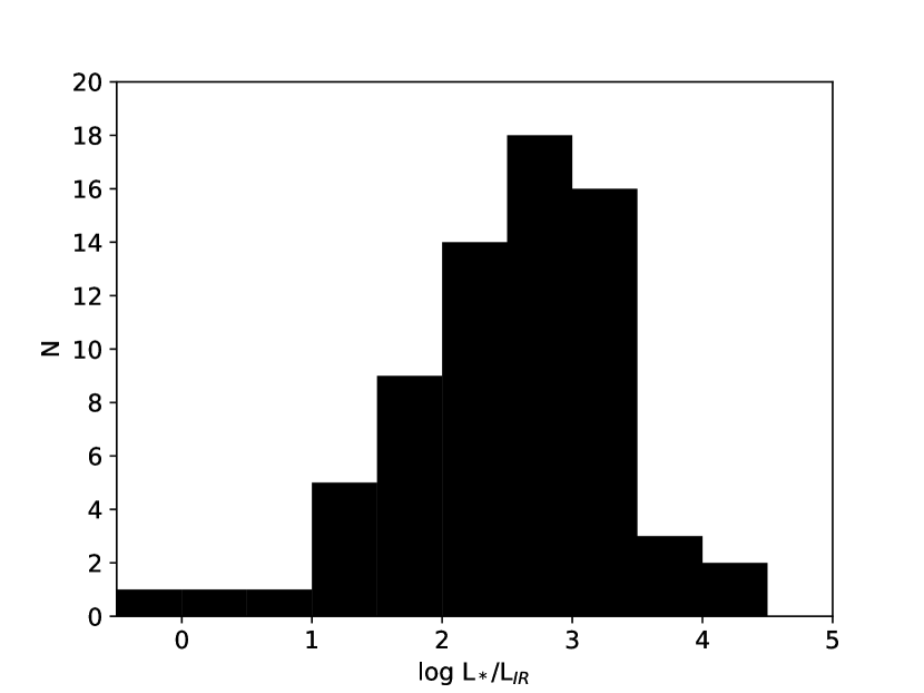
Figure 2: Histogram of the logarithm of the stellar luminosity to infrared nebular luminosity for the 70 objects in this sample. In objects with low values of $L_{*}/L_{\rm IR}$ the dust nebulae reprocess a significant fraction of the stellar luminosity, implying an appreciable optical depth for UV photons. The three lowest values are the three late-type stars in our sample.

Henney & Arthur (2019) articulated the physical distinction between stellar-wind-driven bowshocks and a class of “radiation bow waves” and “radiation bow shocks” that may appear morphologically similar but originate from radiation rather than stellar wind pressure as the dust and gas in a nebula becomes optically thick. Their Figure 2 distinguishes between these regimes as a function of three parameters: the stellar peculiar velocity, the standoff distance, and ambient interstellar density. It appears that our hottest and highest-velocity stars typically fall into the regime of true wind bowshocks, but a few objects, particularly the cooler ones, fall into the “radiation bow wave” regime. In the latter case, our derived mass-loss rates would become upper limits, as both stellar wind and radiation pressure play a role. We make a crude assessment of the physical status of each bowshock using the ratio of stellar luminosity to infrared nebular luminosity, $L_{*}/L_{\rm IR}$. This ratio ought to be large (e.g., $>$50) for true bowshocks where the dust optical depth is low and the nebula reprocesses a very small fraction of the stellar luminosity. Henney & Arthur (2019) analyzed the 20 bowshock stars presented in Kobulnicky et al. (2018) and concluded that all but two were likely to be true bowshocks. In particular, object #342 in the numeration of Kobulnicky et al. (2016) with $L_{*}/L_{\rm IR}$=22 is identified as an example of a trapped ionization front driving a radiation bow wave (Henney & Arthur, 2019). Figure 2 presents a histogram of $L_{*}/L_{\rm IR}$ for the sample. The three lowest bins show the three late-type stars in our sample which have $L_{*}/L_{\rm IR}<$10. We will tentatively regard the objects with $L_{*}/L_{\rm IR}<$75 (15 stars) as candidate bow-wave nebulae, based on the analysis that will follow in Section 4.1. The vast majority of the objects have $L_{*}/L_{\rm IR}>$75, making them likely to be genuine bowshock nebulae.

3 Sample Selection for Measuring $\dot{M}$

Beginning with the Kobulnicky et al. (2016) table of 709 infrared-selected bowshock candidate stars, we searched the GDR2 for corresponding parallax and proper motion measurements. We found that 486 of the 709 stellar targets had a corresponding entry in the GDR2 within 1.5 arcsec (a few sources had two $Gaia$ entries within that error circle, and the brightest was taken as the most probable source). However, we retained only the 231 stars for which the parallax:uncertainty ratio exceeds 3:1, indicative of a reliable distance. Of these 231, only 94 have bowshock nebulae with secure $HSO$ 70 $\mu$m detections required for estimating ambient densities (Kobulnicky et al., 2017). Distances computed straightforwardly from inverse parallaxes are known to be systematically too large owing to the resulting asymmetry from parallax error uncertainties (Bailer-Jones, 2015). Although our 3:1 parallax:uncertainty selection criterion minimizes this bias, we adopt the distances from the Bayesian treatment by Bailer-Jones et al. (2018), which results in 0% – 20% (mean of 7%) smaller distances compared to inverse parallax values. We also adopt as uncertainties their 68% confidence limits.

Figure 3 shows the locations on the Galactic plane of the 231 bowshock candidate stars with parallaxes known to 33% or better (filled circles). The Sun is at the center. Concentric circles illustrate 2 kpc and 4 kpc distances. Larger unfilled red circles denote the subset of 94 stars having detectable $HSO$ 70 $\mu$m nebulae. Clusterings within Figure 3 reveal the concentrations of bowshock OB stars in well-known Galactic associations such as the Cygnus-X region ($\ell\simeq 79^{\circ}$; $D$=1.4–1.8 kpc) and the Carina complex ($\ell\simeq 287^{\circ}$; $D$=2–3.5 kpc). The paucity of points in the second and third Galactic quadrants reflects the incomplete $SST$ 24 $\mu$m survey data in these regions, not necessarily a lower areal density of bowshock candidate objects. The relative lack of sources beyond 4 kpc reflects the reduced sensitivity and angular resolution of $SST$ surveys for distant targets in the bright, highly structured and confused mid-infrared images near Galactic mid-plane. Many of the bowshock candidates tabulated in Kobulnicky et al. (2016) are small, near the angular resolution limit of the telescope; more distant sources would appear point-like rather than arc-like and be excluded from the morphologically selected sample. Notably, nearly all of the objects in the fourth quadrant have 70 $\mu$m detections, while only about half in the first quadrant do. Finally, Figure 3 does not display obvious signs of spiral structure that might be traced by the OB stars as representative of young stellar populations. However, the portion of the Galactic plane covered is small, and features more distanct than 4 kpc would not be seen using this tracer. As noted by Xu et al. (2018), distance uncertainties on OB stars in GDR2 make discernment of spiral structure problematic even for samples much larger than ours. Furthermore, under the (yet-unvalidated and increasingly doubtful) hypothesis that bowshock stars are preferentially runaway stars, they may also fail to trace spiral structure if they have moved significantly from their birthplaces.

Our intended $\dot{M}$ analysis also requires a measurement of the stellar effective temperature for the calculation of the dust emission coefficient, $j_{\nu}$. This entails a secure spectral type for each target of interest. Of the 94 star/nebula pairs having parallax & proper motion data and 70 $\mu$m detections, we have collected spectral types for 70 stars. Our own optical and infrared spectra (as described above and in the Appendix) provide the majority of these; a minority come from the literature. A few of the tabulated targets are known or possible binary systems, noted as such in the Appendix. Because multiplicity is high among massive stars (Kobulnicky & Fryer, 2007; Sana et al., 2012), there are certain to be other undetected binaries among our sample. Most of the new observations obtained for this work entail only a single epoch of spectroscopy, making binaries difficult to identify. Nevertheless, the near-absence of double-lined spectra in our sample suggests that, even in systems containing two or more stars, one star dominates the luminosity. Notably, all but three of the 70 sample stars show He features, confirming that they are, overwhelmingly, OB stars. The remaining three non-OB stars turn out to be two (approximately) M giants (#129 and #289 in the numeration of Kobulnicky et al. (2016)) and one K giant (#653). Whether these three late-type stars are responsible for the nearby arcuate nebulae or whether they are unrelated field stars mistakenly identified is unclear. Ultimately, these are inconsequential, in a statistical sense, to the analysis that follows and are not discussed further.

Table 1 lists basic data for the selected subsample of 70 stars. Column 1 contains the index number using the numeration of Kobulnicky et al. (2016). Column 2 lists another common name of the star, followed by the generic name in Galactic coordinates in column 3. Column 4 provides the adopted spectral type/luminosity class, primarily from this work and references cited herein (see Appendix). Stars with an especially uncertain spectral type are designated by a colon. Columns 5 and 6 contain the adopted effective temperatures and radii, using the theoretical O-star temperature scale and radii from Martins et al. (2005a). For the few B stars we use the temperatures and radii of Pecaut & Mamajek (2013). Column 7 gives the adopted stellar mass, again from Martins et al. (2005a). Column 8 provides the adopted terminal wind speed calculated by averaging Galactic O and B stars of the same spectral type from Table A.1 of Mokiem et al. (2007) and Table 3 of Marcolino et al. (2009). An alternative approach to estimating terminal wind speeds based on the empirical calibration of (Kudritzki & Puls, 2000, equation 9) yields velocities 1.5 times larger, on average. The net effect of using these values would reduce derived mass-loss rates by the same factor, on average. Given the different effective temperature scales that undergird that relation, we elect not to adopt these larger terminal wind speeds. The adopted wind speeds are uncertain at the level of 30%, based on the dispersion at a given spectral type, and the fact that we do not have individual terminal wind speed measurements for these stars, which would obviously be desirable. Early B giants and supergiants are particularly uncertain with regard to both their wind speeds and stellar radii. Column 9 lists the parallax-derived distances from Bailer-Jones et al. (2018). The distances used here are generally consistent with those pre-$Gaia$ distances used in Kobulnicky et al. (2018), computed from other methods. The largest differences concern the six objects assumed to be part of the Cygnus OB2 Association at the 1.32 kpc eclipsing binary distance (Kiminki et al., 2015) but turn out to be much more distant, 1.7–1.9 kpc, according to $Gaia$ parallaxes. Column 10 lists the standoff distance, $R_{0}$, in arcsec, while column 11 lists the standoff distance in pc, calculated from the distance in column 9 and the angular separation and the statistical projection factor of 1.1. Column 12 lists the peak $HSO$ 70 $\mu$m surface brightness above adjacent background levels in 10⁷ Jy sr^-1, occurring at a location near the apex of the nebula. Column 13 lists the angular diameter in arcsec of the nebulae along a chord ($\ell$) intersecting the peak surface brightness, as described in the text and Figure 1 of Kobulnicky et al. (2018). Column 14 lists the source of spectral classification: “O” for optical spectroscopy from $APO$, “I” for infrared spectroscopy from $APO$, “C” for optical spectra from Chick et al. (2019), and “L” for literature spectral classifications. Column 15 lists the ratio of stellar to infrared nebular luminosity, $L_{*}/L_{\rm IR}$, calculated from the stellar parameters, distance, and infrared measurements from Kobulnicky et al. (2017).

Figure 4 is a histogram of the ratio parallax:uncertainty for the 394 candidate bowshock stars with entries in the GDR2 (gray shaded histogram). Some GDR2 entries list negative parallaxes and are not shown. Figure 4 illustrates that the majority of bowshock candidate stars have parallax data that are (at present) insufficiently precise for reliable distance and proper motion calculation. The black shaded histogram shows the 70 stars having known spectral types, 70 $\mu$m detections, and at least a 3:1 parallax:uncertainty ratio. Thus, the typical star retained for analysis has a distance known to 15% or better, which will reduce the uncertainties on $\dot{M}$ compared to those presented in Kobulnicky et al. (2018).

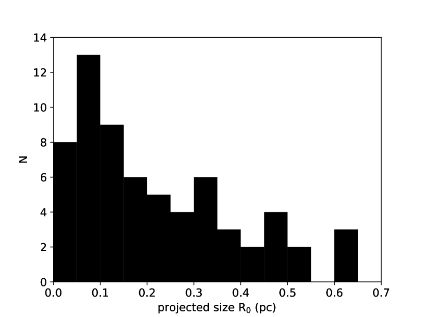
Figure 5: Histogram of the projected standoff distances, $R_{0}$ in pc for the 70 objects with well-determined distances and secure 70 $\mu$m nebular detections. The lowest bin is highly incomplete owing to the angular resolution limit of the $SST$ and $WISE$ observatories.

Figure 5 presents a histogram of the projected standoff distances, $R_{0}$, in pc, for objects with well-determined distances and secure 70 $\mu$m detections. The largest bowshock nebulae have characteristic sizes up to 0.6 pc, while 0.1–0.3 pc is typical. The smallest bins are incomplete because of the angular resolution limit of the $SST$ images. We expect that a 24 $\mu$m survey with arcsecond or better angular resolution would detect many additional arcuate nebulae, including objects at greater distances and objects with smaller standoff distances.

After distances, peculiar velocity, defined as the deviation from the star’s own local standard of rest, is the next most critical parameter. Proper motion, radial velocity, and distance, used in conjunction with a model for Galactic rotation, are sufficient to calculate the velocity of the star relative to its own local standard of rest. Ideally, precise radial velocity measurements would be available for each star. Unfortunately, the radial velocity uncertainties on most of the objects are appreciable, a consequence of calibration and random errors totalling 6–12 km s^-1. An even larger source of uncertainty is binarity. At least 50% of massive stars are found in binary systems where orbital velocities frequently exceed 100 km s^-1 (Kobulnicky et al., 2014). In order to prevent these sources of noise from dominating our estimate of peculiar velocities, we make the simplifying assumption that the stars’ velocity vectors are primarily in the plane of the sky. This is justified on the basis of the distinctive bowshock morphologies which would not be evident otherwise. Accordingly, we set the radial velocity component of each star to zero in its local standard of rest and compute the peculiar velocities solely from the two orthogonal components inferred from GDR2 proper motions. The reported peculiar velocities are, then, lower limits, but within 22% (i.e., $\sqrt{3}/\sqrt{2}$) of those expected in the case of isotropic three-dimensional velocities.

When computing peculiar velocities we apply the matrix transformation equations of Johnson & Soderblom (1987, also see Appendix A of () for implementation). These transformations were applied assuming Galactic Center coordinates $\alpha_{GC}$ = 17h:45m:37s.224, $\delta_{GC}$ =$-$28d:56m:10s.23 and Galactic North Pole coordinates $\alpha_{GNP}$ =12h:51m:26s.282, $\delta_{GNP}$ =27d:07m:42s.01 (Reid & Brunthaler, 2004). We adopt a solar galactocentric distance of 8.4 kpc and the Solar peculiar motion relative to the local standard of rest of (U,V,W)_⊙ = (11.1,12.2,7.2) km s^-1 (Schönrich et al., 2010). We adopt the Milky Way rotation curve of Irrgang et al. (2013, Model I). Our code for calculating peculiar velocities for bowshock stars uses the position, parallax, and proper motion for each star, removes the peculiar solar motion (U,V,W)_⊙, computes the expected (U,V,W)_∗ for the star’s Galactic position given the adopted rotation curve, and computes the peculiar (U,V,W)_∗pec velocity of the star, i.e., the star’s velocity relative to its local standard of rest. Our code reproduces the velocities of over 1000 K–M dwarf stars (Sperauskas, et al., 2016) to within 1.1 km s^-1 RMS. Uncertainties are propagated by Monte Carlo techniques. Table 2 lists the identification number (column 1), generic name in Galactic coordinates (column 2), GDR2 identifier (column 3), observed Heliocentric radial velocity (column 4), parallax and uncertainty in microarcseconds (columns 5 and 6), observed proper motions and uncertainties in right ascension in $\mu$as yr^-1 (columns 7 and 8) and declination in $\mu$as yr^-1 (columns 9 and 10). The radial velocities, which are certain to contain large contributions from unidentified binary orbital motion in some cases, are provided here for general interest only, and are not used further in this paper. The calculated space velocities, assuming zero radial velocity components, are reported in Table 3. In eleven cases the calculated space velocity is very small—less than five km s^-1. Given the documented bowshock morphology, the relative star-ISM velocity cannot be arbitrarily small. Such sources may be examples of “in-situ” bowshocks (Povich et al., 2008; Kobulnicky et al., 2016) caused by a bulk flow of ISM material. We arbitrarily impose a minimum velocity of five km s^-1 for these eleven objects.

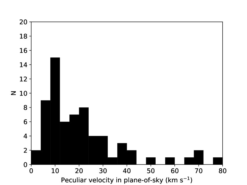
Figure 6: Histogram of stellar peculiar velocities relative to their local rest frame. The histogram depicts the 70  stars selected for analysis.

Figure 6 is a histogram of the stellar peculiar velocities, V_tot. Velocities range from near zero to 78 km s^-1. The mean and median peculiar velocities for the 70 sample objects is 15 and 11 km s^-1, respectively. There are no extreme-velocity stars in the sample, which is not surprising since such star are not expected to produce visible bowshocks (Meyer et al., 2016) The mean peculiar velocity of 30 km s^-1 assumed by Kobulnicky et al. (2018), is, in retrospect, overly large. However, there is a large dispersion of 16 km s^-1, so knowledge of each star’s individual peculiar velocity is important in the computation of mass-loss rates, given the $V_{\rm a}^{2}$ dependence. Figure 6 also reveals that the majority of bowshock-generating stars have a peculiar velocity less than 30 km s^-1 and would not, on this criterion, qualify as “runaway” stars. The possibility remains that some stars reside in regions of bulk ISM flows that introduce larger star-ISM relative velocities. Kobulnicky et al. (2016) noted that an appreciable fraction of bowshocks appear oriented toward a neighboring H II region where pressure gradients instigate ionized outflows and ISM velocities exceeding 30 km s^-1 are plausible (Tenorio-Tagle, 1979; Bodenheimer et al., 1979). Figure 5 of Kobulnicky et al. (2016) shows four bowshocks oriented toward the ionizing sources in the M 16 nebula. This is a good example of where bulk ISM flows may produce “in-situ” bowshocks (Povich et al., 2008) that do not require high-velocity stars.

Figure 7 is a histogram of the ratio peculiar velocity:uncertainty, where the uncertainties are obtained by Monte Carlo error propagation. The majority of stars have ratios less than 10:1. The median value for the 70-star subsample is 4.5, meaning that the typical velocity uncertainty is about 22%. Even with the new $Gaia$ data, velocity uncertainties remain significant when it comes to computing mass-loss rates, given the $V_{\rm a}^{2}$ dependence.

3.1 Computation of mass-loss rates

Table 3 contains quantities calculated from the basic data in Tables 1 and 2. Columns 1–4 contain the identifying numeral, name, generic name, and spectral type, as in Table 1. Column 5 contains the stellar luminosity in units of 10⁴ solar luminosities computed straightforwardly from the assigned effective temperature and radius. Column 6 contains the radiation density parameter, $U$, calculated from the basic stellar effective temperature, radius, and standoff distance. Column 7 lists the corresponding scaled 70 $\mu$m dust emission coefficient interpolated Column 9 is the ambient interstellar number density, $n_{\rm a}$, derived from the 70 $\mu$m specific intensity, the bowshock cord length, $\ell$ and the adopted $j_{\nu}$, as described by Kobulnicky et al. (2018, Equation 5). Densities range between 4 cm^-3 and 2100 cm^-3, with a median value of 20 cm^-3. These are typical of densities within the cool neutral phase ($\approx$30 cm^-3) and the diffuse molecular phase ($\approx$100 cm^-3) of the interstellar medium and much larger than the warm neutral phase ($\approx$0.6 cm^-3) (c.f., Draine, 2011, Table 1.3). Column 10 lists the peculiar velocity, V_tot, of the star derived from the proper motions, neglecting the radial velocity component. Column 11 gives its uncertainty. We caution that this velocity is only the best attempt at measuring the velocity of the star relative to its local interstellar medium. This velocity does not account for the possibility of local bulk flows of interstellar material, such as “Champagne flows” from a expanding H II regions. Columns 12 and 13 contain the mass-loss rates and corresponding uncertainties calculated from Equation 2. Values range from 6$\times$10^-10 $M_{\odot}$ yr^-1 to 5$\times$10^-5 $M_{\odot}$ yr^-1. Column 14 lists the difference between the logarithm of our derived mass loss rate and the logarithm of the theoretical mass-loss rate, calculated using Equations 24 and 25 of Vink et al. (2001).

In Kobulnicky et al. (2018) we assessed the uncertainties on $\dot{M}$ in terms of the uncertainties on each measurable parameter in Equation 2. The angular quantities $R_{\rm 0}$ and $\ell$ are measured to about 10% from infrared images, unchanged from our earlier work. $I_{\nu}$ is measured to about 20%, probably worse for some of the faintest nebulae. Mean stellar wind velocities are also unchanged, accurate to 30% and showing real variation from star-to-star (e.g., Mokiem et al., 2007). Similarly, the uncertainty on $j_{\nu}$ is driven by the uncertainties on stellar temperature (taken to be 2000 K), radius (10%), and standoff distance (we use the actual tabulated uncertainties), however systematic uncertainties on the absolute values may exist at the 60% level. Stellar distances and velocities—previously the dominant sources of uncertainty — are now known much more precisely by virtue of the new $Gaia$ data, but still have significant uncertainties as shown in Figures 4 and 6 and by the data in Table 3. We calculate uncertainties on the mass-loss rates using a 1000-iteration Monte Carlo error propogation procedure with the aforementioned uncertainties as inputs. Our procedure would ideally start with the basic $Gaia$ parallax and proper motion measurements for a proper ab inito error analysis. However, since we lack access to the Bailer-Jones et al. (2018) Bayesian code, we adopt the nominal distances and uncertainties from that work as well as the nominal stellar peculiar velocities and uncertainties they imply in order to further propagate the uncertainties from stellar temperature, radius, wind speed, and nebula angular quantities from Equation 2. We find that a significant fraction of the iterations would result in unphysical negative peculiar velocities if the nominal velocity errors were used, e.g., 2$\pm$1 yields a non-negligible fraction of negative values. This, combined with the likelihood that bulk ISM flows are an appreciable component of the star-ISM relative velocity, leads us to exclude velocity uncertainties from the Monte Carlo error analysis. Therefore, the ensuing uncertainties on $\dot{M}$ appearing in the last column of Table 3, should be regarded as indicative lower bounds. The average uncertainty is 42% (excluding uncertainties on dust emission coefficients and stellar peculiar velocities).

4 Analysis

4.1 Presentation of Mass-Loss Rates

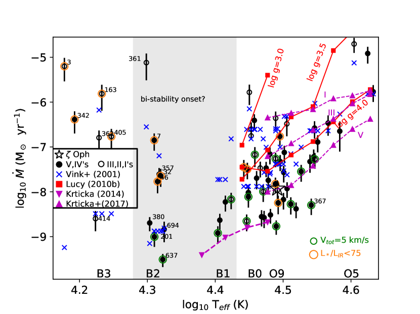
Figure 8: Mass-loss rate versus stellar effective temperature. Black filled points and black open circles depict measurements for main-sequence and evolved stars from this sample, respectively. Blue crosses mark predictions for each object using the expressions of Vink et al. (2001, Equations 24 & 25). Red squares and lines show the model predictions of Lucy (2010b) for nominal main-sequence ($\log$ g=4.0), giant ($\log$ g=3.5), and supergiant ($\log$ g=3.0) stars, as labeled. The triangles and dotted lines show the theoretical predictions of Krtička (2014) and Krtička & Kubát (2017) for B and O stars, respectively. Green circles identify stars where the stellar peculiar velocity, $V_{\rm tot}$, has been arbitrarily fixed to the minimum values of 5 km s^-1. Orange circles enclose objects that are candidate radiation bow wave nebulae. Two evolved B stars from Table 3 lie off the left side of this plot, as do the three cool late-type stars. A gray band marks the expected region of the bi-stability phenomenon.

Figure 8 plots the calculated mass-loss rates versus stellar effective temperature. Black filled symbols denote the sample objects: a star for $\zeta$ Oph, filled circles for luminosity class V and IV stars, and open circles for giants and supergiants. A small dispersion has been added to the data points along the temperature axis to prevent marker pile-up. Green circles enclose the objects where the peculiar velocities were set to the minimum value of 5 km s^-1. Not surprisingly, these lie near the lower edge of the distribution. Orange circles mark the objects having $L_{*}/L_{\rm IR}<$75 as potential radiation bow waves. This criterion was selected based on the principles outlined in Henney & Arthur (2019) and after some experimentation that showed this cutoff selects all of the low-temperature stars with excessively large implied mass-loss rates but only a few of the hotter stars. Two mid–late B stars from Table 3 lie off the left side of this plot, as do the three cool late-type (K–M) stars. Blue crosses depict model predictions for each object using the formulation of Vink et al. (2001, Equations 24 and 25) computed using the stellar data from Table 1. We assume $v_{\infty}/v_{\rm esc}$=2 for stars on the hot side of the bi-stability jump and 1.3 for the cool side, per Vink et al. (2001). Hence, each filled data point is paired vertically with a blue $\times$ at the same temperature, although the $\times$’s sometimes overlap. Red squares connected by lines depict the model predictions from Lucy (2010b) for (approximate) main-sequence ($\log$ $g$=4.0) and giant ($\log$ $g$=3.5) and supergiant ($\log$ $g$=3.0) stars, as labeled. Magenta triangles and dashed lines show the predictions for B main-sequence stars from Krtička (2014, solar abundance models) and O stars (Krtička & Kubát, 2017), with separate tracks for stellar luminosity classes I, III, and V. A gray band marks the predicted regime of the bi-stability jump.

For the hot portion of the sample, the data show mass-loss rates rising from few$\times$10^-9 $M_{\odot}$ yr^-1 near 27,000 K to over 10^-6 $M_{\odot}$ yr^-1 for O5 stars near 42,000 K, but with a large dispersion of about half an order of magnitude. The data points for stars B1 and earlier fall systematically below the Lucy (2010b) and Vink et al. (2001) predictions, but broadly consistent with—if slightly above—the Krtička (2014) and Krtička & Kubát (2017) models. The results are similar to those of Kobulnicky et al. (2018) but for a sample more than three times as large extending to cooler temperatures. The dispersion of the data is larger than the typical uncertainties in the vertical dimension, consistent with additional uncertainty terms and/or real variations. Considering the $\pm$1 subtype uncertainty on classifying any particular star, especially early B stars, any given object may fall into an adjacent temperature bin. Evolved stars (open circles) generally lie above the luminosity class V and IV stars, also in accord with model predictions.

The prototypical bowshock star $\zeta$ Oph, in particular, shows good agreement with the Krtička & Kubát (2017) models. With $L_{*}/L_{\rm IR}=$1700, $\zeta$ Oph is safely out of the dust bow wave regime and should represent a good point of reference to studies employing other techniques. Our nominal derived $\dot{M}$ of 1.2$\times$10^-8 $M_{\odot}$ yr^-1 is a factor of 15 lower than the estimate of 1.8$\times$10^-7 $M_{\odot}$ yr^-1 from Repolust et al. (2004), which assumed no wind clumping correction, and hence, must be regarded as an upper limit. Had we included the radial velocity component of $\zeta$ Oph’s total space velocity (as one of the stars where the assumption of zero radial velocity is known to be inconsistent with the data), the resulting space velocity of 26 km s^-1 would imply a mass-loss rate of 5.5$\times$10^-8 $M_{\odot}$ yr^-1, still considerably lower than Repolust et al. (2004), but only by a factor of three, which would be consistent with a standard correction for wind clumping. Differences in adopted stellar parameters ($v_{\infty}$=1550, R_∗=8.9 R_⊙, T_eff=32,000 K versus 1300/7.2/31,000 adopted here) are relatively minor effects. Repolust et al. (2004) notes that this star is a rapid rotator with $V_{\rm r}$$\sin$ $i$=400 km s^-1 which could induce non-isotropic winds and modify the published values in either the observational or theoretical analyses, or both. Our derived mass-loss rate for $\zeta$ Oph is still a factor of 10 or more larger than the $\dot{M}$=1.5$\times 10^{-9}$ $M_{\odot}$ yr^-1 inferred from an analysis of X-ray line profiles (Cohen et al., 2014) or the 1.6 $\times$10^-9 $M_{\odot}$ yr^-1 from UV absorption lines (Marcolino et al., 2009). Hence, there remains a considerable discrepancy between observational results on this prototypical “weak wind” late-O star.

B1 and later spectral types in Figure 8 fall considerably above the Krtička (2014) prediction and above an extrapolation of the Lucy (2010b) models. These stars lie within the predicted regime of the bi-stability discontinuity. They show a large dispersion in mass-loss rates from $<$10^-9 $M_{\odot}$ yr^-1 to almost 5$\times 10^{-5}$ $M_{\odot}$ yr^-1, approaching — but not exceeding — the very large mass-loss rates predicted by Vink (2018) for LBV stars, in a few instances. Notably, a majority of the stars in this regime are candidates for being dust bow wave objects, having $L_{*}/L_{\rm IR}<$75, making their derived mass-loss rates suspect. However, the positions of some of these stars, particularly those that are not bow wave candidates, are broadly consistent with the Vink et al. (2001) prescriptions that take into account the effects of bi-stability below $\simeq$27,000 K.

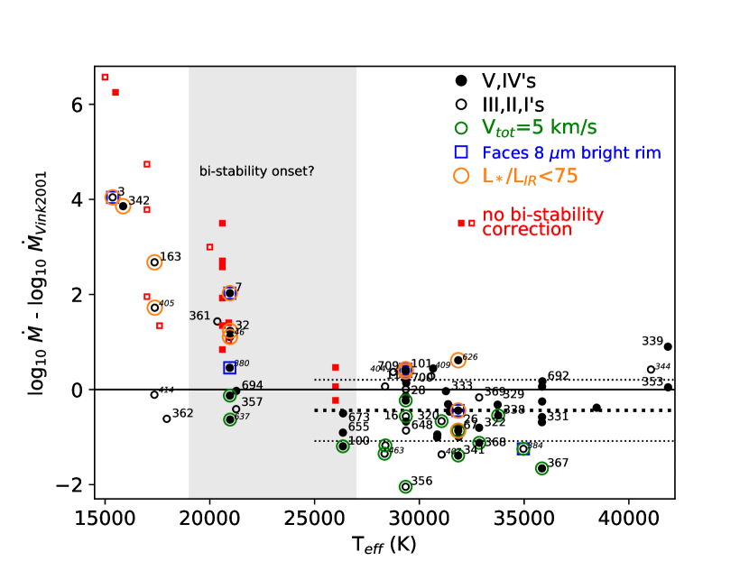
Figure 9: The log of the mass-loss rate derived in this work minus the log of the Vink et al. (2001) prescription versus effective temperature. Numerical labels identify stars having H$\alpha$ spectra presented in Figure 10 (larger font) and other objects of interest (smaller italic font). Black symbols denote comparisons performed using the Vink et al. (2001) upper/lower branch formulae for objects above/below 27,000 K, respectively. Red symbols show stars having $T_{\rm eff}<$27,000 K if the upper branch prescription neglecting bi-stability effects were used instead. Green circles mark objects where the lower limit peculiar velocity of 5 km s^-1 was assigned. Orange circles enclose objects that are candidate radiation bow wave nebulae. Blue squares enclose objects that directly face an 8 $\mu$m bright-rimed cloud.

Figure 9 plots the difference of the logarithms between the mass-loss rates derived in this work and those predicted by the Vink et al. (2001) formulation versus effective temperature. As before, filled markers denote (near-) main-sequence objects and open circles denote giants and supergiants. A gray band highlights the range of the expected bi-stability jump. Numerals adjacent to symbols identify each object, with a larger font for objects having our own optical spectroscopy and smaller italic font for other stars. Black symbols denote comparisons performed using the Vink et al. (2001) upper/lower branch formulae for objects above/below 27,000 K, respectively. Red symbols show stars having $T_{\rm eff}<$27,000 K if the upper branch prescription neglecting bi-stability effects were used instead. Green circles enclose objects where the lower limit peculiar velocity of 5 km s^-1 was assigned. Orange circles enclose candidate bow wave objects having $L_{*}/L_{\rm IR}<$75. Blue squares enclose objects that directly face an 8 $\mu$m bright-rimed cloud where photoevaporative flows from the molecular cloud interface may influence the infrared nebulae. Horizontal dashed lines mark the mean (bold dotted) and dispersion (non-bold dotted) for all points above 25,000 K. The mean lies at $-$0.43 dex, indicating that, on average, the mass-loss rates are a factor of 2.7 below the Vink et al. (2001) prescription in in this regime, with a considerable dispersion of 0.64 dex (factor of 4). A direct comparison with the predictions of Krtička & Kubát (2017) is not possible owing to the limited number of models tabulated in that work, but it may be concluded from Figure 8 that our inferred mass-loss rates lie, on average, above those values by 0.1–0.3 dex. The large dispersion in the data points in this figure results partly from the uncertainties on the derived mass-loss rate, typically 0.2–0.3 dex (see Table 3, but recall that the tabulated uncertainties here do not include errors in $V_{\rm a}$), systematic errors on dust emission coefficients, or additional uncertainties on the computed theoretical Vink et al. (2001) mass-loss rate (driven by uncertainties on the adopted parameters including the stellar luminosity, mass, effective temperature, terminal wind speed, and metallicity), amounting to another $\sim$0.2–0.3 dex.

Figure 9 demonstrates that there is a systematic difference between our mass-loss estimates and theoretical models at temperatures $>$25,000 K and a much larger dispersion in mass-loss rates for stars $<$25,000 K. The agreement between data and models is better when the prescription for bi-stability is applied—that is, the positions of black data points are consistent with the models minus a small offset versus the red symbols which depart dramatically from the predictions toward lower temperatures). Unfortunately, our spectra do not contain the Si II and Si III lines in the blue portion of the optical spectrum required to assign temperatures to hot stars, so we are unable to ascertain the operative temperature where this deviation begins. Realistically, enhanced mass loss may become evident over a range of temperatures and luminosities depending on other factors traditionally linked to wind strength such as the stellar mass, metallicity, and rotation rate. Indeed, Crowther et al. (2006) identified a systematic drop in terminal wind speeds across a 4000 K range in a sample of B supergiants but, these authors, as well as Markova & Puls (2008) did not find a corresponding increase in mass-loss rates. Hence, our data in Figures 8 and 9 could represent the first evidence for enhanced mass-loss associated with the bi-stability phenomenon. In particular, the most reliable data points (those without orange circles) show reasonable agreement with the Vink et al. (2001) predictions, falling below the horizontal line by about 0.43 dex, similar to the hotter portion of the sample. An extrapolation of the heavy dotted line marking the mean of the $T_{\rm eff}>25,000$ stars would intersect the most reliable B2–B3 objects in our sample, provided that the proper bi-stability formulation is used to predict the theoretical values. Our estimate of the mass-loss rates for these objects, $\simeq 10^{-9}$ $M_{\odot}$ yr^-1, for the four B2V stars represents the first results for dwarf stars in this temperature regime. Their values are, like the hotter potion of the sample, about a factor of 2.5 below the Vink et al. (2001) predictions.

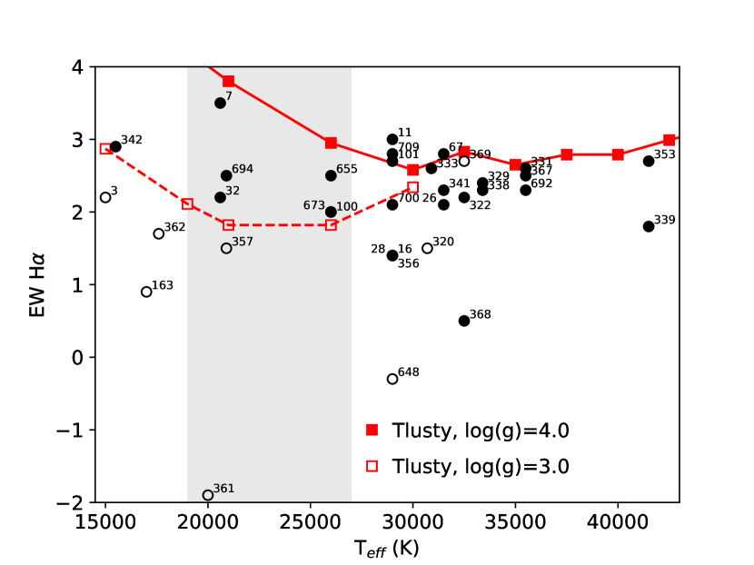
Figure 10: H$\alpha$ equivalent width versus effective temperature for 37 stars with suitable data. The red points and lines are the expectations for dwarf and supergiant gravities from theoretical model spectra with no mass loss (Lanz & Hubeny, 2003).

If the especially high rates of mass loss for some cool objects were taken at face value, it ought to imprint an observable signature in the spectra in the form of extraphotospheric H$\alpha$ emission. While we do not have high-resolution optical spectra of the sample stars that would be required to detect low levels of emission in the line cores, we do have low-resolution spectra for 37 stars. Figure 10 plots the observed H$\alpha$ equivalent width versus stellar effective temperature for the sample stars with suitable data. Solid circles represent main-sequence stars and open circles represent evolved stars, as in previous figures. Numerals designate each object by identification number. The red squares and lines mark theoretical values from model atmospheres (Tlusty, Lanz & Hubeny, 2003, the O and B-star grids for solar metallicity) which are appropriate to plane-parallel static atmospheres without a wind. Positive values represent absorption and negative values represent emission, per conventional usage. While the equivalent width of H$\alpha$ is expected to increase from hot to cool (simply because Balmer lines becomes stronger toward cooler stars in this temperature range) across the bi-stability region, the data are mostly flat or decreasing, consistent with seeing elevated mass loss over the 27,000–19,000 K regime. Most points in this range lie below theoretical expectations consistent with a small contribution from extraphotospheric emission. The lack of strong emission lines from the cool objects with very high implied mass-loss rates in Figure 8 suggests that the infrared nebulae in such objects are driven by radiation pressure not winds, consistent with their small $L_{*}/L_{\rm IR}$ ratios.

A comparison of outliers in Figures 8, 9, and 10 provides a means of assessing whether mass-loss rates are internally consistent. Considering first the coolest objects at the left edge of both figures, the B4V #342 and the B5III #3 have derived mass-loss rates four orders of magnitude above the model predictions, even when bi-stability effects are considered. Both objects have $H\alpha$ substantially in excess of the stellar photosphere, but not in emission, as might be expected for such large mass-loss rates. While both objects have nebular surface brightnesses among the highest in the sample, they are not extraordinary in this regard. But they are extraordinary in that the nebular surface brightesses are high for their late (cool!) spectral type. Both nebulae are bright at 8 $\mu$m, indicating PAH emission consistent with a molecular cloud interface. Furthermore, #3 faces an 8 $\mu$m bright cloud rim (Kobulnicky et al., 2016, Figure 13.3), and is among the objects considered by Kobulnicky et al. (2016) to be affected by a photoevaporative flow from the inner edge of that rim. The extent of the impacts from this phenomenon has not been theoretically developed. Both #3 and #342 have $L_{*}/L_{\rm IR}<75$, making them probable radiation bow waves. Among the four evolved $\simeq$B3 stars, #163 (B3II) and #405 (B3III) lie 2–3 orders of magnitudes above Vink et al. (2001) predictions while #362 (B2I) and #414 (B3II) lie close to the model predictions. H$\alpha$ for #163 lies well in excess of the model photosphere (but not in emission). This nebula lies along a 70 $\mu$m filament that does not show good morphological correspondence with the 24 $\mu$m nebulae. It is likely that this object is confused by unrelated foreground or background emission. In the case of #405, we do not have H$\alpha$ data. It faces the IC2599 H II region associated with the energetic young cluster NGC 3324, which may drive an outflow and create a relative star-ISM velocity in excess of the tabulated 7.7 km s^-1. Both #163 and #405 are probable radiation bow wave nebulae. Objects #362 and #414, on the other hand, agree well with model predictions once bi-stability behavior is considered. Neither object has evidence for being an instance of the radiation bow wave phenomenon.

Stars in the B2 temperature range show mass-loss rate estimates in better agreement with model predictions, on average, but some still lie far above expectations in Figure 9. Object #7 (B2V), for example, lies two orders of magnitude above Vink et al. (2001) predictions in Figure 9. Like, #3, it is a probable radiation bow wave nebula. It faces a bright-rimmed cloud prominent at 8 $\mu$m and may be affected by a photoevaporative flow (Kobulnicky et al., 2016, Figure 13.7). Examination of the mid-infrared image in Kobulnicky et al. (2016) shows another star 40″ to the southwest of the nebulae that also lies along the nebula axis of symmetry. Identified as an AGB star candidate (Robitaille et al., 2008), 2MASS J17582964-2610138 (R.A.(2000)=17h:58m:29s.64, Dec.(2000)=$-$26d:10m:13s.8) has H=10.4 mag and $A_{\rm K}$=3.08, an implied extinction that apparently precludes its inclusion in the GDR2, so its distance is unknown. If this star is the source of luminosity powering the nebula it should be marked with an open circle in Figures 8 among other luminous evolved cooler stars. This object should be regarded as uncertain in all respects. Object #361 (B1Ia; highly uncertain type and luminosity class) has a 70 $\mu$m nebula that is very near the detection limit, and the background is correspondingly very uncertain. The derived mass-loss rate could be considered an upper limit. Object #32 (a probable B2V+B2V binary) lies near an extended 70 $\mu$m nebulosity that makes the background level somewhat uncertain. It is also a radiation bow wave candidate. Object #46 (B2V; also a radiation bow wave candidate) has an unusually large implied reddening for its parallax distance ($D_{\rm par}$=688${}^{+163}_{-111}$ pc; $A_{\rm V}\simeq$11 mag; see Appendix), which may have implications for its nature and derived mass-loss rate. Object #380 (B2Ve) also lies faces a bright-rimmed cloud, a feature in common with other stars that show above-predicted mass-loss rates in Figure 9. The remaining four objects in this temperature regime (#694–B2V, #201–B2V, #357–B2III, and #637–B2V) all show mass-loss rates near the predicted values, and they all appear to be isolated objects with well-defined nebulae. These objects comprise what we believe to be the first collection of B2 dwarfs with measured mass-loss rates, although two of these have the assigned minimum peculiar velocity of 5 km s^-1.

The next group of three hotter stars near B1 shows improved agreement with the theoretical predictions. All three lie slightly above the Krtička (2014) prediction in Figure 8 but substantially below the Vink et al. (2001) prediction, best visualized in Figure 9. Our data represent the first estimate of mass-loss rates for dwarfs of this temperature class.

Other outliers in Figure 9 merit some discussion. Object #101 (B0V) faces an 8 $\mu$m bright-rimmed cloud and is a possible radiation bow wave with $L_{*}/L_{\rm IR}<75$ . Object #626 (O9V) is also a radiation bow wave candidate, having the second highest nebular surface brightness in our sample. Object #339 (O5V) has one of the largest nebulae in our sample, and it has the largest peculiar velocity (78 km s^-1). It also displays an H$\alpha$ EW considerably in excess of the photosphere in Figure 10. Object #344 (the well-studied O4If star BD+43 3654) has the highest mass-loss rate in our sample (5$\times$10^-5 $M_{\odot}$ yr^-1), somewhat in excess of predictions. There is the possibility that many of these objects are unrecognized binaries, and that their derived mass-loss rates should be reduced accordingly — 0.3 dex for equal-luminosity components. Objects that fall far below expectations are often those where the minimum peculiar velocity of 5 km s^-1 has been assigned. These include #356 (B0III), #463 (B0III), #341 (O9V), and #367 (O7V). One other evolved object, #407 (O9III+O), is a radiation bow wave candidate, but falls far below model expectations. Object #407 could also be an in-situ type bowshock as it does face directly toward the very energetic Carina star-forming complex at an angular separation of $\simeq$0$\fdg$2. As such, its peculiar velocity may underestimate its true star-ISM velocity. Conversely, object #409 (O9.5IV) lies above model predictions and also faces the Carina nebula.

4.2 An Investigation of Biases by Subsample

In an effort to investigate whether sample selection effects impact the essential conclusions from Figure 8, we considered only the half of the sample having nebular surface brightness above the median value. We found that the essential conclusions from Figure 8 are unchanged, with the O stars and early B stars showing good agreement with models and having a similar dispersion as in the full sample. However, fewer of the cooler stars are retained in this cut, indicating that the majority of the high-surface-brightness nebulae are, unsurprisingly, associated with hotter stars. The lower surface brightness of the nebulae associated with the B stars in this sample means that they carry larger uncertainties, by virtue of the difficulty defining and subtracting local background emission around each nebula. We also replicated Figure 8 for the half of the sample having the highest velocity precision (indicated by peculiar velocity:uncertainty ratio $V_{\rm tot}$/$\sigma_{V}$)above the median value of 4.5. The essential elements of Figure 8 remain. O stars and early B stars show good agreement with the models and have a similar dispersion as before while the cooler stars exhibit the same dispersion observed in the full sample. We conclude that including stars with larger velocity uncertainties does not bias the results in any particular direction. Figure 11 replicates the full set of objects from Figure 8, but magenta hexagons now enclose nebulae having 8 $\mu$m detections, suggestive of possible PAH contributions. Sources with 8 $\mu$m detections lie scattered throughout the Figure, occurring both a low and high temperatures as well as at low and high mass-loss rates. However, at the cooler end of the temperature range, most of the points that fall far above above the expected trend are those with PAH detections. Many among this subset are also radiation bow wave candidates. Hence, at high temperatures the presence or absence of PAH features does not appear to bias the data in any particular direction, but at low temperatures it may be wise to treat such objects with caution.

Table 4 provides a list of object ID numbers that fall into each of the aforementioned special categories. These are the 11 objects having $V_{\rm tot}<$ 5 km s^-1, the seven objects that face 8 $\mu$m bright-rimmed clouds, and the 15 candidate bow-wave objects having $L_{*}/L_{\rm IR}<75$.

4.3 The Wind-Luminosity Relation

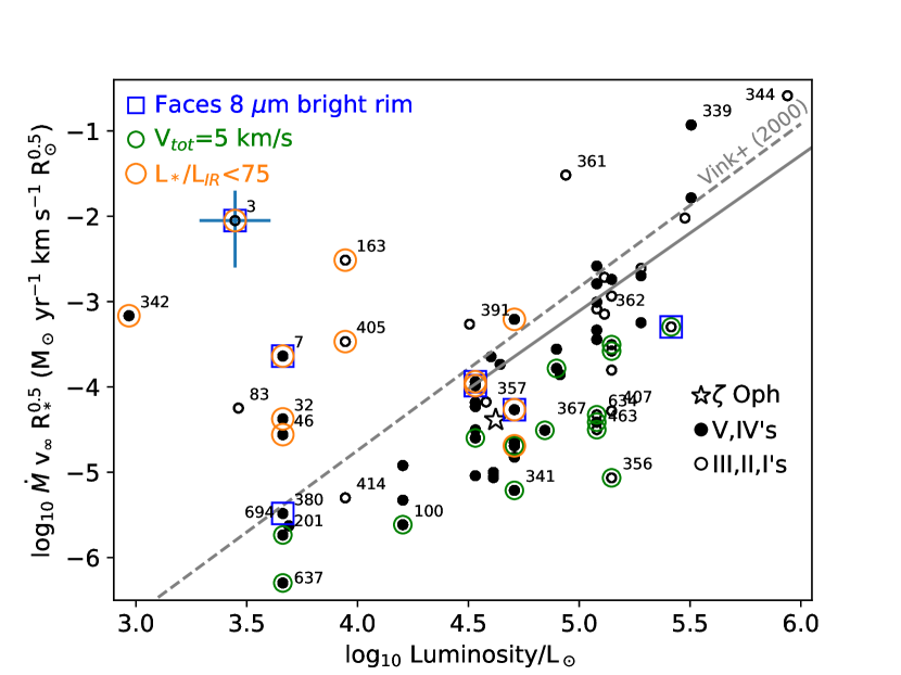
Figure 12: Modified wind momentum versus stellar luminosity. The gray solid and dashed lines denote the theoretical relations for stars 27,500–50,000 K and 12,500–22,500 K, respectively (Vink et al., 2000). Filled circles denote luminosity class V and IV objects while open circles are luminosity classes I–III. Because of the log scale, the uncertainties are similar for all data points; a single error bar denotes typical uncertainties.

Figure 12 plots the modified wind momentum (Kudritzki et al., 1995, the product of mass-loss rate times terminal wind speed times square root of the stellar radius) versus stellar luminosity. Filled circles denote luminosity class V and IV objects while open circles are luminosity classes I–III. As in Figure 8, blue squares enclose objects that face an 8 $\mu$m bright-rimmed cloud, while green circles enclose objects where the minimum peculiar velocity was assigned, and orange circles enclose objects that are candidate radiation bow waves, $L_{*}/L_{\rm IR}<75$. Because of the log scale, the uncertainties are similar for all data points. A single error bar denotes typical uncertainties which are dominated by the temperature uncertainty of 10% (x-axis) and the uncertainties on the mass-loss rates (Table 3) and terminal wind velocities (y-axis). The gray solid and dashed lines are theoretical relations for stars 27,500–50,000 K and 12,500–22,500 K, respectively (Vink et al., 2000, Equations 15 and 17), representing both sides of the nominal bi-stability jump.

The dispersion among the data points is large, but a correlation is clear, consistent in slope with the theoretical wind-luminosity relation. The data fall systematically below this theoretical relation by about 0.4 dex. Notably, the green circles fall exclusively on the low side of the trend and below model predictions. Most of the objects that lie above model predictions are candidate radiation bow waves, and these often coincide with nebulae that face an 8 $\mu$m bright-rimmed cloud. The most deviant objects in Figure 8, #3, #163, #342, and #361, also lie furthest from the theoretical relation in this figure. Possible reasons for their departure from theoretical expectations have been discussed earlier. The cool (B5–B8II, but highly uncertain) objects #83 and #391 appear on this plot but not on previous figures where they fall off the cool end of the axis range. Both lie considerably in excess of the predicted relation, but neither is identified as a probable radiation bow wave nebula. Both objects are cool enough that the second bi-stability jump near 10,000 K may be relevant. Object #361 (B2I) also lies well above the expected relation, but its temperature and luminosity is very poorly constrained by the available data. Once the candidate radiation bow wave nebulae are removed, the remaining data in Figure 12 show good agreement with the slope of the theoretical wind-luminosity relation, but with a zero point offset of about 0.4 dex toward lower values.

4.4 Comparison with Prior Data

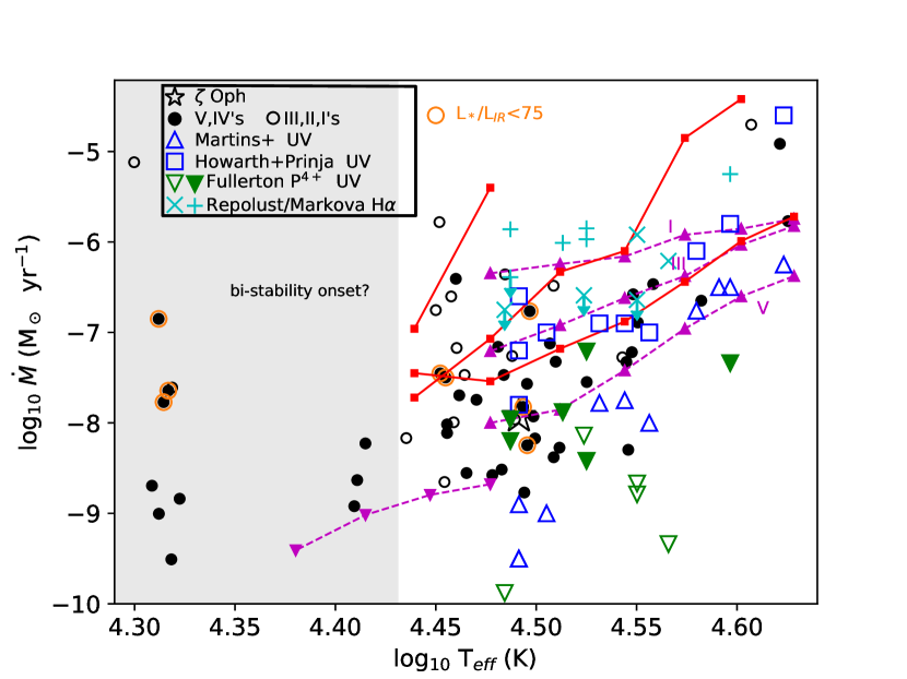
Figure 13: Mass-loss rate versus effective temperature for dwarfs (filled circles) and evolved stars (open circles) from the bowshock sample. Open blue triangles and squares depict observational results from the sample of Galactic O3–O9 main-sequence stars as measured by Martins et al. (2005b) and Howarth & Prinja (1989), respectively. Green open and filled triangles depict the dwarfs and giants, respectively, measured using the ultraviolet P⁴⁺ line (Fullerton et al., 2006). Cyan $\times$’s and $+$’s depict the same stars as determined from the H$\alpha$ line (Repolust et al., 2004; Markova et al., 2004). Red and magenta lines mark theoretical predictions, as in previous figures.

Figure 13 replicates Figure 8 and includes mass-loss rates measured for the set of Galactic O3–O9.5 dwarf stars from Martins et al. (2005b) (blue open triangles) and Howarth & Prinja (1989) (blue open squares), respectively. The Martins et al. (2005b) mass-loss rates derived from UV spectra fall somewhat below the bowshock sample, increasingly so in the regime of late O stars. The mass-loss rates given by Howarth & Prinja (1989) lie consistently above those in the present sample. The Howarth & Prinja (1989) values are broadly consistent with the Lucy (2010b) theoretical expectations for dwarfs, but above the Krtička & Kubát (2017) relation. Figure 13 also shows the late-O dwarf and giant stars with mass-loss rates determined from ultraviolet P⁴⁺ absorption lines (Fullerton et al., 2006, green open and filled triangles, respectively) and the same set of stars determined from the H$\alpha$ line (Repolust et al., 2004; Markova et al., 2004, cyan x’s and +’s). The P⁴⁺-based estimates show a large dispersion and lie consistently below the mean of the bowshock sample, but there is some overlap. The H$\alpha$ results (for homogeneous winds) lie far above the mean of the bowshock stars by factors of ten or more. Some are upper limits, indicated by arrows, and are consistent with the bowshock estimates. This suggests that corrections for clumping in stellar winds are significant, factors of 3–10, consistent with inferences from other works (e.g., review by Puls et al., 2008). Unfortunately there are no objects in common (with the exception of $\zeta$ Oph) between the bowshock sample and the UV-based and H$\alpha$-based studies, so direct comparisons must await future works. Overall, Figure 13 shows the bowshock sample agrees reasonably well with UV-based estimates, but lacks examples of extremely low mass-loss rates $\dot{M}<10^{-9}$ $M_{\odot}$ yr^-1 that typify the weak-wind phenomenon. The bowshock sample also extends observational results into the regime of B0–B2 dwarfs that are not probed by other methods.

5 Discussion and Conclusions

Application of the physical requirement for momentum balance between a stellar wind and an impinging ISM yields a new method of mass-loss measurements for a sample of 67 early type stars. The inferred relation between mass-loss rate and stellar temperature & luminosity agrees well with several sets of theoretical models for main-sequence and evolved stars hotter than about 25,000 K, especially when models accounting for bi-stability behavior are employed, e.g., Figure 9. However, the mean mass-loss rates are lower by factors of about 2.7 compared to the canonical Vink et al. (2001) prescription, even allowing for a reduction of theoretical rates required by adoption of lower solar metallicity. This factor of $\simeq$2.7 is consistent with the proposed reductions of 2–3 discussed in the literature and inferred from other measurement methods (summarized by Puls et al., 2015). The derived mass-loss rates are in reasonable agreement with–but slightly larger than–the theoretical predictions of Krtička & Kubát (2017). Our data represent the first mass-loss estimates for dwarf stars in the very late-O and early B spectral ranges.

At temperatures cooler than 25,000 K the agreement is less good but is considerably better when bi-stability physics is applied rather than neglected, i.e., the black versus the red points in Figure 9. We interpret this better agreement as a soft empirical confirmation that the prescriptions of Vink et al. (2001) get the temperature range and magnitude of bi-stability effects approximately correct. Some of the cool objects in Figure 9 show excellent agreement with predictions while others show exceedingly high mass-loss rates compared to models. Some of these large deviations may be explained by additional effects, such as when stars facing an 8 $\mu$m bright-rimmed cloud experience an impinging photoevaporative flow which amplify the nebular surface brightness. Five of the seven such objects in our sample (blue squares in Figures 9, and 12) show elevated mass-loss rates compared to predictions. The majority of the most discrepant data are also probable radiation-driven bow waves where the nebula is becoming optically thick to UV photons. In these cases, the inferred mass-loss rates can be regarded as upper limits. Such objects should be discarded from efforts to measure mass-loss rates unless corrections can be developed. In the few cases where the derived mass-loss rates lie below predictions, some of these objects face giant H II regions where bulk outflows may produce a greater star-ISM relative velocity than we derive from $Gaia$ proper motions, leading to an underestimate of $\dot{M}$. For some objects $Gaia$ proper motions imply an unrealistically low peculiar stellar velocity, given the distinct arcuate nebulae observed, so we have assigned a minimum $V_{\rm tot}$ of five km s^-1. Ten of the eleven such stars show mass-loss rates below the mean of the sample, leading us to consider these estimates of the mass-loss rates to be lower limits. This sample, as a whole, exhibits the power-law relation between modified wind momentum and luminosity very similar in slope—but not in zero point—to that predicted from classical wind momentum arguments (Figure 12). Outliers on this Figure closely track the deviations observed in Figure 9. The coolest objects show the largest discrepancies, and most of these outliers appear to be examples of radiation dust waves than true wind bowshocks (Henney & Arthur, 2019). Such objects will warrant careful investigation on a case-by-case basis.

While the mean mass-loss rates agree well with recent theoretical expectations of Krtička & Kubát (2017) across much of the temperature range in the current sample, the dispersion is large, an indication of substantial sources of random error. The tabulated uncertainties on $\dot{M}$ average 42%. This does not include systematic uncertainties on dust emission coefficients or contributions from errors on the peculiar velocity—a very significant source of error owing to the velocity-squared dependence. We expect this term to dominate the uncertainties and contribute greatly to the observed dispersion in the mass-loss rates, especially in light of the (unquantifiable) contributions from bulk flows in the ISM, with magnitudes 30 km s^-1 or larger (Tenorio-Tagle, 1979; Bodenheimer et al., 1979). All of the other terms in Equation 2 which contribute to the sources of random error are well-constrained or contribute only linearly to $\dot{M}$. We may also be seeing true variation in $\dot{M}$ at a given spectral type that results from second-order effects such as rotation velocity, metallicity, binarity, or stellar age.

These new results are noteworthy for being the first mass-loss measurements in a sizable sample of early B dwarf and giant stars. As a new physically independent technique for measuring mass-loss rates, our approach is thought to be unaffected by the same systematic effects (e.g., clumping, assumptions about dominant state of ionization) that have led to highly discrepant results from canonical techniques. However, there are new sources of systematic error to consider. Adoption of a slightly different calibration of stellar terminal wind speeds would lead to a systematic increase in wind speeds by a factor of 1.5 and a decrease in the derived mass-loss rates by the same factor. Working in the opposite direction is a systematic increase of the stars’ peculiar velocities; if we were to consider the full three-dimensional motions, the $V_{\rm tot}$ values could increase by as much as 22%, on average, which would raise the derived mass-loss rates by a factor of 1.49. There remains the possibility that bulk ISM flows generate larger star-ISM relative velocities than those measured from proper motions, potentially raising the derived mass-loss rates by significant factors for what we expect to be only a small subset of objects. Additional systematic uncertainties on the dust emission coefficients at the level of 60% need to be considered as well. Adoption of updated physically specified dust emission coefficients surrounding hot stars, when available, could further revise the derived mass-loss rates. On one hand, additional heating from wind shocks could elevate the dust emission coefficients beyond those used here, thereby reducing derived mass-loss rates. Indeed, Kobulnicky et al. (2017) noted that the infrared dust color temperatures of bowshock nebulae exceeded those expected from reprocessing-of-stellar-photons arguments. On the other hand, shocks could also destroy grains, thereby reducing dust emission coefficients. We are unable to estimate the magnitude (or even the sign!) of a revision to the Draine & Li (2007) emission coefficients in bowshock nebula environments on the basis of existing work. This issue remains, in our opinion, the largest source of systematic uncertainty on our approach to deriving mass-loss rates.

Ultimately, a larger sample of bowshock-producing B1–B3 stars of all evolutionary phases need to be studied to understand the characteristics of stars that are typical of this population. We expect an expanded sample will preferentially have small standoff distances and/or faint bowshock nebulae, and may not be plentiful in the present angular-resolution-limited samples. Knowledge of the rotation rates (at least for B dwarfs) and evolutionary status of bowshock-producing B stars will also be important for a more complete understanding of these initial results. One intriguing idea raised by the apparent success of the present results is to use the principles of bowshock physics outlined here to measure the speed of bulk ISM flows. This would require that mass-loss rates are securely established through other observational or theoretical means. Then, Equation 2 could be solved for $V_{\rm a}$ and, once peculiar stellar motions are removed, the bulk ISM speeds could be measured. Stellar bowshocks could then truly become the “interstellar weather vanes” presaged by Povich et al. (2008). Future releases of the $Gaia$ data will provide improved distances and proper motions, reducing uncertainties on this sample of stars while opening up larger sample of bowshock stars to analysis. Additional spectroscopy covering the blue/ultraviolet portion of the optical spectrum could provide much-needed stellar temperatures and wind speeds for each object in the sample. While obtaining these data this remains an objective of our group’s efforts, the faint magnitudes and high interstellar extinctions will necessitate substantial observational resources. Theoretical work on dust emission coefficients that includes the role of stellar wind shocks as well as radiant heating would help place the present results on more secure foundation.

This appendix includes discussion of individual objects based on optical or infrared spectra obtained at the Apache Point Observatory in 2017 and 2018 and optical spectra reported in Chick et al. (2019). For each object we have matched the apparent central star to objects in the GDR2 catalog. For each star we provide the $Gaia$ identifier and the $Gaia$ (G) magnitude. We have also estimated spectrophotometric distances using the 2MASS $K$ magnitude, and we have adopted absolute magnitudes and colors from Pecaut & Mamajek (2013). We correct for interstellar extinction using the Rayleigh-Jeans color excess prescription of Majewski et al. (2011). Discrepancies between spectrophotometric distances and parallax distances are used to refine the luminosity class of stars which typically cannot be determined from the spectra alone. Radial velocities measured from optical spectra are given in the Heliocentric frame and are based on the He I 5875.75 Å centroid (in-air wavelength). Velocities from infrared spectra are based on the Br 12 line at 16411.55 Å  and Br 13 line at 16113.60 Å (vacuum wavelengths), determined from PHOENIX model atmospheres (also given in the vacuum wavelengths) for hot stars Husser et al. (2013). Velocity uncertainties are limited by the SNR of the spectra and the broad nature of spectral features in massive stars, but are estimated at 6–11 km s^-1  including systematic calibration uncertainties. Velocities, in most cases, result from a single optical or infrared spectral measurement; given the prevalence of binary systems with semi-amplitudes of hundreds of km s^-1 among massive populations, these velocities should be taken as indicative but not a definitive measure of the systemic radial velocity.

G000.1169$-$00.5703 (#1) — Our infrared spectrum of this star (GID=4057291747277127040, $G$=10.7 mag) shows strong Br $\gamma$ emission and He I 2.1126 $\mu$m in emission and He II 2.1885 in absorption with a EW of about 1 Å. The spectral features and photometric properties are consistent with an O8Ve star at the parallax distance of $D_{\rm par}$=2441${}^{+450}_{-332}$ pc. $V_{\odot}$=$-$15 km s^-1.

G001.0563$-$00.1499 (#3) — Our optical spectrum of this $G$=16.3 mag, 2MASS H=11.1 mag star (GID=4057634103373474560) observed at 2.1 airmasses is faint and shows H$\alpha$ but no He lines in our low-SNR optical spectrum. Our infrared spectrum shows weak He I. Its parallax distance ($D_{\rm par}$)of 1527${}^{+242}_{-184}$ pc would be consistent with its spectrophotometric distance ($D_{\rm spec}$) if it were a B5III, so we have adopted this classification. There are no other candidate stars at the geometric center of the arcuate nebula. The H$\alpha$ velocity is $V_{\odot}$=$-$39 km s^-1 which agrees roughly with the $-$15 km s^-1 measured from the H lines in our infrared spectrum, so we adopt $-$27 km s^-1. The large proper motion in declination of $-$12 mas yr^-1 is much larger than any other star within 30 arcsec and is consistent with the bowshock orientation, making this a strong candidate for the source of the bowshock nebula. The nebulae appears projected inside a larger broken ellipse of bright 8 $\mu$m PAH emission and has PAH emission at the location of the 24 $\mu$m arcuate nebula.

G003.8417$-$01.0440 (#7) — Strong He I lines are present in the optical and infrared spectra of this $G$=12.7 mag object (GID=4064254301560852352), but no He II are evident. B2V fits the spectrum well, but leads to a $D_{\rm spec}$=2000 pc — slightly larger than $D_{\rm par}$=1313${}^{+89}_{-78}$ pc. The radial velocity computed from optical He lines is -0.5 km s^-1, in exact agreement with the radial velocity derived from the infrared H lines. The $SST$ images shows additional nebulosities preceding the 24 $\mu$m bowshock, suggesting an interaction with a more extended interstellar structure. No other $Gaia$ sources are located within 10″, but there are a collection of other stellar sources 20″ to the southwest, so there may be other contributions to the ultraviolet flux that illuminates this region containing several arcuate objects.

G005.5941+00.7335 (#11) — B0V (GID=4067804899497964416; $G$=13.9 mag) fits the He and H lines in the optical spectrum well, predicting $D_{\rm spec}$=2400 pc versus $D_{\rm par}$=2446${}^{+437}_{-325}$ pc. $V_{\odot}$=+18.8 km s^-1. Lines are especially narrow, suggesting the possibility of an evolved luminosity class, but our optical spectrum is not of sufficient quality to discern. The positive declination proper motion of 1.4 mas yr^-1 contrasts with other nearby objects, which are negative, and is consistent with the bowshock orientation.

G006.2812+23.5877 (#13) — $\zeta$ Oph (GID=4337352305315545088, $G$=2.4 mag) is the prototypical runaway bowshock star, an O9.2IV. We adopt the radial velocity of $V_{\odot}$=$-$15 km s^-1 and calculate is peculiar velocity from its HIPPARCOS parallax (distance of 112 pc), proper motion, and radial velocity rather than the $Gaia$ data which carry larger uncertainties.

G006.8933+00.0743 (#16) — B0 provides a good match to the optical spectrum this star (GID=4069437463777653632, $G$=11.7 mag). $D_{\rm par}$=3008${}^{+801}_{-534}$ is consistent with $D_{\rm spec}$=2760 pc only if the luminosity class is near III. $V_{\odot}$= $-$24 km s^-1.

G011.0709$-$00.5437 (#26) — A probable O9V (GID=4094704481502396288, $G$=11.7 mag) this star shows weak He II 5410 Å in our optical spectrum. It has $D_{\rm par}$=3060${}^{+471}_{-364}$ pc, somewhat larger than $D_{\rm spec}$=2280 pc, but this discrepancy could be reconciled if it were an equal-luminosity binary. $V_{\odot}$= $-$1 km s^-1.

G011.6548+00.4943 (#28) — This star (GID=4095751942430811776, $G$=13.2 mag) is approximately a B0V from our optical and infrared spectra, which are poor in quality. $D_{\rm par}$=2409${}^{+445}_{-329}$ pc agrees reasonably with $D_{\rm spec}$=1980 pc. $V_{\odot}$= $-$27 km s^-1 from our infrared spectrum.

G012.3407$-$00.3949 (#32) — From the strong H I lines and weak He I and absent He II in our infrared spectrum we classify this star (GID=4095629759211238400, $G$=13.8 mag) as early B. The He I features appear doubled, with components at -126 km s^-1 and 308 km s^-1, but the SNR is low and the velocities are considerably uncertain. Our optical spectrum on 2018 June 13 looks double-featured in the He I lines, with components at $-$133 km s^-1 and 257 km s^-1. The white-light guide camera images appear elongated east-west for this object, suggesting the possibility of a visual double with a sub-arcsecond separation. We adopt B2V+B2V which provides good agreement between $D_{\rm par}$=2398${}^{+626}_{-419}$ pc and $D_{\rm spec}$=2560 pc. $V_{\odot}$=32 km s^-1. We have arbitrarily divided the mass loss rates for this object by two as a correction for the double nature of the source.

G014.4703$-$00.6427 (#46) — (GID=4097416946633635584, $G$=16.5 mag) The EW of He I 2.1126 $/mu$m is 1.01 Å  making this a probable B2 star, likely a dwarf star given its parallax distance of $D_{\rm par}$=688${}^{+163}_{-111}$ pc. With $H$=9.5 mag and $G$=16.5, the implied reddening is $A_{\rm K}$=1.2 mag ($\simeq$ $A_{\rm V}\simeq$11 mag.), unusually large for such a small distance. $V_{\odot}$= $-$32 km s^-1, $-$17 km s^-1, and =$-$4 km s^-1 on 2018 May 3, 2018 June 3, 2018 June 24, respectively from our infrared spectra, so we adopt an average of $-$18 km s^-1.

G017.0826+00.9744 (#67) — An O9V based on classification by Evans et al. (2005) (NGC6611ESL45; GID=4146617819936287488, $G$=11.5 mag) $D_{\rm par}$=1507${}^{+123}_{-106}$ pc. Our optical spectrum shows from 2018 June 13 yields $V_{\odot}$=+9 km s^-1 and displays He II 5410 with a EW of about 0.6 Å, consistent with this classification and suggests $D_{\rm spec}$=2010 pc. This target appears to be a visual double with a separation of about 1.5″, position angle PA$\simeq$50°, and a flux difference of at least five magnitudes and the brighter component to the northeast.

G019.8107+00.0965 (#83) — (GID=4153376178622946560, $G$=14.3 mag) Our optical spectrum shows broad and very weak He I lines, suggesting a mid–late B star. A velocity measured from the broad (16 Å FWHM) H$\alpha$ line yields $V_{\odot}$$\simeq$0 km s^-1. $D_{\rm par}$=2709${}^{+318}_{-259}$ pc is consistent with a B2II at $D_{\rm spec}$=3210 pc. The luminosity class is very uncertain.

G023.0958+00.4411 (#100) — The optical spectrum of this star (GID=4156581976571298944, $G$=13.4 mag) is of poor quality, but the strength of He I in a B2V yields good agreement with the spectrum and between $D_{\rm par}$=1819${}^{+247}_{-195}$ pc and $D_{\rm spec}$=1910 pc. $V_{\odot}$=$+$15 km s^-1.

G023.1100+00.5458 (#101) — B0V provides a good fit to the optical spectrum of this star (GID=4156594925877520512, $G$=12.1 mag). $D_{\rm par}$=2330${}^{+460}_{-333}$ pc agrees well with $D_{\rm spec}$=2043 pc. $V_{\odot}$= $+$14 km s^-1.

G027.3338+00.1784 (#129) — With a parallax distance of $D_{\rm par}$=870${}^{+79}_{-66}$ pc this star (GID=4256681923166288640, $G$=10.1 mag) displays the CO bandhead features redward of 2.4 $\mu$m, characteristic of cool stars. M0III provides a reasonable fit to the optical spectral properties for a spectroscopic distance of $D_{\rm spec}$=930 pc. Cross correlating the K-band spectrum with a PHOENIX model atmosphere for $T=$4000 K, log($g$)=2.0, and solar metallicity results in a velocity of $V_{\odot}$= $-$25 km s^-1. This is one of only three stars in the present sample that is not a hot, early-type star, although it may be a descendant of a massive star. The central star of the nebula is bright and unambiguous, and there are no other $Gaia$ sources within 6″.

G031.9308+00.2676 (#163) — We estimate this star (GID=4266110686393370112, $G$=13.2 mag) as B3IIe owing to the weak H$\alpha$ compared to the He I lines in our optical spectrum. The evolved luminosity class provides $D_{\rm spec}$=5760 pc, a somewhat questionable match to $D_{\rm par}$=4438${}^{+849}_{-629}$ pc. This object exhibits a considerable redshift at $V_{\odot}$= $+$71 km s^-1.

G037.2933+00.6703 (#201) — Our infrared spectrum of this star (GID=4281150081268339072, $G$=16.3 mag) shows He I 2.1126 $\mu$m in absorption. The parallax distance of $D_{\rm par}$=1088${}^{+324}_{-205}$ pc agrees well with the spectrophotometric distance of $D_{\rm spec}$=1105 pc for a B2V. Our optical spectrum of a slightly brighter $G$=15.1 star, GID=4281150081268339456, which lies about 3″ to the west-southwest, is similar to a K3III, consistent with the parallax distance of 630 pc for that star.

G055.5792+00.6749 (#289) — Our two infrared spectra of this star (GID=2017772886883963392, $G$=12.3 mag) from 2018 May 29 and 2018 June 03 show strong CO bandhead features near 2.4 $\mu$m. $V_{\odot}$=15 km s^-1 and $V_{\odot}$=21 km s^-1 on the two nights, respectively, by cross correlation with an M0III which provides a reasonable match to the spectral features and to the photometric properties ($D_{\rm spec}$=2150 pc and $D_{\rm par}$=2138${}^{+256}_{-208}$ pc). We adopt $V_{\odot}$=18 km s^-1. The field contains multiple 24 $\mu$m and 70 $\mu$m arcs and prominent stars, creating considerable ambiguity about the geometry and nature of this object (Kobulnicky et al., 2016, , Figure 13.289).

G073.6200+01.8522 (#320) — Chick et al. (2019) gives B0III (HD191611; GID=2059236196250413696, $G$=8.5 mag) but O9III provides a better match between $D_{\rm par}$=2509${}^{+254}_{-212}$ pc and $D_{\rm spec}$=2450 pc. $V_{\odot}$=3 km s^-1(Chick et al., 2019).

G074.3117+01.0041 (#322) — Chick et al. (2019) classifies this star (GID=2060507437839909248, $G$=12.6 mag ) as O8V, albeit with some uncertainty. With $D_{\rm par}$=4460${}^{+605}_{-481}$ pc, consistency with $D_{\rm spec}$=4462 pc is achieved by assigning O8IV, consistent with its spectrum. $V_{\odot}$=$-$15 km s^-1 (Chick et al., 2019). This object appears to lie inside of, but does not directly face an 8 $\mu$m bright-rimmed cloud.

G077.0505$-$00.6094 (#329) — As an O8V (KGK2010-10; GID=2063868163830050176, $G$=14.1 mag) $D_{\rm spec}$=2710 pc, slightly larger than the parallax distance $D_{\rm par}$=2115${}^{+280}_{-223}$ pc. $V_{\odot}$=$-$39 km s^-1 (Chick et al., 2019). A contribution from a hypothetical companion would easily resolve this discrepancy.

G078.2869+00.7780 (#331) — Vijapurkar & Drilling (1993) lists this star (LSII+39 53; GID=2067267299727875584, $G$=9.9 mag) as O7V which yields $D_{\rm spec}$=1760 pc, consistent with $D_{\rm par}$=1594${}^{+116}_{-101}$ pc. $V_{\odot}$=$-$51 km s^-1 Chick et al. (2019).

G078.5197+01.0652 (#333) — Our optical spectrum for this object (GID=2067382031192434816, $G$=13.0 mag) from 2018 June 13 shows doubled He I features with approximately equal depth at $-$241 and +205 km s^-1. There is no indication of He II. It has $D_{\rm par}$=1554${}^{+245}_{-188}$ pc, consistent with $D_{\rm spec}$=1410 pc for two B0V’s.

G079.8223+00.0959 (#338) — This probable O8V (CPR2002A10; GID=2064738049323468928, $G$=13.8 mag) has $D_{\rm par}$=1792${}^{+225}_{-181}$ pc, consistent with $D_{\rm spec}$=1600 pc and $V_{\odot}$=$-$10 km s^-1 (Chick et al., 2019).

G080.2400+00.1354 (#339) — This O5V (CPR2002A37; GID=2064838375463800448, $G$=11.7 mag) has $D_{\rm par}$=1703${}^{+129}_{-112}$ pc, consistent with $D_{\rm spec}$=1590 pc. $V_{\odot}$=$-$43 km s^-1 (Chick et al., 2019).

G080.8621+00.9749 (#341) — Classified as O9V by Chick et al. (2019) this star (KGK2010-1; GID=2067963015711183744, $G$=12.1 mag) has $D_{\rm par}$=1622${}^{+82}_{-73}$ pc, consistent with $D_{\rm spec}$=1590 pc. $V_{\odot}$$-$38 km s^-1 Chick et al. (2019).

G080.9020+00.9828 (#342) — This mid-B star (KGK2010-2; GID=2067963535403817728, $G$=14.5 mag) displays weak He I in our optical and infrared spectra, but strong H I features. B4V fits the spectral features and provides consistency with between the parallax distance of $D_{\rm par}$=1538${}^{+82}_{-73}$ pc and the $D_{\rm spec}$=1720 pc. Our infrared spectrum of this star on 2018 June 03 indicates $V_{\odot}$=$-$17 km s^-1 which compares favorably to the average value of optical spectra from Chick et al. (2019), $V_{\odot}$=$-$7 km s^-1.

G082.4100+02.3254 (#344) — This well-studied O4If (BD+43 3654; GID=2069819545390584192, $G$=9.1 mag) has $D_{\rm par}$=1577${}^{+81}_{-74}$ pc, consistent with $D_{\rm spec}$=1460 pc. Chick et al. (2019) reports $V_{\odot}$=$-$36 km s^-1.

G104.3447+02.2299 (#353) — A strong He II 5410 Å makes this star (GID=2201205412482296448, $G$=11.6 mag) a probable O5V, yielding consistency between $D_{\rm par}$=3932${}^{+468}_{-380}$ pc and $D_{\rm spec}$=4370 pc. $V_{\odot}$=$-$47 km s^-1 from Chick et al. (2019). H$\alpha$ appears in emission and possibly variable.

G106.6327+00.3917 (#356) — An early B temperature class (HD240015; GID=2008430237808841600, $G$=9.8 mag), the parallax distance of $D_{\rm par}$=2583${}^{+226}_{-193}$ pc requires about B0III for consistency at D_spec=2690 pc. $V_{\odot}$=$-$54 km s^-1(Chick et al., 2019).

G106.6375+00.3783 (#357) — (HD240016; GID=2008383302396655488; G=9.4 mag) $D_{\rm par}$=1493${}^{+72}_{-65}$ pc is consistent with $D_{\rm spec}$=1410 pc for a B2III. $V_{\odot}$=$-$88 km s^-1Chick et al. (2019).

G108.9891+01.5606 (#361) — A probable B1I, this star (TYC 4278-522-1; GID=2206818556775783552, $G$=10.1 mag) displays H$\alpha$ in emission and has $D_{\rm par}$=3896${}^{+515}_{-412}$ pc, roughly consistent with $D_{\rm spec}$=4870 pc given the large uncertainties inherent in assigning magnitudes to supergiants. $V_{\odot}$=$-$53 km s^-1(Chick et al., 2019).

G109.1157+00.6799 (#362) — This very distant ($D_{\rm par}$=5295${}^{+944}_{-714}$ pc) object (GID=2014562519088745344, $G$=12.7 mag) is a probable B2I or similar. $V_{\odot}$=$-$33 km s^-1Chick et al. (2019).

G133.1567+00.0432 (#367) — Strong He II matches an O7V at $D_{\rm spec}$=2050 pc for this star (LSI+60 226; GID=507686819685070208, $G$=10.4 mag) consistent with $D_{\rm par}$=2131${}^{+130}_{-116}$ pc. Our two infrared spectra on 2017 July 13 and 2017 Sep 01 yield $V_{\odot}$=$-$61 km s^-1 and $V_{\odot}$=46 km s^-1, suggesting that this is a single-lined spectroscopic binary.

G134.3552+00.8182 (#368) — Classified as O9.5V by Massey et al. (1995), this eruptive variable star (KM Cas; GID=465523778576137600, $G$=10.8 mag) appears somewhat hotter in our 2018 June 13 optical spectrum, perhaps O8.5V. H$\alpha$ is very weak, suggesting emission has filled some H I features. It has $D_{\rm par}$=2298${}^{+187}_{-161}$ pc, somewhat larger that the spectrophotometric distance of $D_{\rm spec}$=1690 pc for an O9.5V but consistent with the $D_{\rm spec}$=2040 pc for an O8.5V, or it may be slightly evolved and more luminous as an O8.5IV. $V_{\odot}$=$-$1 km s^-1 from our infrared and optical spectra. There are additional absorption features present across the spectrum that are inconsistent with models of hot stars and may indicate circumstellar material.

G137.4203+01.2792 (#369) — Conti & Leep (1974) list this star (BD+60 586; GID=464697873547937664, $G$=8.4 mag) as O8III, which leads to a $D_{\rm spec}$=2790 pc, in better agreement with the $D_{\rm par}$=2762${}^{+427}_{-329}$ pc than the O7.5V given by Hillwig et al. (2006). O8III provides an excellent match to our optical spectrum of 2018 June 13. We adopt $V_{\odot}$=$-$40 km s^-1 from our optical spectrum, consistent with the $V_{\odot}$=$-$49 km s^-1 from the literature.

G223.7092$-$01.9008 (#380) — We adopt the B0IVe (HD53367; GID=3046530911350220416, $G$=7.0 mag) given by Tjin A Djie et al. (2001) which predicts $D_{\rm spec}$=369 pc, considerably greater than the $D_{\rm par}$=129${}^{+12}_{-14}$ pc, however $Gaia$ parallaxes for very bright stars are especially uncertain as of this writing. We also adopt $V_{\odot}$=21 km s^-1 from the literature. A B1V would be required in order to reconcile the parallax and spectrophotometric distances, so we provisionally adopt this classification.

G224.1685$-$00.7784 (#381) — We adopt the O7Vz given by Sota et al. (2014) for this star (HD54662; GID=3046582725837564800, $G$=6.1 mag). This yields $D_{\rm spec}$=985 pc, in good agreement with $D_{\rm par}$=1142${}^{+120}_{-100}$ pc. We also adopt $V_{\odot}$=57 km s^-1 from the literature. The possible double-lined nature (O6.5V+O7V–O9V 2119 d period) of this source reported by Boyajian et al. (2007) was not confirmed by Sota et al. (2014).

G224.7096$-$01.7938(#382) — The parallax and proper motion for this B0III (Tjin A Djie et al., 2001) star (FN CMa; GID=3046209987096803584, $G$=5.3 mag) comes from the HIPPARCOS mission. The parallax distance of $D_{\rm par}$=934 pc agrees well with the spectrophotometric distance of 637 pc. We adopt $V_{\odot}$=31 km s^-1 from the literature.

G253.7104$-$00.1920 (#384) — We adopt O7IIInn from Vijapurkar & Drilling (1993) for this star (CD-35 4415 ; GID=5543183649492723584, $G$=10.3 mag) $D_{\rm par}$=3791${}^{+463}_{-375}$ pc, consistent with $D_{\rm spec}$=3580 pc.

G268.9550$-$01.9022 (#391) — We adopt B7Iab from Houk (1978) for this Algol-type eclipsing binary (HD77207 ; GID=5325452481440825600, $G$=9.2 mag). $D_{\rm par}$=1851${}^{+106}_{-95}$ pc, vastly smaller than the $D_{\rm spec}$=6900 pc. A few such large discrepancies are not surprising given the inherent difficulty in assigning luminosities to supergiants.

G269.2089$-$00.9138 (#392) — Listed generically in the literature as an OB star (CPD-47 3051; GID=5326951150144920064, $G$=10.8 mag), the parallax distance of $D_{\rm par}$=1901${}^{+121}_{-136}$ pc and photometric data are consistent with a B0V ($D_{\rm spec}$=2200 pc).

G272.5794$-$01.7247 (#394) — We adopt B0 from Reed (2003) for this object (HD298310; GID=5313479796251809664, $G$=9.8 mag). A B0III provides $D_{\rm spec}$=2010 pc, consistent with $D_{\rm par}$=2199${}^{+155}_{-136}$ pc.

G273.1192$-$01.9620 (#395) — Reed (2003) lists this (HD298353; GID=5311906841793959936, $G$=9.8 mag) as an O star. We adopt O7V which provides $D_{\rm spec}$=2450 pc, consistent with $D_{\rm par}$=2685${}^{+296}_{-244}$ pc.

G282.1647$-$00.0256 (#397) — For this star (CD-55 3196; GID=5259053730157539328, $G$=10.5) we adopt O9.5III (Parthasarathy et al., 2012) which produces good agreement between $D_{\rm par}$=2513${}^{+186}_{-163}$ pc and $D_{\rm spec}$=2320 pc.

G286.0588$-$01.6633 (#404) — This star (CD-59 3123; GID=5255179905867530752, $G$=9.1 mag) is listed as O9.5Ib in Vijapurkar & Drilling (1993). With a parallax distance of $D_{\rm par}$=3969${}^{+470}_{-545}$ pc its photometric data would be consistent with the spectral type and luminosity class, $D_{\rm spec}$=3601 pc. The stellar driver of this bowshock was incorrectly identified as Tyc8613-707-1 in Kobulnicky et al. (2016, Figure 13.404; the brighter source to the upper right of Tyc8613-707-1 at center is CD-59 3123) and Kobulnicky et al. (2017). The position and and identification is corrected in this work.

G286.4644$-$00.3478 (#405) — Listed as B5 in Nesterov et al. (1995) this star (HD303197; GID=5350640192585837568, $G$=9.1 mag) has $D_{\rm par}$=2328${}^{+154}_{-136}$ pc consistent with a B3III at that distance ($D_{\rm spec}$=2270 pc) but inconsistent with any early B dwarf.

G287.1148$-$01.0236 (#406) — HD92607 (GID=5254478593582508288, $G$=8.1 mag) is an O9Vn (Sota et al., 2014), predicting a $D_{\rm spec}$=2310 pc, broadly consistent with $D_{\rm par}$=2786${}^{+597}_{-424}$ pc.

G287.4071$-$00.3593 (#407) — HD93249 (GID=5350395383778733568, $G$=8.3 mag), an O9III+O binary (Sota et al., 2014), has $D_{\rm par}$=3096${}^{+376}_{-304}$ pc, consistent with the expected $D_{\rm spec}$=2880 pc.

G287.6131$-$01.1302 (#409) — HD93027 (GID=5254268518156437888, $G$=8.7 mag), an O9.5IV (Sota et al., 2011) has $D_{\rm spec}$=2940 pc, similar to the $D_{\rm par}$=3426${}^{+507}_{-395}$ pc. This is a single-lined eclipsing binary according to Sota et al. (2011), suggesting a significant difference in mass between the primary and secondary star.

G287.6736$-$01.0093 (#410) — HD305536 (GID=5254269961265754368, $G$=9.0 mag) is an O9.5V+unknown binary candidate(Sota et al., 2014; Levato et al., 1990). $D_{\rm par}$=2266${}^{+152}_{-134}$ pc is consistent with $D_{\rm spec}$=2120 pc.

G288.1505$-$00.5059 (#411)— HD305599 (GID=5338310887667141888, $G$=9.9 mag) lists as O9.5V (Alexander et al., 2016). $D_{\rm par}$=2071${}^{+145}_{-127}$ pc agrees roughly with $D_{\rm spec}$=2500 pc.

G288.3138$-$01.3085 (#413) — HD93683 (GID=5242187050013731200, $G$=7.8 mag) is given as an O9V+B0V binary (Alexander et al., 2016). $D_{\rm par}$=1629${}^{+248}_{-191}$ pc is somewhat larger than $D_{\rm spec}$=1090 pc, even accounting for the possible binary, raising the possibility that one or both components may be slightly evolved. O9IV+B0IV would provide a closer match to the parallax distance and the observed mass-loss rate.

G288.4263$-$01.2245 (#414) — HD93858 (GID=5242184954087251456, $G$=9.0 mag) is an eclipsing binary with a B3II/III primary (Houk, 1978). $D_{\rm par}$=2602${}^{+196}_{-191}$ pc, broadly consistent with this luminosity class.

G308.0406+00.2473 (#463) — TYC8995-1548-1 (GID=5865357598905884288, $G$=11.6 mag) lists as an OB star (Stephenson & Sanduleak, 1971) and B0III provides a good match to $D_{\rm par}$=3689${}^{+618}_{-470}$ pc.

G326.7256+00.7742 (#555) — ALS 18049 (GID=5885668499206748160, $G$=12.2 mag) lists in the literature as O7V, but O9V provides a better match between $D_{\rm spec}$=3120 pc and $D_{\rm par}$=2677${}^{+421}_{-323}$ pc.

G332.4863+00.8256 (#589) — CD-49 10393 (GID=5935169268617561344, $G$=11.1 mag) lists as an OB star (Stephenson & Sanduleak, 1971). B0V provides good agreement with $D_{\rm par}$=2533${}^{+306}_{-348}$ pc.

G340.4772$-$00.1528 (#624) — This star’s (GID=5964264231754517504, $G$=13.3 mag) infrared spectrum display Br $\gamma$ in emission, but He I 2.1126 $\mu$m in absorption and no He II making it a probable B emission line star. $D_{\rm par}$=3508${}^{+675}_{-496}$ pc which requires something close to a B0IIIe for a consistent spectrophotometric distance. $V_{\odot}$=+10 km s^-1.

G340.8579$-$00.8793 (#626) — This object (GID=5964030074446095744, $G$=11.3 mag) display the Bracket series in absorption, He I 2.1126 $\mu$min absorption, and weak He II 2.1885 $\mu$m, suggesting a late O star. $D_{\rm par}$=2169${}^{+389}_{-288}$ pc which is close to an O9V at $D_{\rm spec}$=2290 pc. $V_{\odot}$=$-$13 km s^-1.

G342.3422$-$00.4456 (#634) — (HD152756; GID=5964575672745370752, $G$=8.8 mag) shows strong He I and Bracket series absorption but no He II is present in the K-band spectrum. $D_{\rm par}$=1802${}^{+220}_{-178}$ pc which is an excellent match to a B0III at $D_{\rm spec}$=1800 pc. $V_{\odot}$=$-$11 km s^-1.

G342.5873+00.1600 (#635) — A probable late O star (GID=5964883879575434240, $G$=13.5 mag) showing He II with an EW of 1.2 Å, an O6V provides a good match to the parallax distance of $D_{\rm par}$=2809${}^{+829}_{-544}$ pc and to the spectrum. $V_{\odot}$=$-$26 km s^-1.

G342.7172$-$00.4361 (#637) — Displaying He I lines, this star (GID=5964678060440055296, $G$=15.2 mag) is nearby at $D_{\rm par}$=1315${}^{+193}_{-150}$ pc 1346. The infrared spectrum and distance agrees well with a B2V at $D_{\rm spec}$=1260 pc. $V_{\odot}$=$-$38 km s^-1.

G344.4658$-$00.5580 (#648) — (GID=5965562308305643008; $G$=14.3 mag) This star shows H$\alpha$ in emission with no detectable helium lines, making the spectral type particularly uncertain. We estimate it near B0III, primarily on the basis of $D_{\rm spec}$=1877 pc agreeing with $D_{\rm par}$=1893${}^{+597}_{-373}$ pc.

G346.1388$-$00.2184 (#653) — This target (GID=5966132787371809536; $G$=13.7; $H$=10.2 mag) has weak narrow H$\alpha$ and weak features near 4383/85 Å in our optical spectrum that are probable iron lines. The spectral features suggest that this is a late-G or early-K spectral type, making it unlikely to be the star driving a bowshock nebula at $D_{\rm par}$=1664${}^{+114}_{-100}$ pc. Such a distance would require a giant (K0III:) luminosity class for consistency with the optical and IR magnitudes. Five other $Gaia$ sources within 8″ are 3–7 magnitudes fainter. There is no other bright early type candidate driving star along symmetry axis. The $G$=19.4 ($H$=13.8) star GID=5966132787358462848 is a candidate central star located 6″ to the N-NE. Given the lack of an identifiable early type driving star of an appropriate magnitude at this distance, the nature of this arcuate nebula is uncertain.

G346.2958+00.0744 (#655) — This probable B1V star (GID=5966890930670155520; $G$=13.7 mag) has $D_{\rm spec}$=2650 pc, consistent with the $D_{\rm par}$=2168${}^{+251}_{-204}$ pc. The He I lines in our optical spectrum appear asymmetric, so this may be a double-lined binary with blended components. It has $V_{\odot}$= $-$69 km s^-1.

G349.5431$-$00.5952 (#673) — This B1V (GID=5972791773374952192; $G$=13.5 mag) has $D_{\rm spec}$=2900 pc, in excellent agreement with $D_{\rm par}$=2705${}^{+337}_{-272}$ pc. $V_{\odot}$= $-$22 km s^-1 from the average of our optical and infrared radial velocities.

G353.4162+00.4482 (#692) — Our optical spectrum of this star (GID=5975945894262363776; $G$=10.7 mag) is well fit by an O7V, in good agreement with Gvaramadze et al. (2011, ; O7.5V). $D_{\rm spec}$=1810 pc consistent with $D_{\rm par}$=1717${}^{+171}_{-142}$. The He lines are slightly asymmetric suggesting a possible blended binary. $V_{\odot}$= $-$30 km s^-1 assuming a single line profile.

G355.4972$-$00.7571 (#694) — (GID=4053776191953892224; $G$=12.1 mag) B2V matches the narrow He lines and hint of Mg II 4481 Å in our optical spectrum. $D_{\rm spec}$= 1570 pc, consistent with $D_{\rm par}$=1329${}^{+233}_{-173}$ pc. $V_{\odot}$= $-$11.2 km s^-1.

G356.6602+00.9209 (#700) — This B0V (GID=4055297370601329024; $G$=13.1 mag) from our optical spectrum has $D_{\rm spec}$=3200 in good agreement with $D_{\rm par}$=3370${}^{+664}_{-481}$ pc. $V_{\odot}$=$-$25.2 km s^-1.

G359.9536$-$00.5088 (#709) — This source (GID=4057277728502494080; $G$=11.4 mag) displays doubled He I 5876 Å lines in our optical spectrum in a ratio of about 2:3 at $V_{\odot}$=-133 and 115 km s^-1, respectively. $D_{\rm spec}$=2860 for a B0V, in reasonable agreement with $D_{\rm par}$=3091${}^{+539}_{-403}$ pc, given the probable binary nature.

Table 1: Measured & adopted parameters for stars and their bowshock nebulae

ID	Name	Alt. name	Sp.T.	Teff	R∗	Mass	$V_{\infty}$	D	$R_{0}$	$R_{0}$	Peak70	$\ell$	obs.	$L_{*}/L_{\rm IR}$
				(K)	($R_{\odot}$)	($M_{\odot}$)	(km s-1)	(pc)	(arcsec)	(pc)	(107 Jy sr-1)	(arcsec)
(1)	(2)	(3)	(4)	(5)	(6)	(7)	(8)	(9)	(10)	(11)	(12)	(13)	(14)	(15)
1	$\cdots$	G000.1169$-$00.5703	O8V	35500	9.4	26.0	2000.0	2441	26.4	0.344	166	39	0.3	252
3	$\cdots$	G001.0563$-$00.1499	B5III:	15000	8.0	7.0	500.0	1527	6.2	0.05	432	12	0.4	11
7	$\cdots$	G003.8417$-$01.0440	B2V	20600	5.4	10.9	700.0	1313	8.6	0.06	764	27	0.4	61
11	$\cdots$	G005.5941+00.7335	B0V	29000	7.4	17.5	1200.0	2446	7.6	0.099	15	13	0.3	1389
13	Zeta Oph	G006.2812+23.5877	O9.2IV	31000	7.2	19.0	1300.0	112	299.0	0.179	12	277	0.3	1735
16	$\cdots$	G006.8933+00.0743	B0III	29000	15.0	20.0	1200.0	3008	29.0	0.465	83	23	0.3	807
26	$\cdots$	G011.0709$-$00.5437	O9V	31500	7.7	18.0	1200.0	3060	8.2	0.134	24	7	0.4	532
28	$\cdots$	G011.6548+00.4943	B0V	29000	7.4	17.5	1200.0	2409	9.2	0.118	33	26	0.3	330
32	$\cdots$	G012.3407$-$00.3949	B2V+B2V	20600	5.4	10.9	800.0	2398	7.5	0.096	64	13	0.4	73
46	$\cdots$	G014.4703$-$00.6427	B2V:	20600	5.4	10.9	700.0	688	14.7	0.054	33	28	0.4	45
67	NGC6611ESL45	G017.0826+00.9744	O9V	31500	7.7	18.0	1300.0	1507	7.5	0.06	256	7	0.3	44
83	$\cdots$	G019.8107+00.0965	B8II	11000	15.0	20.0	700.0	2709	5.6	0.081	49	11	0.5	460
100	$\cdots$	G023.0958+00.4411	B1V	26000	6.4	14.2	800.0	1819	6.7	0.065	39	12	0.3	144
101	$\cdots$	G023.1100+00.5458	B0V	29000	7.4	17.5	1200.0	2330	12.7	0.158	199	34	0.3	48
129	TYC5121-625-1	G027.3338+00.1784	M0III	3800	40.0	1.2	$\cdots$ .0	870	11.2	0.052	232	11	0.0	4
163	$\cdots$	G031.9308+00.2676	B3II	17000	11.0	14.0	600.0	4438	15.5	0.367	33	18	0.5	31
201	$\cdots$	G037.2933+00.6703	B2V	20600	5.4	10.9	800.0	1088	7.6	0.044	36	13	0.0	162
289	$\cdots$	G055.5792+00.6749	M0III	3800	40.0	1.2	$\cdots$ .0	2138	34.0	0.388	38	33	0.0	0
320	HD191611	G073.6200+01.8522	O9III	30700	13.6	23.0	1300.0	2509	35.5	0.475	53	21	0.4	1056
322	$\cdots$	G074.3117+01.0041	O8IV:	32500	14.1	27.0	2000.0	4460	19.5	0.464	46	20	0.3	1998
331	LSII+39 53	G078.2869+00.7780	O7V	35500	9.3	26.0	2500.0	1594	42.0	0.357	48	55	0.3	296
333	$\cdots$	G078.5197+01.0652	B0V+B0V	30900	7.4	17.5	2500.0	1554	28.9	0.24	66	16	0.4	461
338	CPR2002A10	G079.8223+00.0959	O8V:	33400	8.5	22.0	2000.0	1792	23.0	0.22	319	29	0.3	138
339	CPR2002A37	G080.2400+00.1354	O5V	41500	11.1	37.0	2900.0	1703	70.0	0.636	103	47	0.3	640
341	KGK2010-1	G080.8621+00.9749	O9V	31500	7.7	18.0	1300.0	1622	20.0	0.173	19	31	0.4	379
342	KGK2010-2	G080.9020+00.9828	B4V	15500	4.3	6.5	800.0	1538	10.0	0.082	231	14	0.4	22
344	BD+43 3654	G082.4100+02.3254	O4If	40700	19.0	58.0	3000.0	1577	193.0	1.623	234	170	0.3	247
353	$\cdots$	G104.3447+02.2299	O5V	41500	11.1	37.0	2900.0	3932	30.5	0.64	19	20	0.4	8563
356	HD240015	G106.6327+00.3917	B0III	29000	15.0	20.0	1000.0	2583	15.6	0.215	13	15	0.4	22422
357	HD240016	G106.6375+00.3783	B2III	20900	15.0	20.0	700.0	1493	21.8	0.174	13	25	0.3	16066
361	TYC4278-522-1	G108.9891+01.5606	B1Ia	20000	25.0	25.0	800.0	3896	91.7	1.905	13	75	0.5	1974
362	$\cdots$	G109.1157+00.6799	B2I	17600	40.0	23.0	700.0	5295	14.7	0.415	16	27	0.4	1999
367	LSI+60 226	G133.1567+00.0432	O7V	35500	9.4	26.0	2500.0	2131	36.0	0.409	28	51	0.3	4812
368	KM Cass	G134.3552+00.8182	O8.5V	32500	8.5	22.0	2000.0	2298	14.0	0.172	99	22	0.3	3804
369	BD+60 586	G137.4203+01.2792	O8III	32500	14.0	27.0	2000.0	2762	73.0	1.075	31	39	0.3	646
380	HD53367	G223.7092$-$01.9008	B2Ve:	20600	5.4	17.5	700.0	130	22.0	0.015	143	49	0.3	2479
381	HD54662	G224.1685$-$00.7784	O7Vz	35500	9.4	26.0	2500.0	1142	220.0	1.34	18	200	0.4	688
382	FN Cma	G224.7096$-$01.7938	B0III	28000	15.0	20.0	1200.0	934	101.0	0.503	44	70	0.8	1547
384	CD-35 4415	G253.7104$-$00.1920	O7IIInn	34600	14.5	31.0	2500.0	3791	31.0	0.627	93	23	0.3	1204
391	HD77207	G268.9550$-$01.9022	B7Iab +	11000	50.0	20.0	500.0	1851	32.0	0.316	16	27	0.5	1863
392	CPD-47 3051	G269.2089$-$00.9138	B0V	29000	7.4	17.5	1200.0	1901	28.0	0.284	21	39	0.3	691
394	HD298310	G272.5794$-$01.7247	B0V	29000	15.0	20.0	1200.0	2199	21.0	0.246	26	45	0.4	867
395	HD298353	G273.1192$-$01.9620	O7V	35500	9.4	26.0	2500.0	2685	32.0	0.458	33	23	0.3	1794
397	CD-55 3196	G282.1647$-$00.0256	O9.5III	30200	13.4	21.0	1200.0	2513	22.0	0.295	99	28	0.3	288
404	CD-59 3123	G286.0498$-$01.6583	O9.5Ib	28400	23.0	30.0	1200.0	3969	54.0	1.143	31	70	0.4	449
405	HD303197	G286.4644$-$00.3478	B3III	17000	11.0	14.0	600.0	2328	21.0	0.261	49	27	0.4	44
406	HD92607	G287.1148$-$01.0236	O9IVn	31100	10.0	20.0	1300.0	2786	15.8	0.235	116	26	0.3	195
407	HD93249	G287.4071$-$00.3593	O9III+O	30700	13.6	23.0	1300.0	3096	7.8	0.129	232	25	0.3	88
409	HD93027	G287.6131$-$01.1302	O9.5IV	30300	7.4	16.0	1200.0	3426	7.4	0.135	83	17	0.3	147
410	HD305536	G287.6736$-$01.0093	O9.5V+ B	30500	7.4	16.0	1200.0	2266	3.7	0.045	366	14	0.3	227
411	HD305599	G288.1505$-$00.5059	O9.5V	30500	7.4	16.0	1200.0	2071	4.2	0.046	166	6	0.3	757
413	HD93683	G288.3138$-$01.3085	O9V+B0V	31500	7.7	18.0	1300.0	1629	15.0	0.13	61	28	0.3	709
414	HD93858	G288.4263$-$01.2245	B3II	17000	11.0	14.0	600.0	2602	5.8	0.08	26	13	0.4	1481
463	TYC8995-1548-1	G308.0406+00.2473	B0III:	28000	15.0	20.0	1200.0	3689	15.9	0.313	26	19	0.4	2459
555	ALS18049	G326.7256+00.7742	O9V:	31500	7.7	18.0	1300.0	2677	4.1	0.059	465	14	0.3	16
589	CD-49 10393	G332.4863+00.8256	B0V	29000	7.4	17.5	1200.0	2533	9.5	0.128	51	37	0.4	219
624	$\cdots$	G340.4772$-$00.1528	B0III	29000	15.0	20.0	1200.0	3508	18.4	0.344	49	38	0.3	515
626	$\cdots$	G340.8579$-$00.8793	O9V	31500	7.7	18.0	1300.0	2169	11.5	0.133	698	24	0.3	20
634	HD152756	G342.3422$-$00.4456	B0III	28000	15.0	20.0	1200.0	1802	32.0	0.308	33	43	0.4	309
635	$\cdots$	G342.5873+00.1600	O6V	38100	10.2	32.0	2800.0	3197	31.0	0.529	96	45	0.5	83
637	$\cdots$	G342.7172$-$00.4361	B2V	20600	5.4	10.9	700.0	1315	5.8	0.041	8	7	0.3	210
648	$\cdots$	G344.4658$-$00.5580	B0III	29000	15.0	20.0	1200.0	1893	14.8	0.149	68	44	0.3	530
653	$\cdots$	G346.1388$-$00.2184	K0III:	4000	15.0	1.1	$\cdots$ .0	1664	1.9	0.017	31	14	0.0	1
655	$\cdots$	G346.2958+00.0744	B1V:	26000	6.4	14.2	800.0	2168	3.5	0.04	66	13	0.3	366
673	$\cdots$	G349.5431$-$00.5952	B1V:	26000	6.4	14.2	800.0	2705	6.0	0.087	23	15	0.3	1200
692	$\cdots$	G353.4162+00.4482	O7V	35500	9.3	26.0	2500.0	1717	34.0	0.311	515	55	0.4	102
694	$\cdots$	G355.4972$-$00.7571	B2V:	20900	5.4	10.9	700.0	1329	5.8	0.041	21	14	0.3	704
700	$\cdots$	G356.6602+00.9209	B0V	29000	7.4	17.5	1200.0	3370	15.8	0.284	13	21	0.3	1202
709	$\cdots$	G359.9536$-$00.5088	B0V+B1V	29000	7.4	17.5	1200.0	3091	11.2	0.185	16	11	0.4	49

Note. — (1) Identifier from Kobulnicky et al. (2016), (2) Common name, (3) generic identifier in Galactic coordinates, (4) spectral classification, primarily from this work and citations herein (5) adopted effective temperature based on spectral classification using the theoretical scale of Martins et al. (2005a) and extrapolated to early B stars as in Pecaut & Mamajek (2013), (6) stellar radius based on spectral classification using the theoretical scale of Martins et al. (2005a), (7) adopted stellar mass, (8) adopted terminal wind velocity from Mokiem et al. (2007), (9) adopted distance, from $Gaia$ parallax-based distances estimated by Bailer-Jones et al. (2018) (10) standoff distance in arcsec, (11) standoff distance in pc using the adopted distance and angular size adjusted by a statistical factor of 1.1 for projection effects, (12) peak 70 $\mu$m surface brightness above adjacent background, (13) angular diameter of the nebula in arcsec defined by a chord intersecting the location of peak surface brightness, (14) source of spectroscopy, described in the text, (15) ratio of stellar to infrared nebular luminosity.

Table 2: Kinematic data for bowshock stars

ID	Name	GDR2 ID	$V_{\odot}$	parallax	$\sigma$	$\mu_{\alpha}$	$\sigma$	$\mu_{\delta}$	$\sigma$
			(km s${}^{-1})$	($\mu$as)	($\mu$as)	($\mu$as yr-1)	($\mu$as yr-1)	($\mu$as yr-1)	($\mu$as yr-1)
(1)	(2)	(3)	(4)	(5)	(6)	(7)	(8)	(9)	(10)
1	G000.1169$-$00.5703	4057291747277127040	-15	389	60	1394	94	-1045	73
3	G001.0563$-$00.1499	4057634103373474560	-27	640	84	-2334	135	-12128	109
7	G003.8417$-$01.0440	4064254301560852352	0	736	47	2020	84	-1929	67
11	G005.5941+00.7335	4067804899497964416	18	385	58	48	111	1490	85
13	G006.2812+23.5877	4337352305315545088	-9	8910	200	15260	260	24790	220
16	G006.8933+00.0743	4069437463777653632	-24	307	65	139	90	-949	74
26	G011.0709$-$00.5437	4094704481502396288	-1	298	42	358	78	-888	64
28	G011.6548+00.4943	4095751942430811776	-27	390	61	-820	91	-2544	78
32	G012.3407$-$00.3949	4095629759211238400	32	394	79	-887	104	-2037	85
46	G014.4703$-$00.6427	4097416946633635584	-17	1486	244	-4522	416	-1792	406
67	G017.0826+00.9744	4146617819936287488	9	638	49	-16	83	-1329	72
83	G019.8107+00.0965	4153376178622946560	0	340	38	-965	69	-2156	62
100	G023.0958+00.4411	4156581976571298944	15	526	63	67	99	-2455	93
101	G023.1100+00.5458	4156594925877520512	14	404	66	455	116	-2257	102
129	G027.3338+00.1784	4256681923166288640	-25	1130	93	1277	169	-755	130
163	G031.9308+00.2676	4266110686393370112	71	187	37	-2065	60	-4389	54
201	G037.2933+00.6703	4281150081268339072	18	926	183	-974	296	-3618	262
289	G055.5792+00.6749	2017772886883963392	18	441	48	-3204	55	-4618	67
320	G073.6200+01.8522	2059236196250413696	-4	371	35	-2567	52	-4979	65
322	G074.3117+01.0041	2060507437839909248	-15	190	27	-3163	40	-4980	44
329	G077.0505$-$00.6094	2063868163830050176	-39	441	54	-3802	87	-8341	97
331	G078.2869+00.7780	2067267299727875584	-51	598	42	-3330	60	-5313	60
333	G078.5197+01.0652	2067382031192434816	-12	617	84	-3072	134	-4506	159
338	G079.8223+00.0959	2064738049323468928	-10	526	61	-2357	103	-4400	116
339	G080.2400+00.1354	2064838375463800448	-43	557	40	4768	66	2509	74
341	G080.8621+00.9749	2067963015711183744	-38	587	29	-2112	51	-3843	46
342	G080.9020+00.9828	2067963535403817728	-17	621	40	-3143	69	-3058	68
344	G082.4100+02.3254	2069819545390584192	$\cdots$	606	30	-2619	50	834	52
353	G104.3447+02.2299	2201205412482296448	-76	224	27	-6110	45	-1240	46
356	G106.6327+00.3917	2008430237808841600	-91	358	31	-2725	46	-1841	47
357	G106.6375+00.3783	2008383302396655488	-108	642	31	-3827	48	-1691	47
361	G108.9891+01.5606	2206818556775783552	-53	224	30	-1875	42	-981	39
362	G109.1157+00.6799	2014562519088745344	-33	148	30	-1620	53	-1386	42
367	G133.1567+00.0432	507686819685070208	52	440	26	-750	29	-279	49
368	G134.3552+00.8182	465523778576137600	-1	406	32	-1341	34	-553	52
369	G137.4203+01.2792	464697873547937664	-49	331	47	-142	53	-299	76
380	G223.7092$-$01.9008	3046530911350220416	21	7768	785	7193	1377	-7043	1206
381	G224.1685$-$00.7784	3046582725837564800	57	855	80	-2055	142	2645	169
382	G224.7096$-$01.7938	3046209987096803584	31	1070	350	-3140	720	3320	550
384	G253.7104$-$00.1920	5543183649492723584	$\cdots$	232	28	-2813	40	3273	44
391	G268.9550$-$01.9022	5325452481440825600	$\cdots$	512	29	-5124	46	3393	45
392	G269.2089$-$00.9138	5326951150144920064	$\cdots$	497	31	-4943	51	4739	53
394	G272.5794$-$01.7247	5313479796251809664	$\cdots$	427	29	-1142	49	-571	53
395	G273.1192$-$01.9620	5311906841793959936	$\cdots$	344	36	-5216	81	3597	77
397	G282.1647$-$00.0256	5259053730157539328	$\cdots$	369	27	-7909	47	4013	45
404	G286.0498$-$01.6583	5255179905867530752	$\cdots$	222	26	-5135	54	2393	44
405	G286.4644$-$00.3478	5350640192585837568	$\cdots$	401	26	-7009	48	3301	46
406	G287.1148$-$01.0236	5254478593582508288	$\cdots$	332	60	-6697	121	2400	128
407	G287.4071$-$00.3593	5350395383778733568	$\cdots$	294	34	-5996	54	2152	55
409	G287.6131$-$01.1302	5254268518156437888	$\cdots$	262	36	-7120	64	1870	56
410	G287.6736$-$01.0093	5254269961265754368	$\cdots$	413	27	-6968	45	1713	44
411	G288.1505$-$00.5059	5338310887667141888	$\cdots$	455	31	-6171	53	2147	48
413	G288.3138$-$01.3085	5242187050013731200	$\cdots$	595	77	-7892	128	3481	119
414	G288.4263$-$01.2245	5242184954087251456	$\cdots$	356	26	-6782	47	2264	49
463	G308.0406+00.2473	5865357598905884288	$\cdots$	238	38	-6063	41	-1707	50
555	G326.7256+00.7742	5885668499206748160	$\cdots$	345	49	-3667	106	-2211	94
589	G332.4863+00.8256	5935169268617561344	$\cdots$	366	41	-2564	82	-2358	64
624	G340.4772$-$00.1528	5964264231754517504	10	252	45	-2385	89	-3248	61
626	G340.8579$-$00.8793	5964030074446095744	-13	436	66	-851	111	-1131	84
634	G342.3422$-$00.4456	5964575672745370752	-11	530	58	-295	105	-2863	89
635	G342.5873+00.1600	5964883879575434240	-26	313	73	-1166	148	-818	99
637	G342.7172$-$00.4361	5964678060440055296	-38	743	92	-676	203	-3872	153
648	G344.4658$-$00.5580	5965562308305643008	-24	514	113	-3205	197	-3174	157
653	G346.1388$-$00.2184	5966132787371809536	-21	574	38	-464	62	-3330	44
655	G346.2958+00.0744	5966890930670155520	-68	434	46	-1480	76	-2738	53
673	G349.5431$-$00.5952	5972791773374952192	-22	342	40	-1170	74	-2088	50
692	G353.4162+00.4482	5975945894262363776	-30	558	51	1410	85	-2094	59
694	G355.4972$-$00.7571	4053776191953892224	-11	743	104	170	179	-951	144
700	G356.6602+00.9209	4055297370601329024	-25	271	46	-392	71	-1478	53
709	G359.9536$-$00.5088	4057277728502494080	-7	299	45	767	80	-2229	61

Note. — (1) Identifier from Kobulnicky et al. (2016), (2) generic identifier in Galactic coordinates, (3) GDR2 identifier, (4) Heliocentric radial velocity measured or adopted, as described in the Appendix, (5) $Gaia$ DR2 parallax in microarcseconds, (6) parallax uncertainty, (7) GDR2 proper motion in right ascension in microarcseconds per year, (8) uncertainty, (9) GDR2 proper motion in declination in microarcseconds per year, (10) uncertainty.

Table 3: Derived parameters for stars and their bowshock nebulae

=0.5 in ID Name Alt. name Sp.T. Lum. $U$ $j_{\nu}$ $f_{j}$ $n_{\rm a}$ $V_{\rm tot}$ $\sigma_{V_{\rm tot}}$ $\dot{M}$ $\sigma$ $\Delta\log(\dot{M})$ (10⁴ L_⊙) (10²) (10^-13 Jy sr^-1 cm²) (cm^-3) (km s^-1) (km s^-1) (10^-10 M_⊙ yr^-1) (10^-10 M_⊙ yr^-1) (1) (2) (3) (4) (5) (6) (7) (8) (9) (10) (11) (12) (13) (14) 1  $\cdots$ G000.1169$-$00.5703 O8V 12.0 16 73 2.03 41 16.3 3.8 2639 1109 0.06 3  $\cdots$ G001.0563$-$00.1499 B5III: 0.28 18 76 2.02 530 75.6 14.3 62957 33928 4.04 7  $\cdots$ G003.8417$-$01.0440 B2V 0.46 20 81 1.99 453 12.1 1.3 1411 587 2.03 11  $\cdots$ G005.5941+00.7335 B0V 3.4 56 135 1.8 7 31.5 3.8 201 88 0.19 13 Zeta Oph G006.2812+23.5877 O9.2IV 4.2 21 83 1.98 9 11.9 0.1 117 45 -0.31 16  $\cdots$ G006.8933+00.0743 B0III 14.0 10 57 2.15 37 5.0 3.2 673 319 -0.56 26  $\cdots$ G011.0709$-$00.5437 O9V 5.1 46 123 1.84 17 8.2 2.5 67 27 -0.79 28  $\cdots$ G011.6548+00.4943 B0V 3.4 39 114 1.86 9 15.8 4.4 96 38 -0.14 32  $\cdots$ G012.3407$-$00.3949 B2V+B2V 0.46 8 49 2.21 73 11.5 4.7 227 98 1.23 46  $\cdots$ G014.4703$-$00.6427 B2V: 0.46 25 91 1.95 33 17.5 3.9 169 77 1.11 67 NGC6611ESL45 G017.0826+00.9744 O9V 5.1 229 255 1.63 163 5.5 0.9 56 25 -0.87 83  $\cdots$ G019.8107+00.0965 B8II 0.29 7 46 2.25 63 9.3 1.4 208 129 2.28 100  $\cdots$ G023.0958+00.4411 B1V 1.6 63 143 1.79 23 5.0 1.9 12 5 -1.19 101  $\cdots$ G023.1100+00.5458 B0V 3.4 22 85 1.98 51 9.0 3.7 352 160 0.43 129 TYC5121-625-1 G027.3338+00.1784 M0III 0.029 1 19 2.68 2111 11.3 1.2  $\cdots$  $\cdots$  $\cdots$ 163  $\cdots$ G031.9308+00.2676 B3II 0.88 1 14 2.85 51 18.2 9.8 15376 8977 2.68 201  $\cdots$ G037.2933+00.6703 B2V 0.46 38 112 1.87 40 5.0 2.7 9 4 -0.13 289  $\cdots$ G055.5792+00.6749 M0III 0.029 0 0 4.48 981 16.6 1.2  $\cdots$  $\cdots$  $\cdots$ 320 HD191611 G073.6200+01.8522 O9III 14.0 10 56 2.15 31 5.0 1.3 548 195 -0.66 322  $\cdots$ G074.3117+01.0041 O8IV: 19.0 14 68 2.07 14 11.4 2.4 754 306 -0.80 329 KGK2010-10 G077.0505$-$00.6094 O8V 7.9 101 177 1.72 11 41.6 5.2 474 185 -0.32 331 LSII+39 53 G078.2869+00.7780 O7V 12.0 15 70 2.06 14 12.9 0.7 471 206 -0.69 333  $\cdots$ G078.5197+01.0652 B0V+B0V 4.4 12 62 2.11 74 8.8 1.6 270 109 -0.03 338 CPR2002A10 G079.8223+00.0959 O8V: 7.9 26 93 1.94 114 5.0 1.8 282 115 -0.54 339 CPR2002A37 G080.2400+00.1354 O5V 32.0 12 63 2.1 35 78.1 6.6 121619 49228 0.90 341 KGK2010-1 G080.8621+00.9749 O9V 5.1 27 95 1.93 8 5.0 0.8 17 6 -1.39 342 KGK2010-2 G080.9020+00.9828 B4V 0.093 2 23 2.59 795 12.2 1.1 4115 2115 3.86 344 BD+43 3654 G082.4100+02.3254 O4If 87.0 5 39 2.33 39 37.7 2.3 197923 72806 0.42 353  $\cdots$ G104.3447+02.2299 O5V 32.0 12 63 2.1 7 65.2 7.9 17007 6931 0.05 356 HD240015 G106.6327+00.3917 B0III 14.0 49 127 1.83 5 5.0 1.0 22 9 -2.05 357 HD240016 G106.6375+00.3783 B2III 3.8 20 81 1.99 8 13.5 0.5 245 93 -0.41 361 TYC4278-522-1 G108.9891+01.5606 B1Ia 8.7 0 7 3.25 12 19.2 2.1 76045 45397 1.43 362  $\cdots$ G109.1157+00.6799 B2I 13.0 12 63 2.1 4 22.4 3.6 1608 721 -0.62 367 LSI+60 226 G133.1567+00.0432 O7V 12.0 11 61 2.12 8 5.0 1.0 50 20 -1.66 368 KM Cass G134.3552+00.8182 O8.5V 7.0 39 113 1.87 31 5.4 1.3 53 22 -1.12 369 BD+60 586 G137.4203+01.2792 O8III 19.0 2 25 2.54 20 8.4 3.1 3278 1549 -0.17 380 HD53367 G223.7092$-$01.9008 B2Ve: 0.46 322 297 1.6 131 10.7 1.5 20 7 0.46 381 HD54662 G224.1685$-$00.7784 O7Vz 12.0 1 14 2.84 10 6.8 1.5 1287 530 -0.25 382 FN Cma G224.7096$-$01.7938 B0III 12.0 7 48 2.22 25 9.1 5.2 1764 1968 0.07 384 CD-35 4415 G253.7104$-$00.1920 O7IIInn 26.0 10 58 2.14 32 5.1 3.2 530 203 -1.25 391 HD77207 G268.9550$-$01.9022 B7Iab + 3.2 5 38 2.33 15 11.2 1.1 1538 940 0.85 392 CPD-47 3051 G269.2089$-$00.9138 B0V 3.4 6 45 2.26 12 5.0 1.2 77 33 -0.23 394 HD298310 G272.5794$-$01.7247 B0V 14.0 37 111 1.87 5 67.0 4.1 3914 1446 0.20 395 HD298353 G273.1192$-$01.9620 O7V 12.0 9 54 2.17 18 10.1 2.7 604 271 -0.58 397 CD-55 3196 G282.1647$-$00.0256 O9.5III 13.0 24 89 1.96 28 23.2 2.9 4378 1787 0.28 404 CD-59 3123 G286.0498$-$01.6583 O9.5Ib 30.0 3 31 2.43 7 24.4 6.4 16560 7927 0.37 405 HD303197 G286.4644$-$00.3478 B3III 0.88 2 22 2.61 62 7.7 1.5 1706 821 1.72 406 HD92607 G287.1148$-$01.0236 O9IVn 8.2 24 88 1.96 32 7.9 4.9 338 126 -0.46 407 HD93249 G287.4071$-$00.3593 O9III+O 14.0 141 207 1.68 26 9.1 2.1 109 43 -1.37 409 HD93027 G287.6131$-$01.1302 O9.5IV 4.0 36 108 1.88 23 22.1 5.2 693 284 0.44 410 HD305536 G287.6736$-$01.0093 O9.5V+ B 4.1 338 302 1.6 66 11.6 1.6 30 11 -0.95 411 HD305599 G288.1505$-$00.5059 O9.5V 4.1 314 294 1.61 79 6.8 1.0 26 11 -1.01 413 HD93683 G288.3138$-$01.3085 O9V+B0V 5.1 49 126 1.83 19 9.2 3.5 41 16 -1.00 414 HD93858 G288.4263$-$01.2245 B3II 0.88 22 85 1.98 16 6.0 1.6 25 12 -0.11 463 TYC8995-1548-1 G308.0406+00.2473 B0III: 12.0 20 80 2.0 9 5.0 2.7 67 27 -1.35 555 ALS18049 G326.7256+00.7742 O9V: 5.1 243 263 1.63 82 13.0 2.2 150 57 -0.44 589 CD-49 10393 G332.4863+00.8256 B0V 3.4 33 105 1.89 10 7.4 1.5 27 11 -0.67 624  $\cdots$ G340.4772$-$00.1528 B0III 14.0 19 78 2.01 9 27.4 5.0 2496 1039 0.01 626  $\cdots$ G340.8579$-$00.8793 O9V 5.1 47 124 1.83 187 12.8 1.5 1717 645 0.62 634 HD152756 G342.3422$-$00.4456 B0III 12.0 20 82 1.99 10 5.9 2.4 101 42 -1.17 635  $\cdots$ G342.5873+00.1600 O6V 19.0 11 59 2.13 20 16.7 3.7 2244 1458 -0.38 637  $\cdots$ G342.7172$-$00.4361 B2V 0.46 45 121 1.84 13 5.0 3.5 3 1 -0.63 648  $\cdots$ G344.4658$-$00.5580 B0III 14.0 102 177 1.72 8 23.7 10.7 339 130 -0.86 653  $\cdots$ G346.1388$-$00.2184 K0III: 0.005 2 26 2.51 87 7.4 1.6  $\cdots$  $\cdots$  $\cdots$ 655  $\cdots$ G346.2958+00.0744 B1V: 1.6 163 221 1.66 19 12.3 3.0 23 9 -0.91 673  $\cdots$ G349.5431$-$00.5952 B1V: 1.6 35 107 1.88 10 12.9 3.1 59 23 -0.5 692  $\cdots$ G353.4162+00.4482 O7V 12.0 20 81 2.0 116 13.6 2.2 3416 1638 0.17 694  $\cdots$ G355.4972$-$00.7571 B2V: 0.49 46 124 1.83 17 9.5 1.8 14 7 -0.03 700  $\cdots$ G356.6602+00.9209 B0V 3.4 6 45 2.26 8 9.5 4.8 180 84 0.14 709  $\cdots$ G359.9536$-$00.5088 B0V+B1V 3.4 16 72 2.04 12 21.5 6.0 317 127 0.38

Note. — (1) Identifier from Kobulnicky et al. (2016), (2) Common name, (3) generic identifier in Galactic coordinates, (4) spectral classification, (5) stellar luminosity in units of 10⁴ times the solar luminosity, computed from effective temperature and radius in Table 1, (6) dimensionless ratio of the radiant energy density (in erg cm^-3) from to the star to the mean interstellar radiant energy density estimated by Mathis et al. (1983, MMP83) (7) dust emission coefficient in 10^-13 Jy sr^-1 cm² per nucleon, following DL07, after scaling by the factor $f_{j}$,(8) scale factor, $f_{j}$, for dust emission coefficients on account of the harder radiation field near OB stars, as described in the text, (9) computed ambient interstellar number density, following Equation 5 of Kobulnicky et al. (2018), (10) peculiar velocity in the star’s local standard of rest; an arbitrary minimum of 5 km s^-1 has been imposed. Velocities include only the two plane-of-sky components and not the radial component, as discussed in the text. (11) peculiar velocity uncertainty, (12) computed mass-loss rate in 10^-10 solar masses per year, (13) uncertainty on mass-loss rate. Uncertainties do not include the uncertainties on the star’s peculiar velocity and, hence, are lower limits, (14) the base-10 logarithm of our derived mass-loss rate minus the logarithm of the theoretical Vink et al. (2001) mass-loss rate, after correcting the theoretical values downward by 0.12 dex on account revision to the solar abundance scale since that work.

Table 4: Objects in special categories

Category	ID
$V_{\rm tot}<$ 5 km s-1	16, 100, 201, 320, 338, 341, 356, 367, 392, 463, 637
Faces 8 $\mu$m bright-rimmed cloud	3, 7, 380, 384, 101, 555, 709
Bow wave candidate, $L_{*}/L_{\rm IR}<75$	3, 7, 32, 46, 67, 101, 129, 163, 289, 243, 405, 555, 626, 653, 709

Note. — (1) Object classification denoting special object categories according to the criteria discussed in Section 4, (2) identification numbers of objects in each category.

Figure 11: As in Figure 8, but now objects with 8 $\mu$m detections, suggesting probable PAH contributions, are circled in magenta hexagons. Objects with PAH emission lie scattered throughout the parameter space, indicating no significant bias on account of PAH-emitting nebulae.

References

- Acreman et al. (2016) Acreman, D. M., Stevens, I. R., & Harries, T. J. 2016, MNRAS, 456, 136
- Alexander et al. (2016) Alexander, M. J., Hanes, R. J., Povich, M. S., & McSwain, M. V. 2016, AJ, 152, 190
- Anders & Grevesse (1989) Anders, E., & Grevesse, N. 1989, Geochim. Cosmochim. Acta, 53, 197
- Asplund et al. (2005) Asplund, M., Grevesse, N., & Sauval, A. J. 2005, Cosmic Abundances as Records of Stellar Evolution and Nucleosynthesis, 336, 25
- Bailer-Jones (2015) Bailer-Jones, C. A. L. 2015, PASP, 127, 994
- Bailer-Jones et al. (2018) Bailer-Jones, C. A. L., Rybizki, J., Fouesneau, M., Mantelet, G., & Andrae, R. 2018, AJ, 156, 58
- Blaauw (1961) Blaauw, A. 1961, Bulletin of the Astronomical Institutes of the Netherlands, 15, 265
- Bodenheimer et al. (1979) Bodenheimer, P., Tenorio-Tagle, G., & Yorke, H. W. 1979, ApJ, 233, 85
- Boyajian et al. (2007) Boyajian, T. S., Gies, D. R., Dunn, J. P., et al. 2007, ApJ, 664, 1121
- Gaia Collaboration et al. (2018) Gaia Collaboration, Brown, A. G. A., Vallenari, A., et al. 2018, arXiv:1804.09365
- Castelli, & Kurucz (2003) Castelli, F., & Kurucz, R. L. 2003, Modelling of Stellar Atmospheres, A20.
- Chick et al. (2019) Chick, W. T., Kobulnicky, H. A., Schurhammer, D., et al. 2018, ApJ, in prep
- Cohen et al. (2014) Cohen, D. H., Wollman, E. E., Leutenegger, M. A., et al. 2014, MNRAS, 439, 908
- Comeron & Kaper (1998) Comeron, F., & Kaper, L. 1998, A&A, 338, 273
- Conti & Leep (1974) Conti, P. S., & Leep, E. M. 1974, ApJ, 193, 113
- Crowther et al. (2006) Crowther, P. A., Lennon, D. J., & Walborn, N. R. 2006, A&A, 446, 279
- Cushing et al. (2004) Cushing, M. C., Vacca, W. D., & Rayner, J. T. 2004, PASP, 116, 362
- Draine (2011) Draine, B. T. 2011, Physics of the Interstellar and Intergalactic Medium by Bruce T. Draine. Princeton University Press, 2011. ISBN: 978-0-691-12214-4,
- Draine & Li (2007) Draine, B. T., & Li, A. 2007, ApJ, 657, 810
- Evans et al. (2005) Evans, C. J., Smartt, S. J., Lee, J.-K., et al. 2005, A&A, 437, 467
- Ferland et al. (2017) Ferland, G. J., Chatzikos, M., Guzmán, F., et al. 2017, Rev. Mexicana Astron. Astrofis., 53, 385.
- Fullerton et al. (2006) Fullerton, A. W., Massa, D. L., & Prinja, R. K. 2006, ApJ, 637, 1025
- Fullerton et al. (1996) Fullerton, A. W., Gies, D. R., & Bolton, C. T. 1996, ApJS, 103, 475
- Garmany et al. (1981) Garmany, C. D., Olson, G. L., van Steenberg, M. E., & Conti, P. S. 1981, ApJ, 250, 660
- Gies & Bolton (1986) Gies, D. R., & Bolton, C. T. 1986, ApJS, 61, 419
- Glatzel et al. (1999) Glatzel, W., Kiriakidis, M., Chernigovskij, S., & Fricke, K. J. 1999, MNRAS, 303, 116
- Gvaramadze et al. (2012) Gvaramadze, V. V., Langer, N., & Mackey, J. 2012, MNRAS, 427, L50
- Gull & Sofia (1979) Gull, T. R. & Sofia, S. 1979, ApJ, 230, 782
- Gvaramadze et al. (2011) Gvaramadze, V. V., Kniazev, A. Y., Kroupa, P., & Oh, S. 2011, A&A, 535, A29
- Hanson et al. (1996) Hanson, M. M., Conti, P. S., & Rieke, M. J. 1996, ApJS, 107, 281
- Henney & Arthur (2019) Henney, W. J., & Arthur, S. J. 2019, arXiv:1903.03737
- Hillwig et al. (2006) Hillwig, T. C., Gies, D. R., Bagnuolo, W. G., Jr., et al. 2006, ApJ, 639, 1069
- Houk (1978) Houk, N. 1978, Ann Arbor : Dept. of Astronomy, University of Michigan : distributed by University Microfilms International, 1978-,
- Howarth & Prinja (1989) Howarth, I. D., & Prinja, R. K. 1989, ApJS, 69, 527
- Husser et al. (2013) Husser, T.-O., Wende-von Berg, S., Dreizler, S., et al. 2013, A&A, 553, A6
- Irrgang et al. (2013) Irrgang, A., Wilcox, B., Tucker, E., & Schiefelbein, L. 2013, A&A, 549, A137
- Johnson & Soderblom (1987) Johnson, D. R. H., & Soderblom, D. R. 1987, AJ, 93, 864
- Kiminki et al. (2015) Kiminki, D. C., Kobulnicky, H. A., Vargas Álvarez, C. A., Alexander, M. J., & Lundquist, M. J. 2015, ApJ, 811, 85
- Kobulnicky et al. (2010) Kobulnicky, H. A, Gilbert, I. J., & Kiminki, D. C. 2010, ApJ, 710, 549
- Kobulnicky et al. (2014) Kobulnicky, H. A., Kiminki, D. C., Lundquist, M. J., et al. 2014, ApJS, 213, 34
- Kobulnicky et al. (2017) Kobulnicky, H. A., Schurhammer, D. P., Baldwin, D. J., et al. 2017, AJ, 154, 201
- Kobulnicky & Fryer (2007) Kobulnicky, H. A., & Fryer, C. L. 2007, ApJ, 670, 747
- Kobulnicky et al. (2018) Kobulnicky, H. A., Chick, W. T., & Povich, M. A., ApJ, 856, 74
- Kobulnicky et al. (2016) Kobulnicky, H. A., Chick, W. T., Schurhammer, D. P., et al. 2016, ApJS, 227, 18
- Kraus et al. (2015) Kraus, M., Haucke, M., Cidale, L. S., et al. 2015, A&A, 581, A75
- Krtička (2014) Krtička, J. 2014, A&A, 564, A70
- Krtička & Kubát (2007) Krtička, J., & Kubát, J. 2007, A&A, 464, L17
- Krtička & Kubát (2017) Krtička, J., & Kubát, J. 2017, A&A, 606, A31
- Kudritzki et al. (1995) Kudritzki, R.-P., Lennon, D. J., & Puls, J. 1995, Science with the VLT, 246
- Kudritzki & Puls (2000) Kudritzki, R.-P., & Puls, J. 2000, ARA&A, 38, 613
- Lamers et al. (1995) Lamers, H. J. G. L. M., Snow, T. P., & Lindholm, D. M. 1995, ApJ, 455, 269
- Langer (1998) Langer, N. 1998, A&A, 329, 551
- Lanz & Hubeny (2003) Lanz, T., & Hubeny, I. 2003, ApJS, 146, 417
- Leitherer (1988) Leitherer, C. 1988, ApJ, 326, 356
- Levato et al. (1990) Levato, H., Malaroda, S., Garcia, B., Morrell, N., & Solivella, G. 1990, ApJS, 72, 323
- Lucy (2010b) Lucy, L. B. 2010, A&A, 524, A41
- Majewski et al. (2011) Majewski, S. R., Zasowski, G., & Nidever, D. L. 2011, ApJ, 739, 25
- Marcolino et al. (2009) Marcolino, W. L. F., Bouret, J.-C., Martins, F., et al. 2009, A&A, 498, 837
- Martins et al. (2005a) Martins, F., Schaerer, D., & Hillier, D. J. 2005, A&A, 436, 1049
- Martins et al. (2005b) Martins, F., Schaerer, D., Hillier, D. J., et al. 2005, A&A, 441, 735
- Markova et al. (2004) Markova, N., Puls, J., Repolust, T., & Markov, H. 2004, A&A, 413, 693
- Markova & Puls (2008) Markova, N., & Puls, J. 2008, A&A, 478, 823
- Massa et al. (2017) Massa, D., Fullerton, A. W., & Prinja, R. K. 2017, MNRAS, 470, 3765
- Massey et al. (1995) Massey, P., Johnson, K. E., & Degioia-Eastwood, K. 1995, ApJ, 454, 151
- Mathis et al. (1983) Mathis, J. S., Mezger, P. G., & Panagia, N. 1983, A&A, 128, 212
- Meyer et al. (2016) Meyer, D. M.-A., van Marle, A.-J., Kuiper, R., & Kley, W. 2016, MNRAS, 459, 1146
- Meyer et al. (2017) Meyer, D. M.-A., Mignone, A., Kuiper, R., Raga, A. C., & Kley, W. 2017, MNRAS, 464, 3229
- Mokiem et al. (2007) Mokiem, M. R., de Koter, A., Vink, J. S., et al. 2007, A&A, 473, 603
- Muijres et al. (2012) Muijres, L. E., Vink, J. S., de Koter, A., Müller, P. E., & Langer, N. 2012, A&A, 537, A37
- Müller & Vink (2014) Müller, P. E., & Vink, J. S. 2014, A&A, 564, A57
- Najarro et al. (2011) Najarro, F., Hanson, M. M., & Puls, J. 2011, A&A, 535, A32
- Nesterov et al. (1995) Nesterov, V. V., Kuzmin, A. V., Ashimbaeva, N. T., et al. 1995, A&AS, 110,
- Owocki et al. (1988) Owocki, S. P., Castor, J. I., & Rybicki, G. B. 1988, ApJ, 335, 914
- Owocki et al. (1996) Owocki, S. P., Cranmer, S. R., & Gayley, K. G. 1996, ApJ, 472, L115
- Parthasarathy et al. (2012) Parthasarathy, M., Drilling, J. S., Vijapurkar, J., & Takeda, Y. 2012, PASJ, 64, 57
- Pauldrach & Puls (1990) Pauldrach, A. W. A., & Puls, J. 1990, A&A, 237, 409
- Puls et al. (1996) Puls, J., Kudritzki, R.-P., Herrero, A., et al. 1996, A&A, 305, 171
- Pecaut & Mamajek (2013) Pecaut, M. J., & Mamajek, E. E. 2013, ApJS, 208, 9
- Peri et al. (2015) Peri, C. S., Benaglia, P., & Isequilla, N. L. 2015, A&A, 578, A45
- Perryman et al. (1997) Perryman, M. A. C., Lindegren, L., Kovalevsky, J., et al. 1997, A&A, 323, 49
- Petrov et al. (2016) Petrov, B., Vink, J. S., & Gräfener, G. 2016, MNRAS, 458, 1999
- Pourbaix et al. (2004) Pourbaix, D., Tokovinin, A. A., Batten, A. H., et al. 2004, A&A, 424, 727
- Povich et al. (2008) Povich, M. S., Benjamin, R. A., Whitney, B. A., et al. 2008, ApJ, 689, 242-248
- Prinja & Massa (2010) Prinja, R. K., & Massa, D. L. 2010, A&A, 521, L55
- Puls et al. (2015) Puls, J., Sundqvist, J. O., & Markova, N. 2015, New Windows on Massive Stars, 25.
- Puls et al. (2005) Puls, J., Urbaneja, M. A., Venero, R., et al. 2005, A&A, 435, 669
- Puls et al. (2008) Puls, J., Vink, J. S., & Najarro, F. 2008, A&A Rev., 16, 209
- Randall et al. (2015) Randall, S. K., Bagnulo, S., Ziegerer, E., Geier, S., & Fontaine, G. 2015, A&A, 576, A65
- Reed (2003) Reed, B. C. 2003, AJ, 125, 2531
- Reid & Brunthaler (2004) Reid, M. J. & Brunthaler, A. 2004, ApJ, 616, 872.
- Repolust et al. (2004) Repolust, T., Puls, J., & Herrero, A. 2004, A&A, 415, 349
- Robitaille et al. (2008) Robitaille, T. P., Meade, M. R., Babler, B. L., et al. 2008, AJ, 136, 2413
- Sana et al. (2012) Sana, H., de Mink, S. E., de Koter, A., et al. 2012, Science, 337, 444
- Schönrich et al. (2010) Schönrich, R., Binney, J., & Dehnen, W. 2010, MNRAS, 403, 1829
- Smith (2014) Smith, N. 2014, ARA&A, 52, 487
- Sota et al. (2011) Sota, A., Maíz Apellániz, J., Walborn, N. R., et al. 2011, ApJS, 193, 24
- Smith & Owocki (2006) Smith, N., & Owocki, S. P. 2006, ApJ, 645, L45
- Sota et al. (2014) Sota, A., Maíz Apellániz, J., Morrell, N. I., et al. 2014, ApJS, 211, 10
- Sperauskas, et al. (2016) Sperauskas, J., Bartašiūtė, S., Boyle, R. P., et al. 2016, A&A, 596, A116.
- Stephenson & Sanduleak (1971) Stephenson, C. B., & Sanduleak, N. 1971, Publications of the Warner & Swasey Observatory, 1,
- Tarango-Yong & Henney (2018) Tarango-Yong, J. A., & Henney, W. J. 2018, MNRAS, 477, 2431
- Tenorio-Tagle (1979) Tenorio-Tagle, G. 1979, A&A, 71, 59
- Tjin A Djie et al. (2001) Tjin A Djie, H. R. E., van den Ancker, M. E., Blondel, P. F. C., et al. 2001, MNRAS, 325, 1441
- Tody (1986) Tody, D. 1986, Proc. SPIE, 627, 733
- Vijapurkar & Drilling (1993) Vijapurkar, J., & Drilling, J. S. 1993, ApJS, 89, 293
- Vink (2018) Vink, J. S. 2018, A&A, 619, A54
- Vink et al. (2010) Vink, J. S., Brott, I., Gräfener, G., et al. 2010, A&A, 512, L7
- Vink et al. (1999) Vink, J. S., de Koter, A., & Lamers, H. J. G. L. M. 1999, A&A, 350, 181
- Vink et al. (2000) Vink, J. S., de Koter, A., & Lamers, H. J. G. L. M. 2000, A&A, 362, 295
- Vink et al. (2001) Vink, J. S., de Koter, A., & Lamers, H. J. G. L. M. 2001, A&A, 369, 574
- Wilkin (1996) Wilkin, F. P. 1996, ApJ, 459, L31
- Wilkin (2000) Wilkin, F. P. 2000, ApJ, 532, 400
- Wilson et al. (2004) Wilson, J. C., Henderson, C. P., Herter, T. L., et al. 2004, Proc. SPIE, 5492, 1295
- Xu et al. (2018) Xu, Y., Bian, S. B., Reid, M. J., et al. 2018, A&A, 616, L15
- Yadav & Glatzel (2017) Yadav, A. P., & Glatzel, W. 2017, MNRAS, 471, 3245