On Biased Stochastic Gradient Estimation

Abstract

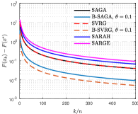
We present a uniform analysis of biased stochastic gradient methods for minimizing convex, strongly convex, and non-convex composite objectives, and identify settings where bias is useful in stochastic gradient estimation. The framework we present allows us to extend proximal support to biased algorithms, including SAG and SARAH, for the first time in the convex setting. We also use our framework to develop a new algorithm, Stochastic Average Recursive GradiEnt (SARGE), that achieves the oracle complexity lower-bound for non-convex, finite-sum objectives and requires strictly fewer calls to a stochastic gradient oracle per iteration than SVRG and SARAH. 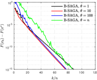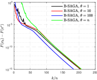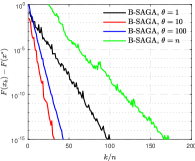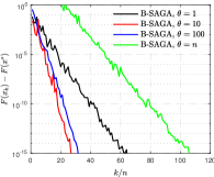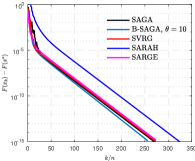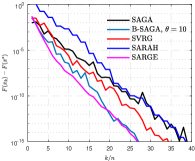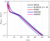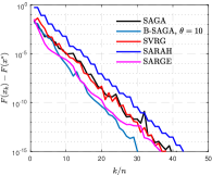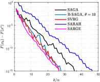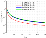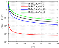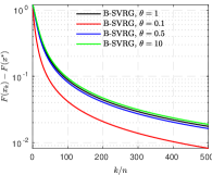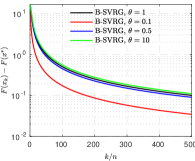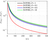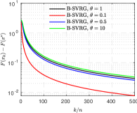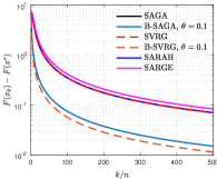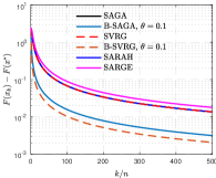We support our theoretical results with numerical experiments that demonstrate the benefits of certain biased gradient estimators.

1 Introduction

In this paper, we focus on the following composite minimisation problem:

$$\min_{x\in\mathbb{R}^{p}}\big{\{}F(x)\stackrel{{\scriptstyle\mathrm{def}}}{{=}}f(x)+g(x)\big{\}}.$$ (1)

Throughout, we assume:

• $g$ is proper and closed such that its proximity operator (see (11) in Section 2) is well posed,

• $f$ admits finite-sum structure $f(x)\stackrel{{\scriptstyle\mathrm{def}}}{{=}}\frac{1}{n}\sum_{i=1}^{n}f_{i}(x)$, and for all $i\in\{1,2,\cdots,n\}$, $\nabla f_{i}$ is $L$-Lipschitz continuous for some $L>0$.

We place no further restrictions on $f_{i}$ or $g$ unless stated otherwise.

Problems of this form arise frequently in many areas of science and engineering, such as machine learning, statistics, operations research, and imaging. For instance, in machine learning, these problems often arise as empirical risk minimisation problems from classification and regression tasks. Examples include ridge regression, logistic regression, Lasso, and $\ell_{1}$-regularized logistic regression [8]. Principal component analysis (PCA) can also be formulated as a problem with this structure, where the functions $f_{i}$ are non-convex [16, 6]. In imaging, $\ell_{1}$ or total variation regularization is often combined with differentiable data discrepancy terms that appear in both convex and non-convex instances [10].

1.1 Stochastic gradient methods

Two classical approaches to solve (1) are the proximal gradient descent method (PGD) [21] and its accelerated variants, including inertial PGD [20] and FISTA [7]. For these deterministic approaches, the full gradient of $f$ must be evaluated at each iteration, which often requires huge computational resources when $n$ is large. Such a drawback makes these schemes unsuitable for large-scale machine learning tasks.

By exploiting the finite sum structure of $f$, stochastic gradient methods enjoy low per-iteration complexity while achieving comparable convergence rates. These qualities make stochastic gradient methods the standard approach to solving many problems in machine learning, and are gaining popularity in other areas such as image processing [11]. Stochastic gradient descent (SGD) was first proposed in the 1950’s [28] and has experienced a renaissance in the past decade, with numerous variants of SGD proposed in the literature (see, for instance, [30, 18, 13] and references therein). Most of these algorithms can be summarised into one general form, which is described below in Algorithm 1.

Algorithm 1 Stochastic gradient descent framework

1:starting point $x_{0}\in\mathbb{R}^{p}$, gradient estimator $\widetilde{\nabla}$.

2:for $k=0,1,\cdots,T-1$ do

3:     Compute stochastic gradient $\widetilde{\nabla}_{k}$ at current iteration $k$.

4:     Choose step size/learning rate $\eta_{k}$.

5:     Update $x_{k+1}$:

$$x_{k+1}\leftarrow\textnormal{prox}_{\eta_{k}g}(x_{k}-\eta_{k}\widetilde{\nabla}_{k}).$$ (2)

6:end for

Below we summarize several popular stochastic gradient estimators $\widetilde{\nabla}_{k}$:

• SGD Classic stochastic gradient descent [28] uses the following gradient estimator at iteration $k$:

  $$\left\lfloor\begin{aligned} &\textrm{sample $j_{k}$ uniformly at random from $\{1,...,n\}$},\\ &\widetilde{\nabla}^{\textnormal{\tiny SGD}}_{k}=\nabla f_{j_{k}}(x_{k}).\end{aligned}\right.$$ (3)

  At each step, SGD uses the gradient of the sampled function $\nabla f_{j_{k}}(x_{k})$ as a stochastic approximation of the full gradient $\nabla f(x_{k})$. It is an unbiased estimate as $\mathbb{E}_{k}[\nabla f_{j_{k}}(x_{k})]=\nabla f(x_{k})$. It is also memoryless: every update of $x_{k+1}$ depends only upon $x_{k}$ and the random variable $j_{k}$. The variance of SGD is does not vanish as $x_{k}$ converges.

• SAG To deal with the non-vanishing variance of SGD, in [29, 30] the authors introduce the SAG gradient estimator, which uses the gradient history to decrease its variance. With $\nabla f_{i}(\varphi^{i}_{0})=0,i=1,...,n$, the SAG gradient estimator is computed using the following procedure:

  $$\left\lfloor\begin{aligned} &\textrm{sample $j_{k}$ uniformly at random from $\{1,...,n\}$},\\ &\widetilde{\nabla}^{\textnormal{\tiny SAG}}_{k}=\tfrac{1}{n}(\nabla f_{j_{k}}(x_{k})-\nabla f_{j_{k}}(\varphi_{k}^{j_{k}}))+\tfrac{1}{n}\mathbin{\scalebox{1.25}{$\sum$}}_{i=1}^{n}\nabla f_{i}(\varphi_{k}^{i}),\\ &\textrm{update the gradient history: $\varphi_{k+1}^{j_{k}}=x_{k}$ and }\nabla f_{i}(\varphi_{k+1}^{i})=\left\{\begin{aligned} &\nabla f_{i}(x_{k})&&\textrm{if\leavevmode\nobreak\ \leavevmode\nobreak\ }i=j_{k},\\ &\nabla f_{i}(\varphi_{k}^{i})&&\textrm{o.w.}\end{aligned}\right.\end{aligned}\right.$$ (4)

  Here, for each $i\in\{1,...,n\}$, $\nabla f_{i}(\varphi_{k}^{i})$ is a stored gradient of $\nabla f_{i}$ from a previous iteration. With the help of memory, the variance of the SAG gradient estimator diminishes as $x_{k}$ approaches the solution; estimators that satisfy this property are known as variance-reduced estimators. In contrast to the SGD estimator, $\widetilde{\nabla}^{\textnormal{\tiny SAG}}_{k}$ is a biased estimate of $\nabla f(x_{k})$.

• SAGA Based on [29, 30], [13] propose the unbiased gradient estimator SAGA, which is computed using the procedure below.

  $$\left\lfloor\begin{aligned} &\textrm{Sample $j_{k}$ uniformly at random from $\{1,...,n\}$},\\ &\widetilde{\nabla}^{\textnormal{\tiny SAGA}}_{k}={\nabla f_{j_{k}}(x_{k})-\nabla f_{j_{k}}(\varphi_{k}^{j_{k}})}+\tfrac{1}{n}\mathbin{\scalebox{1.25}{$\sum$}}_{i=1}^{n}\nabla f_{i}(\varphi_{k}^{i}),\\ &\textrm{update the gradient history: $\varphi_{k+1}^{j_{k}}=x_{k}$ and }\nabla f_{i}(\varphi_{k+1}^{i})=\left\{\begin{aligned} &\nabla f_{i}(x_{k})&&\textrm{if\leavevmode\nobreak\ \leavevmode\nobreak\ }i=j_{k},\\ &\nabla f_{i}(\varphi_{k}^{i})&&\textrm{o.w.}\end{aligned}\right.\end{aligned}\right.$$ (5)

  Compared to $\widetilde{\nabla}^{\textnormal{\tiny SAG}}$, the SAGA estimator gives less weight to stored gradients. With this adjustment, $\widetilde{\nabla}^{\textnormal{\tiny SAGA}}$ is unbiased while maintaining the variance reduction property. Similar gradient estimators can be found in Point-SAGA [12], Finito [14], MISO [22], SDCA [31], and those in [17].

• SVRG Another popular variance-reduced estimator is SVRG [18]. The SVRG gradient estimator is computed as follows:

  $$\left\lfloor\begin{aligned} &\textrm{For $s=0,\dotsm,S$}\\ &\textstyle\nabla f(\varphi_{s})=\tfrac{1}{n}\sum_{i=1}^{n}\nabla f_{i}(\varphi_{s}),\\ &\textrm{For $k=1,\dotsm,m$}\\ &\left\lfloor\begin{aligned} &\textrm{Sample $j_{k}$ uniformly at random from $\{1,\dotsm,n\}$},\\ &\widetilde{\nabla}^{\textnormal{\tiny SVRG}}_{k}=\nabla f_{j_{k}}(x_{k})-\nabla f_{j_{k}}(\varphi_{s})+\nabla f(\varphi_{s}),\\ \end{aligned}\right.\\ \end{aligned}\right.$$ (6)

  where $\varphi_{s}$ is a “snapshot” point updated every $m$ steps. The algorithms prox-SVRG [34], Katyusha [2], KatyushaX [3], Natasha [1], Natasha2 [4], MiG [35], ASVRG [32], and VARAG [19] use the SVRG gradient estimator.

• SARAH In [24] the authors proposed a recursive modification to SVRG.

  $$\left\lfloor\begin{aligned} &\textrm{For $s=0,\dotsm,S$}\\ &\textstyle\widetilde{\nabla}^{\textnormal{\tiny SARAH}}_{k-1}=\tfrac{1}{n}\sum_{i=1}^{n}\nabla f_{i}(\varphi_{s}),\\ &\textrm{For $k=1,\dotsm,m$}\\ &\left\lfloor\begin{aligned} &\textrm{Sample $j_{k}$ uniformly at random from $\{1,\dotsm,n\}$},\\ &\widetilde{\nabla}^{\textnormal{\tiny SARAH}}_{k}=\nabla f_{j_{k}}(x_{k})-\nabla f_{j_{k}}(x_{k-1})+\widetilde{\nabla}^{\textnormal{\tiny SARAH}}_{k-1},\\ \end{aligned}\right.\\ \end{aligned}\right.$$ (7)

  Like SAG, SARAH is a biased gradient estimator. It is also used in prox-SARAH [25], SPIDER [15], SPIDERBoost [33] and SPIDER-M [36].

We refer to algorithms employing (un)biased gradient estimators as (un)biased stochastic algorithms, respectively. The body of work on biased algorithms is stunted compared to the enormous literature on unbiased algorithms, leading to several gaps in the development of biased stochastic gradient methods. We list a few below.

• Complex convergence proofs. It is commonly believed that the relationship $\mathbb{E}_{k}[\widetilde{\nabla}_{k}]=\nabla f(x_{k})$ is essential for a simple convergence analysis (see, for example, the discussion in [13]). The convergence proof of the biased algorithm SAG is especially complex, requiring computational verification [29, 30].

• Sub-optimal convergence rates. In the convex setting with $g\equiv 0$, SARAH achieves a complexity bound of $\mathcal{O}(\frac{\log(1/\epsilon)}{\epsilon})$ [24] for finding a point $\bar{x}_{k}$ such that $\mathbb{E}[F(\bar{x}_{k})-F(x^{\star})]\leq\epsilon$. In comparison, SAGA and SVRG achieve a complexity bound of $\mathcal{O}(1/\epsilon)$ which is the same as deterministic proximal gradient descent.

• Lack of proximal support. Bias also makes it difficult to handle non-smooth functions. To the best of our knowledge, there are no theoretical guarantees for biased algorithms to solve (1) with $g\not\equiv 0$ that take advantage of convexity when it is present.

Despite the above shortcomings, there are notable exceptions that suggest biased algorithms are worth further consideration. Recently, [25, 15, 33, 36] proved that algorithms using the SARAH gradient estimator require $\mathcal{O}(\sqrt{n}/\epsilon^{2})$ stochastic gradient evaluations to find an $\epsilon$-first order stationary point. This matches the complexity lower-bound for non-convex, finite-sum optimisation for smooth functions $f_{i}$ and $n\leq\mathcal{O}(\epsilon^{-4})$ [15]. For comparison, the best complexity bound obtained for SAGA and SVRG in this setting is $\mathcal{O}(n^{2/3}/\epsilon^{2})$ [26, 5]. A detailed summary of existing complexity bounds for the variance-reduced gradient estimators mentioned above is provided in Table 1 for convex, strongly convex and non-convex settings.

	Convex	Strongly Convex	Non-Convex	Proximal Support?
SAGA	$\mathcal{O}(\frac{nL}{\epsilon})$	$\mathcal{O}((n+\kappa)\log(1/\epsilon))$	$\mathcal{O}(\frac{nL}{\epsilon^{2}})^{b}$	Yes
SVRG	$\mathcal{O}(\frac{nL}{\epsilon})$	$\mathcal{O}((n+\kappa)\log(1/\epsilon))$	$\mathcal{O}(\frac{nL}{\epsilon^{2}})$	Yes
SAG	$\mathcal{O}(\frac{nL}{\epsilon})$	$\mathcal{O}((n+\kappa)\log(1/\epsilon))$	Unknown	No
SARAH	$\mathcal{O}(\frac{L\log(1/\epsilon)}{\epsilon})$	$\mathcal{O}((n+\kappa)\log(1/\epsilon))$	$\mathcal{O}(\frac{\sqrt{n}L}{\epsilon^{2}})$	Non-Convex Only

Table 1: Existing complexity bounds for stochastic gradient estimators under different settings. These complexities represent the number of stochastic gradient oracle calls required to find a point satisfying $\mathbb{E}[F(\bar{x}_{k})-F(x^{\star})]\leq\epsilon$ for the convex case, $\mathbb{E}[\|x_{k}-x^{\star}\|^{2}]\leq\epsilon$ for the strongly convex case, and an $\epsilon$-approximate stationary point (as in Definition 1) in the non-convex case. In the strongly convex case, $\mu$ is the strong convexity constant, and $\kappa=L/\mu$ is the condition number.

1.2 Contributions

This work provides three main contributions:

1. We introduce a framework for the systematic analysis of a large class of stochastic gradient methods and investigate a bias-variance tradeoff arising from our analysis. Our analysis provides proximal support to biased algorithms for the first time in the convex setting.

2. We apply our framework to derive convergence rates for SARAH and biased versions of SAGA and SVRG on convex, strongly convex, and non-convex problems.

3. We design a new recursive gradient estimator, Stochastic Average Recursive GradiEnt (SARGE), that achieves the same convergence rates as SARAH but never computes a full gradient, giving it a strictly smaller per-iteration complexity than SARAH. In particular, we show that SARGE achieves the oracle complexity lower bound for non-convex finite-sum optimisation.

To study the effects of bias on the SAGA and SVRG estimators, we introduce Biased SAGA (B-SAGA) and Biased SVRG (B-SVRG). For $\theta>0$ the B-SAGA and B-SVRG gradient estimators are

• B-SAGA:

  $$\widetilde{\nabla}^{\textnormal{\tiny B-SAGA}}_{k}\stackrel{{\scriptstyle\mathrm{def}}}{{=}}\tfrac{1}{\theta}(\nabla f_{j_{k}}(x_{k})-\nabla f_{j_{k}}(\varphi_{k}^{j_{k}}))+\tfrac{1}{n}\mathbin{\scalebox{1.25}{$\sum$}}_{i=1}^{n}\nabla f_{i}(\varphi_{k}^{i}),$$ (8)

• B-SVRG:

  $$\widetilde{\nabla}^{\textnormal{\tiny B-SVRG}}_{k}\stackrel{{\scriptstyle\mathrm{def}}}{{=}}\tfrac{1}{\theta}(\nabla f_{j_{k}}(x_{k})-\nabla f_{j_{k}}(\varphi_{s}))+\nabla f(\varphi_{s}).$$ (9)

In both B-SAGA and B-SVRG, the bias parameter $\theta$ adjusts how much weight is given to stored gradient information. When $\theta=n$, $\widetilde{\nabla}^{\textnormal{\tiny B-SAGA}}_{k}$ recovers the SAG gradient estimator.

Motivated by the desirable properties of SARAH, we propose a new gradient estimator, Stochastic Average Recursive GradiEnt (SARGE), which is defined below

$$\widetilde{\nabla}^{\textnormal{\tiny SARGE}}_{k}\stackrel{{\scriptstyle\mathrm{def}}}{{=}}\nabla f_{j_{k}}(x_{k})-\psi_{k}^{j_{k}}+\tfrac{1}{n}\mathbin{\scalebox{1.25}{$\sum$}}_{i=1}^{n}\psi_{k}^{i}-(1-\tfrac{1}{n})(\nabla f_{j_{k}}(x_{k-1})-\widetilde{\nabla}^{\textnormal{\tiny SARGE}}_{k-1}),$$ (10)

where the variables $\psi_{k}^{i}$ follow the update rule $\psi_{k+1}^{i_{k}}=\nabla f_{j_{k}}(x_{k})-(1-\tfrac{1}{n})\nabla f_{j_{k}}(x_{k-1})$. Similar to SAGA, SARGE uses stored gradient information to avoid having to compute the full gradient, a computational burden that SVRG and SARAH require for variance reduction.

A summary of the complexity results obtained from our analysis for SAG/B-SAGA, B-SVRG, SARAH, and SARGE are provided in Table 2. Note that the result for SAG is included in B-SAGA.

	Convex	Strongly Convex	Non-Convex	Proximal Support?
B-SAGA	$\mathcal{O}(\frac{nL}{\epsilon})$	$\mathcal{O}(n\kappa\log(1/\epsilon))$	$\mathcal{O}(\frac{nL}{\epsilon^{2}})$	Yes
B-SVRGc	$\mathcal{O}(\frac{nL}{\epsilon})$	$\mathcal{O}(n\kappa\log(1/\epsilon))$	$\mathcal{O}(\frac{nL}{\epsilon^{2}})$	Yes
SARAH	$\mathcal{O}(\frac{\sqrt{n}L}{\epsilon})$	$\mathcal{O}(\max\{\sqrt{n}\kappa,n\}\log(1/\epsilon))$	$\mathcal{O}(\frac{\sqrt{n}L}{\epsilon^{2}})$	Yes
SARGE	$\mathcal{O}(\frac{\sqrt{n}L}{\epsilon})$	$\mathcal{O}(\max\{\sqrt{n}\kappa,n\}\log(1/\epsilon))$	$\mathcal{O}(\frac{\sqrt{n}L}{\epsilon^{2}})$	Yes

Table 2: Complexity bounds obtained from our analysis framework. These complexities represent the number of stochastic gradient oracle calls required to find a point $\bar{x}_{k}$ satisfying $\mathbb{E}[F(\bar{x}_{k})-F(x^{\star})]\leq\epsilon$ for the convex case, $\mathbb{E}[\|x_{k}-x^{\star}\|^{2}]\leq\epsilon$ for the strongly convex case, and an $\epsilon$-approximate stationary point in the non-convex case.

Paper organization

Preliminary results and notations are provided in Section 2. A discussion on the tradeoff between bias and variance in stochastic optimisation is included in Section 3. Our main convergence results are presented in Section 4. In Section 5, we substantiate our theoretical results using numerical experiments involving several classic regression tasks arising from machine learning. All the proofs of the main results are collected in the appendix.

2 Preliminaries and notations

Throughout the paper, $\mathbb{R}^{p}$ is a $p$-dimensional Euclidean space equipped with scalar inner product $\langle\cdot,\,\cdot\rangle$ and associated norm ${|\kern-1.125pt|}\cdot{|\kern-1.125pt|}$. The sub-differential of a proper closed convex function $g$ is the set-valued operator defined by $\partial g\stackrel{{\scriptstyle\mathrm{def}}}{{=}}\big{\{}v\in\mathbb{R}^{n}|g(x^{\prime})\geq g(x)+\langle v,\,x^{\prime}-x\rangle,\forall x^{\prime}\in\mathbb{R}^{n}\big{\}}$, the proximal map of $g$ is defined as

$$\textstyle\textnormal{prox}_{\eta g}(y)\stackrel{{\scriptstyle\mathrm{def}}}{{=}}\operatorname*{arg\,min}_{x\in\mathbb{R}^{n}}\eta g(x)+\tfrac{1}{2}{|\kern-1.125pt|}x-y{|\kern-1.125pt|}^{2},$$ (11)

where $\eta>0$ and $y\in\mathbb{R}^{p}$. With $y^{+}=\textnormal{prox}_{\gamma g}(y)$, (11) is equivalent to $y-y^{+}\in\eta\partial g(y^{+})$.

Below we summarize some useful results in convex analysis.

Lemma 1 ([23, Thm 2.1.5])

Suppose $f$ is convex with an $L$-Lipschitz continuous gradient. We have for every $x,u\in\mathbb{R}^{p}$,

$$\|\nabla f(x)-\nabla f(u)\|^{2}\leq 2L(f(x)-f(u)-\langle\nabla f(u),x-u\rangle).$$ (12)

When $f$ is a finite sum as in (1), Lemma 1 is equivalent to the following result.

Lemma 2

Let $f(x)=\tfrac{1}{n}\sum_{i=1}^{n}f_{i}(x)$, where each $f_{i}$ is convex with an $L$-Lipschitz gradient. Then for every $x,u\in\mathbb{R}^{p}$,

$$\textstyle\tfrac{1}{2Ln}\sum_{i=1}^{n}\|\nabla f_{i}(x)-\nabla f_{i}(u)\|^{2}\leq f(x)-f(u)-\langle\nabla f(u),x-u\rangle.$$ (13)

Lemma 2 is obtained by applying Lemma 1 to each $f_{i}$ and averaging.

Lemma 3

Suppose $g$ is $\mu$-strongly convex with $\mu\geq 0$, and let $z=\textnormal{prox}_{\eta g}(x-\eta d)$ for some $x,d\in\mathbb{R}^{p}$ and $\eta>0$. Then, for any $y\in\mathbb{R}^{p}$,

$$\textstyle\eta\langle d,z-y\rangle\leq\tfrac{1}{2}\|x-y\|^{2}-\tfrac{1+\mu\eta}{2}\|z-y\|^{2}-\tfrac{1}{2}\|z-x\|^{2}-\eta g(z)+\eta g(y).$$ (14)

Proof.

By the strong convexity of $g$,

$$g(z)-g(y)\leq\langle\xi,z-y\rangle-\tfrac{\mu}{2}\|z-y\|^{2},\quad\forall\xi\in\partial g(z).$$ (15)

From the definition of the proximal operator, we have that $\frac{1}{\eta}(x-z)-d\in\partial g(z)$. Therefore,

$$\textstyle g(z)-g(y) \textstyle\leq\langle\xi,z-y\rangle-\tfrac{\mu}{2}\|z-y\|^{2}$$ (16)

$$=\textstyle\tfrac{1}{\eta}\langle x-z-\eta d,z-y\rangle-\tfrac{\mu}{2}\|z-y\|^{2}$$

$$=\textstyle-\langle d,\,z-y\rangle+\tfrac{1}{\eta}\langle x-z,\,z-y\rangle-\tfrac{\mu}{2}\|z-y\|^{2}$$

$$=\textstyle-\langle d,\,z-y\rangle-\tfrac{1}{2\eta}{|\kern-1.125pt|}x-z{|\kern-1.125pt|}^{2}-\tfrac{1}{2\eta}{|\kern-1.125pt|}z-y{|\kern-1.125pt|}^{2}+\tfrac{1}{2\eta}{|\kern-1.125pt|}x-y{|\kern-1.125pt|}^{2}-\tfrac{\mu}{2}\|z-y\|^{2}.$$

Multiplying by $\eta$ and rearranging yields the assertion. ∎

The next lemma is an analogue of the descent lemma for gradient descent when the gradient is replaced with an arbitrary vector $d$.

Lemma 4

Suppose $g$ is $\mu$-strongly convex for $\mu\geq 0$, and let $z=\textnormal{prox}_{\eta g}(x-\eta d)$. The following inequality holds for any $\lambda>0$.

$$\textstyle 0\leq\eta(F(x)-F(z))+\tfrac{\eta}{2L\lambda}\|d-\nabla f(x)\|^{2}+(\tfrac{\eta L(\lambda+1)}{2}-\tfrac{2+\mu\eta}{2})\|z-x\|^{2}.$$ (17)

Proof.

This follows immediately from Lemma 3.

$$\textstyle 0 \textstyle=\eta\langle d,x-z\rangle+\eta\langle d,z-x\rangle$$ (18)

$$\textstyle\stackrel{{\scriptstyle\mathclap{\raisebox{0.5pt}{\footnotesize\raisebox{-.9pt} {1}⃝}}}}{{\leq}}\eta\langle d,x-z\rangle-\tfrac{2+\mu\eta}{2}\|z-x\|^{2}+\eta(g(x)-g(z))$$

$$\textstyle=\eta\langle\nabla f(x),x-z\rangle+\eta\langle d-\nabla f(x),x-z\rangle-\tfrac{2+\mu\eta}{2}\|z-x\|^{2}+\eta(g(x)-g(z))$$

$$\textstyle\stackrel{{\scriptstyle\mathclap{\raisebox{0.5pt}{\footnotesize\raisebox{-.9pt} {2}⃝}}}}{{\leq}}\eta(F(x)-F(z))+\eta\langle d-\nabla f(x),x-z\rangle+(\tfrac{\eta L}{2}-\tfrac{2+\mu\eta}{2})\|z-x\|^{2}$$

$$\textstyle\stackrel{{\scriptstyle\mathclap{\raisebox{0.5pt}{\footnotesize\raisebox{-.9pt} {3}⃝}}}}{{\leq}}\eta(F(x)-F(z))+\tfrac{\eta}{2L\lambda}\|d-\nabla f(x)\|^{2}+(\tfrac{\eta L(\lambda+1)}{2}-\tfrac{2+\mu\eta}{2})\|z-x\|^{2}.$$

Inequality \raisebox{-.9pt} {1}⃝ is due to Lemma 3 with $y=x$, \raisebox{-.9pt} {2}⃝ is due to the Lipschitz continuity of $\nabla f_{i}$, and \raisebox{-.9pt} {3}⃝ is Young’s. ∎

The previous two lemmas require $g$ to be convex. Similar results hold in the non-convex case as well.

Lemma 5

Let $z=\textnormal{prox}_{\eta g}(x-\eta d)$ for some $x,d\in\mathbb{R}^{p}$ and $\eta>0$. Then, for any $y\in\mathbb{R}^{p}$,

$$\textstyle\eta\langle d,z-y\rangle\leq\tfrac{1}{2}\|x-y\|^{2}-\tfrac{1}{2}\|z-x\|^{2}-\eta g(z)+\eta g(y).$$ (19)

Proof.

By the Lipschitz continuity of $\nabla f$, we have the inequalities

$$f(x)-f(y) \textstyle\leq\langle\nabla f(x),x-y\rangle+\frac{L}{2}\|x-y\|^{2},$$ (20)

$$f(z)-f(x) \textstyle\leq\langle\nabla f(x),z-x\rangle+\frac{L}{2}\|z-x\|^{2}.$$

Furthermore, by the definition of $z$,

$$z\in\operatorname*{arg\,min}_{v}\left\{\langle d,v-x\rangle+\frac{1}{2\eta}\|v-x\|^{2}+g(v)\right\}.$$ (21)

Taking $v=y$, we obtain

$$\textstyle g(z)-g(y)\leq\langle d,y-z\rangle+\frac{1}{2\eta}\left(\|x-y\|^{2}-\|x-z\|^{2}\right).$$ (22)

Adding these three inequalities and multiplying by $\eta$ completes the proof. ∎

Lemma 6

Let $z=\textnormal{prox}_{\eta g}(x-\eta d)$. Then

$$\textstyle F(z)\leq F(y)+\langle\nabla f(x)-d,z-y\rangle+(\frac{L}{2}-\frac{1}{2\eta})\|x-z\|^{2}+(\frac{L}{2}+\frac{1}{2\eta})\|x-y\|^{2}.$$ (23)

Proof.

By the Lipschitz continuity of $\nabla f$, we have the inequalities

$$f(x)-f(y) \textstyle\leq\langle\nabla f(x),x-y\rangle+\frac{L}{2}\|x-y\|^{2},$$ (24)

$$f(z)-f(x) \textstyle\leq\langle\nabla f(x),z-x\rangle+\frac{L}{2}\|z-x\|^{2}.$$

Furthermore, by Lemma 5,

$$\textstyle g(z)-g(y)\leq\langle d,y-z\rangle+\frac{1}{2\eta}\left(\|x-y\|^{2}-\|x-z\|^{2}\right).$$ (25)

Adding these inequalities together completes the proof. ∎

In the non-convex setting, to measure convergence of the sequence to a first-order stationary point, we use the notion of a generalized gradient [23].

Definition 1 (Generalized gradient map)

The generalized gradient map is defined as

$$\textstyle\mathcal{G}_{\eta_{k}}(x_{k})\stackrel{{\scriptstyle\mathrm{def}}}{{=}}\tfrac{1}{\eta_{k}}(x_{k}-\textnormal{prox}_{\eta_{k}g}(x_{k}-\eta_{k}\nabla f(x_{k}))).$$

When $g\equiv 0$, we have $\mathcal{G}_{\eta_{k}}(x_{k})=\nabla f(x_{k})\to 0$ if the sequence $\{x_{k}\}$ converges to some $x^{\star}\in\mathbb{R}^{p}$ such that $\nabla f(x^{\star})=0$. For nontrivial $g$, suppose $\inf_{k}\eta_{k}>0$ and $x_{k}$ converges to some $x^{\star}$ such that $x^{\star}=\textnormal{prox}_{\eta g}(x^{\star}-\eta\nabla f(x^{\star}))$, then $\mathcal{G}_{\eta_{k}}(x)\to 0$. Such a point $x^{\star}$ is called first-order stationary point of (1) and an $\epsilon$-first-order stationary point is a point satisfying $\|\mathcal{G}_{\eta}(x)\|\leq\epsilon$ for some $\eta>0$.

3 A bias-variance tradeoff in stochastic gradient methods

In this section, we discuss the effect of the bias and variance of a stochastic gradient estimator on the performance of Algorithm 1. It is elementary that the mean-squared error (MSE) of a stochastic estimator can be decomposed into the sum of its variance and squared bias. In our setting,

$$\mathbb{E}_{k}[\|\widetilde{\nabla}_{k}-\nabla f(x_{k})\|^{2}]=\|\mathbb{E}_{k}[\widetilde{\nabla}_{k}]-\nabla f(x_{k})\|^{2}+\mathbb{E}_{k}[\|\widetilde{\nabla}_{k}-\mathbb{E}_{k}[\widetilde{\nabla}_{k}]\|^{2}].$$ (26)

This decomposition shows that a biased estimator might have a smaller MSE than an unbiased estimator as long as the bias sufficiently diminishes the variance. This is the bias-variance tradeoff. As we see below, a bias-variance tradeoff exists in our analysis of stochastic gradient methods, but with a slightly different form.

In what follows, we first discuss the bias-variance tradeoff in the convex settings and then the non-convex setting.

3.1 Convex case

Let $x^{\star}$ be a global minimizer of problem (1). From the update (2), let $w_{k+1}\in\partial g(x_{k+1})$. We have the following bound on the suboptimality at $x_{k+1}$:

$$\mathbb{E}_{k}[F(x_{k+1})-F(x^{\star})]$$ (27)

$$=\mathbb{E}_{k}[f(x_{k+1})-f(x_{k})+f(x_{k})-f(x^{\star})+g(x_{k+1})-g(x^{\star})]$$

$$\stackrel{{\scriptstyle\mathclap{\raisebox{0.5pt}{\footnotesize\raisebox{-.9pt} {1}⃝}}}}{{\leq}}\tfrac{L}{2}\mathbb{E}_{k}[\|x_{k+1}-x_{k}\|^{2}]+\mathbb{E}_{k}[\langle\nabla f(x_{k}),x_{k+1}-x_{k}\rangle]+\langle\nabla f(x_{k}),x_{k}-x^{\star}\rangle+\mathbb{E}_{k}[g(x_{k+1})-g(x^{\star})]$$

$$=\tfrac{L}{2}\mathbb{E}_{k}[\|x_{k+1}-x_{k}\|^{2}]+\mathbb{E}_{k}[\langle\nabla f(x_{k})-\widetilde{\nabla}_{k},x_{k+1}-x_{k}\rangle]$$

$$\qquad+\mathbb{E}_{k}[\langle\nabla f(x_{k})-\widetilde{\nabla}_{k},x_{k}-x^{\star}\rangle]+\mathbb{E}_{k}[\langle\widetilde{\nabla}_{k},x_{k+1}-x^{\star}\rangle]+\mathbb{E}_{k}[g(x_{k+1})-g(x^{\star})]$$

$$\stackrel{{\scriptstyle\mathclap{\raisebox{0.5pt}{\footnotesize\raisebox{-.9pt} {2}⃝}}}}{{\leq}}\tfrac{\epsilon}{2}\mathbb{E}_{k}[\|\nabla f(x_{k})-\widetilde{\nabla}_{k}\|^{2}]+(\tfrac{L}{2}+\tfrac{1}{2\epsilon})\mathbb{E}_{k}[\|x_{k+1}-x_{k}\|^{2}]$$

$$\qquad+\mathbb{E}_{k}[\langle\nabla f(x_{k})-\widetilde{\nabla}_{k},x_{k}-x^{\star}\rangle]+\mathbb{E}_{k}[\langle\widetilde{\nabla}_{k}+w_{k+1},x_{k+1}-x^{\star}\rangle-\tfrac{\mu}{2}\|x_{k+1}-x^{*}\|^{2}]$$

$$\stackrel{{\scriptstyle\mathclap{\raisebox{0.5pt}{\footnotesize\raisebox{-.9pt} {3}⃝}}}}{{\leq}}\tfrac{\epsilon}{2}\mathbb{E}_{k}[\|\nabla f(x_{k})-\widetilde{\nabla}_{k}\|^{2}]+(\tfrac{L}{2}+\tfrac{1}{2\epsilon}-\tfrac{1}{2\eta})\mathbb{E}_{k}[\|x_{k+1}-x_{k}\|^{2}]$$

$$\qquad+\mathbb{E}_{k}[\langle\nabla f(x_{k})-\widetilde{\nabla}_{k},x_{k}-x^{\star}\rangle]-\tfrac{1+\mu\eta}{2\eta}\mathbb{E}_{k}[\|x_{k+1}-x^{\star}\|^{2}]+\tfrac{1}{2\eta}{\|x_{k}-x^{\star}\|^{2}}.$$

Inequality \raisebox{-.9pt} {1}⃝ follows from the convexity of $f$ and Lipschitz continuity of $\nabla f$, \raisebox{-.9pt} {2}⃝ follows from the (strong) convexity of $g$, and \raisebox{-.9pt} {3}⃝ comes from the implicit definition of the proximal operator (11). For the last line of the inequality, we observe that the inner product term $\mathbb{E}_{k}[\langle\nabla f(x_{k})-\widetilde{\nabla}_{k},\,x_{k}-x^{\star}\rangle]$ vanishes when $\widetilde{\nabla}_{k}$ is an unbiased estimate of $\nabla f(x_{k})$. When the estimator is biased, we must develop a new way to control this term, together with $\mathbb{E}_{k}[{|\kern-1.125pt|}\nabla f(x_{k})-\widetilde{\nabla}_{k}{|\kern-1.125pt|}^{2}]$.

Hence, the following terms arise in our convergence analysis from the bias and the variance of the gradient estimator:

Bias $$:\mathbb{E}_{k}[\langle\nabla f(x_{k})-\widetilde{\nabla}_{k},\,x_{k}-x^{\star}\rangle]\enskip\textrm{and}\enskip\|\mathbb{E}_{k}[\widetilde{\nabla}_{k}]-\nabla f(x_{k})\|^{2},$$ (28)

Variance $$:\mathbb{E}_{k}[\|\widetilde{\nabla}_{k}-\mathbb{E}_{k}[\widetilde{\nabla}_{k}]\|^{2}].$$

Remark 1 (Non-composite case ${g=0}$)

When $g=0$, for gradient descent, the descent property of $f$ yields

$$f(x_{k+1})-f(x^{\star}) \leq(\tfrac{L}{2}-\tfrac{1}{\eta})\|x_{k+1}-x_{k}\|^{2}+f(x_{k})-f(x^{\star}),$$ (29)

where $\eta\leq 2/L$. For stochastic gradient descent, we obtain the following relationship:

$$\mathbb{E}_{k}[f(x_{k+1})-f(x^{\star})]$$ (30)

$$=\mathbb{E}_{k}[f(x_{k+1})-f(x_{k})+f(x_{k})-f(x^{\star})]$$

$$\leq\mathbb{E}_{k}[\langle\nabla f(x_{k})-{\widetilde{\nabla}_{k}},x_{k+1}-x_{k}\rangle]+(\tfrac{L}{2}-\tfrac{1}{\eta})\mathbb{E}_{k}[\|x_{k+1}-x_{k}\|^{2}]+f(x_{k})-f(x^{\star})$$

$$\leq\tfrac{\epsilon}{2}\mathbb{E}_{k}[\|\nabla f(x_{k})-\widetilde{\nabla}_{k}\|^{2}]+(\tfrac{L}{2}+\tfrac{1}{2\epsilon}-\tfrac{1}{\eta})\mathbb{E}_{k}[\|x_{k+1}-x_{k}\|^{2}]+f(x_{k})-f(x^{\star}).$$

Compared to (27), there is no inner product term in (30), which makes the analysis of the non-composite case much simpler. This is one reason why biased algorithms have been successfully studied in non-composite setting, but not in the composite setting.

3.2 Non-convex case

The influence of bias is simpler in the non-convex setting and independent of $g$, which explains why biased algorithms have recently found success for these problems. To begin, let $\hat{x}_{k+1}\stackrel{{\scriptstyle\mathrm{def}}}{{=}}\textnormal{prox}_{\eta/2g}(x_{k}-\eta/2\nabla f(x_{k}))$. Applying Lemma 6 with $z=\hat{x}_{k+1}$, $y=x=x_{k}$ and $d=\nabla f(x_{k})$, we have

$$\textstyle F(\hat{x}_{k+1})\leq F(x_{k})+(\frac{L}{2}-\frac{1}{\eta})\|\hat{x}_{k+1}-x_{k}\|^{2}.$$ (31)

Again, applying Lemma 6 with $z=x_{k+1}$, $y=\hat{x}_{k+1}$, $x=x_{k}$, and $d=\widetilde{\nabla}_{k}$, we obtain

$$F(x_{k+1}) \leq\textstyle F(\hat{x}_{k+1})+\langle\nabla f(x_{k})-\widetilde{\nabla}_{k},x_{k+1}-\hat{x}_{k+1}\rangle+(\frac{L}{2}-\frac{1}{2\eta})\|x_{k+1}-x_{k}\|^{2}$$ (32)

$$\textstyle\qquad+(\frac{L}{2}+\frac{1}{2\eta})\|\hat{x}_{k+1}-x_{k}\|^{2}$$

Adding these two inequalities together gives

$$F(x_{k+1}) \leq F(x_{k})+(L-\tfrac{1}{2\eta})\|\hat{x}_{k+1}-x_{k}\|^{2}+(\tfrac{L}{2}-\tfrac{1}{2\eta})\|x_{k+1}-x_{k}\|^{2}$$ (33)

$$\qquad+\langle\nabla f(x_{k})-\widetilde{\nabla}_{k},x_{k+1}-\hat{x}_{k+1}\rangle$$

$$\stackrel{{\scriptstyle\mathclap{\raisebox{0.5pt}{\footnotesize\raisebox{-.9pt} {1}⃝}}}}{{\leq}}F(x_{k})+(L-\tfrac{1}{2\eta})\|\hat{x}_{k+1}-x_{k}\|^{2}+(\tfrac{L}{2}-\tfrac{1}{2\eta})\|x_{k+1}-x_{k}\|^{2}+2\eta\|\nabla f(x_{k})-\widetilde{\nabla}_{k}\|^{2}$$

$$\quad+\frac{1}{8\eta}\|\hat{x}_{k+1}-x_{k+1}\|^{2}$$

$$\stackrel{{\scriptstyle\mathclap{\raisebox{0.5pt}{\footnotesize\raisebox{-.9pt} {2}⃝}}}}{{\leq}}F(x_{k})+(L-\tfrac{1}{4\eta})\|\hat{x}_{k+1}-x_{k}\|^{2}+(\tfrac{L}{2}-\tfrac{1}{4\eta})\|x_{k+1}-x_{k}\|^{2}+2\eta\|\nabla f(x_{k})-\widetilde{\nabla}_{k}\|^{2}.$$

Inequality \raisebox{-.9pt} {1}⃝ is Young’s, and \raisebox{-.9pt} {2}⃝ is the standard inequality $\|a-c\|^{2}\leq 2\|a-b\|^{2}+2\|b-c\|^{2}$. In the non-convex case, the inner-product bias term does not appear, so the bias-variance tradeoff is the classical one.

3.3 General bounds on bias and variance

To ensure convergence for a particular gradient estimator used in Algorithm 1, we must bound the inner-product bias term $\mathbb{E}_{k}[\langle\nabla f(x_{k})-\widetilde{\nabla}_{k},x_{k}-x^{\star}\rangle]$ and the MSE $\mathbb{E}_{k}[\|\nabla f(x_{k})-\widetilde{\nabla}_{k}\|^{2}]$. Below we introduce general bounds on these terms that allow us to establish convergence rates for a variety of gradient estimators. The first of these is a bound on the MSE term.

Definition 2 (Bounded MSE)

The stochastic gradient estimator $\widetilde{\nabla}$ is said to satisfy the BMSE$(M_{1},M_{2},\rho_{M},$ $\rho_{F},m)$ property with parameters $M_{1},M_{2}\geq 0$, $\rho_{M},\rho_{F}\in(0,1]$ and $m\geq 1$ if there exist sequences $\mathcal{M}_{k}$ and $\mathcal{F}_{k}$ such that

$$\sum_{k=ms}^{m(s+1)-1}\mathbb{E}[\|\widetilde{\nabla}_{k}-\nabla f(x_{k})\|^{2}]\leq\mathcal{M}_{ms},$$ (34)

and the following bounds hold:

$$\mathcal{M}_{ms} \leq(1-\rho_{M})^{m}\mathcal{M}_{m(s-1)}+\mathcal{F}_{ms}+\tfrac{M_{1}}{n}\sum_{k=ms}^{m(s+1)-1}\sum_{i=1}^{n}\mathbb{E}[\|\nabla f_{i}(x_{k+1})-\nabla f_{i}(x_{k})\|^{2}],$$ (35)

$$\mathcal{F}_{ms} \leq\sum_{\ell=0}^{s}\tfrac{M_{2}(1-\rho_{F})^{m(s-\ell)}}{n}\sum_{k=ms}^{m(s+1)-1}\sum_{i=1}^{n}\mathbb{E}[\|\nabla f_{i}(x_{k+1})-\nabla f_{i}(x_{k})\|^{2}].$$

The constant $m$ is the epoch length of the gradient estimator, hence it is usually set to be $\mathcal{O}(n)$. The BMSE property allows these bounds to hold only on average over an epoch. This property is useful in convergence analyses because it bounds the MSE by a geometrically decaying sequence $\{\mathcal{M}_{mk}\}_{k\in\mathbb{N}}$ and a component that is proportional to the one-iteration progress of gradient descent $(1/n\sum_{i=1}^{n}\|\nabla f_{i}(x_{k+1})-\nabla f_{i}(x_{k})\|^{2})$.

Remark 2

  

• Most variance-reduced stochastic gradient estimators satisfy the BMSE property, including SAG, SAGA, SVRG, SARAH, and all the estimators in [17]. SGD does not satisfy this property, as its variance does not decay along the iterations.

• Most existing work on the analysis of general stochastic gradient algorithms enforce bounds of this form on either the MSE or the moments of the stochastic estimator, with the crucial difference that existing works require the bounds to (i.e., dependent on only the previous iteration) [9]. In contrast, the BMSE property allows non-Markovian MSE bounds through the sequence $\mathcal{F}_{k}$. This relaxation is crucial for the analysis of our new gradient estimator, SARGE.

In order to bound the inner-product bias term, we require the gradient estimator to admit a certain structure in its bias. In biased estimators such as SAG, the bias depends on the stored gradient values:

$$\textstyle\nabla f(x_{k})-\mathbb{E}_{k}[\widetilde{\nabla}^{\textnormal{\tiny SAG}}_{k}]=(1-\tfrac{1}{n})\big{(}{\nabla f(x_{k})-\tfrac{1}{n}\sum_{i=1}^{n}\nabla f_{i}(\varphi_{k}^{i})}\big{)}.$$ (36)

We call estimators whose bias admits the above structure memory-biased gradient estimators. These include SAG, and more generally B-SAGA and B-SVRG.

Definition 3 (Memory-biased gradient estimator)

The stochastic gradient estimator $\widetilde{\nabla}$ is memory-biased with parameters $\theta>0$, $B_{1}\geq 0$, and $m\geq 1$ if

$$\nabla f(x_{k})-\mathbb{E}_{k}[\widetilde{\nabla}_{k}]=(1-\tfrac{1}{\theta}){\Big{(}}{\nabla f(x_{k})-{{\frac{\raisebox{-1.75003pt}{\footnotesize$1$}}{\raisebox{1.75003pt}{\footnotesize$n$}}}}\sum_{i=1}^{n}\nabla f_{i}(\varphi_{k}^{i})}{\Big{)}},$$ (37)

for some $\{\varphi_{k}^{i}\}_{i=1}^{n}\subset\{x_{\ell}\}_{\ell=0}^{k-1}$, and for any $s\in\mathbb{N}_{0}$,

$$\sum_{k=ms}^{m(s+1)-1}\tfrac{1}{n}\sum_{i=1}^{n}\mathbb{E}[\|x_{k}-\varphi_{k}^{i}\|^{2}]\leq B_{1}\sum_{k=ms}^{m(s+1)-1}\mathbb{E}[\|x_{k}-x_{k-1}\|^{2}].$$ (38)

B-SAGA is clearly a memory-biased estimator, and so is B-SVRG where $\varphi_{k}^{i}=\varphi_{ms}^{i}$ for all $k$ in epoch $s$. The parameter $\theta$ controls the amount of bias in the estimator, and $B_{1}$, in a sense, measures how “stale” the stored gradient information is. For memory-biased gradient estimators, the bias-term can be handled easily.

Lemma 7

Suppose $\widetilde{\nabla}$ is memory-biased with parameter $\theta\geq 1$ and that $F$ is $\mu$-strongly convex with $\mu\geq 0$. For any $\lambda>0$, the following inequality holds:

$$\eta\mathbb{E}_{k}[F(x_{k+1})-F(x^{\star})] \leq\tfrac{\eta}{2L\lambda}\mathbb{E}_{k}[\|\widetilde{\nabla}_{k}-\nabla f(x_{k})\|^{2}]-\tfrac{1+\mu\eta}{2}\mathbb{E}_{k}[\|x_{k+1}-x^{\star}\|^{2}]+\tfrac{1}{2}\|x_{k}-x^{\star}\|^{2}$$ (39)

$$\qquad+(\tfrac{\eta L(\lambda+1)}{2}-\tfrac{1}{2})\mathbb{E}_{k}[\|x_{k+1}-x_{k}\|^{2}]+\tfrac{\eta L}{2n}(1-\tfrac{1}{\theta})\sum_{i=1}^{n}\|x_{k}-\varphi_{k}^{i}\|^{2}.$$

The proof of Lemma 7 can be found in Appendix A. The bound of Lemma 7 is analogous to the bound in (27), but the inner-product bias term is replaced with $\tfrac{\eta L}{2n}(1-\tfrac{1}{\theta})\sum_{i=1}^{n}\|x_{k}-\varphi_{k}^{i}\|^{2}$. This term is proportional to the progress of gradient descent (by (38)), so this provides the necessary control over the inner-product bias term.

For estimators such as SARAH, the bias depends on the error in the previous gradient estimate, rather than previous stochastic gradients:

$$\nabla f(x_{k})-\mathbb{E}_{k}[\widetilde{\nabla}^{\textnormal{\tiny SARAH}}_{k}]=\nabla f(x_{k-1})-\widetilde{\nabla}^{\textnormal{\tiny SARAH}}_{k-1}.$$ (40)

We refer to estimators of this type as recursively biased.

Definition 4 (Recursively biased gradient estimator)

For any sequence $\{x_{k}\}$, let $\widetilde{\nabla}_{k}$ be a stochastic gradient estimator generated from the points $\{x_{\ell}\}_{\ell=0}^{k}$. This estimator is recursively biased with parameters $\rho_{B}\in(0,1]$ and $\nu\geq 1$ if

$$\nabla f(x_{k})-\mathbb{E}_{k}[\widetilde{\nabla}_{k}]=\begin{cases}0&\textnormal{for }k\in\nu\mathbb{N}_{0},\\ (1-\rho_{B})(\nabla f(x_{k-1})-\widetilde{\nabla}_{k-1})&\textnormal{o.w.}\end{cases}$$ (41)

The parameter $\nu$ represents how many steps occur between full gradient evaluations. For SARGE, $\nu=\infty$ because the full gradient is never computed.

Lemma 8

Suppose $\widetilde{\nabla}$ is a recursively biased gradient estimator with parameters $\nu\geq 1$ and $\rho_{B}\in(0,1]$. Then, for any $\epsilon>0$,

$$\sum_{k=\nu s+1}^{\nu(s+1)-1}|\mathbb{E}\langle\nabla f(x_{k-1})-\widetilde{\nabla}_{k-1},x_{k}-x^{\star}\rangle|$$ (42)

$$\leq\min\Big{\{}\nu,\tfrac{1}{\rho_{B}}\Big{\}}\sum_{k=\nu s}^{\nu(s+1)-1}\mathbb{E}\big{[}\tfrac{\epsilon}{2}\|\nabla f(x_{k+1})-\widetilde{\nabla}_{k+1}\|^{2}+\tfrac{1}{2\epsilon}\|x_{k+1}-x_{k}\|^{2}\big{]}.$$

Lemma 8 shows that, for recursively biased estimators, the inner-product bias term $\langle\nabla f(x_{k-1})-\widetilde{\nabla}_{k-1},x_{k}-x^{\star}\rangle$ is bounded from above by the MSE, implying that introducing bias to decrease the MSE is a reasonable approach to design improved gradient estimators.

4 Convergence rates

In this section, we analyse the convergence rates for the stochastic gradient methods. We first provide very general convergence rates based on the bounds from the last section. Then, we specify the result to specific gradient estimators including memory-biased B-SAGA/B-SVRG, and recursively biased SARAH and SARGE.

4.1 General convergence rates

For Algorithm 1, we consider a constant step size $\eta_{k}\equiv\eta>0$. Given $T$ iterations of Algorithm 1, define the average iterate $\bar{x}_{T}\stackrel{{\scriptstyle\mathrm{def}}}{{=}}1/T\sum_{k=1}^{T}x_{k}$.

4.1.1 Convex and strongly convex cases

The following theorem establishes convergence rates for memory-biased estimators in the convex regime.

Theorem 9 (Memory-biased estimators)

Let $\widetilde{\nabla}$ be a memory-biased gradient estimator parameterized by $\theta\geq 1$ and $B_{1}\geq 0$, which satisfies the BMSE$(M_{1},M_{2},\rho_{M},\rho_{F},m)$ property. Let $\Theta=\frac{M_{1}\rho_{F}+2M_{2}}{\rho_{M}\rho_{F}}$ and $\rho=\min\{\rho_{M},\rho_{F}\}$.

• When $F$ is convex, let $\eta=\frac{1}{L(1+3\sqrt{2\Theta})}$, then

  $$\mathbb{E}[F(\bar{x}_{T})-F(x^{\star})]\leq{{\frac{\raisebox{-1.75003pt}{\footnotesize$1$}}{\raisebox{1.75003pt}{\footnotesize$T$}}}}\left(\tfrac{L(1+3\sqrt{2\Theta})\|x_{0}-x^{\star}\|^{2}}{2}+\max\Big{\{}\tfrac{B_{1}(1-1/\theta)}{\sqrt{2\Theta}}-1,0\Big{\}}\tfrac{{F(x_{0})-F(x^{\star})}}{L(1+3\sqrt{2\Theta})}\right).$$ (43)

• When $F$ is $\mu$-strongly convex with $\mu>0$, let $\eta=\min\big{\{}\tfrac{1}{3L(1+3\sqrt{2\Theta})},\tfrac{\sqrt{2\Theta}}{B_{1}\mu(1-1/\theta)},\tfrac{\rho}{2\mu}\big{\}}$. The iterate $x_{T}$ satisfies

  $$\mathbb{E}[\|x_{T}-x^{\star}\|^{2}]\leq(1+\mu\eta)^{-T}(\tfrac{2}{\mu}(F(x_{0})-F(x^{\star}))+\|x_{0}-x^{\star}\|^{2}).$$ (44)

The proof of Theorem 9 is provided in Appendix A. The next result establishes convergence rates for recursively biased gradient estimators whose proof is in Appendix B.

Theorem 10 (Recursively biased estimators)

Let $\widetilde{\nabla}$ be a recursively biased gradient estimator parameterized by $\rho_{B}\in(0,1)$ and $\nu\geq 1$, which satisfies the BMSE$(M_{1},M_{2},\rho_{M},\rho_{F},m)$ property. Let $B_{2}\stackrel{{\scriptstyle\mathrm{def}}}{{=}}\min\left\{\nu,1/\rho_{B}\right\}$, $\Theta=\frac{M_{1}\rho_{F}+2M_{2}}{\rho_{M}\rho_{F}}$ and $\rho=\min\{\rho_{M},\rho_{F}\}$.

• When $F$ is convex, let $\eta=\tfrac{1}{L(4\sqrt{2\Theta}+1)}$, then

  $$\mathbb{E}[F(\bar{x}_{T})-F(x^{\star})]\leq{{\frac{\raisebox{-1.75003pt}{\footnotesize$1$}}{\raisebox{1.75003pt}{\footnotesize$T$}}}}\left(\tfrac{L(4\sqrt{2\Theta}+1)}{2}\|x_{0}-x^{\star}\|^{2}+\max\big{\{}(1-\rho_{B})B_{2}-1,0\big{\}}\tfrac{F(x_{0})-F(x^{\star})}{L(4\sqrt{2\Theta}+1)}\right).$$ (45)

• When $F$ is $\mu$-strongly convex with $\mu>0$, let $\eta=\min\big{\{}\frac{1}{3L(4\sqrt{2\Theta}+1)},\frac{1}{\mu(1-\rho_{B})B_{2}},\frac{\rho}{2\mu}\big{\}}$, then

  $$\mathbb{E}[\|x_{T}-x^{\star}\|^{2}]\leq(1+\mu\eta)^{-T}(\tfrac{2}{\mu}(F(x_{0})-F(x^{\star}))+\|x_{0}-x^{\star}\|^{2}).$$ (46)

Remark 3

  

• Both theorems hold true for smaller $\eta$; the choices in the theorems are the largest ones allowed by our analysis.

• For B-SAGA and B-SVRG, $\Theta=\mathcal{O}(n^{2})$, while for SARAH and SARGE, $\Theta=\mathcal{O}(n)$. This gives these recursive gradient estimators improved convergence rates and suggests that the bias in these estimators is more effective than the bias in SAGA and SVRG.

4.1.2 Non-convex case

The analysis of biased gradient estimators is simpler for the non-convex setting than the convex ones due to the absence of the inner-product bias term in (33). Below we provide a uniform convergence guarantee for all gradient estimators satisfying the BMSE property, regardless of their bias. This suggests that in the non-convex setting, a large-bias, small-MSE gradient estimator is favourable over an estimator with small bias and large MSE.

Theorem 11

Let $\widetilde{\nabla}$ be a gradient estimator that satisfies the BMSE$(M_{1},M_{2},\rho_{M},\rho_{F},m)$ property, let $\Theta=\frac{M_{1}\rho_{F}+2M_{2}}{\rho_{M}\rho_{F}}$, and let $\alpha$ be a chosen uniformly at random from the set $\{0,1,\cdots,T-1\}$. If $F$ is non-convex, set $\eta=\frac{\sqrt{16\Theta+1}-1}{16L\Theta}$ in Algorithm 1, and the point $x_{\alpha}$ satisfies the following bound on its generalized gradient:

$$\mathbb{E}[\|\mathcal{G}_{\eta/2}(x_{\alpha})\|^{2}]\leq\tfrac{16(F(x_{0})-F(x^{\star}))}{T\eta(1-4\eta L)}.$$ (47)

The proof of this result is provided in Appendix C.

Remark 4

The convergence result of Theorem 11 does not depend on the bias except through the MSE of the gradient estimator, which implies that incorporating arbitrary amounts of bias for a smaller MSE improves the convergence rate. This fact is what allows the recursively biased estimators SARAH and SARGE to achieve the oracle complexity lower bound for non-convex optimisation when they are used in Algorithm 1.

4.2 Convergence rates for specific gradient estimators

In this section, we specialise the general convergence rates to analyse the performance of B-SAGA, B-SVRG, SARAH, and SARGE.

4.2.1 Biased SAGA and SVRG

B-SAGA and B-SVRG are examples of memory-biased gradient estimators, as their biases take the form

$$\nabla f(x_{k})-\mathbb{E}_{k}[\widetilde{\nabla}_{k}]=(1-\tfrac{1}{\theta}){\Big{(}}{\nabla f(x_{k})-\tfrac{1}{n}\sum_{i=1}^{n}\nabla f_{i}(\varphi_{k}^{i})}{\Big{)}},$$ (48)

for some previous iterates $\varphi_{k}^{i}$. To establish convergence rates for B-SAGA and B-SVRG, we only need to show these estimators satisfy the BMSE property with suitable constants.

Lemma 12

The B-SAGA gradient estimator is memory-biased with $B_{1}=2n(2n+1)$, and it satisfies the BMSE property with parameters $\rho_{M}=\frac{1}{2n}$, $m=1$, $M_{2}=0$, $\rho_{F}=1$, and

$$M_{1}=\begin{cases}\frac{2n+1}{\theta^{2}}&\theta\in(0,2],\\ (2n+1)(1-\frac{1}{\theta})^{2}&\theta>2.\end{cases}$$ (49)

The proof of Lemma 12 uses a slight modification of existing variance bounds for the SAGA estimator, appearing in [13], for example. We include the proof in Appendix D. The B-SVRG gradient estimator satisfies the BMSE property with similar constants.

Lemma 13

The B-SVRG gradient estimator is memory-biased with $B_{1}=3m(m+1)$, and it satisfies the BMSE property with parameters $\rho_{M}=1$, $M_{2}=0$, $\rho_{F}=1$, and

$$M_{1}=\begin{cases}\frac{3m(m+1)}{\theta^{2}}&\theta\in(0,2],\\ 3m(m+1)(1-\tfrac{1}{\theta})^{2}&\theta>2.\end{cases}$$ (50)

With these constants established, Theorem 9 provides rates of convergence.

Corollary 14 (Convergence rates for B-SAGA)

Algorithm 1 achieves the following convergence guarantees using the B-SAGA gradient estimator:

• If $F$ is convex, depending on the choice of $\theta$, set the step size to

  $$\eta=\eta_{\theta}\stackrel{{\scriptstyle\mathrm{def}}}{{=}}\left\{\begin{aligned} \textstyle\frac{1}{L(1+\frac{6}{\theta}\sqrt{n(2n+1)})}&:\theta\in[1,2],\\ \textstyle\frac{1}{L(1+6{(1-\frac{1}{\theta})}\sqrt{n(2n+1)})}&:\theta>2,\end{aligned}\right.$$

  and $\bar{x}_{T}$ satisfies $\mathbb{E}[F(\bar{x}_{T})-F(x^{\star})]=\mathcal{O}(Ln/T)$.

• If $F$ is $\mu$-strongly convex, set $\eta=\min\big{\{}\eta_{\theta},\frac{1}{4\mu n}\big{\}}$. Then $x_{T}$ satisfies $\mathbb{E}[\|x_{T}-x^{\star}\|^{2}]=\mathcal{O}((1+\mu\eta)^{-T})$.

• If $F$ is non-convex, after $T$ iterations, the generalized gradient at $x_{\alpha}$ satisfies

  $$\mathbb{E}[\|\mathcal{G}_{\eta/2}(x_{\alpha})\|^{2}]=\left\{\begin{aligned} \textstyle\mathcal{O}\left(\frac{Ln}{T\theta}\right)&:\textstyle\eta=\frac{\theta}{2L\sqrt{n(2n+1)}},\ \theta\in(0,2],\\ \textstyle\mathcal{O}\left(\frac{Ln}{T{(1-\frac{1}{\theta})}}\right)&:\textstyle\eta=\frac{1}{2L{(1-\frac{1}{\theta})}\sqrt{n(2n+1)}},\ \theta>2.\end{aligned}\right.$$ (51)

Corollary 15 (Convergence rates of B-SVRG)

Algorithm 1 achieves the following convergence guarantees using the B-SVRG gradient estimator:

• When $F$ is convex, depending on the choice of $\theta$, set the step size to

  $$\eta=\eta_{\theta}=\left\{\begin{aligned} \textstyle\frac{1}{L(1+\frac{3}{\theta}\sqrt{6m(m+1)})}&:\theta\in[1,2],\\ \textstyle\frac{1}{L(1+3(1-\frac{1}{\theta})\sqrt{6m(m+1)})}&:\theta>2.\end{aligned}\right.$$

  After $S$ epochs, the point $\bar{x}_{mS}$ satisfies $\mathbb{E}[F(\bar{x}_{mS})-F(x^{\star})]=\mathcal{O}(L/S)$.

• If, moreover, $F$ is $\mu$-strongly convex, let $\eta=\min\{\eta_{\theta},\frac{1}{2\mu}\}$. After $S$ epochs, $x_{mS}$ satisfies $\mathbb{E}[\|x_{mS}-x^{\star}\|^{2}]=\mathcal{O}((1+\mu\eta)^{-mS})$.

• If $F$ is non-convex, after $S$ epochs, the generalized gradient at $x_{\alpha}$ satisfies

  $$\mathbb{E}[\|\mathcal{G}_{\eta/2}(x_{\alpha})\|^{2}]=\left\{\begin{aligned} \textstyle\mathcal{O}\left(\frac{Lm}{T\theta}\right)&:\textstyle\eta=\frac{\sqrt{2}\theta}{2L\sqrt{3m(m+1)}},\ \theta\in(0,2],\\ \textstyle\mathcal{O}\big{(}\frac{Lm}{T{(1-{1}/{\theta})}}\big{)}&:\textstyle\eta=\frac{\sqrt{2}\theta}{2L{(1-\frac{1}{\theta})}\sqrt{3m(m+1)}},\ \theta>2.\end{aligned}\right.$$ (52)

Remark 5

  

• Our MSE bounds and convergence rates are optimised when $\theta=2$. Numerical experiments (including those in Section 5) suggest that setting $\theta$ in the range $1<\theta\ll n$ gives the best performance, and B-SAGA prefers larger values of $\theta$ than B-SVRG.

• In the special case $\theta=1$, Corollaries 14 and 15 recover the state-of-the-art rates for SAGA and SVRG in the convex and non-convex regimes. For strongly convex problems, these rates are worse than existing convergence rates of $\mathcal{O}((1+\min\left\{\frac{\mu}{L},\frac{1}{n}\right\})^{-T})$ proven for SAGA and SVRG [13, 34]. This difference is due to the generality of Theorem 9, as some memory-biased estimators, including B-SVRG, exhibit poor performance on strongly convex problems when the bias is large.

• Corollaries 14 and 15 require step sizes that decrease with $n$, while existing results for SAG, SAGA, and SVRG allow step sizes that are independent of $n$. This is also due to the generality of Theorem 9. For example, we find in practice that B-SAGA converges with step sizes that are independent of $n$, but B-SVRG requires smaller step sizes when the epoch length is larger.

4.2.2 SARAH and SARGE

The SARAH and SARGE gradient estimators are recursively biased, with

$$\nabla f(x_{k})-\mathbb{E}_{k}[\widetilde{\nabla}^{\textnormal{\tiny SARAH}}_{k}]=\nabla f(x_{k-1})-\widetilde{\nabla}^{\textnormal{\tiny SARAH}}_{k-1}.$$ (53)

and

$$\textstyle\nabla f(x_{k})-\mathbb{E}_{k}[\widetilde{\nabla}^{\textnormal{\tiny SARGE}}_{k}]=(1-\frac{1}{n})(\nabla f(x_{k-1})-\widetilde{\nabla}^{\textnormal{\tiny SARGE}}_{k-1}).$$ (54)

As we shall see, these biased estimators admit smaller MSE bounds than unbiased and memory-biased estimators, and this is reflected in their improved convergence rates. The following two lemmas establish the constants appearing in Theorem 10 for these estimators.

Lemma 16

The SARAH gradient estimator is recursively biased with parameters $\rho_{B}=0$ and $\nu=m$, and it satisfies the BMSE property with parameters $M_{1}=m$, $\rho_{M}=1$, $\rho_{F}=1$, and $M_{2}=0$.

Lemma 17

The SARGE gradient estimator is recursively biased with parameters $\rho_{B}=1/n$ and $\nu=\infty$, and it satisfies the BMSE property with $M_{1}=12$, $M_{2}=39/n$, $\rho_{M}=\frac{1}{4n}$, $\rho_{F}=\frac{1}{2n}$, and $m=1$.

Proofs of these results are included in Appendices E and F, respectively. It is enlightening to compare these BMSE constants to those of B-SVRG and B-SAGA. $M_{1}$ is a factor of $n$ smaller for the SARAH and SARGE estimators than for the B-SVRG and B-SAGA estimators (as long as $m=\mathcal{O}(n)$ in SARAH and B-SVRG). This translates to an $\mathcal{O}(\sqrt{n})$ improvement in the convergence rates for SARAH and SARGE.

Corollary 18 (Convergence rates for SARAH)

When using the SARAH gradient estimator in Algorithm 1,

• If $F$ is convex, set $\eta=\tfrac{1}{L(4\sqrt{2m}+1)}$. After $T$ iterations, $\bar{x}_{T}$ satisfies $\mathbb{E}[F(\bar{x}_{T})-F(x^{\star})]=\mathcal{O}(L\sqrt{m}/T)$.

• If $F$ is $\mu$-strongly convex, set $\eta=\min\{\frac{1}{3L(4\sqrt{2m}+1)},\frac{1}{\mu m}\}$, then $\mathbb{E}[\|x_{T}-x^{\star}\|^{2}]=\mathcal{O}((1+\mu\eta)^{-T})$.

• If $F$ is non-convex, set $\eta=\frac{1}{L\sqrt{2m}}$, then $\mathbb{E}[\|\mathcal{G}_{\eta/2}(x_{\alpha})\|^{2}]\leq\mathcal{O}\left(L\sqrt{m}/T\right)$

Corollary 19 (Convergence rates for SARGE)

When using the SARGE gradient estimator in Algorithm 1,

• If $F$ is convex, set $\eta=\tfrac{1}{L(16\sqrt{3(n+13)}+1)}$, then $\mathbb{E}[F(\bar{x}_{T})-F(x^{\star})]=\mathcal{O}(L\sqrt{n}/T)$.

• If $F$ is $\mu$-strongly convex, set $\eta=\min\{\frac{1}{3L(16\sqrt{3(n+13)}+1)},\frac{1}{4\mu n}\}$, then $\mathbb{E}[\|x_{T}-x^{\star}\|^{2}]=\mathcal{O}((1+\mu\eta)^{-T})$.

• If $F$ is non-convex, set $\eta=\frac{1}{4L\sqrt{3(n+13)}}$, then $\mathbb{E}[\|\mathcal{G}(x_{\alpha})\|^{2}]\leq\mathcal{O}\left(L\sqrt{n}/T\right)$.

These convergence rates for convex objectives represent a significant improvement over the performance of SAGA, SVRG, and full-gradient methods. Each of these algorithms require $\mathcal{O}(\frac{nL}{\epsilon})$ stochastic gradient evaluations to find a point satisfying $F(x_{T})-F(x^{\star})\leq\epsilon$, while SARAH and SARGE require only $\mathcal{O}(\frac{\sqrt{n}L}{\epsilon})$. These rates do not require the epoch-doubling procedure of [6], although epoch-doubling can potentially be used to improve the performance of SARAH just as it improves the performance of SVRG on non-strongly convex objectives.

This square-root dependence on $n$ is present in the convergence rates for strongly convex and non-convex objectives as well, which is a significant improvement over the dependence on $n$ in the convergence rates of B-SAGA and B-SVRG. This better dependence on $n$ is most significant in the non-convex regime, where these convergence rates imply that the SARAH and SARGE gradient estimators require only $\mathcal{O}(\frac{\sqrt{n}L}{\epsilon})$ stochastic gradient evaluations to find an $\epsilon$-approximate stationary point, which is the oracle-complexity lower bound [15]. Similar results already exist for algorithms using the SARAH estimator [15, 36, 33, 25]. Our results for SARGE show that achieving this complexity is possible without ever computing the full gradient.

5 Numerical Experiments

In this section, we present numerical experiments testing B-SAGA, B-SVRG, SARAH, and SARGE for minimizing convex, strongly convex, and non-convex objectives. We include one set of experiments comparing different values of $\theta$ in B-SAGA and B-SVRG with a fixed step size and one set comparing SARAH and SARGE to B-SAGA and B-SVRG with the best values of $\theta$.

5.1 Convex and strongly convex objectives

Let $(h_{i},l_{i})\in\mathbb{R}^{p}\times\{\pm 1\},\leavevmode\nobreak\ i=1,\cdots,n$ be the training set, where $h_{i}\in\mathbb{R}^{p}$ is the feature vector of each data sample, and $l_{i}$ is the binary label. Let $\beta>0$ be a tuning parameter. The ridge regression problem takes the form

$$\min_{x\in\mathbb{R}^{p}}\quad\tfrac{1}{n}\mathbin{\scalebox{1.25}{$\sum$}}_{i=1}^{n}(h_{i}^{\top}x-l_{i})^{2}+\tfrac{\beta}{2}{|\kern-1.125pt|}x{|\kern-1.125pt|}_{2}^{2}.$$ (55)

LASSO is similar, but with the regulariser ${|\kern-1.125pt|}x{|\kern-1.125pt|}_{1}$ replacing ${|\kern-1.125pt|}x{|\kern-1.125pt|}_{2}^{2}$. These problems are of the form (1), where we set $f_{i}=(h_{i}^{\top}x-l_{i})^{2}$ and $g$ equal to the regulariser. In ridge regression, $g$ is strongly convex, and in LASSO, $g$ is only convex.

We consider four binary classification data sets: australian, mushrooms, phishing, and ijcnn1 from LIBSVM. We rescale the value of the data to $[-1,1]$, set $\beta=1/n$, and set the step size to $\eta=\frac{1}{5L}$. To compare performance, we use the objective function value $F(x_{k})-F(x^{\star})$ is considered.

Comparison of B-SAGA

We first compare the performance of B-SAGA under different choices of $\theta$ for solving ridge regression and LASSO problems. Four choices of $\theta$ are considered: $\theta\in\{1,10,100,n\}$, the results are provided below in Figures 1 and 2, from which we observe that B-SAGA consistently performs better with moderate amounts of bias (i.e. $\theta\in(1,n)$). For the considered datasets, overall $\theta=10$ provides the best performance.

(a) australian

(b) mushrooms

(c) phishing

(d) ijcnn1

Figure 1: Performance comparison fitting a ridge regression model for different choices of $\theta$ in B-SAGA. The step size for each case is set to $\eta=\frac{1}{5L}$.

(a) australian

(b) mushrooms

(c) phishing

(d) ijcnn1

Figure 2: Performance comparison fitting a LASSO model for different choices of $\theta$ in B-SAGA. The step size for each case is set to $\eta=\frac{1}{5L}$.

Comparison of B-SVRG

We also consider four choices of $\theta$ for B-SVRG, which are $\theta\in\{0.5,0.8,1,1.5\}$. The results are shown below in Figure 3 and 4. We observe that B-SVRG is more sensitive to the choice of $\theta$; only small amounts of bias (i.e. $\theta\in[0.8,1.5]$) can occasionally improve performance.

(a) australian

(b) mushrooms

(c) phishing

(d) ijcnn1

Figure 3: Performance comparison fitting a ridge regression model for different choices of $\theta$ in B-SVRG. The step size for each case is set to $\eta=\frac{1}{5L}$.

(a) australian

(b) mushrooms

(c) phishing

(d) ijcnn1

Figure 4: Performance comparison fitting a LASSO model for different choices of $\theta$ in B-SVRG. The step size for each case is set to $\eta=\frac{1}{5L}$.

Comparison of different gradient estimators

Finally, we provide comparison of SAGA, B-SAGA with $\theta=10$, SVRG, SARAH and SARGE, the results are provided below in Figure 5 and 6 from which we observe that

• SARAH performs similarly to SVRG, but is occasionally slower in early epochs.

• SARGE consistently outperforms all other methods except for B-SAGA with $\theta=10$.

The above observations indicate that, depending on the data, biased schemes can benefit from their biased gradient estimates. The free parameter $\theta$ reduces the MSE of the B-SAGA and B-SVRG gradient estimators leading to better performance, and the bias in SARAH and SARGE has a similar effect.

(a) australian

(b) mushrooms

(c) phishing

(d) ijcnn1

Figure 5: Performance comparison for solving ridge regression among different algorithms. Step sizes are tuned automatically to minimize the number of iterations required to reach a tolerance of $10^{-15}$.

(a) australian

(b) mushrooms

(c) phishing

(d) ijcnn1

Figure 6: Performance comparison for solving LASSO regression among different algorithms. Step sizes are tuned automatically to minimize the number of iterations required to reach a suboptimality of $10^{-15}$.

5.2 Non-convex objectives

To test the effect of bias in the non-convex setting, we consider the non-negative principal component analysis (NN-PCA) problems, which can be formulated as [27]:

$$\min_{x\in\mathbb{R}^{p}}\leavevmode\nobreak\ \leavevmode\nobreak\ -\tfrac{1}{n}\mathbin{\scalebox{1.25}{$\sum$}}_{i=1}^{n}(h_{i}^{\top}x)^{2}+\iota_{C}(x),$$ (56)

where $C\stackrel{{\scriptstyle\mathrm{def}}}{{=}}\{x\in\mathbb{R}^{p}:\|x\|\leq 1,\ x\geq 0\}$ is a convex set and

$$\iota_{C}(x)=\left\{\begin{aligned} 0&:x\in C\\ +\infty&:x\notin C\end{aligned}\right.$$ (57)

is the indicator function of $C$. Letting $g=\iota_{C}$, the operator $\textnormal{prox}_{\eta g}$ is the projection onto $C$, which can be computed efficiently.

As the problem is non-convex, we cannot measure convergence with respect to the global optimum $x^{\star}$, so we use many iterations of proximal gradient descent with a small step size ($\eta=\tfrac{1}{10Ln}$) to find a reference point $x^{\star}$. Every test is initialized using a random vector with normally distributed i.i.d. entries, and the same starting point is used for testing each value of $\theta$. We found that small step sizes generally lead to stationary points with smaller objective values, so we set $\eta=\frac{1}{5n}$ for all our experiments. We report $F(x_{k})-F(x^{\star})$ averaged over every $n$ iterations. These experiments show that the performance of B-SAGA and B-SVRG varies significantly with $\theta$, with smaller values leading to better performance. SARAH and SARGE perform similarly to SAGA and SVRG in these experiments, see Figure 7 and 8.

(a) australian

(b) mushrooms

(c) phishing

(d) ijcnn1

Figure 7: Performance comparison for solving NN-PCA with different choices of $\theta$ in B-SAGA. The step size for each case is set to $\eta=\frac{1}{5Ln}$. The point $x^{\star}$ is found by solving the problem using proximal gradient descent to high accuracy.

(a) australian

(b) mushrooms

(c) phishing

(d) ijcnn1

Figure 8: Performance comparison for solving NN-PCA with different choices of $\theta$ in B-SVRG. The step size for each case is set to $\eta=\frac{1}{5Ln}$. The point $x^{\star}$ is found by solving the problem using proximal gradient descent.

For the comparison of all algorithms, B-SAGA and B-SVRG provides the best performance with B-SVRG being slightly faster.

(a) australian

(b) mushrooms

(c) phishing

(d) ijcnn1

Figure 9: Performance comparison for solving NN-PCA among different algorithms. All step sizes are set to $\frac{1}{5Ln}$. Objective values are averaged over each epoch ($n$ steps).

6 Conclusion

The complicated convergence proofs of biased stochastic gradient methods have restricted researchers to studying unbiased estimators almost exclusively. Our simple framework for proving convergence rates for biased algorithms overcomes this limitation. Our analysis allows for the study of biased algorithms with proximal support for minimizing convex, strongly convex, and non-convex objectives for the first time.

We also show that biased gradient estimators can offer improvements over unbiased estimators in theory and in practice. The B-SAGA and B-SVRG gradient estimators incorporate bias to reduce their mean squared errors and improve their performance in many settings. The bias in recursive gradient estimators, such as SARAH and SARGE, lead to much smaller bounds on their MSE’s and faster convergence rates than B-SAGA and B-SVRG.

Appendix

The organization of the appendix is as follows: we prove Theorems 9 and 10 in Appendices A and B, respectively, and we prove Theorem 11 in Appendix C. We provide convergence rates for B-SAGA and B-SVRG as special cases of Theorem 9 in Appendix D, and we provide convergence rates for SARAH and SARGE as special cases of Theorem 10 in Appendices E and F, respectively.

Appendix A Proof of Theorem 9

To prove Theorem 9, we begin by showing that the BMSE property (Definition 2) implies that the MSE of the gradient estimator over $T$ iterations is proportional to $\sum_{k=0}^{T-1}\mathbb{E}\|x_{k+1}-x_{k}\|^{2}$.

Lemma 20 (MSE bound)

Suppose that the stochastic gradient estimator $\widetilde{\nabla}$ satisfies the BMSE$(M_{1},M_{2},\rho_{M},\rho_{F},m)$ property, let $\rho=\min\{\rho_{M},\rho_{F}\}$, and let $\sigma_{s}$ be any sequence satisfying $\sigma_{s}(1-\rho)^{ms}\leq\sigma_{s-1}(1-\frac{\rho}{2})^{ms}$. For convenience, define $\Theta=\frac{M_{1}\rho_{F}+2M_{2}}{\rho_{M}\rho_{F}}$. The MSE of the gradient estimator is bounded as

$$\sum_{s=0}^{S}\sigma_{s}\sum_{k=ms}^{m(s+1)-1}\mathbb{E}[\|\nabla f(x_{k})-\widetilde{\nabla}_{k}\|^{2}]\leq 2\Theta L^{2}\sum_{s=0}^{S}\sigma_{s}\sum_{k=ms}^{m(s+1)-1}\mathbb{E}[\|x_{k+1}-x_{k}\|^{2}].$$ (58)

Proof.

First, we derive a bound on the sequence $\mathcal{F}_{ms}$ arising in the BMSE property. Summing this sequence from $s=0$ to $s=S$,

$$\sum_{s=0}^{S}\sigma_{s}\mathcal{F}_{ms} \leq\sum_{s=0}^{S}\sum_{\ell=0}^{s}\tfrac{M_{2}\sigma_{s}(1-\rho_{F})^{m(s-\ell)}}{n}\sum_{k=ms}^{m(s+1)-1}\sum_{i=1}^{n}\mathbb{E}[\|\nabla f_{i}(x_{k+1})-\nabla f_{i}(x_{k})\|^{2}]$$ (59)

$$\stackrel{{\scriptstyle\mathclap{\raisebox{0.5pt}{\footnotesize\raisebox{-.9pt} {1}⃝}}}}{{\leq}}\sum_{s=0}^{S}\sum_{\ell=0}^{s}\tfrac{M_{2}\sigma_{\ell}(1-\frac{\rho_{F}}{2})^{m(s-\ell)}}{n}\sum_{k=ms}^{m(s+1)-1}\sum_{i=1}^{n}\mathbb{E}[\|\nabla f_{i}(x_{k+1})-\nabla f_{i}(x_{k})\|^{2}]$$

$$\leq\sum_{s=0}^{S}\left(\sum_{\ell=0}^{\infty}(1-\tfrac{\rho_{F}}{2})^{\ell}\right)\tfrac{M_{2}\sigma_{s}}{n}\sum_{k=ms}^{m(s+1)-1}\sum_{i=1}^{n}\mathbb{E}[\|\nabla f_{i}(x_{k+1})-\nabla f_{i}(x_{k})\|^{2}]$$

$$=\sum_{s=0}^{S}\tfrac{2M_{2}\sigma_{s}}{n\rho_{F}}\sum_{k=ms}^{m(s+1)-1}\sum_{i=1}^{n}\mathbb{E}[\|\nabla f_{i}(x_{k+1})-\nabla f_{i}(x_{k})\|^{2}].$$

Inequality \raisebox{-.9pt} {1}⃝ uses the fact that $\sigma_{s}(1-\rho_{F})^{ms}\leq\sigma_{s-1}(1-\frac{\rho_{F}}{2})^{ms}$. With this bound on $\mathcal{F}_{ms}$, we proceed to bound $\mathcal{M}_{ms}$ similarly.

$$\sum_{s=0}^{S}\sigma_{s}\mathcal{M}_{ms} \stackrel{{\scriptstyle\mathclap{\raisebox{0.5pt}{\footnotesize\raisebox{-.9pt} {1}⃝}}}}{{\leq}}\sum_{s=0}^{S}\sigma_{s}{\Big{(}}{\mathcal{F}_{ms}+\tfrac{M_{1}}{n}\sum_{k=ms}^{m(s+1)-1}\sum_{i=1}^{n}\mathbb{E}[\|\nabla f_{i}(x_{k+1})-\nabla f_{i}(x_{k})\|^{2}]}{\Big{)}}+(1-\rho_{M})^{m}\sum_{s=1}^{S}\sigma_{s}\mathcal{M}_{m(s-1)}$$ (60)

$$\stackrel{{\scriptstyle\mathclap{\raisebox{0.5pt}{\footnotesize\raisebox{-.9pt} {2}⃝}}}}{{\leq}}\sum_{s=0}^{S}\sigma_{s}{\Big{(}}{\tfrac{M_{1}\rho_{F}+2M_{2}}{n\rho_{F}}\sum_{k=ms}^{m(s+1)-1}\sum_{i=1}^{n}\mathbb{E}[\|\nabla f_{i}(x_{k+1})-\nabla f_{i}(x_{k})\|^{2}]}{\Big{)}}+(1-\tfrac{\rho_{M}}{2})^{m}\sum_{s=1}^{S}\sigma_{s-1}\mathcal{M}_{m(s-1)}$$

$$=\sum_{s=0}^{S}\sigma_{s}{\Big{(}}{\tfrac{M_{1}\rho_{F}+2M_{2}}{n\rho_{F}}\sum_{k=ms}^{m(s+1)-1}\sum_{i=1}^{n}\mathbb{E}[\|\nabla f_{i}(x_{k+1})-\nabla f_{i}(x_{k})\|^{2}]}{\Big{)}}$$

$$\quad+(1-\tfrac{\rho_{M}}{2})^{m}\sum_{s=1}^{S}\sigma_{s-1}{\Big{(}}{\tfrac{M_{1}\rho_{F}+2M_{2}}{n\rho_{F}}\sum_{k=m(s-1)}^{ms-1}\sum_{i=1}^{n}\mathbb{E}[\|\nabla f_{i}(x_{k+1})-\nabla f_{i}(x_{k})\|^{2}]}{\Big{)}}+\cdots$$

$$\leq\left(\sum_{\ell=0}^{\infty}(1-\tfrac{\rho_{M}}{2})^{m\ell}\right)\sum_{s=0}^{S}\sigma_{s}{\Big{(}}{\tfrac{M_{1}\rho_{F}+2M_{2}}{n\rho_{F}}\sum_{k=ms}^{m(s+1)-1}\sum_{i=1}^{n}\mathbb{E}[\|\nabla f_{i}(x_{k+1})-\nabla f_{i}(x_{k})\|^{2}]}{\Big{)}}$$

$$\stackrel{{\scriptstyle\mathclap{\raisebox{0.5pt}{\footnotesize\raisebox{-.9pt} {3}⃝}}}}{{\leq}}\sum_{s=0}^{S}\tfrac{2\sigma_{s}\Theta}{n}\sum_{k=ms}^{m(s+1)-1}\sum_{i=1}^{n}\mathbb{E}[\|\nabla f_{i}(x_{k+1})-\nabla f_{i}(x_{k})\|^{2}]$$

$$\stackrel{{\scriptstyle\mathclap{\raisebox{0.5pt}{\footnotesize\raisebox{-.9pt} {4}⃝}}}}{{\leq}}2\Theta L^{2}\sum_{s=0}^{S}\sigma_{s}\sum_{k=ms}^{m(s+1)-1}\mathbb{E}[\|x_{k+1}-x_{k}\|^{2}].$$

Inequality \raisebox{-.9pt} {1}⃝ follows uses the fact that $\mathcal{M}_{m}\leq(1-\rho_{M})^{m}\mathcal{M}_{m(s-1)}$. Inequality \raisebox{-.9pt} {2}⃝ uses $\sigma_{s}(1-\rho_{M})^{ms}\leq\sigma_{s-1}(1-\frac{\rho_{M}}{2})^{ms}$, \raisebox{-.9pt} {3}⃝ uses the same estimate we applied in (59), and \raisebox{-.9pt} {4}⃝ uses the Lipschitz continuity of $\nabla f_{i}$. ∎

Proof of Lemma 7  By assumption, $1-\frac{1}{\theta}\geq 0$, so we can apply convexity to obtain

$$\tfrac{\eta}{\theta}(f(x_{k})-f(x^{\star}))+\tfrac{\eta}{n}(1-\tfrac{1}{\theta})\big{(}{\mathbin{\scalebox{1.25}{$\sum$}}_{i=1}^{n}f_{i}(\varphi_{k}^{i})-f_{i}(x^{\star})}\big{)}$$ (61)

$$\leq\tfrac{\eta}{\theta}\langle\nabla f(x_{k}),x_{k}-x^{\star}\rangle+\tfrac{\eta}{n}(1-\tfrac{1}{\theta})\sum_{i=1}^{n}\langle\nabla f_{i}(\varphi_{k}^{i}),\varphi_{k}^{i}-x^{\star}\rangle$$

$$=\tfrac{\eta}{\theta}\langle\nabla f(x_{k}),x_{k}-x^{\star}\rangle+\tfrac{\eta}{n}(1-\tfrac{1}{\theta})\sum_{i=1}^{n}\langle\nabla f_{i}(\varphi_{k}^{i}),x_{k}-x^{\star}\rangle+\tfrac{\eta}{n}(1-\tfrac{1}{\theta})\sum_{i=1}^{n}\langle\nabla f_{i}(\varphi_{k}^{i}),\varphi_{k}^{i}-x_{k}\rangle.$$

Because $\widetilde{\nabla}_{k}$ is memory-biased,

$$\tfrac{1}{\theta}\nabla f(x_{k})+\tfrac{1}{n}(1-\tfrac{1}{\theta})\sum_{i=1}^{n}\nabla f_{i}(\varphi_{k}^{i})=\mathbb{E}_{k}[\widetilde{\nabla}_{k}].$$ (62)

Therefore,

$$\tfrac{\eta}{\theta}\langle\nabla f(x_{k}),x_{k}-x^{\star}\rangle+\tfrac{\eta}{n}(1-\tfrac{1}{\theta})\sum_{i=1}^{n}\langle\nabla f_{i}(\varphi_{k}^{i}),x_{k}-x^{\star}\rangle$$ (63)

$$=\mathbb{E}_{k}\big{[}\eta\langle\widetilde{\nabla}_{k},x_{k}-x^{\star}\rangle\big{]}$$

$$=\mathbb{E}_{k}[\eta\langle\widetilde{\nabla}_{k},x_{k}-x_{k+1}\rangle+\eta\langle\widetilde{\nabla}_{k},x_{k+1}-x^{\star}\rangle]$$

$$\leq\mathbb{E}_{k}\big{[}\eta\langle\widetilde{\nabla}_{k},x_{k}-x_{k+1}\rangle-\tfrac{1}{2}\|x_{k+1}-x_{k}\|^{2}+\tfrac{1}{2}\|x_{k}-x^{\star}\|^{2}-\tfrac{1+\mu\eta}{2}\|x_{k+1}-x^{\star}\|^{2}-\eta g(x_{k+1})+\eta g(x^{\star})\big{]}.$$

The inequality is due to Lemma 3 with $z=x_{k+1}$, $x=x_{k}$, $d=\widetilde{\nabla}_{k}$, and $y=x^{\star}$. Combining these two inequalities, we have shown

$$\tfrac{\eta}{\theta}(f(x_{k})-f(x^{\star}))+\tfrac{\eta}{n}(1-\tfrac{1}{\theta})\sum_{i=1}^{n}\big{(}{f_{i}(\varphi_{k}^{i})-f_{i}(x^{\star})}\big{)}$$ (64)

$$\leq\mathbb{E}_{k}\big{[}\eta\langle\widetilde{\nabla}_{k},x_{k}-x_{k+1}\rangle-\tfrac{1}{2}\|x_{k+1}-x_{k}\|^{2}-\eta g(x_{k+1})+\eta g(x^{\star})$$

$$\qquad+\tfrac{1}{2}\|x_{k}-x^{\star}\|^{2}-\tfrac{1+\mu\eta}{2}\|x_{k+1}-x^{\star}\|^{2}+\tfrac{\eta}{n}(1-\tfrac{1}{\theta})\sum_{i=1}^{n}\langle\nabla f_{i}(\varphi_{k}^{i}),\varphi_{k}^{i}-x_{k}\rangle\big{]}.$$

We bound the first three terms on the right further.

$$\eta\langle\widetilde{\nabla}_{k},x_{k}-x_{k+1}\rangle-\tfrac{1}{2}\|x_{k+1}-x_{k}\|^{2}-\eta g(x_{k+1})$$ (65)

$$=\eta(\langle\nabla f(x_{k}),x_{k}-x_{k+1}\rangle-g(x_{k+1}))+\eta\langle\widetilde{\nabla}_{k}-\nabla f(x_{k}),x_{k}-x_{k+1}\rangle-\tfrac{1}{2}\|x_{k+1}-x_{k}\|^{2}$$

$$\stackrel{{\scriptstyle\mathclap{\raisebox{0.5pt}{\footnotesize\raisebox{-.9pt} {1}⃝}}}}{{\leq}}\eta(f(x_{k})-F(x_{k+1}))+\eta\langle\widetilde{\nabla}_{k}-\nabla f(x_{k}),x_{k}-x_{k+1}\rangle+(\tfrac{\eta L}{2}-\tfrac{1}{2})\|x_{k+1}-x_{k}\|^{2}$$

$$\stackrel{{\scriptstyle\mathclap{\raisebox{0.5pt}{\footnotesize\raisebox{-.9pt} {2}⃝}}}}{{\leq}}\eta(f(x_{k})-F(x_{k+1}))+\tfrac{\eta}{2L\lambda}\|\widetilde{\nabla}_{k}-\nabla f(x_{k})\|^{2}+(\tfrac{\eta L(\lambda+1)}{2}-\tfrac{1}{2})\|x_{k+1}-x_{k}\|^{2}.$$

Inequality \raisebox{-.9pt} {1}⃝ is due to the Lipschitz continuity of $\nabla f$, and inequality \raisebox{-.9pt} {2}⃝ is Young’s. Combining this bound with (64) and rearranging terms, we have shown that

$$0 \leq-\eta\mathbb{E}_{k}[F(x_{k+1})-F(x^{\star})]+\tfrac{\eta}{2L\lambda}\mathbb{E}_{k}[\|\widetilde{\nabla}_{k}-\nabla f(x_{k})\|^{2}]$$ (66)

$$\qquad-\tfrac{1+\mu\eta}{2}\mathbb{E}_{k}[\|x_{k+1}-x^{\star}\|^{2}]+\tfrac{1}{2}\|x_{k}-x^{\star}\|^{2}+(\tfrac{\eta L(\lambda+1)}{2}-\tfrac{1}{2})\mathbb{E}_{k}[\|x_{k+1}-x_{k}\|^{2}]$$

$$\qquad+\eta(1-\tfrac{1}{\theta}){\Big{(}}{f(x_{k})-\tfrac{1}{n}\sum_{i=1}^{n}f_{i}(\varphi_{k}^{i})+\tfrac{1}{n}\sum_{i=1}^{n}\langle\nabla f_{i}(\varphi_{k}^{i}),\varphi_{k}^{i}-x_{k}\rangle}{\Big{)}}.$$

We use Lemma 1 to bound the final term, yielding the desired inequality. $\blacksquare$

Proof of Theorem 9 (Convex Case)  We begin with the inequality of Lemma 7 with $\mu=0$. Multiplying the inequality of Lemma 4 with $z=x_{k+1}$, $x=x_{k}$, and $d=\widetilde{\nabla}_{k}$ by a non-negative constant $\delta$ and adding it to the inequality of Lemma 7, we obtain

$$\eta\mathbb{E}_{k}[F(x_{k+1})-F(x^{\star})+\delta(F(x_{k+1})-F(x_{k}))]$$ (67)

$$\leq\tfrac{\eta(1+\delta)}{2L\lambda}\mathbb{E}_{k}[\|\widetilde{\nabla}_{k}-\nabla f(x_{k})\|^{2}]-\tfrac{1}{2}\mathbb{E}_{k}[\|x_{k+1}-x^{\star}\|^{2}]+\tfrac{1}{2}\|x_{k}-x^{\star}\|^{2}$$

$$\qquad+(\tfrac{\eta L(1+\delta)(\lambda+1)}{2}-\tfrac{1+2\delta}{2})\mathbb{E}_{k}[\|x_{k+1}-x_{k}\|^{2}]+\tfrac{\eta L}{2n}(1-\tfrac{1}{\theta})\sum_{i=1}^{n}\|x_{k}-\varphi_{k}^{i}\|^{2}.$$

Applying the full expectation operator and summing from $k=0$ to $k=T-1$, we have

$$\eta\sum_{k=0}^{T-1}\mathbb{E}[F(x_{k+1})-F(x^{\star})]+\eta\delta(\mathbb{E}[F(x_{T})]-F(x_{0}))$$ (68)

$$\leq-\tfrac{1}{2}\mathbb{E}[\|x_{T}-x^{\star}\|^{2}]+\tfrac{1}{2}\|x_{0}-x^{\star}\|^{2}+\sum_{k=0}^{T-1}\mathbb{E}\big{[}\tfrac{\eta(1+\delta)}{2L\lambda}\|\widetilde{\nabla}_{k}-\nabla f(x_{k})\|^{2}$$

$$\qquad+(\tfrac{\eta L(1+\delta)(\lambda+1)}{2}-\tfrac{1+2\delta}{2})\|x_{k+1}-x_{k}\|^{2}+\tfrac{\eta L}{2n}(1-\tfrac{1}{\theta})\mathbin{\scalebox{1.25}{$\sum$}}_{i=1}^{n}\|x_{k}-\varphi_{k}^{i}\|^{2}\big{]}.$$

We use Lemma 20 with $\sigma_{s}=1$ to bound the MSE, and we use the fact that the gradient estimator is memory-biased to bound the term $1/n\sum_{i=1}^{n}\|x_{k}-\varphi_{k}^{i}\|^{2}$. This leaves

$$\eta\sum_{k=0}^{T-1}\mathbb{E}[F(x_{k+1})-F(x^{\star})] \leq-\tfrac{1}{2}\mathbb{E}[\|x_{T}-x^{\star}\|^{2}]+\tfrac{1}{2}\|x_{0}-x^{\star}\|^{2}+\eta\delta(F(x_{0})-\mathbb{E}[F(x_{T})])$$ (69)

$$+(\tfrac{\eta L(1+\delta)(\lambda+1)}{2}+\tfrac{\Theta\eta L(1+\delta)}{\lambda}+\tfrac{B_{1}\eta L}{2}(1-\tfrac{1}{\theta})-\tfrac{1+2\delta}{2})\sum_{k=0}^{T-1}\mathbb{E}[\|x_{k+1}-x_{k}\|^{2}].$$

Setting $\lambda=\sqrt{2\Theta}$ minimizes the coefficient of the term on the final line. With

$$\eta\leq\tfrac{1}{L(1+2\sqrt{2\Theta}+\tfrac{B_{1}(1-{1}/{\theta})}{1+\delta})},$$ (70)

the final term in (69) is non-positive, so we can drop it from the inequality along with the term $-1/2\mathbb{E}\|x_{T}-x^{\star}\|^{2}$. Using the fact that $-F(x_{T})\leq-F(x^{\star})$, this leaves

$$\sum_{k=0}^{T-1}\mathbb{E}[F(x_{k+1})-F(x^{\star})]\leq\tfrac{1}{2\eta}\|x_{0}-x^{\star}\|^{2}+\eta\delta(F(x_{0})-F(x^{\star})).$$ (71)

We use the convexity of $F$ to rewrite this inequality as a bound on the suboptimality of the average iterate

$$\mathbb{E}[F(\bar{x}_{T})-F(x^{\star})]\leq{{\frac{\raisebox{-1.75003pt}{\footnotesize$1$}}{\raisebox{1.75003pt}{\footnotesize$T$}}}}\sum_{k=0}^{T-1}\mathbb{E}[F(x_{k+1})-F(x^{\star})]\leq{{\frac{\raisebox{-1.75003pt}{\footnotesize$1$}}{\raisebox{1.75003pt}{\footnotesize$2\eta T$}}}}\|x_{0}-x^{\star}\|^{2}+\tfrac{\eta\delta}{T}(F(x_{0})-F(x^{\star})).$$ (72)

Setting $\delta=\max\{B_{1}(1-1/\theta)/\sqrt{2\Theta}-1,0\}$ approximately minimizes the right side, proving the assertion. $\blacksquare$

Proof of Theorem 9 (Strongly Convex Case)  As in the proof of the convex case, we begin with the inequality of Lemma 7, multiply the inequality of Lemma 4 with $z=x_{k+1}$, $x=x_{k}$, and $d=\widetilde{\nabla}_{k}$ by a non-negative constant $\delta$, and add the two inequalities.

$$\eta\mathbb{E}_{k}[F(x_{k+1})-F(x^{\star})+\delta(F(x_{k+1})-F(x_{k}))]$$ (73)

$$\leq-\tfrac{1+\mu\eta}{2}\mathbb{E}_{k}[\|x_{k+1}-x^{\star}\|^{2}]+\tfrac{1}{2}\|x_{k}-x^{\star}\|^{2}+\mathbb{E}_{k}\Big{[}\tfrac{\eta(1+\delta)}{2L\lambda}\|\widetilde{\nabla}_{k}-\nabla f(x_{k})\|^{2}$$

$$\qquad+(\tfrac{\eta L(1+\delta)(\lambda+1)}{2}-\tfrac{1+\delta(2+\mu\eta)}{2})\|x_{k+1}-x_{k}\|^{2}+\tfrac{\eta L}{2n}(1-\tfrac{1}{\theta})\mathbin{\scalebox{1.25}{$\sum$}}_{i=1}^{n}\|x_{k}-\varphi_{k}^{i}\|^{2}\Big{]}.$$

Applying the full expectation operator, multiplying by $(1+\mu\eta)^{k}$, and summing over the epoch $k=ms$ to $k=m(s+1)-1$ for some $s\in\mathbb{N}_{0}$, we have

$$\eta\sum_{k=ms}^{m(s+1)-1}(1+\mu\eta)^{k}\mathbb{E}[F(x_{k+1})-F(x^{\star})+\delta(F(x_{k+1})-F(x_{k}))]$$ (74)

$$\leq-\tfrac{(1+\mu\eta)^{m(s+1)}}{2}\mathbb{E}\|x_{m(s+1)}-x^{\star}\|^{2}+\tfrac{(1+\mu\eta)^{ms}}{2}\mathbb{E}\|x_{ms}-x^{\star}\|^{2}$$

$$\qquad+\sum_{k=ms}^{m(s+1)-1}(1+\mu\eta)^{k}\mathbb{E}\Big{[}\tfrac{\eta(1+\delta)}{2L\lambda}\|\widetilde{\nabla}_{k}-\nabla f(x_{k})\|^{2}+(\tfrac{\eta L(1+\delta)(\lambda+1)}{2}-\tfrac{1+\delta(2+\mu\eta)}{2})\|x_{k+1}-x_{k}\|^{2}$$

$$\qquad+\tfrac{\eta L}{2n}(1-\tfrac{1}{\theta})\mathbin{\scalebox{1.25}{$\sum$}}_{i=1}^{n}\|x_{k}-\varphi_{k}^{i}\|^{2}\Big{]}.$$

Using the fact that $\eta\leq\frac{1}{\mu m}$,

$$(1+\mu\eta)^{k}\leq(1+\mu\eta)^{m(s+1)}\leq(1+\mu\eta)^{ms}\lim_{m\to\infty}(1+\tfrac{1}{m})^{m}=e(1+\mu\eta)^{ms}\leq 3(1+\mu\eta)^{ms},$$ (75)

where $e$ is Euler’s number. Therefore,

$$\eta\sum_{k=ms}^{m(s+1)-1}(1+\mu\eta)^{k}\mathbb{E}[F(x_{k+1})-F(x^{\star})+\delta(F(x_{k+1})-F(x_{k}))]$$ (76)

$$\leq-\tfrac{(1+\mu\eta)^{m(s+1)}}{2}\mathbb{E}[\|x_{m(s+1)}-x^{\star}\|^{2}]+\tfrac{(1+\mu\eta)^{ms}}{2}\|x_{ms}-x^{\star}\|^{2}$$

$$\qquad+(1+\mu\eta)^{ms}\sum_{k=ms}^{m(s+1)-1}\mathbb{E}\Big{[}\tfrac{3\eta(1+\delta)}{2L\lambda}\|\widetilde{\nabla}_{k}-\nabla f(x_{k})\|^{2}+(\tfrac{3\eta L(1+\delta)(\lambda+1)}{2}-\tfrac{1+\delta(2+\mu\eta)}{2})\|x_{k+1}-x_{k}\|^{2}$$

$$\qquad+\tfrac{3\eta L}{2n}(1-\tfrac{1}{\theta})\mathbin{\scalebox{1.25}{$\sum$}}_{i=1}^{n}\|x_{k}-\varphi_{k}^{i}\|^{2}\Big{]}.$$

Summing the inequality from epoch $s=0$ to $s=S-1$,

$$\eta\sum_{k=0}^{mS-1}(1+\mu\eta)^{k}\mathbb{E}[F(x_{k+1})-F(x^{\star})+\delta(F(x_{k+1})-F(x_{k}))]$$ (77)

$$\leq\sum_{s=0}^{S-1}(1+\mu\eta)^{ms}\sum_{k=ms}^{m(s+1)-1}\mathbb{E}\Big{[}\tfrac{3\eta(1+\delta)}{2L\lambda}\|\widetilde{\nabla}_{k}-\nabla f(x_{k})\|^{2}+(\tfrac{3\eta L(1+\delta)(\lambda+1)}{2}-\tfrac{1+\delta(2+\mu\eta)}{2})\|x_{k+1}-x_{k}\|^{2}$$

$$\qquad+\tfrac{3\eta L(1+\delta)}{2n}(1-\tfrac{1}{\theta})\mathbin{\scalebox{1.25}{$\sum$}}_{i=1}^{n}\|x_{k}-\varphi_{k}^{i}\|^{2}\Big{]}-\tfrac{(1+\mu\eta)^{mS}}{2}\mathbb{E}\|x_{ms}-x^{\star}\|^{2}+\tfrac{1}{2}\|x_{0}-x^{\star}\|^{2}.$$

We use Lemma 20 with $\sigma_{s}=(1+\mu\eta)^{ms}$ to bound the MSE. Recall $\rho=\min\{\rho_{M},\rho_{F}\}$ and $\eta\leq\frac{\rho}{2\mu}$. This choice for $\sigma_{s}$ satisfies the conditions of Lemma 20 because $(1+\mu\eta)^{ms}(1-\rho)^{ms}\leq(1+\mu\eta)^{m(s-1)}(1-\rho/2)^{ms}$. We use the fact that the gradient estimator is memory-biased to bound the term $1/n\sum_{i=1}^{n}\|x_{k}-\varphi_{k}^{i}\|^{2}$. This leaves

$$\eta\sum_{k=0}^{mS-1}(1+\mu\eta)^{k}\mathbb{E}[F(x_{k+1})-F(x^{\star})+\delta(F(x_{k+1})-F(x_{k}))]$$ (78)

$$\leq-\tfrac{(1+\mu\eta)^{mS}}{2}\mathbb{E}[\|x_{mS}-x^{\star}\|^{2}]+\tfrac{1}{2}\|x_{0}-x^{\star}\|^{2}+C\sum_{s=0}^{S-1}(1+\mu\eta)^{ms}\sum_{k=ms}^{m(s+1)-1}\mathbb{E}[\|x_{k+1}-x_{k}\|^{2}],$$

where $C={\frac{3\eta L(1+\delta)(\lambda+1)}{2}+\frac{3\Theta\eta L(1+\delta)}{\lambda}+\frac{3B_{1}\eta L}{2}(1-\frac{1}{\theta})-\frac{1+\delta(2+\mu\eta)}{2}}$. We must choose $\eta,\lambda$, and $\delta$ so that $C\leq 0$. Setting $\lambda=\sqrt{2\Theta}$ minimizes $C$ over $\lambda$. Using the approximation $\delta(2+\mu\eta)\geq\delta$, we see that $C$ is non-positive if

$$\eta\leq\tfrac{1}{3L(1+2\sqrt{2\Theta}+\frac{B_{1}(1-{1}/{\theta})}{1+\delta})}.$$ (79)

Setting $\delta=\max\{B_{1}(1-1/\theta)/\sqrt{2\Theta}-1,0\}$, we are guaranteed that

$$\tfrac{1}{3L(1+3\sqrt{2\Theta})}\leq\tfrac{1}{3L(1+2\sqrt{2\Theta}+\frac{B_{1}(1-{1}/{\theta})}{1+\delta})},$$ (80)

so the step size in the theorem statement ensures $C\leq 0$, and the final term in (LABEL:eq:nonpos) is non-positive. Dropping this non-positive term from the inequality, we have

$$\eta(1+\delta)\sum_{k=0}^{mS-1}(1+\mu\eta)^{k}\mathbb{E}[F(x_{k+1})-F(x^{\star})]+\delta\eta\sum_{k=0}^{mS-1}(1+\mu\eta)^{k}\mathbb{E}[F(x_{k})-F(x^{\star})]$$ (81)

$$\leq-\tfrac{(1+\mu\eta)^{mS}}{2}\mathbb{E}[\|x_{mS}-x^{\star}\|^{2}]+\tfrac{1}{2}\|x_{0}-x^{\star}\|^{2}.$$

We would like to show that $1+\delta\geq(1+\mu\eta)\delta$ so that the terms on the first line telescope.

We use the fact that $\eta\leq\tfrac{\sqrt{2\Theta}}{B_{1}\mu(1-1/\theta)}$ to say

$$\tfrac{1}{\mu\eta}\geq\tfrac{B_{1}(1-1/\theta)}{\sqrt{2\Theta}}\geq\delta$$ (82)

Hence,

$$\tfrac{1+\delta}{\delta}\geq 1+\mu\eta,$$ (83)

so inequality (81) simplifies to

$$(1+\mu\eta)^{mS}\mathbb{E}[\eta\delta(F(x_{mS})-F(x^{\star}))+\tfrac{1}{2}\|x_{mS}-x^{\star}\|^{2}]\leq\eta\delta(F(x_{0})-F(x^{\star}))+\tfrac{1}{2}\|x_{0}-x^{\star}\|^{2},$$ (84)

which implies the result. $\blacksquare$

Appendix B Proof of Theorem 10

The following two lemmas establish an analogue of Lemma 7 for recursively biased estimators.

Lemma 21

Suppose $\widetilde{\nabla}$ is recursively biased with parameters $\rho_{B}$ and $\nu$. Suppose $g$ is $\mu$-strongly convex with $\mu\geq 0$, and let $\lambda>0$ be a constant whose value we determine later. The following inequality holds:

$$0 \leq-\eta\mathbb{E}_{k}[F(x_{k+1})-F(x^{\star})]+\tfrac{\eta}{2L\lambda}\mathbb{E}_{k}[\|\widetilde{\nabla}_{k}-\nabla f(x_{k})\|^{2}]$$ (85)

$$\qquad-\tfrac{1+\mu\eta}{2}\mathbb{E}_{k}[\|x_{k+1}-x^{\star}\|^{2}]+\tfrac{1}{2}\|x_{k}-x^{\star}\|^{2}$$

$$\qquad+(\tfrac{\eta L(\lambda+1)}{2}-\tfrac{1}{2})\mathbb{E}_{k}[\|x_{k+1}-x_{k}\|^{2}]+\eta(1-\rho_{B})\langle\nabla f(x_{k-1})-\widetilde{\nabla}_{k-1},x_{k}-x^{\star}\rangle.$$

Proof.

Applying the convexity of $f$ yields

$$\eta(f(x_{k})-f(x^{\star}))$$ (86)

$$\leq\eta\langle\nabla f(x_{k}),x_{k}-x^{\star}\rangle$$

$$=\eta\langle\nabla f(x_{k})-(1-\rho_{B})(\nabla f(x_{k-1})-\widetilde{\nabla}_{k-1}),x_{k}-x^{\star}\rangle+\eta(1-\rho_{B})\langle\nabla f(x_{k-1})-\widetilde{\nabla}_{k-1},x_{k}-x^{\star}\rangle.$$

Because the estimator is recursively biased,

$$\mathbb{E}_{k}[\widetilde{\nabla}_{k}]=\nabla f(x_{k})-(1-\rho_{B})(\nabla f(x_{k-1})-\widetilde{\nabla}_{k-1}).$$ (87)

Therefore,

$$\eta\langle\nabla f(x_{k})-(1-\rho_{B})(\nabla f(x_{k-1})-\widetilde{\nabla}_{k-1}),x_{k}-x^{\star}\rangle$$ (88)

$$=\mathbb{E}_{k}[\eta\langle\widetilde{\nabla}_{k},x_{k}-x^{\star}\rangle]$$

$$=\mathbb{E}_{k}[\eta\langle\widetilde{\nabla}_{k},x_{k}-x_{k+1}\rangle+\eta\langle\widetilde{\nabla}_{k},x_{k+1}-x^{\star}\rangle]$$

$$\leq\mathbb{E}_{k}[\eta\langle\widetilde{\nabla}_{k},x_{k}-x_{k+1}\rangle-\tfrac{1}{2}\|x_{k+1}-x_{k}\|^{2}+\tfrac{1}{2}\|x_{k}-x^{\star}\|^{2}-\tfrac{1}{2}\|x_{k+1}-x^{\star}\|^{2}+\eta g(x_{k+1})-\eta g(x^{\star})],$$

The inequality is due to Lemma 3. The rest of the proof follows the proof of Lemma 7. ∎

Proof of Lemma 8  Because $x_{k-1}$ is independent of $j_{k-1}$, we can use the BMSE property

$$\mathbb{E}\langle\nabla f(x_{k-1})-\widetilde{\nabla}_{k-1},x_{k}-x^{\star}\rangle$$ (89)

$$\stackrel{{\scriptstyle\mathclap{\raisebox{0.5pt}{\footnotesize\raisebox{-.9pt} {1}⃝}}}}{{=}}\mathbb{E}[\langle\nabla f(x_{k-1})-\widetilde{\nabla}_{k-1},x_{k}-x_{k-1}\rangle+\langle\nabla f(x_{k-1})-\mathbb{E}_{k-1}\widetilde{\nabla}_{k-1},x_{k-1}-x^{\star}\rangle]$$

$$\stackrel{{\scriptstyle\mathclap{\raisebox{0.5pt}{\footnotesize\raisebox{-.9pt} {2}⃝}}}}{{\leq}}\mathbb{E}\big{[}\tfrac{\epsilon}{2}\|\nabla f(x_{k-1})-\widetilde{\nabla}_{k-1}\|^{2}+\tfrac{1}{2\epsilon}\|x_{k}-x_{k-1}\|^{2}+\langle\nabla f(x_{k-1})-\mathbb{E}_{k-1}\widetilde{\nabla}_{k-1},x_{k-1}-x^{\star}\rangle\big{]}$$

$$\stackrel{{\scriptstyle\mathclap{\raisebox{0.5pt}{\footnotesize\raisebox{-.9pt} {3}⃝}}}}{{=}}\mathbb{E}\big{[}\tfrac{\epsilon}{2}\|\nabla f(x_{k-1})-\widetilde{\nabla}_{k-1}\|^{2}+\tfrac{1}{2\epsilon}\|x_{k}-x_{k-1}\|^{2}+(1-\rho_{B})\langle\nabla f(x_{k-2})-\widetilde{\nabla}_{k-2},x_{k-1}-x^{\star}\rangle\big{]}.$$

We can pass the conditional expectation $\mathbb{E}_{k-1}$ into the second inner-product in \raisebox{-.9pt} {1}⃝ because $x_{k-1}$ is independent of $j_{k-1}$. Inequality \raisebox{-.9pt} {2}⃝ is Young’s, and \raisebox{-.9pt} {3}⃝ uses the definition of a recursively biased gradient estimator.

This is a recursive inequality, and expanding the recursion gives

$$\mathbb{E}\langle\nabla f(x_{k-1})-\widetilde{\nabla}_{k-1},x_{k}-x^{\star}\rangle$$ (90)

$$\leq\sum_{\ell=\nu s+1}^{k-1}(1-\rho_{B})^{k-\ell-1}\mathbb{E}\big{[}\tfrac{\epsilon}{2}\|\nabla f(x_{\ell})-\widetilde{\nabla}_{\ell}\|^{2}+\tfrac{1}{2\epsilon}\|x_{\ell+1}-x_{\ell}\|^{2}+(1-\rho_{B})\langle\nabla f(x_{\nu s})-\widetilde{\nabla}_{\nu s},x_{\nu s+1}-x^{\star}\rangle\big{]}$$

$$\stackrel{{\scriptstyle\mathclap{\raisebox{0.5pt}{\footnotesize\raisebox{-.9pt} {1}⃝}}}}{{=}}\sum_{\ell=\nu s+1}^{k-1}(1-\rho_{B})^{k-\ell-1}\mathbb{E}\big{[}\tfrac{\epsilon}{2}\|\nabla f(x_{\ell})-\widetilde{\nabla}_{\ell}\|^{2}+\tfrac{1}{2\epsilon}\|x_{\ell+1}-x_{\ell}\|^{2}\big{]}.$$

Equality \raisebox{-.9pt} {1}⃝ is due to the fact that $\widetilde{\nabla}_{\nu s}=\nabla f(x_{\nu s})$. Taking the absolute value and summing this from $k=\nu s+1$ to $k=\nu(s+1)-1$,

$$\sum_{k=\nu s+1}^{\nu(s+1)-1}|\mathbb{E}\langle\nabla f(x_{k-1})-\widetilde{\nabla}_{k-1},x_{k}-x^{\star}\rangle|$$ (91)

$$\leq\sum_{k=\nu s+1}^{\nu(s+1)-1}\sum_{\ell=\nu s+1}^{k-1}(1-\rho_{B})^{k-\ell-1}\mathbb{E}\big{[}\tfrac{\epsilon}{2}\|\nabla f(x_{\ell})-\widetilde{\nabla}_{\ell}\|^{2}+\tfrac{1}{2\epsilon}\|x_{\ell+1}-x_{\ell}\|^{2}\big{]}$$

$$\leq\min\Big{\{}\nu,\sum_{\ell=0}^{\infty}(1-\rho_{B})^{\ell}\Big{\}}\sum_{k=\nu s+1}^{\nu(s+1)-1}\mathbb{E}\big{[}\tfrac{\epsilon}{2}\|\nabla f(x_{k})-\widetilde{\nabla}_{k}\|^{2}+\tfrac{1}{2\epsilon}\|x_{k+1}-x_{k}\|^{2}\big{]}$$

$$\leq\min\Big{\{}\nu,\tfrac{1}{\rho_{B}}\Big{\}}\sum_{k=\nu s+1}^{\nu(s+1)-1}\mathbb{E}\big{[}\tfrac{\epsilon}{2}\|\nabla f(x_{k})-\widetilde{\nabla}_{k}\|^{2}+\tfrac{1}{2\epsilon}\|x_{k+1}-x_{k}\|^{2}\big{]}.$$

Summing this inequality from $s=0$ to $s=S$ completes the proof. $\blacksquare$

Proof of Theorem 10 (Convex Case)  To begin, we sum the inequality of Lemma 21 and the inequality of Lemma 4 scaled by $\delta>0$ with $z=x_{k+1}$, $x=x_{k}$, and $d=\widetilde{\nabla}_{k}$.

$$\eta\mathbb{E}_{k}[F(x_{k+1})-F(x^{\star})+\delta(F(x_{k+1})-F(x_{k}))]$$ (92)

$$\leq-\tfrac{1}{2}\mathbb{E}_{k}[\|x_{k+1}-x^{\star}\|^{2}]+\tfrac{1}{2}\|x_{k}-x^{\star}\|^{2}+\mathbb{E}_{k}\Big{[}\tfrac{\eta(1+\delta)}{2L\lambda}\|\widetilde{\nabla}_{k}-\nabla f(x_{k})\|^{2}$$

$$\qquad+(1+\delta)(\tfrac{\eta L(\lambda+1)}{2}-\tfrac{1}{2})\|x_{k+1}-x_{k}\|^{2}+\eta(1-\rho_{B})\langle\nabla f(x_{k-1})-\widetilde{\nabla}_{k-1},x_{k}-x^{\star}\rangle\Big{]}.$$

Applying the full expectation operator, setting $\mu=0$, and summing from $k=0$ to $k=T-1$ where $T=mS$ for some $S\in\mathbb{N}$, we have

$$\eta\sum_{k=0}^{T-1}\mathbb{E}[F(x_{k+1})-F(x^{\star})]+\eta\delta\mathbb{E}[F(x_{T})-F(x_{0})]$$ (93)

$$\leq-\tfrac{1}{2}\mathbb{E}[\|x_{T}-x^{\star}\|^{2}]+\tfrac{1}{2}\|x_{0}-x^{\star}\|^{2}+\sum_{k=0}^{T-1}\mathbb{E}\Big{[}\tfrac{\eta(1+\delta)}{2L\lambda}\|\widetilde{\nabla}_{k}-\nabla f(x_{k})\|^{2}$$

$$\qquad+(1+\delta)(\tfrac{\eta L(\lambda+1)}{2}-\tfrac{1}{2})\|x_{k+1}-x_{k}\|^{2}+\eta(1-\rho_{B})\langle\nabla f(x_{k-1})-\widetilde{\nabla}_{k-1},x_{k}-x^{\star}\rangle\Big{]}.$$

We use Lemma 8 to bound the inner-product bias term.

$$\eta\sum_{k=0}^{T-1}\mathbb{E}[F(x_{k+1})-F(x^{\star})]+\eta\delta\mathbb{E}[F(x_{T})-F(x_{0})]$$ (94)

$$\leq-\tfrac{1}{2}\mathbb{E}[\|x_{T}-x^{\star}\|^{2}]+\tfrac{1}{2}\|x_{0}-x^{\star}\|^{2}+\sum_{k=0}^{T-1}\mathbb{E}\Big{[}(\tfrac{\eta(1+\delta)}{2L\lambda}+\tfrac{B_{2}\eta(1-\rho_{B})\epsilon}{2})\|\widetilde{\nabla}_{k}-\nabla f(x_{k})\|^{2}$$

$$\qquad+(1+\delta)(\tfrac{\eta L(\lambda+1)}{2}+\tfrac{B_{2}\eta(1-\rho_{B})}{2\epsilon(1+\delta)}-\tfrac{1}{2})\|x_{k+1}-x_{k}\|^{2}\Big{]}.$$

To bound the MSE, we use Lemma 20 with $\sigma_{s}=1$. This leaves

$$\eta\sum_{k=0}^{T-1}\mathbb{E}[F(x_{k+1})-F(x^{\star})]+\eta\delta\mathbb{E}[F(x_{T})-F(x_{0})]$$ (95)

$$\leq-\tfrac{1}{2}\mathbb{E}[\|x_{T}-x^{\star}\|^{2}]+\tfrac{1}{2}\|x_{0}-x^{\star}\|^{2}+w\sum_{k=0}^{T-1}\mathbb{E}[\|x_{k+1}-x_{k}\|^{2}],$$

where $w={\frac{\eta L(\lambda+1)(1+\delta)}{2}+\frac{B_{2}\eta(1-\rho_{B})}{2\epsilon}+\frac{\Theta\eta L(1+\delta)}{\lambda}+B_{2}\eta L^{2}(1-\rho_{B})\epsilon\Theta-\frac{1+\delta}{2}}$. To minimize the coefficient of the final term, we set $\lambda=\sqrt{2\Theta}$ and $\epsilon=(2L^{2}\Theta)^{-1/2}$. This coefficient is then equal to

$$\sqrt{2\Theta}\eta L(1+\delta)+\tfrac{\eta L(1+\delta)}{2}+\sqrt{2}(1-\rho_{B})\eta LB_{2}\sqrt{\Theta}-\tfrac{1+\delta}{2},$$ (96)

which is non-positive when $\eta\leq\tfrac{1}{2\sqrt{2\Theta}L(1+\frac{(1-\rho_{B})B_{2}}{1+\delta})+L}$. This ensures that the final term in (LABEL:eq:finalterm) is non-positive, so we can drop it from the inequality along with the term $-1/2\mathbb{E}\|x_{T}-x^{\star}\|^{2}$. This leaves

$$\sum_{k=0}^{T-1}\mathbb{E}[F(x_{k+1})-F(x^{\star})]\leq\tfrac{1}{2\eta}\|x_{0}-x^{\star}\|^{2}+\delta\eta\mathbb{E}[F(x_{0})-F(x_{T})].$$ (97)

By the convexity of $F$ and the fact that $-F(x_{T})\leq-F(x^{\star})$

$$\mathbb{E}[F(\bar{x}_{T})-F(x^{\star})]\leq\tfrac{1}{T}\sum_{k=0}^{T-1}\mathbb{E}[F(x_{k+1})-F(x^{\star})]\leq\tfrac{1}{2\eta T}\|x_{0}-x^{\star}\|^{2}+\tfrac{\delta\eta}{T}(F(x_{0})-F(x^{\star})).$$ (98)

Choosing $\delta=\max\{(1-\rho_{B})B_{2}-1,0\}$ approximately minimizes the right side of this inequality, completing the proof. $\blacksquare$

Proof of Theorem 10 (Strongly Convex Case)  We begin with inequality (92), but without setting $\mu=0$.

$$\eta(1+\delta)\mathbb{E}_{k}[F(x_{k+1})-F(x^{\star})]+\tfrac{1+\mu\eta}{2}\mathbb{E}_{k}\|x_{k+1}-x^{\star}\|^{2}$$ (99)

$$\leq\eta\delta(F(x_{k})-F(x^{\star}))+\tfrac{1}{2}\|x_{k}-x^{\star}\|^{2}+\mathbb{E}_{k}\Big{[}\tfrac{\eta(1+\delta)}{2L\lambda}\|\widetilde{\nabla}_{k}-\nabla f(x_{k})\|^{2}$$

$$\qquad+(1+\delta)(\tfrac{\eta L(\lambda+1)}{2}-\tfrac{1}{2})\|x_{k+1}-x_{k}\|^{2}+\eta(1-\rho_{B})\langle\nabla f(x_{k-1})-\widetilde{\nabla}_{k-1},x_{k}-x^{\star}\rangle\Big{]}.$$

Applying the full expectation operator, multiplying by $(1+\mu\eta)^{k}$, and summing over the epoch $k=ms$ to $k=m(s+1)-1$ for some $s\in\mathbb{N}_{0}$, we have

$$\eta(1+\delta)\sum_{k=ms}^{m(s+1)-1}(1+\mu\eta)^{k}\mathbb{E}[F(x_{k+1})-F(x^{\star})]+\tfrac{(1+\mu\eta)^{m(s+1)}}{2}\mathbb{E}[\|x_{m(s+1)}-x^{\star}\|^{2}]$$ (100)

$$\leq\eta\delta\sum_{k=ms}^{m(s+1)-1}(1+\mu\eta)^{k}\mathbb{E}[F(x_{k})-F(x^{\star})]+\tfrac{(1+\mu\eta)^{ms}}{2}\mathbb{E}[\|x_{ms}-x^{\star}\|^{2}]$$

$$\qquad+\sum_{k=ms}^{m(s+1)-1}(1+\mu\eta)^{k}\mathbb{E}\Big{[}\tfrac{\eta(1+\delta)}{2L\lambda}\|\widetilde{\nabla}_{k}-\nabla f(x_{k})\|^{2}+(1+\delta)(\tfrac{\eta L(\lambda+1)}{2}-\tfrac{1}{2})\|x_{k+1}-x_{k}\|^{2}$$

$$\qquad+\eta(1-\rho_{B})\langle\nabla f(x_{k-1})-\widetilde{\nabla}_{k-1},x_{k}-x^{\star}\rangle\Big{]}.$$

We would like to bound the inner-product bias term using Lemma 8, and we can do this after some manipulation. Because $\eta\leq\frac{1}{\mu m}$, we have $(1+\mu\eta)^{k}\leq 3(1+\mu\eta)^{ms}$). Using the same estimate as in equation (75), we can say

$$\sum_{k=ms}^{m(s+1)-1}(1+\mu\eta)^{k}\mathbb{E}[\langle\nabla f(x_{k-1})-\widetilde{\nabla}_{k-1},x_{k}-x^{\star}\rangle]$$ (101)

$$\leq 3(1+\mu\eta)^{ms}\sum_{k=ms}^{m(s+1)-1}|\mathbb{E}[\langle\nabla f(x_{k-1})-\widetilde{\nabla}_{k-1},x_{k}-x^{\star}\rangle]|,$$

We can also choose $\delta$ so that $1+\delta\geq(1+\mu\eta)\delta$. These simplifications lead to the inequality

$$(1+\mu\eta)^{m(s+1)}\mathbb{E}[\delta\eta(F(x_{m(s+1)})-F(x^{\star}))+\tfrac{1}{2}\|x_{m(s+1)}-x^{\star}\|^{2}]$$ (102)

$$\leq\delta\eta(1+\mu\eta)^{ms}\mathbb{E}[F(x_{ms})-F(x^{\star})]+\tfrac{(1+\mu\eta)^{ms}}{2}\mathbb{E}\|x_{ms}-x^{\star}\|^{2}$$

$$\qquad+(1+\mu\eta)^{ms}\Bigg{(}\sum_{k=ms}^{m(s+1)-1}\mathbb{E}\Big{[}\tfrac{3\eta(1+\delta)}{2L\lambda}\|\widetilde{\nabla}_{k}-\nabla f(x_{k})\|^{2}+(1+\delta)(\tfrac{3\eta L(\lambda+1)}{2}-\tfrac{1}{2})\|x_{k+1}-x_{k}\|^{2}\Big{]}$$

$$\qquad+3\eta(1-\rho_{B})|\mathbb{E}\langle\nabla f(x_{k-1})-\widetilde{\nabla}_{k-1},x_{k}-x^{\star}\rangle|\Bigg{)}.$$

Summing this inequality from $s=0$ to $s=S-1$,

$$(1+\mu\eta)^{mS}\mathbb{E}[\delta\eta(F(x_{mS})-F(x^{\star}))+\tfrac{1}{2}\|x_{mS}-x^{\star}\|^{2}]$$ (103)

$$\leq\delta\eta(F(x_{0})-F(x^{\star}))+\tfrac{1}{2}\|x_{0}-x^{\star}\|^{2}$$

$$\qquad+\sum_{s=0}^{S-1}(1+\mu\eta)^{ms}\Bigg{(}\sum_{k=ms}^{m(s+1)-1}\mathbb{E}\Big{[}\tfrac{3\eta(1+\delta)}{2L\lambda}\|\widetilde{\nabla}_{k}-\nabla f(x_{k})\|^{2}+(1+\delta)(\tfrac{3\eta L(\lambda+1)}{2}-\tfrac{1}{2})\|x_{k+1}-x_{k}\|^{2}\Big{]}$$

$$\qquad+3\eta(1-\rho_{B})|\mathbb{E}\langle\nabla f(x_{k-1})-\widetilde{\nabla}_{k-1},x_{k}-x^{\star}\rangle|\Bigg{)}.$$

We use Lemma 20 with $\sigma_{s}=(1+\mu\eta)^{ms}$ to bound the MSE and Lemma 8 to bound the inner-product bias term.

$$(1+\mu\eta)^{mS}\mathbb{E}[\delta\eta(F(x_{mS})-F(x^{\star}))+\tfrac{1}{2}\|x_{mS}-x^{\star}\|^{2}]$$ (104)

$$\leq\delta\eta(F(x_{0})-F(x^{\star}))+\tfrac{1}{2}\|x_{0}-x^{\star}\|^{2}+w\sum_{s=0}^{S-1}\sum_{k=ms}^{m(s+1)-1}(1+\mu\eta)^{ms}\mathbb{E}\|x_{k+1}-x_{k}\|^{2},$$

where $w={\frac{3\eta L(\lambda+1)(1+\delta)}{2}+\frac{3B_{2}\eta(1-\rho_{B})}{2\epsilon}+\frac{3\Theta\eta L(1+\delta)}{\lambda}+3B_{2}\eta L^{2}(1-\rho_{B})\epsilon\Theta-\frac{1+\delta}{2}}$. To minimize the coefficient of the final term, we set $\lambda=\sqrt{2\Theta}$ and $\epsilon=(2L^{2}\Theta)^{-1/2}$. This coefficient is then equal to

$$3\sqrt{2\Theta}\eta L(1+\delta)+\tfrac{3\eta L(1+\delta)}{2}+3\sqrt{2}(1-\rho_{B})\eta LB_{2}\sqrt{\Theta}-\tfrac{1+\delta}{2}.$$ (105)

With

$$\eta\leq\tfrac{1}{6\sqrt{2\Theta}L(1+\frac{(1-\rho_{B})B_{2}}{1+\delta})+L}$$ (106)

this term is non-positive. Setting $\delta=\max\{(1-\rho_{B})B_{2}-1,0\}$, we are assured that

$$\eta\leq\tfrac{1}{3L(1+4\sqrt{2\Theta})}\leq\tfrac{1}{6\sqrt{2\Theta}L(1+\frac{(1-\rho_{B})B_{2}}{1+\delta})+L},$$ (107)

so the final term in (104) is non-positive, and we can drop it from the inequality. The resulting inequality is

$$(1+\mu\eta)^{T}\mathbb{E}[\delta\eta(F(x_{T})-F(x^{\star}))+\tfrac{1}{2}\|x_{T}-x^{\star}\|^{2}]\leq\delta\eta(F(x_{0})-F(x^{\star}))+\tfrac{1}{2}\|x_{0}-x^{\star}\|^{2}.$$ (108)

All that remains is to show that our choice for $\delta$ satisfies $(1+\delta)\geq(1+\mu\eta)\delta$. Using the fact that

$$\eta\leq\tfrac{1}{(1-\rho_{B})B_{2}\mu},$$ (109)

we can say

$$\tfrac{1}{\mu\eta}\geq(1-\rho_{B})B_{2}\geq\delta.$$ (110)

This ensures that $(1+\delta)\geq(1+\mu\eta)\delta$ and concludes the proof. $\blacksquare$

Appendix C Proof of Theorem 11

Theorem 11 follows immediately from inequality (33) and the MSE bound of Lemma 20.

Proof of Theorem 11 

Summing inequality (33) from $k=0$ to $k=T-1$ and applying the full expectation operator, we obtain

$$0\leq-\mathbb{E}[F(x_{T})]+F(x_{0})+(L-\tfrac{1}{4\eta})\sum_{k=0}^{T-1}\mathbb{E}[\|\hat{x}_{k+1}-x_{k}\|^{2}]$$ (111)

$$\qquad+(\tfrac{L}{2}-\tfrac{1}{4\eta})\sum_{k=0}^{T-1}\mathbb{E}[\|x_{k+1}-x_{k}\|^{2}]+2\eta\sum_{k=0}^{T-1}\mathbb{E}[\|\nabla f(x_{k})-\widetilde{\nabla}_{k}\|^{2}].$$

We bound the MSE using Lemma 20 with $\sigma_{s}=1$.

$$0\leq-\mathbb{E}[F(x_{T})]+F(x_{0})+(L-\tfrac{1}{4\eta})\sum_{k=0}^{T-1}\mathbb{E}\|\hat{x}_{k+1}-x_{k}\|^{2}+(\tfrac{L}{2}+4\Theta\eta L^{2}-\tfrac{1}{4\eta})\sum_{k=0}^{T-1}\mathbb{E}\|x_{k+1}-x_{k}\|^{2}.$$ (112)

With $\eta\leq\frac{\sqrt{16\Theta+1}-1}{16L\Theta}$, the final term is non-positive, so we can drop it from the inequality. Using the fact that $-F(x_{T})\leq-F(x^{\star})$, our inequality simplifies to

$$-(L-\tfrac{1}{4\eta})\sum_{k=0}^{T-1}\mathbb{E}[\|\hat{x}_{k+1}-x_{k}\|^{2}]\leq F(x_{0})-F(x^{\star}).$$ (113)

Writing the left side in terms of the generalized gradient, we have the bound

$$\sum_{k=0}^{T-1}\mathbb{E}[\|\mathcal{G}_{\eta/2}(x_{k})\|^{2}]\leq{{\frac{\raisebox{-1.57503pt}{\footnotesize$16(F(x_{0})-F(x^{\star}))$}}{\raisebox{1.57503pt}{\footnotesize$\eta(1-4\eta L)$}}}}.$$ (114)

With $x_{\alpha}$ chosen uniformly at random from the set $\{x_{k}\}_{k=0}^{T-1}$, this is equivalent to

$$\mathbb{E}[\|\mathcal{G}_{\eta/2}(x_{\alpha})\|^{2}]\leq{{\frac{\raisebox{-1.75003pt}{\footnotesize$16(F(x_{0})-F(x^{\star}))$}}{\raisebox{1.75003pt}{\footnotesize$\eta(1-4\eta L)T$}}}}.$$ (115)

This completes the proof. $\blacksquare$

Appendix D Proofs of convergence rates for B-SAGA and B-SVRG

The following lemma establishes an MSE bound on the B-SAGA and B-SVRG gradient estimators. For the unbiased case $\theta=1$, this result was essentially first proved in [13], but the authors ultimately use a looser variance bound.

Lemma 22

The MSE’s of the B-SAGA and B-SVRG gradient estimators satisfy

$$\mathbb{E}_{k}[\|\widetilde{\nabla}_{k}-\nabla f(x_{k})\|^{2}]\leq{{\frac{\raisebox{-1.57503pt}{\footnotesize$1$}}{\raisebox{1.57503pt}{\footnotesize$n\theta^{2}$}}}}\sum_{i=1}^{n}\|\nabla f_{i}(x_{k})-\nabla f_{i}(\varphi_{k}^{i})\|^{2}+(1-\tfrac{2}{\theta})\|\nabla f(x_{k})-\tfrac{1}{n}\mathbin{\scalebox{1.25}{$\sum$}}_{i=1}^{n}\nabla f_{i}(\varphi_{k}^{i})\|^{2}.$$ (116)

Proof.

Let $\widetilde{\nabla}_{k}\equiv\widetilde{\nabla}^{\textnormal{\tiny B-SAGA}}_{k}$ or $\widetilde{\nabla}^{\textnormal{\tiny B-SVRG}}_{k}$. The proof amounts to computing the expectation of the estimator and applying the Lipschitz continuity of $\nabla f_{i}$.

$$\mathbb{E}_{k}[\|\widetilde{\nabla}_{k}-\nabla f(x_{k})\|^{2}] =\mathbb{E}_{k}[\|\tfrac{1}{\theta}(\nabla f_{j_{k}}(x_{k})-\nabla f_{j_{k}}(\varphi_{k}^{j_{k}}))-\nabla f(x_{k})-\tfrac{1}{n}\mathbin{\scalebox{1.25}{$\sum$}}_{i=1}^{n}\nabla f_{i}(\varphi_{k}^{i})\|^{2}]$$ (117)

$$={{\frac{\raisebox{-1.57503pt}{\footnotesize$1$}}{\raisebox{1.57503pt}{\footnotesize$\theta^{2}$}}}}\mathbb{E}_{k}[\|\nabla f_{j_{k}}(x_{k})-\nabla f_{j_{k}}(\varphi_{k}^{j_{k}})\|^{2}]+\|\nabla f(x_{k})-\tfrac{1}{n}\mathbin{\scalebox{1.25}{$\sum$}}_{i=1}^{n}\nabla f_{i}(\varphi_{k}^{i})\|^{2}$$

$$\qquad-{{\frac{\raisebox{-1.57503pt}{\footnotesize$2$}}{\raisebox{1.57503pt}{\footnotesize$\theta$}}}}\mathbb{E}_{k}[\langle\nabla f_{j_{k}}(x_{k})-\nabla f_{j_{k}}(\varphi_{k}^{j_{k}}),\nabla f(x_{k})-\tfrac{1}{n}\mathbin{\scalebox{1.25}{$\sum$}}_{i=1}^{n}\nabla f_{i}(\varphi_{k}^{i})\rangle]$$

$$={{\frac{\raisebox{-1.57503pt}{\footnotesize$1$}}{\raisebox{1.57503pt}{\footnotesize$n\theta^{2}$}}}}\sum_{i=1}^{n}\|\nabla f_{i}(x_{k})-\nabla f_{i}(\varphi_{k}^{i})\|^{2}+(1-\tfrac{2}{\theta})\|\nabla f(x_{k})-{{\frac{\raisebox{-1.57503pt}{\footnotesize$1$}}{\raisebox{1.57503pt}{\footnotesize$n$}}}}\mathbin{\scalebox{1.25}{$\sum$}}_{i=1}^{n}\nabla f_{i}(\varphi_{k}^{i})\|^{2},$$

which is the desired result. ∎

The following two lemmas establish the constants in the BMSE property for the B-SAGA and B-SVRG estimators.

Proof of Lemma 12  We begin with the inequality of Lemma 22 and consider two cases.

Case 1.

Suppose $\theta\in[1,2]$. In this case the second term in (116) is non-positive, so we drop it from the inequality. For the remaining term, we use the following bound.

$$\tfrac{1}{n}\sum_{i=1}^{n}\mathbb{E}[\|\nabla f_{i}(x_{k})-\nabla f_{i}(\varphi_{k}^{i})\|^{2}]$$ (118)

$$\stackrel{{\scriptstyle\mathclap{\raisebox{0.5pt}{\footnotesize\raisebox{-.9pt} {1}⃝}}}}{{\leq}}\tfrac{1+2n}{n}\sum_{i=1}^{n}\mathbb{E}[\|\nabla f_{i}(x_{k})-\nabla f_{i}(x_{k-1})\|^{2}]+\tfrac{1}{n}(1+\tfrac{1}{2n})\sum_{i=1}^{n}\mathbb{E}[\|\nabla f_{i}(x_{k-1})-\nabla f_{i}(\varphi_{k}^{i})\|^{2}]$$

$$\stackrel{{\scriptstyle\mathclap{\raisebox{0.5pt}{\footnotesize\raisebox{-.9pt} {2}⃝}}}}{{=}}\tfrac{1+2n}{n}\sum_{i=1}^{n}\mathbb{E}[\|\nabla f_{i}(x_{k})-\nabla f_{i}(x_{k-1})\|^{2}]+\tfrac{1}{n}(1+\tfrac{1}{2n})(1-\tfrac{1}{n})\sum_{i=1}^{n}\mathbb{E}[\|\nabla f_{i}(x_{k-1})-\nabla f_{i}(\varphi_{k-1}^{i})\|^{2}]$$

$$\stackrel{{\scriptstyle\mathclap{\raisebox{0.5pt}{\footnotesize\raisebox{-.9pt} {3}⃝}}}}{{\leq}}\tfrac{1+2n}{n}\sum_{i=1}^{n}\mathbb{E}[\|\nabla f_{i}(x_{k})-\nabla f_{i}(x_{k-1})\|^{2}]+\tfrac{1}{n}(1-\tfrac{1}{2n})\sum_{i=1}^{n}\mathbb{E}[\|\nabla f_{i}(x_{k-1})-\nabla f_{i}(\varphi_{k-1}^{i})\|^{2}].$$

Inequality \raisebox{-.9pt} {1}⃝ is the standard inequality $\|a-c\|^{2}\leq(1+\delta)\|a-b\|^{2}+(1+\delta^{-1})\|b-c\|^{2}$ (where we let $\delta=\frac{1}{2n}$). Inequality \raisebox{-.9pt} {2}⃝ follows from the definition of $\varphi_{k}^{i}$ and computing the expectation over $j_{k-1}$, and \raisebox{-.9pt} {3}⃝ uses the fact that $(1+\frac{1}{2n})(1-\tfrac{1}{n})\leq(1-\frac{1}{2n})$. Altogether, this gives

$$\mathbb{E}[\|\widetilde{\nabla}_{k}^{\textnormal{\tiny SAGA}}-\nabla f(x_{k})\|^{2}]$$ (119)

$$\leq\tfrac{1}{n\theta^{2}}\sum_{i=1}^{n}\mathbb{E}[\|\nabla f_{i}(x_{k})-\nabla f_{i}(\varphi_{k}^{i})\|]$$

$$\leq\tfrac{2n+1}{n\theta^{2}}\sum_{i=1}^{n}\mathbb{E}[\|\nabla f_{i}(x_{k})-\nabla f_{i}(x_{k-1})\|^{2}]+\tfrac{1}{n\theta^{2}}(1-\tfrac{1}{2n})\sum_{i=1}^{n}\mathbb{E}[\|\nabla f_{i}(x_{k-1})-\nabla f_{i}(\varphi_{k-1}^{i})\|^{2}].$$

With $\mathcal{M}_{k}=\frac{1}{n\theta^{2}}\sum_{i=1}^{n}\mathbb{E}[\|\nabla f_{i}(x_{k})-\nabla f_{i}(\varphi_{k}^{i})\|^{2}]$, it is clear that the SAGA estimator satisfies the BMSE property with $M_{1}=\frac{2n+1}{\theta^{2}},\rho_{M}=\frac{1}{2n},M_{2}=0,\rho_{F}=1$, and $m=1$.

Case 2.

Suppose $\theta>2$, so that the second term in (116) is non-negative. Jensen’s inequality gives

$$\mathbb{E}_{k}[\|\widetilde{\nabla}_{k}-\nabla f(x_{k})\|^{2}]\leq\tfrac{1}{n}(1-\tfrac{1}{\theta})^{2}\sum_{i=1}^{n}\|\nabla f_{i}(x_{k})-\nabla f_{i}(\varphi_{k}^{i})\|^{2}.$$ (120)

Following the argument of Case 1, it is easy to see that the B-SAGA gradient estimator satisfies the BMSE property with $\mathcal{M}_{k}=\frac{1}{n}(1-\tfrac{1}{\theta})^{2}\sum_{i=1}^{n}\|\nabla f_{i}(x_{k})-\nabla f_{i}(\varphi_{k}^{i})\|^{2}$, $M_{1}=(2n+1)(1-\tfrac{1}{\theta})^{2}$, $\rho_{M}=\frac{1}{2n}$, $M_{2}=0$, $\rho_{F}=1$, and $m=1$.

To prove that the B-SAGA estimator is memory-biased, we must only compute its expectation.

$$\nabla f(x_{k})-\mathbb{E}_{k}[\widetilde{\nabla}^{\textnormal{\tiny B-SAGA}}_{k}] =\nabla f(x_{k})-\tfrac{1}{\theta}\mathbb{E}_{k}[\nabla f_{j_{k}}(x_{k})-f_{i}(\varphi_{k}^{j_{k}})]-\tfrac{1}{n}\sum_{i=1}^{n}\nabla f_{i}(\varphi_{k}^{i})$$ (121)

$$=(1-\tfrac{1}{\theta}){\Big{(}}{\nabla f(x_{k})-\tfrac{1}{n}\sum_{i=1}^{n}\nabla f_{i}(\varphi_{k}^{i})}{\Big{)}}.$$

To compute a value for $B_{1}$, we follow (118) to obtain

$$\tfrac{1}{n}\sum_{i=1}^{n}\mathbb{E}[\|x_{k}-\varphi_{k}^{i}\|^{2}] \leq(2n+1)\|x_{k}-x_{k-1}\|^{2}+\tfrac{1}{n}(1-\tfrac{1}{2n})\sum_{i=1}^{n}\mathbb{E}[\|x_{k-1}-\varphi_{k-1}^{i}\|^{2}]$$ (122)

$$\leq(2n+1)\sum_{\ell=1}^{k}(1-\tfrac{1}{2n})^{k-\ell}\|x_{\ell}-x_{\ell-1}\|^{2}.$$

Summing this inequality from $k=0$ to $k=T-1$, we obtain

$$\frac{1}{n}\sum_{k=0}^{T-1}\sum_{i=1}^{n}\mathbb{E}[\|x_{k}-\varphi_{k}^{i}\|^{2}] \leq(2n+1)\sum_{k=0}^{T-1}\sum_{\ell=1}^{k}(1-\tfrac{1}{2n})^{k-\ell}\|x_{\ell}-x_{\ell-1}\|^{2}$$ (123)

$$\leq(2n+1)\big{(}{\mathbin{\scalebox{1.25}{$\sum$}}_{\ell=0}^{\infty}(1-\tfrac{1}{2n})^{\ell}}\big{)}\sum_{k=0}^{T-1}\|x_{k+1}-x_{k}\|^{2}$$

$$=2n(2n+1)\sum_{k=0}^{T-1}\|x_{k+1}-x_{k}\|^{2},$$

which completes the proof. $\blacksquare$

Proof of Lemma 13  Suppose $k\in\{ms,ms+1,\cdots m(s+1)-1\}$ for some $s\in\mathbb{N}_{0}$. As in the proof of Lemma 12, we begin with the inequality of Lemma 22 and consider two cases.

Case 1.

Suppose $\theta\in[1,2]$, so that we may drop the second term in (116). We can bound the remaining term as follows.

$$\tfrac{1}{n\theta^{2}}\sum_{i=1}^{n}\|\nabla f_{i}(x_{k})-\nabla f_{i}(\varphi_{s})\|^{2} \stackrel{{\scriptstyle\mathclap{\raisebox{0.5pt}{\footnotesize\raisebox{-.9pt} {1}⃝}}}}{{\leq}}\tfrac{1+m}{n\theta^{2}}\sum_{i=1}^{n}\|\nabla f_{i}(x_{k})-\nabla f_{i}(x_{k-1})\|^{2}+\tfrac{1+1/m}{n\theta^{2}}\sum_{i=1}^{n}\|\nabla f_{i}(x_{k-1})-\nabla f_{i}(\varphi_{s})\|^{2}$$ (124)

$$\stackrel{{\scriptstyle\mathclap{\raisebox{0.5pt}{\footnotesize\raisebox{-.9pt} {2}⃝}}}}{{\leq}}\tfrac{1+m}{n\theta^{2}}\sum_{\ell=ms}^{k}(1+\tfrac{1}{m})^{k-\ell}\sum_{i=1}^{n}\|\nabla f_{i}(x_{\ell+1})-\nabla f_{i}(x_{\ell})\|^{2}.$$

Inequality \raisebox{-.9pt} {1}⃝ uses the inequality $\|u-w\|^{2}\leq(1+1/m)\|u-v\|^{2}+(1+m)\|v-w\|^{2}$, and \raisebox{-.9pt} {2}⃝ follows from the fact that $x_{ms}=\varphi_{s}$. Summing this inequality from $k=ms$ to $k=m(s+1)-1$ gives us

$${{\frac{\raisebox{-1.57503pt}{\footnotesize$1$}}{\raisebox{1.57503pt}{\footnotesize$n\theta^{2}$}}}}\sum_{k=ms}^{m(s+1)-1}\sum_{i=1}^{n}\|\nabla f_{i}(x_{k})-\nabla f_{i}(\varphi_{s})\|^{2} \leq{{\frac{\raisebox{-1.57503pt}{\footnotesize$m+1$}}{\raisebox{1.57503pt}{\footnotesize$n\theta^{2}$}}}}(1+\tfrac{1}{m})^{m}\sum_{k=ms}^{m(s+1)-1}\sum_{\ell=ms}^{k}\sum_{i=1}^{n}\|\nabla f_{i}(x_{\ell+1})-\nabla f_{i}(x_{\ell})\|^{2}$$ (125)

$$\leq{{\frac{\raisebox{-1.57503pt}{\footnotesize$m(m+1)$}}{\raisebox{1.57503pt}{\footnotesize$n\theta^{2}$}}}}(1+\tfrac{1}{m})^{m}\sum_{k=ms}^{m(s+1)-1}\sum_{i=1}^{n}\|\nabla f_{i}(x_{\ell+1})-\nabla f_{i}(x_{\ell})\|^{2}$$

$$\leq{{\frac{\raisebox{-1.57503pt}{\footnotesize$3m(m+1)$}}{\raisebox{1.57503pt}{\footnotesize$n\theta^{2}$}}}}\sum_{k=ms}^{m(s+1)-1}\|\nabla f_{i}(x_{k+1})-\nabla f_{i}(x_{k})\|^{2}.$$

The final inequality uses the fact that $(1+\frac{1}{m})^{m}<\lim_{m\to\infty}(1+\frac{1}{m})^{m}=e<3$. From this inequality, it is clear that the B-SVRG gradient estimator satisfies the BMSE property with $M_{1}=\frac{3m(m+1)}{\theta^{2}}$, $\rho_{M}=1$, $M_{2}=0$, and $\rho_{F}=1$.

Case 2.

If $\theta>2$, then applying Jensen’s inequality to (116) produces

$$\mathbb{E}_{k}[\|\widetilde{\nabla}^{\textnormal{\tiny B-SVRG}}_{k}-\nabla f(x_{k})\|^{2}]\leq\tfrac{1}{n}(1-\tfrac{1}{\theta})^{2}\sum_{i=1}^{n}\|\nabla f_{i}(x_{k})-\nabla f_{i}(\varphi_{s})\|^{2}.$$ (126)

A similar argument to the one in Case 1 shows that $M_{1}=3m(m+1)(1-\tfrac{1}{\theta})^{2}$, $\rho_{M}=1$, $M_{2}=0$, and $\rho_{F}=1$.

All that is left is to prove the stated value for $B_{1}$. Following the proof in Case 1,

$$\sum_{k=ms}^{m(s+1)-1}\|x_{k}-\varphi_{s}\|^{2}\leq\sum_{k=ms}^{m(s+1)-1}\sum_{\ell=ms}^{k}(1+m)(1+{{\frac{\raisebox{-1.57503pt}{\footnotesize$1$}}{\raisebox{1.57503pt}{\footnotesize$m$}}}})^{m}\|x_{\ell+1}-x_{\ell}\|^{2}\leq 3m(m+1)\sum_{k=ms}^{m(s+1)-1}\|x_{k+1}-x_{k}\|^{2}.$$ (127)

Summing over the epochs $s=0$ to $s=S$ shows $B_{1}=3m(m+1)$. $\blacksquare$

Combining Lemmas 12 and 13 with Theorems 9 and 11 proves convergence rates for B-SAGA and B-SVRG.

Appendix E Proof of convergence rates for SARAH

Lemma 16 establishes the BMSE constants for the SARAH estimator. The convergence rates of Corollary 18 then follow immediately from Theorem 10.

Proof of Lemma 16  Let $k\in\{ms+1,ms+2,\cdots,m(s+1)-1\}$. The claim follows immediately from the well-known bound on the MSE of the SARAH gradient estimator

$$\|\widetilde{\nabla}^{\textnormal{\tiny SARAH}}_{k}-\nabla f(x_{k})\|^{2}\leq{{\frac{\raisebox{-1.75003pt}{\footnotesize$1$}}{\raisebox{1.75003pt}{\footnotesize$n$}}}}\sum_{\ell=ms}^{k}\sum_{i=1}^{n}\|\nabla f_{i}(x_{\ell+1})-\nabla f_{i}(x_{\ell})\|^{2}.$$ (128)

We refer to [15], for example, for a proof of this inequality. Summing over an epoch and applying the estimate

$${{\frac{\raisebox{-1.75003pt}{\footnotesize$1$}}{\raisebox{1.75003pt}{\footnotesize$n$}}}}\sum_{k=ms}^{m(s+1)-1}\sum_{\ell=ms}^{k}\sum_{i=1}^{n}\|\nabla f_{i}(x_{\ell+1})-\nabla f_{i}(x_{\ell})\|^{2}\leq{{\frac{\raisebox{-1.75003pt}{\footnotesize$m$}}{\raisebox{1.75003pt}{\footnotesize$n$}}}}\sum_{k=ms}^{m(s+1)-1}\sum_{i=1}^{n}\|\nabla f_{i}(x_{k+1})-\nabla f_{i}(x_{k})\|^{2}$$ (129)

complete the proof. $\blacksquare$

Appendix F Proof of convergence rates for SARGE

For our analysis, we write the SARGE gradient estimator in terms of the SAGA estimator. Define the estimator

$$\widetilde{\nabla}^{\xi\textnormal{\tiny-SAGA}}_{k}\stackrel{{\scriptstyle\mathrm{def}}}{{=}}\nabla f_{j_{k}}(x_{k-1})-\nabla f_{j_{k}}(\xi^{j_{k}}_{k})+\tfrac{1}{n}\sum_{i=1}^{n}\nabla f_{i}(\xi^{i}_{k}),$$ (130)

where the variables $\{\xi_{k}^{i}\}_{i=1}^{n}$ follow the update rules $\xi_{k+1}^{j_{k}}=x_{k-1}$ and $\xi_{k+1}^{i}=\xi_{k}^{i}$ for all $i\not=j_{k}$. The SARGE estimator is equal to

$$\widetilde{\nabla}^{\textnormal{\tiny SARGE}}_{k}=\widetilde{\nabla}^{\textnormal{\tiny SAGA}}_{k}-(1-\tfrac{1}{n})(\widetilde{\nabla}^{\xi\textnormal{\tiny-SAGA}}_{k}-\widetilde{\nabla}^{\textnormal{\tiny SARGE}}_{k}).$$ (131)

Before we prove Lemma 17, we require a bound on the MSE of the $\xi$-SAGA gradient estimator that follows immediately from Lemma 22.

Lemma 23

The MSE of the $\xi$-SAGA gradient estimator satisfies the following bound:

$$\mathbb{E}[\|\widetilde{\nabla}^{\xi\textnormal{\tiny-SAGA}}_{k}-\nabla f(x_{k-1})\|^{2}]\leq 3\sum_{\ell=1}^{k-1}(1-\tfrac{1}{2n})^{k-\ell-1}\sum_{i=1}^{n}\mathbb{E}[\|\nabla f_{i}(x_{\ell})-\nabla f_{i}(x_{\ell-1})\|^{2}].$$ (132)

Proof.

Following the proof of Lemma 22,

$$\mathbb{E}_{k}[\|\widetilde{\nabla}^{\xi\textnormal{\tiny-SAGA}}_{k}-\nabla f(x_{k-1})\|^{2}] =\mathbb{E}_{k}[\|\nabla f_{j_{k}}(x_{k-1})-\nabla f_{j_{k}}(\xi_{k}^{j_{k}})-\nabla f(x_{k-1})+\tfrac{1}{n}\mathbin{\scalebox{1.25}{$\sum$}}_{i=1}^{n}\nabla f_{i}(\xi_{k}^{i})\|^{2}]$$ (133)

$$\stackrel{{\scriptstyle\mathclap{\raisebox{0.5pt}{\footnotesize\raisebox{-.9pt} {1}⃝}}}}{{=}}\frac{1}{n}\sum_{i=1}^{n}\|\nabla f_{i}(x_{k-1})-\nabla f_{i}(\xi_{k}^{i})\|^{2}-\|\nabla f(x_{k-1})-\tfrac{1}{n}\mathbin{\scalebox{1.25}{$\sum$}}_{i=1}^{n}\nabla f_{i}(\xi_{k}^{i})\|^{2}$$

$$\leq\frac{1}{n}\sum_{i=1}^{n}\|\nabla f_{i}(x_{k-1})-\nabla f_{i}(\xi_{k}^{i})\|^{2}.$$

Equality \raisebox{-.9pt} {1}⃝ is the standard variance decomposition. To continue, we follow the proof of Lemma 22.

$$\mathbb{E}[\|\widetilde{\nabla}^{\xi\textnormal{\tiny-SAGA}}_{k}-\nabla f(x_{k-1})\|^{2}]$$ (134)

$$\leq\tfrac{1}{n}\sum_{i=1}^{n}\mathbb{E}[\|\nabla f_{i}(x_{k-1})-\nabla f_{i}(\xi_{k}^{i})\|^{2}]$$

$$\leq\tfrac{1+2n}{n}\sum_{i=1}^{n}\mathbb{E}[\|\nabla f_{i}(x_{k-1})-\nabla f_{i}(x_{k-2})\|^{2}]+\tfrac{1}{n}(1+\tfrac{1}{2n})\sum_{i=1}^{n}\mathbb{E}[\|\nabla f_{i}(x_{k-2})-\nabla f_{i}(\xi_{k}^{i})\|^{2}]$$

$$\stackrel{{\scriptstyle\mathclap{\raisebox{0.5pt}{\footnotesize\raisebox{-.9pt} {2}⃝}}}}{{=}}\tfrac{(1+2n)}{n}\sum_{i=1}^{n}\mathbb{E}[\|\nabla f_{i}(x_{k-1})-\nabla f_{i}(x_{k-2})\|^{2}]+\tfrac{1}{n}(1+\tfrac{1}{2n})(1-\tfrac{1}{n})\sum_{i=1}^{n}\mathbb{E}[\|\nabla f_{i}(x_{k-2})-\nabla f_{i}(\xi_{k-1}^{i})\|^{2}]$$

$$\stackrel{{\scriptstyle\mathclap{\raisebox{0.5pt}{\footnotesize\raisebox{-.9pt} {3}⃝}}}}{{\leq}}3\sum_{i=1}^{n}\mathbb{E}[\|\nabla f_{i}(x_{k-1})-\nabla f_{i}(x_{k-2})\|^{2}]+\tfrac{1}{n}(1-\tfrac{1}{2n})\sum_{i=1}^{n}\mathbb{E}[\|\nabla f_{i}(x_{k-2})-\nabla f_{i}(\xi_{k-1}^{i})\|^{2}]$$

$$\leq 3\sum_{\ell=1}^{k-1}(1-\tfrac{1}{2n})^{k-\ell-1}\sum_{i=1}^{n}\mathbb{E}[\|\nabla f_{i}(x_{\ell})-\nabla f_{i}(x_{\ell-1})\|^{2}].$$

Equality \raisebox{-.9pt} {2}⃝ follows from computing expectations, and \raisebox{-.9pt} {3}⃝ uses the estimate $(1-\tfrac{1}{n})(1+\frac{1}{2n})\leq(1-\frac{1}{2n})$. ∎

Due to the recursive nature of the SARGE gradient estimator, its MSE depends on the difference between the current estimate and the estimate from the previous iteration. The next lemma provides a bound on $\|\widetilde{\nabla}^{\textnormal{\tiny SARGE}}_{k}-\widetilde{\nabla}^{\textnormal{\tiny SARGE}}_{k-1}\|^{2}$.

Lemma 24

The SARGE gradient estimator satisfies the following bound:

$$\mathbb{E}[\|\widetilde{\nabla}^{\textnormal{\tiny SARGE}}_{k}-\widetilde{\nabla}^{\textnormal{\tiny SARGE}}_{k-1}\|^{2}] \leq\tfrac{12}{n}\sum_{i=1}^{n}\mathbb{E}[\|\nabla f_{i}(x_{k})-\nabla f_{i}(x_{k-1})\|^{2}]+\tfrac{3}{2n^{2}}\mathbb{E}\|\nabla f(x_{k-1})-\widetilde{\nabla}^{\textnormal{\tiny SARGE}}_{k-1}\|^{2}$$ (135)

$$\qquad+\tfrac{39}{n^{2}}\sum_{\ell=1}^{k}(1-\tfrac{1}{2n})^{k-\ell}\sum_{i=1}^{n}\mathbb{E}\|\nabla f_{i}(x_{\ell})-\nabla f_{i}(x_{\ell-1})\|^{2}.$$

Proof.

To begin, we use the standard inequality $\|a-c\|^{2}\leq(1+\delta)\|a-b\|^{2}+(1+\delta^{-1})\|b-c\|^{2}$ for any $\delta>0$ twice. For simplicity, we set $\delta=\sqrt{3/2}-1$ and use the fact that $1+\frac{1}{\sqrt{3/2}-1}\leq 6$ for both applications of this inequality.

$$\mathbb{E}[\|\widetilde{\nabla}^{\textnormal{\tiny SARGE}}_{k}-\widetilde{\nabla}^{\textnormal{\tiny SARGE}}_{k-1}\|^{2}]$$ (136)

$$=\mathbb{E}[\|\widetilde{\nabla}^{\textnormal{\tiny SAGA}}_{k}-(1-\tfrac{1}{n})(\widetilde{\nabla}^{\xi\textnormal{\tiny-SAGA}}_{k}-\widetilde{\nabla}^{\textnormal{\tiny SARGE}}_{k-1})-\widetilde{\nabla}^{\textnormal{\tiny SARGE}}_{k-1}\|^{2}]$$

$$\leq 6\mathbb{E}[\|\widetilde{\nabla}^{\textnormal{\tiny SAGA}}_{k}-\widetilde{\nabla}^{\xi\textnormal{\tiny-SAGA}}_{k}\|^{2}]+\tfrac{\sqrt{3}}{\sqrt{2}n^{2}}\mathbb{E}[\|\widetilde{\nabla}^{\xi\textnormal{\tiny-SAGA}}_{k}-\widetilde{\nabla}^{\textnormal{\tiny SARGE}}_{k-1}\|^{2}]$$

$$\leq 6\mathbb{E}[\|\widetilde{\nabla}^{\textnormal{\tiny SAGA}}_{k}-\widetilde{\nabla}^{\xi\textnormal{\tiny-SAGA}}_{k}\|^{2}]+\tfrac{6\sqrt{3}}{\sqrt{2}n^{2}}\mathbb{E}[\|\widetilde{\nabla}^{\xi\textnormal{\tiny-SAGA}}_{k}-\nabla f(x_{k-1})\|^{2}]+\tfrac{3}{2n^{2}}\mathbb{E}[\|\nabla f(x_{k-1})-\widetilde{\nabla}^{\textnormal{\tiny SARGE}}_{k-1}\|^{2}].$$

We use $\tfrac{6\sqrt{3}}{\sqrt{2}n^{2}}\leq\tfrac{9}{n^{2}}$ to simplify the coefficient of the second term. We now bound the first two of these three terms separately. Consider the first term.

$$6\mathbb{E}[\|\widetilde{\nabla}^{\textnormal{\tiny SAGA}}_{k}-\widetilde{\nabla}^{\xi\textnormal{\tiny-SAGA}}_{k}\|^{2}]$$ (137)

$$=6\mathbb{E}[\|\nabla f_{j_{k}}(x_{k})-\nabla f_{j_{k}}(\varphi_{k}^{j_{k}})+\tfrac{1}{n}\mathbin{\scalebox{1.25}{$\sum$}}_{i=1}^{n}\nabla f_{i}(\varphi_{k}^{i})-\nabla f_{j_{k}}(x_{k-1})-\nabla f_{j_{k}}(\xi_{k}^{j_{k}})-\tfrac{1}{n}\mathbin{\scalebox{1.25}{$\sum$}}_{i=1}^{n}\nabla f_{i}(\xi_{k}^{i})\|^{2}]$$

$$\leq 12\mathbb{E}[\|\nabla f_{j_{k}}(x_{k})-\nabla f_{j_{k}}(x_{k-1})\|^{2}]$$

$$\qquad+12\mathbb{E}[\|\nabla f_{j_{k}}(\varphi_{k}^{j_{k}})-\nabla f_{j_{k}}(\xi_{k}^{j_{k}})-\tfrac{1}{n}\mathbin{\scalebox{1.25}{$\sum$}}_{i=1}^{n}\nabla f_{i}(\varphi_{k}^{i})+\tfrac{1}{n}\mathbin{\scalebox{1.25}{$\sum$}}_{i=1}^{n}\nabla f_{i}(\xi_{k}^{i})\|^{2}]$$

$$\stackrel{{\scriptstyle\mathclap{\raisebox{0.5pt}{\footnotesize\raisebox{-.9pt} {1}⃝}}}}{{=}}12\mathbb{E}[\|\nabla f_{j_{k}}(x_{k})-\nabla f_{j_{k}}(x_{k-1})\|^{2}]$$

$$\qquad+12\mathbb{E}[\|\nabla f_{j_{k}}(\varphi_{k}^{j_{k}})-\nabla f_{j}(\xi_{k}^{j_{k}})\|^{2}]-12\mathbb{E}[\|\tfrac{1}{n}\mathbin{\scalebox{1.25}{$\sum$}}_{i=1}^{n}\nabla f_{i}(\varphi_{k}^{i})-\tfrac{1}{n}\mathbin{\scalebox{1.25}{$\sum$}}_{i=1}^{n}\nabla f_{i}(\xi_{k}^{i})\|^{2}]$$

$$\leq\tfrac{12}{n}\sum_{i=1}^{n}\mathbb{E}[\|\nabla f_{i}(x_{k})-\nabla f_{i}(x_{k-1})\|^{2}]+12\mathbb{E}[\|\nabla f_{j_{k}}(\varphi_{k}^{j_{k}})-\nabla f_{j_{k}}(\xi_{k}^{j_{k}})\|^{2}]$$

$$\leq\tfrac{12}{n}\sum_{i=1}^{n}\mathbb{E}[\|\nabla f_{i}(x_{k})-\nabla f_{i}(x_{k-1})\|^{2}]+12\mathbb{E}[\|\nabla f_{j_{k}}(\varphi_{k}^{j_{k}})-\nabla f_{j_{k}}(\xi_{k}^{j_{k}})\|^{2}].$$

Equality \raisebox{-.9pt} {1}⃝ is the standard variance decomposition, which states that for any random variable $X$, $\mathbb{E}[\|X-\mathbb{E}X\|^{2}]=\mathbb{E}[\|X\|^{2}]-\|\mathbb{E}[X]\|^{2}$. The second term can be reduced further by computing the expectation. The probability that $\nabla f_{j_{k}}(\varphi_{k}^{j_{k}})=\nabla f_{j_{k-1}}(x_{k-1})$ is equal to the probability that $j_{k}=j_{k-1}$, which is $1/n$. The probability that $\nabla f_{j_{k}}(\varphi_{k}^{j_{k}})=\nabla f_{j_{k-2}}(x_{k-2})$ is equal to the probability that $j_{k}\not=j_{k-1}$ and $j_{k}=j_{k-2}$, which is $\frac{1}{n}(1-\frac{1}{n})$. Continuing in this way,

$$\mathbb{E}[\|\nabla f_{j_{k}}(\varphi_{k}^{j_{k}})-\nabla f_{j_{k}}(\xi_{k}^{j_{k}})\|^{2}]$$ (138)

$$=\tfrac{1}{n}\mathbb{E}[\|\nabla f_{j_{k-1}}(x_{k-1})-\nabla f_{j_{k-1}}(x_{k-2})\|^{2}]+\tfrac{1}{n}(1-\tfrac{1}{n})\mathbb{E}[\|\nabla f_{j_{k-2}}(x_{k-2})-\nabla f_{j_{k-3}}(x_{k-2})\|^{2}]+\cdots$$

$$=\tfrac{1}{n}\sum_{\ell=1}^{k-1}(1-\tfrac{1}{n})^{k-\ell-1}\mathbb{E}[\|\nabla f_{j_{\ell}}(x_{\ell})-\nabla f_{j_{\ell}}(x_{\ell-1})\|^{2}].$$

This implies that

$$12\mathbb{E}[\|\nabla f_{j_{k}}(\varphi_{k}^{j_{k}})-\nabla f_{j_{k}}(\xi_{k}^{j_{k}})\|^{2}] \leq\tfrac{12}{n^{2}}\sum_{\ell=1}^{k-1}(1-\tfrac{1}{n})^{k-\ell-1}\sum_{i=1}^{n}\mathbb{E}[\|\nabla f_{i}(x_{\ell})-\nabla f_{i}(x_{\ell-1})\|^{2}]$$ (139)

$$\leq\tfrac{12}{n^{2}}\sum_{\ell=1}^{k-1}(1-\tfrac{1}{2n})^{k-\ell-1}\sum_{i=1}^{n}\mathbb{E}[\|\nabla f_{i}(x_{\ell})-\nabla f_{i}(x_{\ell-1})\|^{2}].$$

We include the second inequality to simplify later arguments. This completes our bound for the first term of (136).

For the second term of (136), we recall Lemma 23.

$$\mathbb{E}[\|\widetilde{\nabla}^{\xi\textnormal{\tiny-SAGA}}_{k}-\nabla f(x_{k-1})\|^{2}]\leq 3\sum_{\ell=1}^{k-1}(1-\tfrac{1}{2n})^{k-\ell-1}\sum_{i=1}^{n}\mathbb{E}[\|\nabla f_{i}(x_{\ell})-\nabla f_{i}(x_{\ell-1})\|^{2}].$$ (140)

Combining all of these bounds, we obtain

$$\mathbb{E}[\|\widetilde{\nabla}^{\textnormal{\tiny SARGE}}_{k}-\widetilde{\nabla}^{\textnormal{\tiny SARGE}}_{k-1}\|^{2}] \leq\tfrac{12}{n}\sum_{i=1}^{n}\mathbb{E}[\|\nabla f_{i}(x_{k})-\nabla f_{i}(x_{k-1})\|^{2}]+\tfrac{3}{2n^{2}}\mathbb{E}[\|\nabla f(x_{k-1})-\widetilde{\nabla}^{\textnormal{\tiny SARGE}}_{k-1}\|^{2}]$$ (141)

$$\qquad+\tfrac{39}{n^{2}}\sum_{\ell=1}^{k-1}(1-\tfrac{1}{2n})^{k-\ell-1}\sum_{i=1}^{n}\mathbb{E}[\|\nabla f_{i}(x_{\ell})-\nabla f_{i}(x_{\ell-1})\|^{2}],$$

which completes the proof. ∎

Lemma 24 allows us to take advantage of the recursive structure of our gradient estimate. With this lemma established, we can prove a bound on the MSE.

Lemma 25

The SARGE gradient estimator satisfies the following recursive bound:

$$\mathbb{E}[\|\widetilde{\nabla}^{\textnormal{\tiny SARGE}}_{k}-\nabla f(x_{k})\|^{2}] \leq(1-\tfrac{1}{n}+\tfrac{3}{2n^{2}})\mathbb{E}[\|\widetilde{\nabla}^{\textnormal{\tiny SARGE}}_{k-1}-\nabla f(x_{k-1})\|^{2}]+\tfrac{12}{n}\sum_{i=1}^{n}\mathbb{E}[\|\nabla f_{i}(x_{k})-\nabla f_{i}(x_{k-1})\|^{2}]$$ (142)

$$\qquad+\tfrac{39}{n^{2}}\sum_{\ell=1}^{k-1}(1-\tfrac{1}{2n})^{k-\ell-1}\sum_{i=1}^{n}\mathbb{E}[\|\nabla f_{i}(x_{\ell})-\nabla f_{i}(x_{\ell-1})\|^{2}].$$

Proof.

The beginning of our proof is similar to the proof of the variance bound for the SARAH gradient estimator in [24, Lem. 2].

$$\mathbb{E}_{k}\|\widetilde{\nabla}^{\textnormal{\tiny SARGE}}_{k}-\nabla f(x_{k})\|^{2} =\mathbb{E}_{k}[\|\widetilde{\nabla}^{\textnormal{\tiny SARGE}}_{k-1}-\nabla f(x_{k-1})+\nabla f(x_{k-1})-\nabla f(x_{k})+\widetilde{\nabla}^{\textnormal{\tiny SARGE}}_{k}-\widetilde{\nabla}^{\textnormal{\tiny SARGE}}_{k-1}\|^{2}]$$ (143)

$$=\|\widetilde{\nabla}^{\textnormal{\tiny SARGE}}_{k-1}-\nabla f(x_{k-1})\|^{2}+\|\nabla f(x_{k-1})-\nabla f(x_{k})\|^{2}+\mathbb{E}_{k}[\|\widetilde{\nabla}^{\textnormal{\tiny SARGE}}_{k}-\widetilde{\nabla}^{\textnormal{\tiny SARGE}}_{k-1}\|^{2}]$$

$$\qquad+2\langle\nabla f(x_{k-1})-\widetilde{\nabla}^{\textnormal{\tiny SARGE}}_{k-1},\nabla f(x_{k})-\nabla f(x_{k-1})\rangle$$

$$\qquad-2\langle\nabla f(x_{k-1})-\widetilde{\nabla}^{\textnormal{\tiny SARGE}}_{k-1},\mathbb{E}_{k}[\widetilde{\nabla}^{\textnormal{\tiny SARGE}}_{k}-\widetilde{\nabla}^{\textnormal{\tiny SARGE}}_{k-1}]\rangle$$

$$\qquad-2\langle\nabla f(x_{k})-\nabla f(x_{k-1}),\mathbb{E}_{k}[\widetilde{\nabla}^{\textnormal{\tiny SARGE}}_{k}-\widetilde{\nabla}^{\textnormal{\tiny SARGE}}_{k-1}]\rangle.$$

We consider each inner product separately. The first inner product is equal to

$$2\langle\nabla f(x_{k-1})-\widetilde{\nabla}^{\textnormal{\tiny SARGE}}_{k-1},\nabla f(x_{k})-\nabla f(x_{k-1})\rangle$$ (144)

$$=-\|\nabla f(x_{k-1})-\widetilde{\nabla}^{\textnormal{\tiny SARGE}}_{k-1}\|^{2}-\|\nabla f(x_{k})-\nabla f(x_{k-1})\|^{2}+\|\nabla f(x_{k})-\widetilde{\nabla}^{\textnormal{\tiny SARGE}}_{k-1}\|^{2}.$$

For the next two inner products, we use the fact that

$$\mathbb{E}_{k}[\widetilde{\nabla}^{\textnormal{\tiny SARGE}}_{k}-\widetilde{\nabla}^{\textnormal{\tiny SARGE}}_{k-1}] =\mathbb{E}_{k}\big{[}\widetilde{\nabla}^{\textnormal{\tiny SAGA}}_{k}-(1-\tfrac{1}{n})\widetilde{\nabla}^{\xi\textnormal{\tiny-SAGA}}_{k}+(1-\tfrac{1}{n})\widetilde{\nabla}^{\textnormal{\tiny SARGE}}_{k-1}\big{]}-\widetilde{\nabla}^{\textnormal{\tiny SARGE}}_{k-1}$$ (145)

$$=\nabla f(x_{k})-(1-\tfrac{1}{n})\nabla f(x_{k-1})-\tfrac{1}{n}\widetilde{\nabla}^{\textnormal{\tiny SARGE}}_{k-1}$$

$$=\nabla f(x_{k})-\nabla f(x_{k-1})+\tfrac{1}{n}(\nabla f(x_{k-1})-\widetilde{\nabla}^{\textnormal{\tiny SARGE}}_{k-1}).$$

With this equality established, we see that the second inner product is equal to

$$-2\langle\nabla f(x_{k-1})-\widetilde{\nabla}^{\textnormal{\tiny SARGE}}_{k-1},\mathbb{E}_{k}[\widetilde{\nabla}^{\textnormal{\tiny SARGE}}_{k}-\widetilde{\nabla}^{\textnormal{\tiny SARGE}}_{k-1}]\rangle$$ (146)

$$=-2\langle\nabla f(x_{k-1})-\widetilde{\nabla}^{\textnormal{\tiny SARGE}}_{k-1},\nabla f(x_{k})-\nabla f(x_{k-1})\rangle-\tfrac{2}{n}\langle\nabla f(x_{k-1})-\widetilde{\nabla}^{\textnormal{\tiny SARGE}}_{k-1},\nabla f(x_{k-1})-\widetilde{\nabla}^{\textnormal{\tiny SARGE}}_{k-1}\rangle$$

$$=\|\nabla f(x_{k-1})-\widetilde{\nabla}^{\textnormal{\tiny SARGE}}_{k-1}\|^{2}+\|\nabla f(x_{k})-\nabla f(x_{k-1})\|^{2}$$

$$\qquad-\|\nabla f(x_{k})-\widetilde{\nabla}^{\textnormal{\tiny SARGE}}_{k-1}\|^{2}-\tfrac{2}{n}\|\nabla f(x_{k-1})-\widetilde{\nabla}^{\textnormal{\tiny SARGE}}_{k-1}\|^{2}$$

$$=(1-\tfrac{2}{n})\|\nabla f(x_{k-1})-\widetilde{\nabla}^{\textnormal{\tiny SARGE}}_{k-1}\|^{2}+\|\nabla f(x_{k})-\nabla f(x_{k-1})\|^{2}-\|\nabla f(x_{k})-\widetilde{\nabla}^{\textnormal{\tiny SARGE}}_{k-1}\|^{2}.$$

The third inner product can be bounded using a similar procedure.

$$-2\langle\nabla f(x_{k})-\nabla f(x_{k-1}),\mathbb{E}_{k}[\widetilde{\nabla}^{\textnormal{\tiny SARGE}}_{k}-\widetilde{\nabla}^{\textnormal{\tiny SARGE}}_{k-1}]\rangle$$ (147)

$$=-2\langle\nabla f(x_{k})-\nabla f(x_{k-1}),\nabla f(x_{k})-\nabla f(x_{k-1})\rangle-\tfrac{2}{n}\langle\nabla f(x_{k})-\nabla f(x_{k-1}),\nabla f(x_{k-1})-\widetilde{\nabla}^{\textnormal{\tiny SARGE}}_{k-1}\rangle$$

$$\leq-2\|\nabla f(x_{k})-\nabla f(x_{k-1})\|^{2}+\tfrac{1}{n}\|\nabla f(x_{k})-\nabla f(x_{k-1})\|^{2}+\tfrac{1}{n}\|\nabla f(x_{k-1})-\widetilde{\nabla}^{\textnormal{\tiny SARGE}}_{k-1}\|^{2}$$

$$=-(2-\tfrac{1}{n})\|\nabla f(x_{k})-\nabla f(x_{k-1})\|^{2}+\tfrac{1}{n}\|\nabla f(x_{k-1})-\widetilde{\nabla}^{\textnormal{\tiny SARGE}}_{k-1}\|^{2},$$

where the inequality is Young’s. Altogether and after applying the full expectation operator, we have

$$\mathbb{E}[\|\widetilde{\nabla}^{\textnormal{\tiny SARGE}}_{k}-\nabla f(x_{k})\|^{2}] \leq(1-\tfrac{1}{n})\mathbb{E}[\|\widetilde{\nabla}^{\textnormal{\tiny SARGE}}_{k-1}-\nabla f(x_{k-1})\|^{2}]$$ (148)

$$\qquad-(1-\tfrac{1}{n})\mathbb{E}[\|\nabla f(x_{k})-\nabla f(x_{k-1})\|^{2}]+\mathbb{E}[\|\widetilde{\nabla}^{\textnormal{\tiny SARGE}}_{k}-\widetilde{\nabla}^{\textnormal{\tiny SARGE}}_{k-1}\|^{2}]$$

$$\leq(1-\tfrac{1}{n})\mathbb{E}[\|\widetilde{\nabla}^{\textnormal{\tiny SARGE}}_{k-1}-\nabla f(x_{k-1})\|^{2}]+\mathbb{E}[\|\widetilde{\nabla}^{\textnormal{\tiny SARGE}}_{k}-\widetilde{\nabla}^{\textnormal{\tiny SARGE}}_{k-1}\|^{2}].$$

Finally, we bound the last term on the right using Lemma 24.

$$\mathbb{E}\|\widetilde{\nabla}^{\textnormal{\tiny SARGE}}_{k}-\nabla f(x_{k})\|^{2} \leq(1-\tfrac{1}{n}+\tfrac{3}{2n^{2}})\mathbb{E}[\|\widetilde{\nabla}^{\textnormal{\tiny SARGE}}_{k-1}-\nabla f(x_{k-1})\|^{2}]+{{\frac{\raisebox{-1.57503pt}{\footnotesize$12$}}{\raisebox{1.57503pt}{\footnotesize$n$}}}}\sum_{i=1}^{n}\mathbb{E}[\|\nabla f_{i}(x_{k})-\nabla f_{i}(x_{k-1})\|^{2}]$$ (149)

$$\qquad+{{\frac{\raisebox{-1.57503pt}{\footnotesize$39$}}{\raisebox{1.57503pt}{\footnotesize$n^{2}$}}}}\sum_{\ell=1}^{k-1}(1-\tfrac{1}{2n})^{k-\ell-1}\sum_{i=1}^{n}\mathbb{E}[\|\nabla f_{i}(x_{\ell})-\nabla f_{i}(x_{\ell-1})\|^{2}]$$

and complete the proof. ∎

Proof of Lemma 17  It is easy to see that $\rho_{B}=1/n$ by computing the expectation of the SARGE gradient estimator.

$$\nabla f(x_{k})-\mathbb{E}_{k}[\widetilde{\nabla}^{\textnormal{\tiny SARGE}}_{k}] =\nabla f(x_{k})-\mathbb{E}_{k}[\widetilde{\nabla}^{\textnormal{\tiny SAGA}}_{k}-(1-\tfrac{1}{n})(\widetilde{\nabla}^{\xi\textnormal{\tiny-SAGA}}_{k}-\widetilde{\nabla}^{\textnormal{\tiny SARGE}}_{k-1})]$$ (150)

$$=(1-\tfrac{1}{n})(\nabla f(x_{k-1})-\widetilde{\nabla}^{\textnormal{\tiny SARGE}}_{k-1}).$$

The result of Lemma 25 makes it clear that $M_{1}=12$. To determine $\rho_{M}$, we must first choose a suitable sequence $\mathcal{M}_{k}$. Let $\mathcal{M}_{k}=\mathbb{E}[\|\widetilde{\nabla}^{\textnormal{\tiny SARGE}}_{k}-\nabla f(x_{k})\|^{2}]$. If $n=1$, then $\mathcal{M}_{k}=0$ for all $k$, so it holds trivially that $\mathcal{M}_{k}\leq(1-\rho_{M})\mathcal{M}_{k-1}$. If $n\geq 2$, then $1-\frac{1}{n}+\frac{3}{2n^{2}}\leq 1-\frac{1}{4n}$, so Lemma 25 ensures that with $\rho_{M}=\frac{1}{4n}$, $\mathcal{M}_{k}\leq(1-\rho_{M})\mathcal{M}_{k-1}$.

Finally, we must compute $M_{2}$ and $\rho_{F}$ with respect to some sequence $\mathcal{F}_{k}$. Lemma 25 motivates the choice

$$\mathcal{F}_{k}=\sum_{\ell=1}^{k-1}(1-\tfrac{1}{2n})^{k-\ell-1}\sum_{i=1}^{n}\mathbb{E}[\|\nabla f_{i}(x_{\ell})-\nabla f_{i}(x_{\ell-1})\|^{2}],$$ (151)

and the choices $M_{2}=\frac{39}{n}$ and $\rho_{F}=\frac{1}{2n}$ are clear. $\blacksquare$