Episodic Memory in Lifelong Language Learning

Abstract

We introduce a lifelong language learning setup where a model needs to learn from a stream of text examples without any dataset identifier. We propose an episodic memory model that performs sparse experience replay and local adaptation to mitigate catastrophic forgetting in this setup. Experiments on text classification and question answering demonstrate the complementary benefits of sparse experience replay and local adaptation to allow the model to continuously learn from new datasets. We also show that the space complexity of the episodic memory module can be reduced significantly ($\sim$50-90%) by randomly choosing which examples to store in memory with a minimal decrease in performance. We consider an episodic memory component as a crucial building block of general linguistic intelligence and see our model as a first step in that direction.

1 Introduction

The ability to continuously learn and accumulate knowledge throughout a lifetime and reuse it effectively to adapt to a new problem quickly is a hallmark of general intelligence. State-of-the-art machine learning models work well on a single dataset given enough training examples, but they often fail to isolate and reuse previously acquired knowledge when the data distribution shifts (e.g., when presented with a new dataset)—a phenomenon known as catastrophic forgetting (McCloskey & Cohen, 1989; Ratcliff, 1990).

The three main approaches to address catastrophic forgetting are based on: (i) augmenting the loss function that is being minimized during training with extra terms (e.g., a regularization term, an optimization constraint) to prevent model parameters learned on a new dataset from significantly deviating from parameters learned on previously seen datasets (Kirkpatrick et al., 2017; Zenke et al., 2017; Chaudhry et al., 2018), (ii) adding extra learning phases such as a knowledge distillation phase, an experience replay (Schwarz et al., 2018; Wang et al., 2019), and (iii) augmenting the model with an episodic memory module (Sprechmann et al., 2018). Recent methods have shown that these approaches can be combined—e.g., by defining optimization constraints using samples from the episodic memory (Lopez-Paz & Ranzato, 2017; Chaudhry et al., 2019).

In language learning, progress in unsupervised pretraining (Peters et al., 2018; Howard & Ruder, 2018; Devlin et al., 2018) has driven advances in many language understanding tasks (Kitaev & Klein, 2018; Lee et al., 2018). However, these models have been shown to require a lot of in-domain training examples, rapidly overfit to particular datasets, and are prone to catastrophic forgetting (Yogatama et al., 2019), making them unsuitable as a model of general linguistic intelligence.

In this paper, we investigate the role of episodic memory for learning a model of language in a lifelong setup. We propose to use such a component for sparse experience replay and local adaptation to allow the model to continually learn from examples drawn from different data distributions. In experience replay, we randomly select examples from memory to retrain on. Our model only performs experience replay very sparsely to consolidate newly acquired knowledge with existing knowledge in the memory into the model. We show that a 1% experience replay to learning new examples ratio is sufficient. Such a process bears some similarity to memory consolidation in human learning (McGaugh, 2000). In local adaptation, we follow Memory-based Parameter Adaptation (MbPA; Sprechmann et al., 2018) and use examples retrieved from memory to update model parameters used to make a prediction of a particular test example.

Our setup is different from a typical lifelong learning setup. We assume that the model only makes one pass over the training examples, similar to Chaudhry et al. (2019). However, we also assume neither our training nor test examples have dataset identifying information (e.g., a dataset identity, a dataset descriptor). We argue that our lifelong language learning setup—where a model is presented with a stream of examples without an explicit identifier about which dataset (distribution) the examples come from—is a realistic setup to learn a general linguistic intelligence model. Our experiments focus on lifelong language learning on two tasks—text classification and question answering.

Our main contributions in this paper are:

• We introduce a lifelong language learning setup where the model needs to learn from a stream of examples from many datasets (presented sequentially) in one pass, and no dataset boundary or dataset identity is given to the model.

• We present an episodic memory model (§2) that augments an encoder-decoder model with a memory module. Our memory is a key-value memory that stores previously seen examples for sparse experience replay and local adaptation.

• We leverage progress in unsupervised pretraining to obtain good memory key representations and discuss strategies to manage the space complexity of the memory module.

• We compare our proposed method to baseline and state-of-the-art continual learning methods and demonstrate its efficacy on text classification and question answering tasks (§4).

2 Model

Figure 1: An illustration of our model and how it interacts with the key-value memory module during training (left) and inference (right). During training, newly seen examples are used to update the base model and stored in the memory. At certain intervals, we sample examples from the memory and perform gradient updates on the base model (experience replay). During inference, we retrieve examples whose keys are similar to a test example under consideration to fine-tune the model (local adaptation). We use the fine-tuned model to make a prediction and then discard it—keeping the base model for other predictions.

We consider a continual (lifelong) learning setup where a model needs to learn from a stream of training examples $\{\boldsymbol{x}_{t},y_{t}\}_{t=1}^{T}$. We assume that all our training examples in the series come from multiple datasets of the same task (e.g., a text classification task, a question answering task), and each dataset comes one after the other. Since all examples come from the same task, the same model can be used to make predictions on all examples. A crucial difference between our continual learning setup and previous work is that we do not assume that each example comes with a dataset descriptor (e.g., a dataset identity). As a result, the model does not know which dataset an example comes from and when a dataset boundary has been crossed during training. The goal of learning is to find parameters $\mathbf{W}$ that minimize the negative log probability of training examples under our model:

$$\mathcal{L}(\mathbf{W})=-\sum_{t=1}^{T}\log p(y_{t}\mid\boldsymbol{x}_{t};\mathbf{W}).$$

Our model consists of three main components: (i) an example encoder, (ii) a task decoder, and (iii) an episodic memory module. Figure 1 shows an illustration of our complete model. We describe each component in detail in the following.

2.1 Example Encoder

Our encoder is based on the Transformer architecture (Vaswani et al., 2017). We use the state-of-the-art text encoder BERT (Devlin et al., 2018) to encode our input $\boldsymbol{x}_{t}$. BERT is a large Transformer pretrained on a large unlabeled corpus on two unsupervised tasks—masked language modeling and next sentence prediction. Other architectures such as recurrent neural networks or convolutional neural networks can also be used as the example encoder.

In text classification, $\boldsymbol{x}_{t}$ is a document to be classified; BERT produces a vector representation of each token in $\boldsymbol{x}_{t}$, which includes a special beginning-of-document symbol CLS as $x_{t,0}$. In question answering, $\boldsymbol{x}_{t}$ is a concatenation of a context paragraph $\boldsymbol{x}^{\text{context}}_{t}$ and a question $\boldsymbol{x}^{\text{question}}_{t}$ separated by a special separator symbol SEP.

2.2 Task Decoder

In text classification, following the original BERT model, we take the representation of the first token $x_{t,0}$ from BERT (i.e., the special beginning-of-document symbol) and add a linear transformation and a softmax layer to predict the class of $\boldsymbol{x}_{t}$.

$$p(y_{t}=c\mid\boldsymbol{x}_{t})=\frac{\exp(\mathbf{w}_{c}^{\top}\mathbf{x}_{t,0})}{\sum_{y\in\mathcal{Y}}\exp(\mathbf{w}_{y}^{\top}\mathbf{x}_{t,0})}$$

Note that since there is no dataset descriptor provided to our model, this decoder is used to predict all classes in all datasets, which we assume to be known in advance.

For question answering, our decoder predicts an answer span—the start and end indices of the correct answer in the context. Denote the length of the context paragraph by $M$, and $\boldsymbol{x}^{\text{context}}_{t}=\{x^{\text{context}}_{t,0},\ldots,x^{\text{context}}_{t,M}\}$. Denote the encoded representation of the $m$-th token in the context by $\mathbf{x}^{\text{context}}_{t,m}$. Our decoder has two sets of parameters: $\mathbf{w}_{\text{start}}$ and $\mathbf{w}_{\text{end}}$. The probability of each context token being the start of the answer is computed as:

$$p(\texttt{start}=x^{\text{context}}_{t,m}\mid\boldsymbol{x}_{t})=\frac{\exp(\mathbf{w}_{\text{start}}^{\top}\mathbf{x}^{\text{context}}_{t,m})}{\sum_{n=0}^{M}\exp(\mathbf{w}_{\text{start}}^{\top}\mathbf{x}^{\text{context}}_{t,n})}.$$

We compute the probability of the end index of the answer analogously using $\mathbf{w}_{\text{end}}$. The predicted answer is the span with the highest probability after multiplying the start and end probabilities. We take into account that the start index of an answer needs to precede its end index by setting the probabilities of invalid spans to zero.

2.3 Episodic Memory

Our model is augmented with an episodic memory module that stores previously seen examples throughout its lifetime. The episodic memory module is used for sparse experience replay and local adaptation to prevent catastrophic forgetting and encourage positive transfer. We first describe the architecture of our episodic memory module, before discussing how it is used at training and inference (prediction) time in §3.

The module is a key-value memory block. We obtain the key representation of $\boldsymbol{x}_{t}$ (denoted by $\mathbf{u}_{t}$) using a key network—which is a pretrained BERT model separate from the example encoder. We freeze the key network to prevent key representations from drifting as data distribution changes (i.e. the problem that the key of a test example tends to be closer to keys of recently stored examples).

For text classification, our key is an encoded representation of the first token of the document to be classified, so $\mathbf{u}_{t}=\mathbf{x}_{t,0}$ (i.e., the special beginning-of-document symbol). For question answering, we first take the question part of the input $\boldsymbol{x}_{t}^{\text{question}}$. We encode it using the key network and take the first token as the key vector $\mathbf{u}_{t}=x_{t,0}^{\text{question}}$. For both tasks, we store the input and the label $\langle\boldsymbol{x}_{t},y_{t}\rangle$ as its associated memory value.

Write.

If we assume that the model has unlimited capacity, we can write all training examples into the memory. However, this assumption is unrealistic in practice. We explore a simple writing strategy that relaxes this constraint based on random write. In random write, we randomly decide whether to write a newly seen example into the memory with some probability. We find that this is a strong baseline that outperforms other simple methods based on surprisal (Ramalho & Garnelo, 2019) and the concept of forgettable examples (Toneva et al., 2019) in our preliminary experiments.We leave investigations of more sophisticated selection methods to future work.

Read.

Our memory has two retrieval mechanisms: (i) random sampling and (ii) $K$-nearest neighbors. We use random sampling to perform sparse experience replay and $K$-nearest neighbors for local adaptation, which are described in §3 below.

3 Training and Inference

Algorithm 1 and Algorithm 2 outline our overall training and inference procedures.

Sparse experience replay.

At a certain interval throughout the learning period, we uniformly sample from stored examples in the memory and perform gradient updates of the encoder-decoder network based on the retrieved examples. Allowing the model to perform experience replay at every timestep would transform the problem of continual learning into multitask learning. While such a method will protect the model from catastrophic forgetting, it is expensive and defeats the purpose of a lifelong learning setup. Our experience replay procedure is designed to be performed very sparsely. In practice, we randomly retrieve 100 examples every 10,000 new examples. Note that similar to the base training procedure, we only perform one gradient update for the 100 retrieved examples.

Local adaptation.

At inference time, given a test example, we use the key network to obtain a query vector of the test example and query the memory to retrieve $K$ nearest neighbors using the Euclidean distance function. We use these $K$ examples to perform local adaptation, similar to Memory-based Parameter Adaptation (Sprechmann et al., 2018). Denote the $K$ examples retrieved for the $i$-th test example by $\{\boldsymbol{x}_{i}^{k},y_{i}^{k}\}_{k=1}^{K}$. We perform gradient-based local adaptation to update parameters of the encoder-decoder model—denoted by $\mathbf{W}$—to obtain local parameters $\mathbf{W}_{i}$ to be used for the current prediction as follows:

$$\mathbf{W}_{i}=\operatorname*{arg\,min}_{\mathbf{\tilde{W}}}\lambda\|\mathbf{\tilde{W}}-\mathbf{W}\|_{2}^{2}-\sum_{k=1}^{K}\alpha_{k}\log p(y_{i}^{k}\mid\boldsymbol{x}_{i}^{k};\mathbf{\tilde{W}}),$$ (1)

where $\lambda$ is a hyperparameter, $\alpha_{k}$ is the weight of the $k$-th retrieved example and $\sum_{k=1}^{K}\alpha_{k}=1$. In our experiments, we assume that all $K$ retrieved examples are equally important regardless of their distance to the query vector and set $\alpha_{k}=\frac{1}{K}$. Intuitively, the above procedure locally adapts parameters of the encoder-decoder network to be better at predicting retrieved examples from the memory (as defined by having a higher probability of predicting $y_{i}^{k}$), while keeping it close to the base parameters $\mathbf{W}$. Note that $\mathbf{W}_{i}$ is only used to make a prediction for the $i$-th example, and the parameters are reset to $\mathbf{W}$ afterwards. In practice, we only perform $L$ local adaptation gradient steps instead of finding the true minimum of Eq. 1.

Algorithm 1 Training

  Input: training examples $\langle\boldsymbol{x}_{t},y_{t}\rangle_{t=1}^{T}$, replay interval $R$

  Output: parameters $\mathbf{W}$, memory $\boldsymbol{M}$

  for $t=1$ to $T$ do

     if $t\text{ mod }R=0$ then

        Sample $S$ examples from $\boldsymbol{M}$.

        Perform gradient updates on $\mathbf{W}$. {experience replay}

     end if

     Receive a training example $\langle\boldsymbol{x}_{t},y_{t}\rangle$.

     Perform a gradient update on $\mathbf{W}$ to minimize $-\log p(y_{t}\mid\boldsymbol{x}_{t};\mathbf{W})$.

     if store example then

        Write $\langle\boldsymbol{x}_{t},y_{t}\rangle$ to memory $\boldsymbol{M}$.

     end if

  end for

Algorithm 2 Inference

  Input: test example $\boldsymbol{x}_{i}$, parameters $\mathbf{W}$, memory $\boldsymbol{M}$

  Output: test prediction $\hat{y}_{i}$

  Compute query representation $\mathbf{u}_{i}$ from $\boldsymbol{x}_{i}$.

  Find $K$ nearest neighbors of $\mathbf{u}_{i}$ from $\boldsymbol{M}$.

  $\mathbf{W}_{i}\leftarrow\mathbf{W}$

  for $l=1$ to $L$ do

     Perform a gradient update on $\mathbf{W}_{i}$ to minimize Eq. 1. {local adaptation}

  end for

  $\hat{y}_{i}=\operatorname*{arg\,max}_{y}p(y\mid\boldsymbol{x}_{i};\mathbf{W}_{i})$

4 Experiments

In this section, we evaluate our proposed model against several baselines on text classification and question answering tasks.

4.1 Datasets

Text classification.

We use publicly available text classification datasets from Zhang et al. (2015) to evaluate our models (http://goo.gl/JyCnZq). This collection of datasets includes text classification datasets from diverse domains such as news classification (AGNews), sentiment analysis (Yelp, Amazon), Wikipedia article classification (DBPedia), and questions and answers categorization (Yahoo). Specifically, we use AGNews (4 classes), Yelp (5 classes), DBPedia (14 classes), Amazon (5 classes), and Yahoo (10 classes) datasets. Since classes for Yelp and Amazon datasets have similar semantics (product ratings), we merge the classes for these two datasets. In total, we have 33 classes in our experiments. These datasets have varying sizes. For example, AGNews is ten times smaller than Yahoo. We create a balanced version all datasets used in our experiments by randomly sampling 115,000 training examples and 7,600 test examples from all datasets (i.e., the size of the smallest training and test sets). We leave investigations of lifelong learning in unbalanced datasets to future work. In total, we have 575,000 training examples and 38,000 test examples.

Question answering.

We use three question answering datasets: SQuAD 1.1 (Rajpurkar et al., 2016), TriviaQA (Joshi et al., 2017), and QuAC (Choi et al., 2018). These datasets have different characteristics. SQuAD is a reading comprehension dataset constructed from Wikipedia articles. It includes almost 90,000 training examples and 10,000 validation examples. TriviaQA is a dataset with question-answer pairs written by trivia enthusiasts and evidence collected retrospectively from Wikipedia and the Web. There are two sections of TriviaQA, Web and Wikipedia, which we treat as separate datasets. The Web section contains 76,000 training examples and 10,000 (unverified) validation examples, whereas the Wikipedia section has about 60,000 training examples and 8,000 validation examples. QuAC is an information-seeking dialog-style dataset where a student asks questions about a Wikipedia article and a teacher answers with a short excerpt from the article. It has 80,000 training examples and approximately 7,000 validation examples.

4.2 Models

We compare the following models in our experiments:

• Enc-Dec: a standard encoder-decoder model without any episodic memory module.

• A-GEM (Chaudhry et al., 2019): Average Gradient Episodic Memory model that defines constraints on the gradients that are used to update model parameters based on retrieved examples from the memory. In its original formulation, A-GEM requires dataset identifiers and randomly samples examples from previous datasets. We generalize it to the setting without dataset identities by randomly sampling from the episodic memory module at fixed intervals, similar to our method.

• Replay: a model that uses stored examples for sparse experience replay without local adaptation. We perform experience replay by sampling 100 examples from the memory and perform a gradient update after every 10,000 training steps, which gives us a 1% replay rate.

• MbPA (Sprechmann et al., 2018): an episodic memory model that uses stored examples for local adaptation without sparse experience replay. The original MbPA formulation has a trainable key network. Our MbPA baseline uses a fixed key network since MbPA with a trainable key network performs significantly worse.

• MbPA${}^{\text{rand}}_{\text{{+}{+}}}$: an episodic memory model with randomly retrieved examples for local adaptation (no key network).

• MbPA++: our episodic memory model described in §2.

• MTL: a multitask model trained on all datasets jointly, used as a performance upper bound.

4.3 Implementation Details

We use a pretrained $\textsc{BERT}_{\textsc{BASE}}$ model (Devlin et al., 2018) as our example encoder and key network. $\textsc{BERT}_{\textsc{BASE}}$ has 12 Transformer layers, 12 self-attention heads, and 768 hidden dimensions (110M parameters in total). We use the default BERT vocabulary in our experiments.

We use Adam (Kingma & Ba, 2015) as our optimizer. We set dropout (Srivastava et al., 2014) to 0.1 and $\lambda$ in Eq. 1 to 0.001. We set the base learning rate to $3e^{-5}$ (based on preliminary experiments, in line with the suggested learning rate for using BERT). For text classification, we use a training batch of size 32. For question answering, the batch size is 8. The only hyperparameter that we tune is the local adaptation learning rate $\in\{5e^{-3},1e^{-3}\}$. We set the number of neighbors $K=32$ and the number of local adaptation steps $L=30$. We show results with other $K$ and sensitivity to $L$ in §4.5.

For each experiment, we use 4 Intel Skylake x86-64 CPUs at 2 GHz, 1 Nvidia Tesla V100 GPU, and 20 GB of RAM.

4.4 Results

The models are trained in one pass on concatenated training sets, and evaluated on the union of the test sets. To ensure robustness of models to training dataset orderings, we evaluate on four different orderings (chosen randomly) for each task. As the multitask model has no inherent dataset ordering, we report results on four different shufflings of combined training examples. We show the exact orderings in Appendix A. We tune the local adaptation learning rate using the first dataset ordering for each task and only run the best setting on the other orderings.

A main difference between these two tasks is that in text classification the model acquires knowledge about new classes as training progresses (i.e., only a subset of the classes that corresponds to a particular dataset are seen at each training interval), whereas in question answering the span predictor works similarly across datasets.

Table 1 provides a summary of our main results. We report (macro-averaged) accuracy for classification and $F_{1}$ score for question answering. We provide complete per-dataset (non-averaged) results in Appendix B. Our results show that A-GEM outperforms the standard encoder-decoder model Enc-Dec, although it is worse than MbPA on both tasks. Local adaptation (MbPA) and sparse experience replay (Replay) help mitigate catastrophic forgetting compared to Enc-Dec, but a combination of them is needed to achieve the best performance (MbPA++).

Our experiments also show that retrieving relevant examples from memory is crucial to ensure that the local adaptation phase is useful. Comparing the results from MbPA++ and MbPA${}^{\text{rand}}_{\text{{+}{+}}}$, we can see that the model that chooses neighbors randomly is significantly worse than the model that finds and uses similar examples for local adaptation. We emphasize that having a fixed key network is crucial to prevent representation drift. The original MbPA formulation that updates the key network during training results in a model that only performs slightly better than MbPA${}^{\text{rand}}_{\text{{+}{+}}}$ in our preliminary experiments. Our results suggest that our best model can be improved further by choosing relevant examples for sparse experience replay as well. We leave investigations of such methods to future work.

Comparing to the performance of the multitask model MTL—which is as an upper bound on achievable performance—we observe that there is still a gap between continual models and the multitask model. MbPA++ has the smallest performance gap. For text classification, MbPA++ outperforms single-dataset models in terms of averaged performance (70.6 vs. 60.7), demonstrating the success of positive transfer. For question answering, MbPA++ still lags behind single dataset models (62.0 vs. 66.0). Note that the collection of single-dataset models have many more parameters since there is a different set of model parameters per dataset. See Appendix C for detailed results of multitask and single-dataset models.

Figure 2 shows $F_{1}$ score and accuracy of various models on the test set corresponding to the first dataset seen during training as the models are trained on more datasets. The figure illustrates how well each model retains its previously acquired knowledge as it learns new knowledge. We can see that MbPA++ is consistently better compared to other methods.

Table 1: Summary of results on text classification (above) and question answering (below) using averaged accuracy and $F_{1}$ score respectively (see Appendix A for the dataset orderings).

Order	Enc-Dec	A-GEM	Replay	MbPA	MbPA${}^{\text{rand}}_{\text{{+}{+}}}$	MbPA++	MTL
i	14.8	70.6	67.2	68.9	59.4	70.8	73.7
ii	27.8	65.9	64.7	68.9	58.7	70.9	73.2
iii	26.7	67.5	64.7	68.8	57.1	70.2	73.7
iv	4.5	63.6	44.6	68.7	57.4	70.7	73.7
class.-avg.	18.4	66.9	57.8	68.8	58.2	70.6	73.6
i	57.7	56.1	60.1	60.8	60.0	62.0	67.6
ii	55.1	58.4	60.3	60.1	60.0	62.4	67.9
iii	41.6	52.4	58.8	58.9	58.8	61.4	67.9
iv	58.2	57.9	59.8	61.5	59.8	62.4	67.8
QA-avg.	53.1	56.2	57.9	60.3	59.7	62.4	67.8

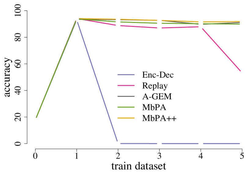
(a) Classification–AGNews

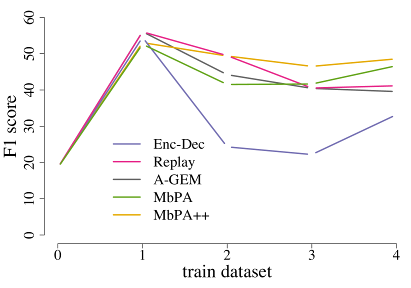
(b) QA–QuAC

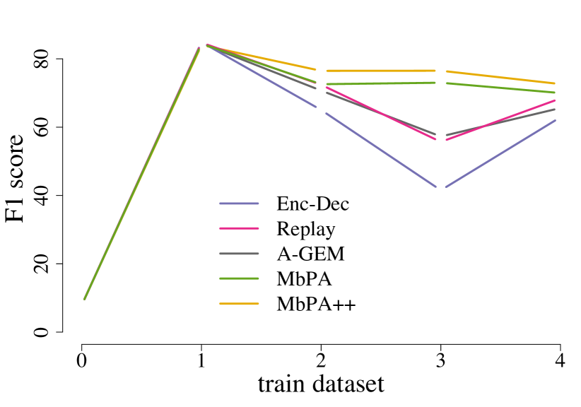
(c) QA–SQuAD

Figure 2: Performance on test examples corresponding to the first dataset seen during training as training progresses.

4.5 Analysis

Memory capacity.

Our results in §4.4 assume that we can store all examples in memory (for all models, including the baselines). We investigate variants of MbPA++ that store only 50% and 10% of training examples. We randomly decide whether to write an example to memory or not (with probability 0.5 or 0.1). We show the results in Table 3. The results demonstrate that while the performance of the model degrades as the number of stored examples decreases, the model is still able to maintain a reasonably high performance even with only 10% memory capacity of the full model.

Number of neighbors.

We investigate the effect of the number of retrieved examples for local adaptation to the performance of the model in Table 3. In both tasks, the model performs better as the number of neighbors increases. Recall that the goal of the local adaptation phase is to shape the output distribution of a test example to peak around relevant classes (or spans) based on retrieved examples from the memory. As a result, it is reasonable for the performance of the model to increase with more neighbors (up to a limit) given a key network that can reliably compute similarities between the test example and stored examples in memory and a good adaptation method.

Table 2: Results with limited memory capacity.

	10%	50%	100%
class.	67.6	70.3	70.6
QA	61.5	61.6	62.0

Table 3: Results for different # of retrieved examples $K$.

	8	16	32	64	128
class.	68.4	69.3	70.6	71.3	71.6
QA	60.2	60.8	62.0	-	-

Computational complexity.

Training MbPA++ takes as much time as training an encoder-decoder model without an episodic memory module since experience replay is performed sparsely (i.e., every 10,000 steps) with only 100 examples. This cost is negligible in practice and we observe no significant difference in terms of wall clock time to the vanilla encoder-decoder baseline. MbPA++ has a higher space complexity for storing seen examples, which could be controlled by limiting the memory capacity.

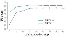
Figure 3: $F_{1}$ scores for MbPA++ and MbPA as the # of local adaptation steps increases.

At inference time, MbPA++ requires a local adaptation phase and is thus slower than methods without local adaptation. This can be seen as a limitation of MbPA++ (and MbPA). One way to speed it up is to parallelize predictions across test examples, since each prediction is independent of others. We set the number of local adaptation steps $L=30$ in our experiments. Figure 3 shows $L\approx 15$ is needed to converge to an optimal performance.

Comparing MBpA++ to other episodic memory models, MBpA has roughly the same time and space complexity as MBpA++. A-GEM, on the other hand, is faster at prediction time (no local adaptation), although at training time it is slower due to extra projection steps and uses more memory since it needs to store two sets of gradients (one from the current batch, and one from samples from the memory). We find that this cost is not negligible when using a large encoder such as BERT.

Analysis of retrieved examples.

In Appendix D, we show (i) examples of retrieved neighbors from our episodic memory model, (iii) examples where local adaptation helps, and (iii) examples that are difficult to retrieve. We observe that the model is able to retrieve examples that are both syntactically and semantically related to a given query derived from a test example, especially when the query is not too short and relevant examples in the memory are phrased in a similar way.

5 Conclusion

We introduced a lifelong language learning setup and presented an episodic memory model that performs sparse experience replay and local adaptation to continuously learn and reuse previously acquired knowledge. Our experiments demonstrate that our proposed method mitigates catastrophic forgetting and outperforms baseline methods on text classification and question answering.

Acknowledgements

We thank Gabor Melis and the three anonymous reviewers for helpful feedback on an earlier draft of this paper.

Appendix A Dataset Order

We use the following dataset orders (chosen randomly) for text classification:

1. Yelp $\rightarrow{}$ AGNews $\rightarrow{}$ DBPedia $\rightarrow{}$ Amazon $\rightarrow{}$ Yahoo.

2. DBPedia $\rightarrow{}$ Yahoo $\rightarrow{}$ AGNews $\rightarrow{}$ Amazon $\rightarrow{}$ Yelp.

3. Yelp $\rightarrow{}$ Yahoo $\rightarrow{}$ Amazon $\rightarrow{}$ DBpedia $\rightarrow{}$ AGNews.

4. AGNews $\rightarrow{}$ Yelp $\rightarrow{}$ Amazon $\rightarrow{}$ Yahoo $\rightarrow{}$ DBpedia.

For question answering, the orders are:

1. QuAC $\rightarrow{}$ TrWeb $\rightarrow{}$ TrWik $\rightarrow$ SQuAD.

2. SQuAD $\rightarrow{}$ TrWik $\rightarrow{}$ QuAC $\rightarrow$ TrWeb.

3. TrWeb $\rightarrow{}$ TrWik $\rightarrow{}$ SQuAD $\rightarrow$ QuAC.

4. TrWik $\rightarrow{}$ QuAC $\rightarrow{}$ TrWeb $\rightarrow$ SQuAD.

Appendix B Full Results

We show per-dataset breakdown of results in Table 1 in Table 4 and Table 5 for text classification and question answering respectively.

Table 4: Per-dataset results on text classification for each ordering and model.

Order	Model	Dataset
		1	2	3	4	5
i	Enc-Dec	1.1	0.0	0.0	4.3	68.7
	A-GEM	42.5	89.8	96.0	56.8	68.2
	Replay	38.2	83.9	95.4	50.3	67.9
	MbPA	42.0	90.4	96.1	52.0	63.9
	MbPA${}^{\text{rand}}_{\text{{+}{+}}}$	35.2	80.4	88.2	45.9	47.2
	MbPA++	45.7	91.6	96.3	54.6	65.6
ii	Enc-Dec	0.0	0.0	3.1	57.9	48.9
	A-GEM	80.1	50.3	91.3	57.3	50.6
	Replay	75.0	53.7	86.0	58.1	50.7
	MbPA	96.0	58.4	89.0	54.4	46.6
	MbPA${}^{\text{rand}}_{\text{{+}{+}}}$	82.0	41.7	81.9	47.1	40.8
	MbPA++	95.8	63.1	92.2	55.7	47.7
iii	Enc-Dec	0.0	0.0	1.3	11.4	93.9
	A-GEM	41.1	55.0	54.6	93.3	93.6
	Replay	23.6	36.8	25.0	94.5	93.8
	MbPA	43.3	60.9	51.6	95.8	92.5
	MbPA${}^{\text{rand}}_{\text{{+}{+}}}$	35.2	33.6	42.1	92.3	82.3
	MbPA++	44.3	62.7	54.4	96.2	93.4
iv	Enc-Dec	0.0	0.0	0.0	14.1	8.1
	A-GEM	90.8	44.9	60.2	65.4	56.9
	Replay	70.4	33.2	39.8	46.1	33.4
	MbPA	89.9	42.9	52.6	62.9	95.1
	MbPA${}^{\text{rand}}_{\text{{+}{+}}}$	78.4	37.7	45.8	42.4	82.9
	MbPA++	91.8	44.9	55.7	65.3	95.8

Table 5: Per-dataset results on question answering for each ordering and model.

Order	Model	Dataset
		1	2	3	4
i	Enc-Dec	34.1	54.2	56.0	85.5
	A-GEM	36.7	51.8	53.4	82.5
	Replay	40.9	56.7	57.2	85.8
	MbPA	45.6	56.1	57.9	83.4
	MbPA${}^{\text{rand}}_{\text{{+}{+}}}$	41.5	56.7	57.2	85.8
	MbPA++	47.2	57.7	58.9	84.3
ii	Enc-Dec	61.9	64.2	29.3	65.0
	A-GEM	64.2	62.5	43.4	63.5
	Replay	67.0	64.1	44.9	65.2
	MbPA	69.9	63.4	43.6	63.3
	MbPA${}^{\text{rand}}_{\text{{+}{+}}}$	67.5	62.5	46.5	63.7
	MbPA++	72.6	63.4	50.5	63.0
iii	Enc-Dec	30.7	31.2	45.6	58.7
	A-GEM	47.6	47.0	57.4	57.4
	Replay	46.6	45.4	53.9	58.3
	MbPA	52.5	54.6	74.5	54.3
	MbPA${}^{\text{rand}}_{\text{{+}{+}}}$	54.1	54.3	71.1	55.9
	MbPA++	56.0	56.8	78.0	54.9
iv	Enc-Dec	55.5	37.1	54.8	85.4
	A-GEM	54.8	38.8	53.4	84.7
	Replay	56.9	41.8	56.4	86.1
	MbPA	58.0	47.2	57.4	83.3
	MbPA${}^{\text{rand}}_{\text{{+}{+}}}$	55.5	43.0	54.6	85.9
	MbPA++	59.0	48.7	58.1	83.6

Appendix C Single Dataset Models

We show results of a single dataset model that is only trained on a particular dataset in Table 6.

Table 6: Performance of a standard encoder-decoder model on each dataset in our experiments. We report accuracy for text classification and $F_{1}$ score for question answering. We also show results from a multitask model for comparisons.

Task	Dataset	Single Model	Multitask
Text Classification	AGNews	93.8	94.0
	Yelp	50.7	50.3
	Amazon	60.1	58.8
	Yahoo	68.6	67.1
	DBPedia	30.5	95.9
	Average	60.7	73.2
Question Answering	QuAC	54.3	56.4
	SQuAD	86.1	85.7
	Trivia Wikipedia	62.3	64.0
	Trivia Web	62.4	64.4
	Average	66.0	67.6

Appendix D Analysis of Retrieved Examples

We analyze retrieved examples to better understand how our model uses its episodic memory.

Examples of retrieved neighbors.

We show examples of retrieved neighbors from memory given a test query in Table 7. We observe that the model is generally able to retrieve relevant examples from the memory. In question answering, nearest neighbors tend to be examples that are both syntactically and semantically related. In text classification, they tend to be articles that discuss the a similar topic.

Examples where local adaptation helps.

In Table 8, we show two test examples where our model answers incorrectly before local adaptation, but correctly after. In the first case, we can see that training examples retrieved from memory are thematically related to the test example. In the second case, since the query is shorter, retrieved training examples tend to be more syntactically related. Although we only show the two nearest neighbors for each query here, our analysis provides an insight on ways our model uses its memory to improve predictions.

Relevant examples that are difficult to retrieve.

In Table 9, we show two relevant training examples (as judged by humans) that are difficult to retrieve by the model (they are not in the 1,000 nearest neighbors) for the query what was the name of bohemond s nephew. The two relevant training examples ask about the nephew of a person, which is relevant for the given query. However, since they are phrased differently to the query, they are far in the embedding space, which is why a nearest neighbor method fails to retrieve these training examples. Our analysis shows that a better embedding and/or retrieval method can potentially improve the performance of our model.

Table 7: Examples of queries and retrieved nearest neighbors for question answering (top) and text classification (truncated, bottom). We also show the corresponding Euclidean distances in parentheses.

Query: in what country is normandy located
(17.48) in what area of france is calais located
(20.37) in what country is st john s located
(22.76) in what country is spoleto located
(23.12) in what part of africa is congo located
(23.83) on what island is palermo located

Query: fears for t n pension after talks unions representing workers at turner newall say they are disappointed after talks with stricken parent firm federal mogul
(37.32) union anger at sa telecoms deal south african unions describe as disgraceful use of public money to buy telecoms shares for former government officials
(47.60) us hurting anti mine campaign anti landmine activists meeting in nairobi say us is setting bad example by not joining worldwide ban
(49.03) woolworths ordered to extend alh takeover deadline independent takeovers panel has headed off woolworths 39 attempts to force resolution in takeover battle for liquor retailer australian leisure and hospitality alh
(50.42) price hike for business broadband small net firms warn they could be hit hard by bt s decision to raise prices for business broadband
(51.08) job fears as deutsche culls chiefs deutsche bank is streamlining management of its investment banking arm raising fears that jobs may be lost in city german bank is reducing number of executives running its investment banking

Table 8: Two examples where local adaptation helps.

Context: david niven ( actor ) - pics , videos , dating , & news david niven male born mar 1 , 1910 james david graham niven , known professionally as david niven , was an english actor and novelist […]
Query: in 1959 , for which film did david niven win his only academy award ?
First two training examples retrieved from memory (2 nearest neighbors):
in which of her films did shirley temple sing animal crackers in my soup ?
in 1968 , which american artist was shot and wounded by valerie solanis , an actress in one of his films ?
Context: dj kool herc developed the style that was the blueprint for hip hop music . herc used the record to focus on a short , heavily percussive part in it : the " break " . […]
Query: what was the break ?
First two training examples retrieved from memory (2 nearest neighbors):
what was the result ?
what was the aftermath ?

Table 9: Relevant examples that are difficult to retrieve from memory.

Query: what was the name of bohemond s nephew
Relevant examples not retrieved (Euclidean distances to the query in parentheses):
(87.88) who was the nephew of leopold
(103.96) who is the nephew of buda king casimer iii the great

References

- Chaudhry et al. (2018) Chaudhry, A., Dokania, P. K., Ajanthan, T., and Torr, P. H. Riemannian walk for incremental learning: Understanding forgetting and intransigence. In Proc. of ECCV, 2018.
- Chaudhry et al. (2019) Chaudhry, A., Ranzato, M., Rohrbach, M., and Elhoseiny, M. Efficient lifelong learning with A-GEM. In Proc. of ICLR, 2019.
- Choi et al. (2018) Choi, E., He, H., Iyyer, M., Yatskar, M., tau Yih, W., Choi, Y., Liang, P., and Zettlemoyer, L. QuAC: Question answering in context. In Proc. of EMNLP, 2018.
- Devlin et al. (2018) Devlin, J., Chang, M.-W., Lee, K., and Toutanova, K. Bert: Pre-training of deep bidirectional transformers for language understanding. In Proc. of NAACL, 2018.
- Howard & Ruder (2018) Howard, J. and Ruder, S. Universal language model fine-tuning for text classification. In Proc. of ACL, 2018.
- Joshi et al. (2017) Joshi, M., Choi, E., Weld, D., and Zettlemoyer, L. Triviaqa: A large scale distantly supervised challenge dataset for reading comprehension. In Proc. of ACL, 2017.
- Kingma & Ba (2015) Kingma, D. P. and Ba, J. L. Adam: a method for stochastic optimization. In Proc. of ICLR, 2015.
- Kirkpatrick et al. (2017) Kirkpatrick, J., Pascanu, R., Rabinowitz, N., Veness, J., Desjardins, G., Rusu, A. A., Milan, K., Quan, J., Ramalho, T., Grabska-Barwinska, A., Hassabis, D., Clopath, C., Kumaran, D., and Hadsell, R. Overcoming catastrophic forgetting in neural networks. Proceedings of the National Academy of Sciences of the United States of America, 114(13):3521–3526, 2017.
- Kitaev & Klein (2018) Kitaev, N. and Klein, D. Constituency parsing with a self-attentive encoder. In Proc. of ACL, 2018.
- Lee et al. (2018) Lee, K., He, L., and Zettlemoyer, L. Higher-order coreference resolution with coarse-to-fine inference. In Proc. of NAACL, 2018.
- Lopez-Paz & Ranzato (2017) Lopez-Paz, D. and Ranzato, M. Gradient episodic memory for continuum learning. In Proc. of NIPS, 2017.
- McCann et al. (2018) McCann, B., Keskar, N. S., Xiong, C., and Socher, R. The natural language decathlon: Multitask learning as question answering. arXiv preprint 1806.08730, 2018.
- McCloskey & Cohen (1989) McCloskey, M. and Cohen, N. J. Catastrophic interference in connectionist networks: The sequential learning problem. In Psychology of Learning and Motivation, volume 24, pp. 109–165. Elsevier, 1989.
- McGaugh (2000) McGaugh, J. L. Memory–a century of consolidation. Science, 287(5451):248–251, 2000.
- Miconi et al. (2018) Miconi, T., Clune, J., and Stanley, K. O. Differentiable plasticity: training plastic neural networks with backpropagation. In Proc. of ICML, 2018.
- Peters et al. (2018) Peters, M. E., Neumann, M., Iyyer, M., Gardner, M., Clark, C., Lee, K., and Zettlemoyer, L. Deep contextualized word representations. In Proc. of NAACL, 2018.
- Rajpurkar et al. (2016) Rajpurkar, P., Zhang, J., Lopyrev, K., and Liang, P. SQuAD: 100,000+ questions for machine comprehension of text. In Proc. of EMNLP, 2016.
- Ramalho & Garnelo (2019) Ramalho, T. and Garnelo, M. Adaptive posterior learning: few-shot learning with a surprise-based memory module. In Proc. of ICLR, 2019.
- Ratcliff (1990) Ratcliff, R. Connectionist models of recognition memory: constraints imposed by learning and forgetting functions. Psychological Review, 97(2):285, 1990.
- Ruder (2017) Ruder, S. An overview of multi-task learning in deep neural networks. arXiv preprint 1706.05098, 2017.
- Schwarz et al. (2018) Schwarz, J., Luketina, J., Czarnecki, W. M., Grabska-Barwinska, A., Teh, Y. W., Pascanu, R., and Hadsell, R. Progress and compress: A scalable framework for continual learning. In Proc. of ICML, 2018.
- Sprechmann et al. (2018) Sprechmann, P., Jayakumar, S. M., Rae, J. W., Pritzel, A., Uria, B., and Vinyals, O. Memory-based parameter adaptation. In Proc. of ICLR, 2018.
- Srivastava et al. (2014) Srivastava, N., Hinton, G., Krizhevsky, A., Sutskever, I., and Salakhutdinov, R. Dropout: A simple way to prevent neural networks from overfitting. Journal of Machine Learning Research, 15:1929–1958, 2014.
- Toneva et al. (2019) Toneva, M., Sordoni, A., des Combes, R. T., Trischler, A., Bengio, Y., and Gordon, G. J. An empirical study of example forgetting during deep neural network learning. In Proc. of ICLR, 2019.
- Vaswani et al. (2017) Vaswani, A., Shazeer, N., Parmar, N., Uszkoreit, J., Jones, L., Gomez, A. N., Kaiser, L., and Polosukhin, I. Attention is all you need. In Proc. of NIPS, 2017.
- Wang et al. (2019) Wang, H., Xiong, W., Yu, M., Guo, X., Chang, S., and Wang, W. Y. Sentence embedding alignment for lifelong relation extraction. In Proc. of NAACL, 2019.
- Yogatama et al. (2019) Yogatama, D., de Masson d’Autume, C., Connor, J., Kocisky, T., Chrzanowski, M., Kong, L., Lazaridou, A., Ling, W., Yu, L., Dyer, C., and Blunsom, P. Learning and evaluating general linguistic intelligence. arXiv preprint 1901.11373, 2019.
- Zenke et al. (2017) Zenke, F., Poole, B., and Ganguli, S. Continual learning through synaptic intelligence. In Proc. of ICML, 2017.
- Zhang et al. (2015) Zhang, X., Zhao, J., and LeCun, Y. Character-level convolutional networks for text classification. In Proc. of NIPS, 2015.