Partial Phase Cohesiveness in Networks of Kuramoto Oscillator Networks

Abstract

Partial, instead of complete, synchronization has been widely observed in various networks including, in particular, brain networks. Motivated by data from human brain functional networks, in this technical note, we analytically show that partial synchronization can be induced by strong regional connections in coupled subnetworks of Kuramoto oscillators. To quantify the required strength of regional connections, we first obtain a critical value for the algebraic connectivity of the corresponding subnetwork using the incremental $2$-norm. We then introduce the concept of the generalized complement graph, and obtain another condition on the weighted nodal degree by using the incremental $\infty$-norm. Under these two conditions, regions of attraction for partial phase cohesiveness are estimated in the forms of the incremental $2$- and $\infty$-norms, respectively. Our result based on the incremental $\infty$-norm is the first known criterion that is applicable to non-complete graphs. Numerical simulations are performed on a two-level network to illustrate our theoretical results; more importantly, we use real anatomical brain network data to show how our results may reveal the interplay between anatomical structure and empirical patterns of synchrony.

I Introduction

Neuronal synchronization across cortical regions of human brain, which has been widely detected through recording and analyzing brain waves, is believed to facilitate communication among neuronal ensembles [1], and only closely correlated oscillating neuronal ensembles can exchange information effectively [2]. In healthy human brain, it is frequently observed that only a part of its cortical regions are synchronized [3], and such a phenomenon is commonly referred to as partial phase cohesiveness or partial synchronization of brain neural networks. In contrast, in pathological brain of a patient such as an epileptic, complete synchronization of neural activities takes place across the entire brain [4]. These observations suggest that healthy brain has powerful regulation mechanisms that are not only able to render synchronization, but also capable of preventing unnecessary synchronization among neuronal ensembles. Partly motivated by these experimental studies, researchers are interested in theoretically studying cluster or partial synchronization [5, 6, 7, 8] and chimera states [9], even though analytical results are much more difficult to obtain, while analytical results for complete synchronization are ample, e.g., [10, 11, 12].

In our research, our ultimate objective is to identify a possible underlying mechanism of partial phase cohesiveness in human brain. Employing the Kuramoto model [13], which has been widely used to describe the dynamics of coupled neural ensembles [14, 15], we analytically study how partial phase cohesiveness can occur in a network of coupled oscillators. In human brain, the organization of cortical neurons exhibits a “network-of-networks” structure in the sense that a cortical region is typically composed of strongly connected ensembles of neurons that interact not only locally but also with ensembles in other regions [16]. As neural ensembles in a cortical region are adjacent in space, it is thus reasonable to assume that oscillators within a brain region are coupled through an all-to-all network, forming local communities at the lower level; at the higher level, the communities are interconnected by a sparse network facilitated through bundles of neural fibers connecting regions of the brain. Motivated by these facts, we consider in this note the networks describing the interaction between Kuramoto oscillators have this two-level structure.

The main contributions of this note are some new sufficient conditions by using Lyapunov functions utilizing the incremental $2$-norm and $\infty$-norm, which ensure partial phase cohesiveness can take place in some subneworks of interest. The incremental $2$-norm was first proposed in [12, 17], in which some conditions for locally exponentially stable synchronization was obtained. Later on, it was also employed in the study of non-complete networks [18, 19]. Inspired by these works, we first employ the incremental $2$-norm and obtain a sufficient condition for the algebraic connectivity $\lambda_{2}(L)$ of the considered subnetwork, and then estimate the region of attraction and the ultimate boundedness of phase cohesiveness. This critical value for $\lambda_{2}(L)$ depends on the natural frequency heterogeneity of the oscillators within the subnetwork and the strength of the connections from its outside to this subnetwork. Since the incremental $2$-norm depends greatly on the scale, the obtained critical value and the estimated region of attraction are both conservative, especially when there are large numbers of oscillators in the considered subnetwork.

On the other hand, the incremental $\infty$-norm is scale independent. It is always utilized to prove the existence of phase-locking manifolds and their local stability. Existing conditions are usually expressed implicitly by a combined measure [20, 21], and the regions of attraction are not estimated [7, 22]. To the authors’ best knowledge, the best result on explicit conditions utilizing the incremental $\infty$-norm is given in [10], which has only studied unweighted complete networks. It is challenging to extend it to the non-complete or even weighted complete networks. To meet the challenges, we introduce a concept of the generalized complement graph in this note, which, in turn, enables us to make use of the incremental $\infty$-norm and obtain an explicit condition. Compared to the results obtained by the incremental $2$-norm: 1) the established sufficient condition is less conservative if the dissimilarity of natural frequencies and the strengths of external connections are noticeable; 2) more importantly, the region of attraction we identified is much larger. After simplifying the network structure, our results on partial phase cohesiveness can reduces to some results on complete phase cohesiveness. The reduced results are sharper than the best known result obtained by using incremental $2$-norm for the case of weighted complete and non-complete networks [19, Theorem 4.6] (especially in terms of the region of attraction), and are identical to the sharpest one found in [10] for the case of unweighted complete networks. The only drawback of our condition is that each oscillator is required to be connected to a minimum number of other oscillators. Finally, we perform some simulations using the anatomical brain network data obtained in [23]; the simulation results show how our theoretical findings may reveal a possible mechanism that gives rise to various patterns of synchrony detected in empirical data of human brain [24]. Our preliminary work was presented in [25], where only the incremental $2$-norm was studied. Moreover, we consider a more general inter-community coupling structure in this note, without requiring that every node in one community is connected to all the nodes in another.

The rest of this note is organized as follows. We introduce the model on the two-level networks and formulate the problem of partial phase cohesiveness in Section II. The first result is obtained by using the incremental $2$-norm in Section III. Section IV introduces the notion of generalized complement graphs and derives the main result utilizing the incremental $\infty$-norm. Some simulations are performed in Section V.

Notations: Let $\mathbb{R}$ and $\mathbb{R}_{\geq 0}$ be the set of real numbers and nonnegative real numbers, respectively. For any positive integer $n$, let $\mathcal{T}_{n}:=\{1,2,\dots,n\}$, and $\mathbf{1}_{n}$ be the all-one vector. Denote the unit circle by $\mathbb{S}^{1}$, and a point on it is called a phase since the point can be used to indicate the phase angle of an oscillator. For any two phases $\gamma_{1},\gamma_{2}\in\mathbb{S}^{1}$, the geodesic distance between them is the minimum of the lengths of the counter-clockwise and clockwise arcs connecting them, which is denoted by $|\gamma_{1}-\gamma_{2}|$. Note that $|\gamma_{1}-\gamma_{2}|\leq\pi$ for any $\gamma_{1},\gamma_{2}$. Let $\mathbb{T}^{n}:=\mathbb{S}^{1}\times\cdots\times\mathbb{S}^{1}$ denote the $n$-torus. For any $x\in\mathbb{R}$, Let $\lfloor x\rfloor$ denote the largest integer that is less than or equal to $x$, and $\lceil x\rceil$ the smallest integer that is greater than or equal to $x$. Let $\|\cdot\|_{p}$ denote the $p$-norm for both vectors and matrices, where $p\geq 1$ can be infinite.

II Problem Setup

We consider a network of $M>1$ communities, each of which consists of $N\geq 1$ fully connected heterogeneous Kuramoto oscillators. The graph of the network, which describes which community is interconnected to which other communities, is in general not a complete graph. The dynamics of the oscillators are described by

$$\dot{\theta}_{i}^{p} =\omega_{i}^{p}+{K^{p}}\sum\nolimits_{n=1}^{N}\sin(\theta^{p}_{n}-\theta_{i}^{p}),$$

$$+ \sum\nolimits_{q=1}^{M}\sum\nolimits_{n=1}^{N}{a^{p,q}_{i,n}}\sin(\theta^{q}_{n}-\theta_{i}^{p}),{p\in\mathcal{T}_{M},i\in\mathcal{T}_{N},}$$ (1)

where $\theta_{i}^{p}\in\mathbb{S}^{1}$ and $\omega_{i}^{p}\geq 0$ represent the phase and natural frequency of the $i$th oscillator in the $p$th community, respectively. Here, the uniform coupling strength of all the edges in the complete graph of the $p$th community is denoted by $K^{p}>0$, which we refer to as the local coupling strengths. The coupling strengths $a^{p,q}_{i,n}$, which we call the inter-community coupling strengths, satisfy $a^{p,q}_{i,n}>0$ if $i\neq n$ and there is a connection between the $i$th oscillator in the $p$th community and the $j$th oscillator in the $q$th community, and $a^{p,q}_{i,n}=0$ otherwise. We define the inter-community coupling matrices by $A^{p,q}:=[a^{p,q}_{i,j}]_{N\times N}\in\mathbb{R}^{N\times N}$, and each satisfies $A^{p,q}=A^{q,p}$.

Remark 1

Our analysis later on applies to the case when each community has a different network topology and even when the numbers of oscillators in the communities are different. However, for the sake of notational simplicity, we assume that each community is connected by a uniformly weighted complete network.

The Kuramoto oscillator network model (1) is used in [14] to study synchronization phenomena of human brain. Along this line of research and motivated by brain research data, we focus on studying the widely observed but still not well understood phenomenon for networks of communities of Kuramoto oscillators, the so called partial phase cohesiveness, in which some but not all of the oscillators have close phases. To facilitate the discussion of some properties of interest for a subset of communities in the network, we use $\mathcal{T}_{r}=\{1,\dots,r\}$, $1\leq r\leq M$, to denote a set of chosen communities with the aim to investigate how phase cohesiveness can occur among these $r$ communities. We then define the following set to capture the situation when the oscillators in the communities in $\mathcal{T}_{r}$ reach phase cohesiveness.

Definition 1

Let $\theta\in\mathbb{T}^{MN}$ be a vector composed of the phases of all $N$ oscillators in all $M$ communities. Then, for a given $\mathcal{T}_{r}$ and $\varphi\in[0,\pi]$, define the partial phase cohesiveness set:

$$\mathcal{S}_{\infty}(\varphi):=\left\{\theta\in\mathbb{T}^{MN}:\max_{i,j\in\mathcal{T}_{N},k,l\in\mathcal{T}_{r}}|\theta_{i}^{k}-\theta_{j}^{l}|\leq\varphi\right\}.$$ (2)

Note that $\varphi$ describes a level of phase cohesiveness since it is the maximum pair-wise phase difference of the oscillators in $\mathcal{T}_{r}$. The smaller $\varphi$ is, the more cohesive the phases are. All the phases in $\mathcal{T}_{r}$ are identical when $\varphi=0$, which is called partial phase synchronization, and this can only happen when all the oscillators have the same natural frequency. In this paper, we allow the natural frequencies to be different, and are only interested in the cases when phase differences in $\mathcal{T}_{r}$ are small enough. We say that partial phase cohesiveness can take place in $\mathcal{T}_{r}$ if the solution ${\theta}:\mathbb{R}_{\geq 0}\to\mathbb{T}^{MN}$ to the system (1) asymptotically converges to this set $\mathcal{S}_{\infty}({\varphi})$ for some $\varphi\in[0,\pi/2)$. We call the particular case when $\mathcal{T}_{r}=\mathcal{T}_{M}$ complete phase cohesiveness, which is also called practical phase synchronization in [11]. In the rest of the paper, we study the partial phase cohesiveness by investigating how a solution $\theta(t)$ can asymptotically converge to the set $\mathcal{S}_{\infty}({\varphi})$ and also by estimating the value of $\varphi$.

Let $\mathcal{G}_{r}=(\mathcal{V}_{r},\mathcal{E}_{r},Z)$ denote the subgraph composed of the nodes in the communities contained in $\mathcal{T}_{r}$ and the edges connecting pairs of them. The weighted adjacency matrix of this subgraph $Z:=[z_{ij}]_{Nr\times Nr}\in\mathbb{R}^{Nr\times Nr}$ is then given by

$$Z:=\left[{\begin{array}[]{*{20}{c}}{{K^{1}}C}&{A^{1,2}}&\cdots&{A^{1,r}}\\ {A^{1,2}}&{{K^{2}}C}&\cdots&{A^{2,r}}\\ \vdots&\vdots&\ddots&\vdots\\ {A^{1,r}}&{A^{2,r}}&\cdots&{{K^{r}}C}\end{array}}\right],$$ (3)

where $C=[c_{ij}]_{N\times N}\in{\mathbb{R}}^{N\times N}$ is the adjacency matrix of a complete graph with $N$ nodes, where $c_{ij}=1$ for $i\neq j$, and $c_{ij}=0$ otherwise (recall that $A^{p,q}$ is symmetric). Let $D:={\rm\;diag}(Z\mathbf{1}_{Nr})$, then the Laplacian matrix of the graph $\mathcal{G}_{r}$ is $L:=D-Z$. Let $\lambda_{2}(L)$ denote the second smallest eigenvalue of $L$, which is always referred to as the algebraic connectivity [26].

Let $\theta^{p}:=[\theta^{p}_{1},\dots,\theta^{p}_{N}]^{\top}$, $\omega^{p}:=$ $[\omega^{p}_{1},\dots,\omega^{p}_{N}]^{\top}$ for all $p\in\mathcal{T}_{M}$. As we are only interested in the behavior of the oscillator in $\mathcal{G}_{r}$, we define $x:=[{\theta^{1}}^{\top},\dots,{\theta^{r}}^{\top}]^{\top}$, and $\varpi:=[{\omega^{1}}^{\top},\dots,{\omega^{r}}^{\top}]^{\top}$. For $i\in\mathbb{N}$, we define $\mu(i):=\lceil i/N\rceil$ and $\rho(i):=i-N\cdot\lfloor i/N\rfloor$. By using these new notations, from (1), the dynamics of the oscillators on $\mathcal{G}_{r}$ can be rewritten as

$${{\dot{x}}_{i}}=\varpi_{i}+ \sum\nolimits_{n=1}^{Nr}{z_{i,n}}\sin({x_{n}}-{x_{i}})$$

$$+\sum\nolimits_{q=r+1}^{M}\sum\nolimits_{n=1}^{N}{a^{\mu(i),q}_{\rho(i),n}}\sin(\theta_{n}^{q}-x_{i}),$$ (4)

where $i\in{\mathcal{T}_{Nr}}$. The first summation term describes the interactions among the oscillators within the subset of communities $\mathcal{T}_{r}$, and the second one represents the interactions from the outside of $\mathcal{T}_{r}$ to the oscillators in $\mathcal{T}_{r}$. In order to study the phase cohesiveness of the oscillators in $\mathcal{G}_{r}$, we then look into the dynamics of pairwise phase differences, given by

$${{\dot{x}}_{i}} -{{\dot{x}}_{j}}={\varpi_{i}}-{\varpi_{j}}$$

$$+\sum\nolimits_{n=1}^{Nr}\left({{z_{i,n}}\sin\left({{x_{n}}-{x_{i}}}\right)}-{{z_{jn}}\sin\left({{x_{n}}-{x_{j}}}\right)}\right)+u_{ij},$$

$$u_{ij}:=\sum\nolimits_{q=r+1}^{M}\sum\nolimits_{n=1}^{N}\Big{(}a^{\mu(i),q}_{\rho(i),n}\sin(\theta_{n}^{q}-x_{i})$$

$$\;\;\;\;\;\;\;\;\;\;\;\;\;\;\;\;\;\;\;\;\;\;\;\;\;\;\;\;\;\;\;\;\;\;\;\;\;\;-{a^{\mu(j),q}_{\rho(j),n}}\sin(\theta_{n}^{q}-x_{j})\Big{)},$$ (5)

where $i,j\in{\mathcal{T}_{Nr}}$. Let $\mathbf{u}_{r}:=[u_{ij}]_{i<j}\in\mathbb{R}^{Nr(Nr-1)/2}$. The incremental dynamics (5) play crucial roles in what follows. In the next two sections, we study partial phase cohesiveness in $\mathcal{G}_{r}$ with the help of (5) using the incremental $2$-norm or $\infty$-norm (which will be introduced subsequently). To analyze phase cohesiveness, the techniques of ultimate boundedness theorem [27, Theorem 4.18] will be employed.

III Incremental $2$-Norm

In this section, we introduce the incremental $2$-norm, and use it as a metric to study partial phase cohesiveness. According to Definition 1, we observe that a partially phase cohesive solution across $\mathcal{T}_{r}$ should satisfy $|x_{i}-x_{j}|\leq\varphi$ for all $i,j\in{\mathcal{T}_{Nr}}$. A quadratic Lyapunov function has been widely used to study phase cohesiveness even when the graph is not complete [17, 12, 11, 19], which is defined by

$$W(x):=\frac{1}{2}\|B_{c}^{\top}x\|_{2}^{2},$$ (6)

where $B_{c}\in\mathbb{R}^{Nr\times(Nr(Nr-1)/2)}$ is the incidence matrix of the complete graph. It is also known as the incremental $2$-norm metric of phase cohesiveness. For a given $\gamma\in[0,\pi)$, define

$${\mathcal{S}_{2}({\gamma})}:=\left\{\theta\in\mathbb{T}^{MN}:\|B_{c}^{\top}x\|_{2}\leq\gamma\right\}.$$ (7)

Note that $\mathcal{S}_{2}({\gamma})\subseteq\mathcal{S}_{\infty}({\gamma})$ for any given $\gamma\in[0,\pi)$. Different from the existing results that apply to complete cohesiveness taking place among all the oscillators in the networks [17, 12, 11, 19], we have studied partial phase cohesiveness in our previous work [25] using the incremental $2$-norm metric. Compared to our previous work, we consider more general inter-community coupling structures as stated in Section II.

Let $\hat{B}_{c}=|B_{c}|$ be the element-wise absolute value of the incidence matrix $B_{c}$. Let $d^{\rm ex}_{i}=\sum\nolimits_{m=r+1}^{M}\sum\nolimits_{n=1}^{N}{a^{\mu(i),m}_{\rho(i),n}}$ for all $i\in\mathcal{T}_{Nr}$, and denote $D^{\rm ex}:=[d^{\rm ex}_{1},\dots,d^{\rm ex}_{Nr}]^{\top}$. Now let us provide our first result on partial phase cohesiveness on incremental $2$-norm. A similar result can be found in [18, Theorem 4.4]. Difference from it, we consider a two-level network, i.e., communities of oscillators, and study the partial phase cohesiveness.

Theorem 1

Assume that the algebraic connectivity of $\mathcal{G}_{r}$ is greater than the critical value specified by

$$\lambda_{2}(L)>\|B_{c}^{\top}\varpi\|_{2}+{\|\hat{B}_{c}^{\top}D^{\rm ex}\|_{2}}.$$ (8)

Then, each of the following equations

$$\lambda_{2}(L)\sin(\gamma_{s})-{\|\hat{B}_{c}^{\top}D^{\rm ex}\|_{2}}=\|B_{c}^{\top}\varpi\|_{2},$$

$$(\pi/2)\lambda_{2}(L){\rm\;sinc}(\gamma_{m})-{\|\hat{B}_{c}^{\top}D^{\rm ex}\|_{2}}=\|B_{c}^{\top}\varpi\|_{2},$$

has a unique solution, $\gamma_{s}\in[0,\pi/2)$ and $\gamma_{m}\in(\pi/2,\pi]$, respectively, where ${\rm\;sinc}(\eta)=\sin(\eta)/\eta$ for any $\eta\in\mathbb{S}^{1}$. Furthermore, the following statements hold:

1. for any $\gamma\in[\gamma_{s},\gamma_{m}]$, $\mathcal{S}_{2}({\gamma})$ is a positively invariant set of the system (1);

2. for any $\gamma\in[\gamma_{s},\gamma_{m})$, the solution to (1) starting from any $\theta(0)\in\mathcal{S}_{2}({\gamma})$ converges to the set $\mathcal{S}_{2}({\gamma_{s}})$.

Proof:

Choose $W(x)$ in (6) as a Lyapunov candidate. Similar to the proof of [19, Theorem 4.6], we take the time derivative of $W(x)$ along the solution to (1) and obtain

$$\dot{W}(x) \leq x^{\top}B_{c}B_{c}^{\top}\varpi$$

$$-{\rm\;sinc}(\gamma)Nrx^{\top}B_{c}{\rm\;diag}(\{z_{ij}\}_{i<j})B_{c}^{\top}x+x^{\top}B_{c}\mathbf{u}_{r}.$$

From [18, Lemma 7], it holds that $x^{\top}B_{c}{\rm\;diag}(\{z_{ij}\}_{i<j})B_{c}^{\top}x$ $\geq\lambda_{2}(L)\|B_{c}^{\top}x\|_{2}^{2}/(Nr)$. From the definition of $\mathbf{u}_{r}$, one can evaluate that $\|\mathbf{u}_{r}\|_{2}\leq\|\hat{B}_{c}^{\top}D^{\rm ex}\|_{2}$. As a consequence, we arrive at

$$\dot{W}(x)\leq x^{\top}B_{c}B_{c}^{\top}\varpi-\lambda_{2}(L) {\rm\;sinc}(\gamma)\|B_{c}^{\top}x\|_{2}^{2}$$

$$+\|B_{c}^{\top}x\|_{2}{\|\hat{B}_{c}^{\top}D^{\rm ex}\|_{2}}.$$

Following similar steps as those in the proof of [19, Theorem 4.6], one can show (i) and (ii) by using the ultimate boundedness theorem [27, Theorem 4.18] under condition (8). ∎

Suppose there is only $1$ oscillator in each community (i.e., $N=1$), and it hold that $\mathcal{T}_{r}=\mathcal{T}_{M}$, $D_{o}=0$, Theorem 1 reduces to the best-known result on the incremental $2$-norm in single level networks [19, Theorem 4.6]. One observes that the established result in Theorem 1 is quite restrictive if the number of oscillators is large because we use the incremental $2$-norm metric. First, the critical value $\lambda_{2}(L)$ is quite conservative since the right side of (8) depends greatly on the number of oscillator in the network. Second, the region of attraction we have identified in Theorem 1(ii) is quite small. To ensure $\|B_{c}^{\top}x(0)\|_{2}<\gamma<\pi$, the initial phases are required to be nearly identical. In the next section, we use incremental-$\infty$ norm, aiming at obtaining less conservative results.

IV Incremental $\infty$-Norm

IV-A Main Results

In this subsection, we take the following function as a Lyapunov candidate for partial phase cohesiveness:

$$V(x)=\|B_{c}^{\top}x\|_{\infty},$$ (9)

which is also referred to as the incremental $\infty$-norm metric. It evaluates the maximum of the pairwise phase differences, and thus does not depend on the number of oscillators. Then, one notices that $\mathcal{S}_{\infty}({\varphi})$ in (2) can be rewritten into

$$\mathcal{S}_{\infty}({\varphi})=\left\{\theta\in\mathbb{T}^{MN}:{V(x)=\|B_{c}^{\top}x\|_{\infty}}\leq\varphi\right\}.$$ (10)

To the best of the authors’ knowledge, the incremental $\infty$-norm has not been used to established explicit conditions for phase cohesiveness analysis in weighted complete or non-complete networks, although some implicit conditions ensuring local stability of phase-locked solutions, such as [20, 21], have been obtained. To obtain explicit conditions by using of the incremental $\infty$-norm, it is always required that the oscillators in a network have the same coupling structures (see [11, Theorem 6.6], [10]). The oscillators in a non-complete network always have distinct coupling structures, which makes the analysis quite challenging. To overcome the challenge, we introduce the notion of the generalized complement graph as follows, which can be viewed as an extension of the complement graph of an unweighted graph.

Definition 2

Consider the weighted undirected graph $\mathcal{G}$ with the weighted adjacency matrix $Z$, and let $K_{m}$ be the maximum coupling strength of its edges. Let $A_{c}$ denote the unweighted adjacency matrix of the complete graph with the same node set as $\mathcal{G}$. We say $\bar{\mathcal{G}}$ is the generalized complement graph of $\mathcal{G}$ if the following two are satisfied: 1) it has the same node set as $\mathcal{G}$; 2) the weighted adjacency matrix is given by $\bar{Z}:=K_{m}A_{c}-Z$.

Let $K_{m}$ be the maximum element in the matrix (3), and $A_{c}$ the unweighted adjacency matrix of the complete graph consisting of the same node set as $\mathcal{G}_{r}$. Then $\bar{Z}=K_{m}A_{c}-Z$ is the weighted adjacency matrix of the generalized complement graph $\bar{\mathcal{G}}_{r}$. In order to enable the analysis using the incremental $\infty$-norm, we then rewrite (II) into the form taking the difference between the complete graph and the generalized complement graph

$$\dot{x}_{i}=\varpi_{i}-K_{m}\sum_{n=1}^{Nr} \sin(x_{i}-x_{n})+\sum_{n=1}^{Nr}\bar{z}_{i,n}\sin(x_{i}-x_{n})$$

$$+\sum_{q=r+1}^{M}\sum_{n=1}^{N}{a^{\mu(i),q}_{\rho(i),n}}\sin(\theta_{n}^{q}-x_{i}),$$

where $i\in{\mathcal{T}_{Nr}}$. Accordingly, the incremental dynamics (5) can be rearranged into

$$\dot{x}_{i} -\dot{x}_{j}=\varpi_{i}-\varpi_{j}-K_{m}\sum_{n=1}^{Nr}\left(\sin(x_{i}-x_{n})-\sin(x_{j}-x_{n})\right)$$

$$+\sum_{n=1}^{Nr}\left(\bar{z}_{in}\sin(x_{i}-x_{n})-\bar{z}_{jn}\sin(x_{j}-x_{n})\right)+u_{ij},$$ (11)

where $i,j\in{\mathcal{T}_{Nr}}$, and $u_{ij}$ is given by (5).

In the incremental $2$-norm analysis, the algebraic connectivity plays an important role since it relates to the matrix induced $2$-norm. When we proceed with the incremental $\infty$-norm analysis, the corresponding ideas in terms of the matrix induced $\infty$-norm are introduced subsequently. Let $\bar{D}_{m}:=\|\bar{Z}\|_{\infty}$, and call it the maximum degree of the generalized complement graph $\bar{\mathcal{G}}_{r}$. Let ${D_{s}^{\rm in}}:=\min_{i=1,\dots,Nr}\sum_{j=1}^{Nr}z_{ij}$, which we call the minimum internal degree of $\mathcal{G}_{r}$. Likewise, let the maximum external degree be $D_{m}^{\rm ex}:=\|D^{\rm ex}\|_{\infty}$. The following proposition provides a relation between the maximum degree of $\bar{\mathcal{G}}_{r}$ and minimum internal degree of $\mathcal{G}_{r}$.

Proposition 1

Given the graph $\mathcal{G}_{r}$, its minimum degree and the maximum degree of the associated generalized complement graph satisfy $\bar{D}_{m}=(Nr-1)K_{m}-D_{s}^{\rm in}$.

Proof:

From $\bar{Z}=K_{m}A_{c}-Z$, the following holds:

$$\bar{z}_{ij}=\left\{\begin{array}[]{ll}0,&i=j\\ K_{m}-z_{ij},&i\neq j.\end{array}\right.$$

By taking the summation with respect to $j$, we have

$$\sum\nolimits_{j=1}^{Nr}\bar{z}_{ij}=(Nr-1)K_{m}-\sum\nolimits_{j=1}^{Nr}z_{ij},$$

where $z_{ii}=0$. From the definition of the $\infty$-norm of the matrix and the fact that all the elements of $\bar{Z}$ and $Z$ are non-negative, it follows that

$$\bar{D}_{m}=\|\bar{Z}\|_{\infty} =\max_{i=1,\dots,Nr}\left((Nr-1)K_{m}-\sum\nolimits_{j=1}^{Nr}z_{ij}\right)$$

$$=(Nr-1)K_{m}-\min_{i=1,\dots,Nr}\sum\nolimits_{j=1}^{Nr}z_{ij}$$

$$=(Nr-1)K_{m}-{D_{s}^{\rm in}}.$$

The proof is complete. ∎

Now we provide our main result in this paper.

Theorem 2

Suppose that the minimum internal degree ${D_{s}^{\rm in}}$ is greater than the critical value specified by

$${D_{s}^{\rm in}}>\frac{\|B_{c}^{\top}\varpi\|_{\infty}+2{D_{m}^{\rm ex}}+(Nr-2)K_{m}}{2}.$$ (12)

Then, there exist two solutions, $\varphi_{s}\in[0,\pi/2)$ and $\varphi_{m}\in(\pi/2,\pi]$, to the equation $\|B_{c}^{\top}\varpi\|_{\infty}+2{D_{m}^{\rm ex}}+2(Nr-1)K_{m}-2{D_{s}^{\rm in}}=NrK_{m}\sin\varphi$, which are given by

$$\varphi_{s}=\arcsin\left(\frac{\|B_{c}^{\top}\varpi\|_{\infty}+2{D_{m}^{\rm ex}}+2(Nr-1)K_{m}-2{D_{s}^{\rm in}}}{NrK_{m}}\right),$$ (13)

$$\varphi_{m}=\pi-\varphi_{s},$$ (14)

respectively. Furthermore, the following statements hold:

1. For any $\varphi\in[\varphi_{s},\varphi_{m}]$, ${\mathcal{S}}_{\infty}(\varphi)$ is a positively invariant set of the system (1);

2. For every initial condition $\theta(0)\in\mathbb{T}^{MN}$ such that $\varphi_{s}<\|B_{c}^{\top}x(0)\|_{\infty}<\varphi_{m}$, the solution $\theta(t)$ to (1) converges to ${\mathcal{S}}_{\infty}(\varphi_{s})$.

Proof:

We first prove (i) by showing that the upper Dini derivative of $V(x(t))$ along the solution to (1),

$$D^{+}V(x(t))=\mathop{\limsup}\limits_{\tau\to 0^{+}}\frac{V({x}(t+\tau))-V({x}(t))}{\tau},$$

satisfies $D^{+}V(x(t))\leq 0$ when $V(x(t))=\varphi$. Define $\mathcal{I}^{\prime}_{M}(t):=\{i:x_{i}(t)=\max_{j\in\mathcal{V}_{r}}x_{j}(t)\}$ and $\mathcal{I}^{\prime}_{S}(t):=\{i:x_{i}(t)=\min_{j\in\mathcal{V}_{r}}x_{j}(t)\}$. Then one can rewrite (9) into

$$V(x(t))=|x_{p}(t)-x_{q}(t)|,\ \forall p\in\mathcal{I}^{\prime}_{M}(t),\forall q\in\mathcal{I}^{\prime}_{S}(t).$$

Let $\mathcal{I}_{M}(t):=\{i:\dot{x}_{i}(t)=\max_{j\in\mathcal{I}^{\prime}_{M}}\dot{x}_{j}(t)\}$ and ${\mathcal{I}_{S}}(t):=\{i:\dot{x}_{i}(t)=\min_{j\in\mathcal{I}^{\prime}_{S}}\dot{x}_{j}(t)\}$. Then the upper Dini Derivative is

$$D^{+}V(x(t))=\dot{x}_{m}(t)-\dot{x}_{s}(t)$$

for all $m\in\mathcal{I}_{M}(t)$ and $s\in\mathcal{I}_{S}(t)$. It follows from (IV-A) that

$$D^{+}V({x}(t))=\dot{x}_{m}-\dot{x}_{s}$$

$$=\varpi_{m}-\varpi_{s}-K_{m}\sum_{n=1}^{Nr}\left(\sin(x_{m}-x_{n})-\sin(x_{s}-x_{n})\right)$$

$$+\sum_{n=1}^{Nr}\left(\bar{z}_{mn}\sin(x_{m}-x_{n})-\bar{z}_{sn}\sin(x_{s}-x_{n})\right)+u_{ms}$$

By using the trigonometric identity $\sin(x)-\sin(y)=2\sin\frac{{x-y}}{2}\cos\frac{x+y}{2}$, we have

$$D {}^{+}V({x}(t))=\varpi_{m}-\varpi_{s}$$

$$-2K_{m}\sum_{n=1}^{Nr}\sin\left(\frac{x_{m}-x_{s}}{2}\right)\cos\left(\frac{x_{m}-x_{n}}{2}-\frac{x_{n}-x_{s}}{2}\right)$$

$$+\sum_{n=1}^{Nr}\left(\bar{z}_{mn}\sin(x_{m}-x_{n})-\bar{z}_{sn}\sin(x_{s}-x_{n})\right)+u_{ms}.$$

Since for any $\varphi\in[0,\pi]$, $V(x(t))=\varphi$ implies that $x_{m}(t)-x_{s}(t)=\varphi$, it follows that

$$-\frac{\varphi}{2}\leq\frac{x_{m}(t)-x_{j}(t)}{2}-\frac{x_{j}(t)-x_{s}(t)}{2}\leq\frac{\varphi}{2}.$$

Consequently, from the double-angle formula $\sin(\varphi)=2\sin(\varphi/2)\cos(\varphi/2)$, it holds that

$$D {}^{+}V({x}(t))\leq\varpi_{m}-\varpi_{s}-NrK_{m}\sin(\varphi)$$

$$+\sum_{n=1}^{Nr}\left(\bar{z}_{mn}\sin(x_{m}-x_{n})-\bar{z}_{sn}\sin(x_{s}-x_{n})\right)+u_{ms}.$$

Recalling the definitions of $\bar{D}_{m}$ and ${D_{m}^{\rm ex}}$, one knows that

$$\left|\sum\nolimits_{n=1}^{Nr}\left(\bar{z}_{mn}\sin(x_{m}-x_{n})-\bar{z}_{sn}\sin(x_{s}-x_{n})\right)\right|\leq 2\bar{D}_{m}$$

and $|u_{ms}|\leq 2{D_{m}^{\rm ex}}$. As a consequence, from $\varpi_{m}-\varpi_{s}\leq\|B_{c}^{\top}\varpi\|_{\infty}$ and Proposition 1, we have

$$D^{+}V({x}(t))\leq \varpi_{m}-\varpi_{s}-NrK_{m}\sin(\varphi)+2\bar{D}_{m}+2{D_{m}^{\rm ex}}$$

$$\leq f(\varphi),$$ (15)

where

$$f(y):=\|B_{c}^{\top}\varpi\|_{\infty} -NrK_{m}\sin(y)$$

$$+2\big{(}(Nr-1)K_{m}-{D_{s}^{\rm in}}\big{)}+2{D_{m}^{\rm ex}}.$$

Now, we aim to find a subinterval in $[0,\pi]$ such that $f(\varphi)\leq 0$ for any $\varphi$ in it. If the condition (12) holds, then $f(\pi/2)<0$ and thus there exists such a subinterval around $\varphi=\pi/2$. Moreover, $\sin(y)$ is an increasing and decreasing function in $[0,\pi/2]$ and $[\pi/2,\pi]$, respectively. Then there always exist two points $y_{1}\in[0,\pi/2),y_{2}\in(\pi/2,\pi]$ such that $f(y_{1})=f(y_{2})=0$. These two points $y_{1}$ and $y_{2}$ are nothing but $\varphi_{s}$ in (13) and $\varphi_{m}$ in (14), respectively. In summary, for any $\varphi\in[\varphi_{s},\varphi_{m}]$, $D^{+}V(x(t))\leq 0$ when $V(x(t))=\varphi$, which implies that ${\mathcal{S}}_{\infty}(\varphi)$ is positively invariant.

Next, we prove (ii). Given $x(0)$, it follows from (15) that for any $t$ there exists $\gamma(t)$ satisfying $\gamma(t)=V(x(t))$ such that

$$D^{+}V(x(t))\leq \|B_{c}^{\top}\varpi\|_{\infty}-NrK_{m}\sin(\gamma(t))$$

$$+2\left((Nr-1)K_{m}-{D_{s}^{\rm in}}\right)+2{D_{m}^{\rm ex}}.$$ (16)

Recalling that the initial condition satisfies that $\varphi_{s}<\|B_{c}^{\top}x(0)\|_{\infty}<\varphi_{m}$, one knows that $\varphi_{s}<\gamma(0)<\varphi_{m}$. Then the right side of (IV-A) is negative, and thus the strict inequality $D^{+}(V(x(0)))<0$ holds. From $t=0$ on, $D^{+}(V(x(0)))<0$ for all $t$ such that $\varphi_{s}<\gamma(t)<\varphi_{m}$, and $D^{+}(V(x(0)))\leq 0$ if $\gamma(t)=\varphi_{s}$. One can then conclude that $\theta(t)$ converges to $\mathcal{S}_{\infty}(\varphi_{s})$. ∎

The following proposition provides a necessary condition for $K_{m}$ such that (12) can be satisfied.

Proposition 2

Suppose that ${D_{s}^{\rm in}}$ satisfies the condition (12), then $K_{m}$ satisfies the following inequality

$$K_{m}>\frac{\|B_{c}^{\top}\varpi\|_{\infty}+2{D_{m}^{\rm ex}}}{Nr}.$$ (17)

Proof:

If the condition (12) is satisfied, we have

$$\|B_{c}^{\top}\varpi\|_{\infty}+2{D_{m}^{\rm ex}}+(Nr-2)K_{m}<2{D_{s}^{\rm in}}.$$

One notices that ${D_{s}^{\rm in}}\leq(Nr-1)K_{m}$ since there are at most $Nr-1$ edges connecting each node, and the coupling strength of each of them is at most $K_{m}$. It then follows that

$$\|B_{c}^{\top}\varpi\|_{\infty}+2{D_{m}^{\rm ex}}+(Nr-2)K_{m}<2(Nr-1)K_{m},$$

which implies $K_{m}>\left({\|B_{c}^{\top}\varpi\|_{\infty}+2{D_{m}^{\rm ex}}}\right)/{Nr}$. ∎

In the study of synchronization or phase cohesiveness, the network is usually required to be connected. The following proposition shows that the condition (12) implies the connectedness of the graph $\mathcal{G}_{r}$ since from the condition (12) the minimum internal degree satisfies ${D_{s}^{\rm in}}>(Nr-2)K_{m}/2$.

Proposition 3

Consider a graph $\mathcal{G}$ consisting of $n$ nodes. Let $K$ be the maximum coupling strength of its edges. Suppose the minimum degree of the nodes satisfies $D_{s}>{(n-2)K}/{2}$, and then the graph $\mathcal{G}$ is connected.

Proof:

We prove this proposition by contradiction. We assume that the graph is not connected, and let $i^{*},j^{*}$ be any two nodes that belongs to two isolated connected components $\mathcal{G}_{i^{*}},\mathcal{G}_{j^{*}}$, respectively. Let the numbers of nodes that are connected to $i^{*},j^{*}$ be $n_{i^{*}}$ and $n_{j^{*}}$, respectively. The degree of $i^{*}$, denoted by $D_{i^{*}}$, satisfies

$$D_{s}\leq D_{i^{*}}\leq n_{i^{*}}K,$$

It follows from the assumption $D_{s}>{(n-2)K}/{2}$ that $n_{i^{*}}>(n-2)/2$. which implies that the number of nodes in $\mathcal{G}_{i^{*}}$ is strictly greater than $n_{i^{*}}+1=n/2$. Likewise, one can show the number of nodes in $\mathcal{G}_{j^{*}}$ is strictly greater than $n_{j^{*}}+1=n/2$. Then the total number of nodes in these two isolated connected components is strictly greater $n_{i^{*}}+n_{j^{*}}+2=n$, which implies the number of node in the graph $\mathcal{G}$ is greater than $n$. This is a contradiction, and thus the network $\mathcal{G}$ is connected. ∎

IV-B Comparisons

We first compare the results in Theorems 1 and 2. It is worth mentioning that the condition in Theorem 2 is less dependent on the number of nodes $Nr$ than that in Theorem 1 in most cases. In sharp contrast to $\|B_{c}^{\top}\varpi\|_{2}$ and ${\|\hat{B}_{c}^{\top}D^{\rm ex}\|_{2}}$ in (8), both $\|B_{c}^{\top}\varpi\|_{\infty}$ and ${D_{m}^{\rm ex}}$ in (12) are independent of $Nr$. Specifically, if we take $\delta_{s},\delta_{m}$ to be the smallest and largest elements in $|B_{c}^{\top}\varpi|$, respectively, it holds that $\delta_{s}\sqrt{Nr(Nr-1)/2}\leq\|B_{c}^{\top}\varpi\|_{2}\leq\delta_{m}\sqrt{Nr(Nr-1)/2}$. A similar inequality holds for ${\|\hat{B}_{c}^{\top}D^{\rm ex}\|_{2}}$. Then, one can observe that $\|B_{c}^{\top}\varpi\|_{2}+{\|\hat{B}_{c}^{\top}D^{\rm ex}\|_{2}}$ in (8) can be much larger than $(Nr-2)K_{m}/2$ in (12) if $Nr$ is large. More importantly, $\mathcal{S}_{\infty}(\varphi)$ is much larger than $\mathcal{S}_{2}(\varphi)$ for the same $\varphi$, which implies that the domain of attraction we estimated in Theorem 2 is much larger than that in Theorem 1. Therefore, the convergence to a partially phase cohesive solution can be guaranteed by Theorem 2 even if the initial phases are not nearly identical.

On the other hand, the condition (8) can be less conservative than (12), but one would require the natural frequencies to be quite homogeneous, and meanwhile the external connections to be very weak in comparison with $K_{m}$. In addition, it can be observed from Proposition 3 that each node in $\mathcal{G}_{r}$ is required to have more than $(Nr-2)/{2}$ neighbors from the condition (12). In this sense, the condition (8) is less conservative since it only requires $\mathcal{G}_{r}$ to be connected.

The following corollary provides a sufficient condition that is independent of the network scale for the partial phase cohesiveness in a dense non-complete subnetwork $\mathcal{G}_{r}$. It is certainly less conservative than its counterpart based on the incremental $2$-norm.

Corollary 1

Suppose each node in $\mathcal{G}_{r}$ is connected by at least $n_{e}$ edges, where $n_{e}>(Nr-2)/2$, and all the edges have the same weight $K$. Assume that

$$K>\frac{\|B_{c}^{\top}\varpi\|_{\infty}+2{D_{m}^{\rm ex}}}{2n_{e}-(Nr-2)},$$ (18)

then the statements (i) and (ii) in Theorem 2 hold.

The proof follows straightforwardly by letting $D_{s}^{\rm in}=n_{e}K$ and $K_{m}=K$. Since $2n_{e}-(Nr-2)\geq 1$, any $K$ satisfying $K>\|B_{c}^{\top}\varpi\|_{\infty}+2{D_{m}^{\rm ex}}$ satisfies the condition (18) for any $Nr$.

Next, we compare our results with the previously-known works in the literature [10, 19]. Since in the existing results, researchers usually deal with one-level networks, and study the complete phase cohesiveness, we assume, in what follows, that there is only one oscillator in each community in our two-level network, and let the set $\mathcal{T}_{r}$ in which we want to synchronize the oscillators be the entire community set $\mathcal{T}_{M}$. Then we obtain the following two corollaries.

Corollary 2

Given an undirected graph $\mathcal{G}$, assume that the following condition is satisfied

$${D_{s}^{\rm in}}>\frac{\|B_{c}^{\top}\varpi\|_{\infty}+(M-2)K_{m}}{2},$$ (19)

then the solutions, $\varphi_{s}\in[0,\pi/2)$ and $\varphi_{m}\in(\pi/2,\pi]$, are respectively given by

$$\varphi_{s}=\arcsin\left(\frac{\|B_{c}^{\top}\varpi\|_{\infty}+2(M-1)K_{m}-2{D_{s}^{\rm in}}}{MK_{m}}\right),$$

$$\varphi_{m}=\pi-\varphi_{s}.$$

Furthermore, the following two statements hold:

1. for any $\varphi\in[\varphi_{s},\varphi_{m}]$, the set ${\mathcal{S}}_{\infty}(\varphi)$ is positively invariant;

2. for every initial condition $x(0)$ such that $\varphi_{s}<|B_{c}^{\top}x(0)\|_{\infty}<\varphi_{m}$, the solution $\theta(t)$ converges to ${\mathcal{S}}_{\infty}(\varphi_{s})$ asymptotically.

This corollary follows from Theorem 2 by letting $N=1$, $r=M$ and ${D_{m}^{\rm ex}}=0$. In this case, $K_{m}=\max_{i,j\in\mathcal{T}_{M}}a_{ij}$ is the maximum coupling strength in $\mathcal{G}$. Compared to the best-known result on the incremental $2$-norm [19, Theorem 4.6], the result established in Corollary 2 is often less conservative. The explanation is similar to what we provide when we compare Theorem 2 with Theorem 1. Assuming the network is complete, we obtain the following corollary.

Corollary 3

Suppose the graph $\mathcal{G}$ is complete, and the coupling strength is $K/M$. Assume that the coupling strength satisfies $K>{\|B_{c}^{\top}\varpi\|_{\infty}}$. Then, $\varphi_{s}$ and $\varphi_{m}$ become

$$\varphi_{s}=\arcsin\left(\frac{\|B_{c}^{\top}\varpi\|_{\infty}}{K}\right), \varphi_{m}=\pi-\varphi_{s}.$$

Furthermore, the statement (i) and (ii) in Corollary 2 hold.

This result is actually identical to the well-known one found in [10, Theorem 4.1], which presents phase cohesiveness on complete graphs with arbitrary distributions of natural frequencies.

V Numerical Examples

In this section, we provide two examples to show the validity of the obtained results (see Example 1), and also to show their applicability to brain networks (see Example 2). We first introduce the order parameter as a measure of phase cohesiveness [13], which is defined by $re^{i\psi}=\frac{1}{n}\sum_{i=1}^{n}e^{i\theta_{j}}$. The value of $r$ ranges from $0$ to $1$. The greater $r$ is, the higher the degree of phase cohesiveness becomes. If $r=1$, the phases are completely synchronized; on the other hand, if $r=0$, the phases are evenly spaced on the unit circle $\mathbb{S}^{1}$.

Example 1

We consider a small two-level network consisting of $6$ communities described in Fig. 1. Each community consists of $5$ oscillators coupled by a complete graph. We assume that the oscillators between every two adjacent communities are interconnected in a way shown in Fig. 1. The inter-community coupling strengths are given beside the edges in Fig. 1. Denote $\omega=[{\omega^{1}}^{\top},\dots,{\omega^{6}}^{\top}]^{\top}$, and let $\omega_{1}=0.5~{}{\rm rad/s}$ and $\omega_{i}=\omega_{1}+0.1(i-1)$ for all $i=2,\dots,30$. Let the local coupling strengths be $K^{2}=K^{3}=2.9$, and $K^{1}=K^{4}=K^{5}=K^{6}=0.01$. One can check that the condition (12) is satisfied for the candidate regions of partial phase cohesiveness in the red rectangular, i.e., $\mathcal{T}_{r}=\{2,3\}$. The evolution of the incremental $\infty$-norm of the oscillators’ phases in $\mathcal{T}_{r}$ is plotted in Fig. 1, from which one can observe that starting from a value less than $\varphi_{m}$, $\|B_{c}^{\top}x(t)\|_{\infty}$ eventually converges to a value less than $\varphi_{s}$. One can then conclude that phase cohesiveness takes place between the communities $2,3$. On the other hand, it can be seen from Fig. 1 that the value of $r$, which measure the level of synchrony, remains small, which means that the other communities in the network are always incoherent. These observations validate our obtained results on partial phase cohesiveness in Theorem 2. Moreover, calculating the algebraic connectivity of the subgraph in the red rectangular, we obtain $\lambda_{2}(L)=5.6$, which is not sufficient to satisfy the condition (8) in Theorem 1. Consistent with what we have claimed earlier, the results in Theorem 2 can be sharper than those in Theorem 1.

Figure 1: (a) The network structure considered in Example 1; (b) the interconnection structure: each oscillator in a community is connected to exact one oscillator in another; (c) the trajectory of $\|B_{c}^{\top}x(t)\|_{\infty}$, where $x=[\theta_{j}^{p}]_{10\times 1},j=\mathcal{T}_{5},p=2,3$; (d) the magnitude $r$ of the order parameter evaluated on other regions ($1,4,5$ and $6$).

Example 2

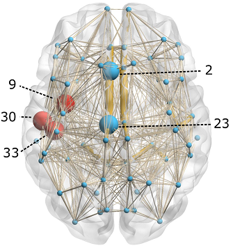
Figure 2: (a) the anatomical brain network visualized by BrainNet Viewer [28], edges only of weights larger than $0.15$ are shown for clarity; (b) the maximum phase difference (absolute value) of the oscillators in $9,30,33$, where $x=[\theta_{j}^{p}]_{30\times 1},j\in\mathcal{T}_{10},p=9,30,33$; (c) the magnitude $r$ of the global order parameter; (d) the magnitude $r$ evaluated on the regions $2$ and $23$.

In this example, we investigate partial phase cohesiveness in human brain with the help of an anatomical network consisting of $66$ cortical regions. The coupling strengths between regions are described by a weighted adjacency matrix $A=[a_{ij}]_{66\times 66}$ whose elements represent axonal fiber densities computed by means of diffusion tensor imaging (DTI). This matrix is the average of the normalized anatomical networks obtained from $17$ subjects [23]. From our earlier analysis, strong regional connections play an essential role in forming partial phase cohesiveness. We identify some candidate regions by selecting the connections of strengths greater than $20$ (visualized by the large size edges in Fig. 2). In particular, we consider two subsets of the brain regions $\{9,30,33\}$ and $\{2,23\}$, (see the red and blue nodes in Fig. 2), and investigate whether phase cohesiveness can occur among them.

We use the model in which each of the $66$ regions consists of $10$ oscillators coupled by a complete graph with the coupling strength $K^{p},p=1,\dots,66$, and any two adjacent regions are connected by $10$ randomly generated edges. The weights of the $10$ edges connecting regions $i$ and $j$ are assigned randomly, and sum up to $a_{ij}$. The natural frequencies of all the oscillators are drawn from a normal distribution with the mean $13\pi{\;\rm rad/s}$ ($6.5{\;\rm Hz}$) and the standard deviation $1.5\pi$. Let the local coupling strengths $K^{p}=8$ for $p=9,30,33$, and $K^{p}=0.1$ for all the other $p$’s. Thus, we have obtained a two-level network from the anatomical brain network. For this two-level network, we obtain some simulation results in Fig. 2, 2 and 2. One can observe from Fig. 2 that the regions $9,30,33$ eventually become phase cohesive, although the whole brain remains quite incoherent (see Fig. 2, where the mean value of $r$ is approximately $0.15$). This observation indicates that strong regional connections can be the cause of partial phase cohesiveness. On the other hand, one observes from Fig. 2 that without strong local coupling strengths phase cohesiveness does not take place between the regions $2$ and $23$ (the blue large nodes in Fig. 2), although they have a strong inter-region connection, $a_{2,23}=52.8023$. This means that local coupling strengths could play an important role in selecting regions to be synchronized.

From our theoretical results and simulations, we believe that there are at least two factors leading to partial brain synchronization. One factor relies on the anatomical properties of the brain network. The second factor depends on local changes of coupling strength. We hypothesize in this note that strong inter-regional coupling is one of the anatomical properties that allow for synchrony among brain regions. Then, selective synchronization of a subset of those strongly connected regions is achieved by increasing the local coupling strengths on the target regions, which can give rise to various synchrony patterns. Other properties of the anatomical brain network such as symmetries studied in [29] and [30], can be a topic of future work.

VI Concluding Remarks

We have studied partial phase cohesiveness, instead of complete synchronization, of Kuramoto oscillators coupled by two-level networks in this note. Sufficient conditions in the forms of algebraic connectivity and nodal degree have been obtained by using the incremental $2$-norm and $\infty$-norm, respectively. The notion of generalized complement graphs that we introduced provides a much better tool than those in the literature to estimate the region of attraction and ultimate level of phase cohesiveness when the network is weighted complete or uncomplete. However, the disadvantage of this method is that the number of edges connecting each node has a noticeable lower bound. The simulations we have performed provides some insight into understanding the partial synchrony observed in human brain. We are interested in investigating other mechanisms that could render partial synchronization.

References

- [1] T. Womelsdorf, J.-M. Schoffelen, R. Oostenveld, W. Singer, R. Desimone, A. K. Engel, and P. Fries, “Modulation of neuronal interactions through neuronal synchronization,” Science, vol. 316, no. 5831, pp. 1609–1612, 2007.
- [2] P. Fries, “A mechanism for cognitive dynamics: Neuronal communication through neuronal coherence,” Trends in Cognitive Sciences, vol. 9, no. 10, pp. 474–480, 2005.
- [3] S. Palva and J. M. Palva, “Discovering oscillatory interaction networks with M/EEG: Challenges and breakthroughs,” Trends in Cognitive Sciences, vol. 16, no. 4, pp. 219–230, 2012.
- [4] R. S. Fisher, W. V. E. Boas et al., “Epileptic seizures and epilepsy: definitions proposed by the International League Against Epilepsy (ILAE) and the International Bureau for Epilepsy (IBE),” Epilepsia, vol. 46, no. 4, pp. 470–472, 2005.
- [5] L. M. Pecora, F. Sorrentino et al., “Cluster synchronization and isolated desynchronization in complex networks with symmetries,” Nature Communications, vol. 5, p. 4079, 2014.
- [6] C. Favaretto, A. Cenedese, and F. Pasqualetti, “Cluster synchronization in networks of Kuramoto oscillators,” in Proc. IFAC World Congr., Toulouse, France, 2017, pp. 2433 – 2438.
- [7] T. Menara, G. Baggio, D. Bassett, and F. Pasqualetti, “Stability conditions for cluster synchronization in networks of heterogeneous Kuramoto oscillators,” IEEE Transactions on Control of Network Systems, doi:10.1109/TCNS.2019.2903914, 2019.
- [8] L. Tiberi, C. Favaretto, M. Innocenti, D. S. Bassett, and F. Pasqualetti, “Synchronization patterns in networks of Kuramoto oscillators: A geometric approach for analysis and control,” in Proc. IEEE Conf. on Decision and Control, Melbourne, Australia, 2017, pp. 7157–7170.
- [9] Y. S. Cho, T. Nishikawa, and A. E. Motter, “Stable chimeras and independently synchronizable clusters,” Physical Review Letters, vol. 119, no. 8, p. 084101, 2017.
- [10] F. Dörfler and F. Bullo, “On the critical coupling for Kuramoto oscillators,” SIAM Journal on Applied Dynamical Systems, vol. 10, no. 3, pp. 1070–1099, 2011.
- [11] ——, “Synchronization in complex networks of phase oscillators: A survey,” Automatica, vol. 50, no. 6, pp. 1539–1564, 2014.
- [12] A. Jadbabaie, N. Motee, and M. Barahona, “On the stability of the Kuramoto model of coupled nonlinear oscillators,” in Proc. IEEE American Control Conf., Boston, MA, USA, 2004, pp. 4296–4301.
- [13] Y. Kuramoto, “Self-entrainment of a population of coupled non-linear oscillators,” in Proc. Int. Symp. Math. Problems Theoret. Phy., Lecture Notes Phys., vol. 39, 1975, pp. 420–422.
- [14] H. Schmidt, G. Petkov et al., “Dynamics on networks: the role of local dynamics and global networks on the emergence of hypersynchronous neural activity,” PLoS Computational Biology, vol. 10, no. 11, p. e1003947, 2014.
- [15] J. Cabral, H. Luckhoo, and et. al., “Exploring mechanisms of spontaneous functional connectivity in meg: How delayed network interactions lead to structured amplitude envelopes of band-pass filtered oscillations,” Neuroimage, vol. 90, pp. 423–435, 2014.
- [16] E. Barreto, B. Hunt et al., “Synchronization in networks of networks: the onset of coherent collective behavior in systems of interacting populations of heterogeneous oscillators,” Physical Review E, vol. 77, no. 3, p. 036107, 2008.
- [17] N. Chopra and M. W. Spong, “On exponential synchronization of Kuramoto oscillators,” IEEE Trans. Autom. Control, vol. 54, no. 2, pp. 353–357, 2009.
- [18] F. Dörfler and F. Bullo, “Synchronization and transient stability in power networks and nonuniform Kuramoto oscillators,” SIAM J. Control Optim., vol. 50, no. 3, pp. 1616–1642, 2012.
- [19] ——, “Exploring synchronization in complex oscillator networks,” in Proc. IEEE Conf. on Decision and Control, Maui, HI, USA, 2012, pp. 7157–7170.
- [20] F. Dörfler, M. Chertkov, and F. Bullo, “Synchronization in complex oscillator networks and smart grids,” Proceedings of the National Academy of Sciences, vol. 110, no. 6, pp. 2005–2010, 2013.
- [21] S. Jafarpour and F. Bullo, “Synchronization of Kuramoto oscillators via cutset projections,” IEEE Trans. Autom. Control, doi: 10.1109/TAC.2018.28767862017.
- [22] T. Menara, G. Baggio, D. S. Bassett, and F. Pasqualetti, “Exact and approximate stability conditions for cluster synchronization of Kuramoto oscillators,” in Proc. American Control Conference, Philadelphia, PA, USA, 2019.
- [23] H. Finger, M. Bönstrup et al., “Modeling of large-scale functional brain networks based on structural connectivity from DTI: Comparison with EEG derived phase coupling networks and evaluation of alternative methods along the modeling path,” PLoS Computational Biology, vol. 12, no. 8, p. e1005025, 2016.
- [24] O. Portoles, J. P. Borst, and M. K. van Vugt, “Characterizing synchrony patterns across cognitive task stages of associative recognition memory,” European Journal of Neuroscience, vol. 48, no. 8, pp. 2759–2769, 2018.
- [25] Y. Qin, Y. Kawano, and M. Cao, “Partial phase cohesiveness in networks of communitinized Kuramoto oscillators,” in Proc. Europ. Control Conf., Limassol, Cyprus, 2018, pp. 2028–2033.
- [26] C. Godsil and G. Royle, Algebraic Graph Theory. Springer, New York, 2001.
- [27] H. K. Khalil, Nonlinear Systems. Prentice-Hall, New Jewsey, 2002.
- [28] M. Xia, J. Wang, and Y. He, “Brainnet Viewer: A network visualization tool for human brain connectomics,” PloS One, vol. 8, no. 7, p. e68910, 2013.
- [29] V. Nicosia, M. Valencia et al., “Remote synchronization reveals network symmetries and functional modules,” Physical Review Letters, vol. 110, no. 17, p. 174102, 2013.
- [30] Y. Qin, Y. Kawano, and M. Cao, “Stability of remote synchronization in star networks of Kuramoto oscillators,” in Proc. IEEE Conf. on Decision and Control, Miami Beach, FL, USA, 2018.