Constraining R-parity-violating couplings in $\displaystyle\tau$-processes at the LHC and
in electroweak precision measurements

Abstract

We find new limits on the $\displaystyle\lambda^{\prime}_{3jk}$ R-parity violating (RPV) couplings of the minimal supersymmetric standard model, using Drell-Yan differential cross sections at the LHC and electroweak precision measurements from LEP and SLC. Specifically, limits on six out of the nine $\displaystyle\lambda^{\prime}_{3jk}$-couplings, with $\displaystyle j=~{}1~{}\text{or}~{}2$, are obtained using Drell-Yan data, with the remaining three (for $\displaystyle j=3$) bounded by precision electroweak data. We also update the limits on all $\displaystyle\lambda^{\prime}_{ijk}$-couplings using electroweak data and find new bounds on $\displaystyle\lambda^{\prime}_{132}$ and $\displaystyle\lambda^{\prime}_{232}$ that are stronger than obtained elsewhere. A table of all current bounds on $\displaystyle\lambda^{\prime}_{ijk}$ is given in an appendix.

I Introduction

With the discovery of the Higgs boson and the completion of the Standard Model (SM) particle spectrum, the search for physics beyond the Standard Model (BSM) is well underway. Among the wide range of possible BSM models, supersymmetry (SUSY) offers a particularly attractive alternative, providing a solution to the hierarchy problem and offering a robust framework for approaching many of the other problems of the SM. But while SUSY may have some very strong theoretical motivations, experiments have yet to find signatures of the most minimal SUSY model in its expected parameter space. This has led physicists to explore less minimal versions of SUSY, including its R-Parity Violating version.

R-parity was originally imposed on the Minimal Supersymmetric Standard Model (MSSM) in an attempt to avoid problems with fast proton decay; as a side effect, it generated an attractive dark matter candidate in the form of the lightest (necessarily stable) SUSY particle (LSP). But the presence of R-parity (or lack thereof) also plays a key role in determining how one should search for the presence of SUSY at colliders like the LHC. In particular, models with unbroken R-parity always pair-produce SUSY particles, and leave missing energy signatures as the SUSY particles decay down to the LSPs, which escape the detector unseen. Most of the key strategies for studying SUSY at colliders involve this particular production path: on-shell pair production, leading to missing energy in the detector. In turn, very strong bounds have been placed on the majority of SUSY particles, constraining their masses to be generally above $\displaystyle 500\,\mathrm{GeV}$ to $\displaystyle 2\,\mathrm{TeV}$ Canepa:2019hph .

In SUSY models with R-parity violation (RPV), the above search strategy generally fails, though other search avenues open up that can help fill the breach. In a previous work (Ref. Bansal:2018dge ), we studied a technique for placing strong constraints on the parameter space from the study of Drell-Yan (DY) processes (both neutral and charged current) at the LHC. In models with RPV, SUSY partners can be exchanged by SM particles at tree level, something that is not possible in R-parity conserving models, leading to sizable interference effects in SM processes. In Ref. Bansal:2018dge , we analyzed the effect of an RPV coupling $\displaystyle\lambda^{\prime}_{ijk}$ (there are 27 such couplings, defined in the next section) on DY processes involving electrons and muons final states. We found that the LHC could already place surprisingly strong constraints in wide regions of the parameter space of squark masses and $\displaystyle\lambda^{\prime}_{ijk}$, for couplings to the first- and second-generation leptons.

In this paper we return to this subject and work to place bounds for the case in which the only available RPV coupling is to $\displaystyle\tau$-leptons using the same techniques. In addition, we revisit precision electroweak constraints on RPV, mostly derived from the LEP and SLC data, to show that the current best fits place stronger constraints on certain $\displaystyle\lambda^{\prime}_{ijk}$ couplings than previously advertised. In all, we will present new bounds on 11 of the 27 $\displaystyle\lambda^{\prime}_{ijk}$ couplings, all of which are stronger than existing bounds found in the literature.

The paper is organized as follows: in section II we will introduce the model and processes that will be studied; we will then present the analysis and results for Drell-Yan processes in section III and electroweak processes in IV; we will devote section V to our conclusions. For completeness, we summarize in the appendix the current bounds on all the 27 $\displaystyle\lambda^{\prime}_{ijk}$ couplings.

II $\displaystyle L$-violating RPV

R-parity is a multiplicative quantum number, defined as

$$R_{P}=(-1)^{3(B-L)+2s}\,,$$ (1)

where $\displaystyle B$ is the baryon number, $\displaystyle L$ the lepton number and $\displaystyle s$ the spin of a specific state. R-parity is usually enforced in the MSSM and allows, as the most general superpotential,

$$\mathcal{W}_{R_{P}}=Y^{u}_{ij}U^{c}_{i}Q_{j}H_{u}-Y^{d}_{ij}D^{c}_{i}Q_{j}H_{d}-Y^{e}_{ij}E^{c}_{i}L_{j}H_{d}+\mu H_{u}H_{d}$$

where $\displaystyle H_{u}$ and $\displaystyle H_{d}$ are two Higgs doublets with hypercharges $\displaystyle\pm 1/2$, respectively. Here, $\displaystyle L$ and $\displaystyle Q$ are the $\displaystyle SU(2)$ doublets, while $\displaystyle E^{c}$, $\displaystyle D^{c}$ and $\displaystyle U^{c}$ are singlets, and $\displaystyle Y^{U}_{ij}$, $\displaystyle Y^{D}_{ij}$ and $\displaystyle Y^{E}_{ij}$ the Yukawa coupling matrices. The above superpotential prevents tree-level processes where $\displaystyle B$ and/or $\displaystyle L$ are violated and has strong phenomenological implications, including the fact that supersymmetric partners should be pair produced in colliders and that the LSP is stable and can become a dark matter candidate. However, in view of the strong experimental bounds on theories with R-parity conservation, one can extend the above superpotential by including R-parity-breaking terms, which soften the present experimental bounds.

In the MSSM, the RPV portion of the trilinear superpotential can be written as,

$$\mathcal{W}_{/R_{P}}=\frac{1}{2}\lambda_{ijk}L_{i}L_{j}E^{c}_{k}+\lambda^{\prime}_{ijk}L_{i}Q_{j}D^{c}_{k}+\frac{1}{2}\lambda^{\prime\prime}_{ijk}U^{c}_{i}D^{c}_{j}D^{c}_{k}.$$

Using the standard notation, we have defined $\displaystyle\lambda_{ijk}$, $\displaystyle\lambda^{\prime}_{ijk}$ and $\displaystyle\lambda^{\prime\prime}_{ijk}$ as new Yukawa couplings, where $\displaystyle i$, $\displaystyle j$ and $\displaystyle k$ are the generation indices; we omit a bilinear term that mixes sleptons and Higgs fields. In order to enforce $\displaystyle B$-conservation, we assume the $\displaystyle\lambda^{\prime\prime}_{ijk}$ are all zero, but $\displaystyle\lambda_{ijk}$ and $\displaystyle\lambda^{\prime}_{ijk}$ remain. Moreover, for the purpose of this work, we will only concentrate on the $\displaystyle\lambda^{\prime}_{ijk}$ interactions. Furthermore, as we did in Ref. Bansal:2018dge , we will only take one element of $\displaystyle\lambda^{\prime}_{ijk}$ at a time to be non-zero, in order to avoid the (possibly) complicated interference effects, and the potentially large contributions to quark or lepton flavor-changing amplitudes.

As we mentioned above, in Ref. Bansal:2018dge , the constraints from Drell-Yan processes on $\displaystyle\lambda^{\prime}_{ijk}$ couplings involving electrons and muons, i.e. $\displaystyle i=1\text{ and }2$, were studied. In this paper, we will concentrate on $\displaystyle\lambda^{\prime}_{ijk}$ couplings involving taus, i.e. $\displaystyle i=3$. In this scenario, the RPV superpotential leads to the following Lagrangian in the $\displaystyle up$-quark mass basis,

$$\displaystyle\mathcal{L} \displaystyle=\lambda^{\prime}_{3jk}\Big{[}\Big{(}(V\bar{d}^{c})_{j}P_{L}\nu_{\tau}-\bar{u}^{c}_{j}P_{L}\tau\Big{)}\tilde{d}_{Rk}^{*}+\Big{(}\bar{d}_{k}P_{L}\nu_{\tau}(V\tilde{d}_{L})_{j}-$$ (2)

$$\displaystyle\bar{d}_{k}P_{L}\tau\tilde{u}_{Lj}\Big{)}+\left(\bar{d}_{k}P_{L}(Vd)_{j}\tilde{\nu}_{\tau L}+\bar{d}_{k}P_{L}u_{j}\tilde{\tau}_{L}\right)\Big{]}+h.c.$$

Here $\displaystyle V$ is the CKM matrix, which we will consider in the (reasonable for our purposes) diagonal approximation.

One of the key points to notice is that the $\displaystyle\lambda^{\prime}_{ijk}$ couplings cause the squarks to couple as scalar leptoquarks; that is, they interact with both quarks and leptons at a single vertex. As such, squarks can be exchanged in the $\displaystyle t$-channel in DY scattering and can appear in loops in $\displaystyle Z$-decay, two processes that we will consider in the following two sections.

In the next two sections, we present our analysis and results for Drell-Yan and electroweak processes, separately.

III Constraints from Drell-Yan processes

The contributions of scalar leptoquarks to DY scattering processes were recently studied in both the neutral current channel Raj:2016aky ; Alves:2018krf and the charged current channel Bansal:2018eha . As with these previous papers, we will refer to the neutral current case as dilepton DY scattering, since the final state is always $\displaystyle\ell^{+}\ell^{-}$ with both leptons of the same flavor (assuming only a single RPV coupling at a time), and the charged current as monolepton DY scattering, since the final state is of the form $\displaystyle\ell\nu_{\ell}$. In Ref Bansal:2018dge , we specialized this analysis to RPV SUSY, studying the $\displaystyle\lambda^{\prime}_{ijk}L_{i}Q_{j}D^{c}_{k}$ superpotential coupling, for $\displaystyle i=1$ (final state electrons) and $\displaystyle i=2$ (final state muons). In both of these final states, excellent analyses of DY data had been completed by both ATLAS and CMS at $\displaystyle\sqrt{s}=13\,\mathrm{TeV}$.

The situation for final state $\displaystyle\tau$-leptons is not as simple at present. DY mono-tau searches have been published by both ATLAS Aaboud:2018vgh and CMS Sirunyan:2018lbg over a wide range of transverse mass. But a similar search for the di-tau process is not available from either of the collaborations. There is a measurement of di-taus from the CMS collaboration Sirunyan:2018qio , but it is limited to small invariant masses ($\displaystyle m_{\tau\tau}<250\,\mathrm{GeV}$) and low integrated luminosity ($\displaystyle 2.3\,\text{fb}^{-1}$). The low invariant mass range studied, and the large statistical errors, will prevent us from placing strong constraints using that data set. Due to these limitations, we will only be able to use the mono-tau DY process to constrain the RPV couplings involving $\displaystyle\tau$-leptons.

The $\displaystyle\lambda^{\prime}_{ijk}$ couplings contribute to the mono-tau process due to the first two terms in Eq. (2) involving $\displaystyle\tilde{d}_{R}^{k}$. After integrating out $\displaystyle\tilde{d}_{R}^{k}$, these terms generate the operator $\displaystyle(\bar{\nu}_{\tau}P_{R}d^{c}_{j})(\bar{u}^{c}_{j}P_{L}\tau)$, which, after fierzing, equals $\displaystyle(1/2)(\bar{d}_{j}\gamma^{\mu}P_{L}u_{j})(\bar{\nu}_{\tau}\gamma_{\mu}P_{L}\tau)$. Thus, this operator directly interferes with the SM process. The Feynman diagrams for this process in the SM and RPV SUSY are shown in Figure 1, with the latter contributing through a $\displaystyle\tilde{d}_{R}^{k}$-mediated $\displaystyle t$-channel process with $\displaystyle d_{j}$ and $\displaystyle u_{j}$ in the initial state. Note that after integrating out $\displaystyle\tilde{d}_{R}^{k}$, the contribution from RPV SUSY only depends on the value of $\displaystyle j$. In other words, for a fixed value of $\displaystyle j$, the constraints on $\displaystyle\lambda^{\prime}_{3jk}$ are the same for all $\displaystyle k$.

Figure 1: Feynman diagrams for mono-tau production in the SM (left) and supersymmetry with RPV (right).

Since quarks in the initial state at LHC have differing parton distribution functions (PDFs), the constraints on $\displaystyle\lambda^{\prime}_{3jk}$ strongly depend on the value of $\displaystyle j$. The constraints are strongest for $\displaystyle j=1$, due to the large PDFs of $\displaystyle u$- and $\displaystyle d$-quarks, followed by somewhat weaker constraints for $\displaystyle j=2$, weaker mostly because of the suppressed PDFs of $\displaystyle c$-quarks. But since the PDF of the top quark can be taken to be zero, $\displaystyle\lambda^{\prime}_{3jk}$ with $\displaystyle j=3$ is not constrained at all. In total, the mono-tau analysis using LHC data can be used to constrain six out of ten $\displaystyle\lambda^{\prime}_{3jk}$ couplings.

We now provide a brief overview of our analysis for Drell-Yan processes, and refer the interested reader to Ref. Bansal:2018dge for a more detailed account. The analysis done here is similar to that of Ref. Bansal:2018dge , with final state electrons and muons replaced by taus. As mentioned above, due to the lack of a di-tau search at the LHC in the right kinematic regime and with sufficient luminosity, we will not be able to use di-tau data to constrain our parameter space. But when the required analysis has been performed by ATLAS and/or CMS, the work done here can be replicated for di-tau processes as well, though a preferable option would be for the collaborations to complete their own interpretation of DY data in terms of bounds on RPV SUSY couplings, following the model here and in Ref. Bansal:2018dge .

As discussed above, the mono-tau DY bounds on $\displaystyle\lambda^{\prime}_{3jk}$ are independent of $\displaystyle k$; that is, the squark mass bounds we obtain are the same for each of the $\displaystyle\tilde{d}_{R}^{k}$ squarks, for $\displaystyle k=1,2,3$. And since we always take $\displaystyle i=3$ (final state as $\displaystyle\tau$-leptons), the only remaining dependence is on $\displaystyle j$. For each value of $\displaystyle j$, we calculate the constraints in the $\displaystyle m_{\tilde{d}_{R}^{k}}~{}\text{versus}~{}\lambda^{\prime}_{3jk}$ plane, by comparing the RPV prediction to the experimental measurements. These measurements are published by both ATLAS Aaboud:2018vgh and CMS Sirunyan:2018lbg collaborations at $\displaystyle\sqrt{s}=13\,\mathrm{TeV}$ with 36 fb^-1 of integrated luminosity. In this work, we compare with the ATLAS data as they are readily available at www.hepdata.net. The signal events are obtained by simultaneously calculating the SM plus RPV contribution to the transverse mass $\displaystyle(m_{T})$ spectrum for $\displaystyle pp\to\tau\nu_{\tau}$ processes. These calculations are done analytically at the leading order, using the MSTW 2008 NNLO PDFs Martin:2009iq . The resulting spectrum is then rescaled bin-by-bin to account for the higher-order corrections and lepton reconstruction efficiency, so that our SM (“background”) spectrum matches the irreducible background data from ATLAS. Finally, the net signal plus background is obtained by adding the reducible background to the generated event distribution.

To quantify the effect of our signal, and to estimate the limits on the RPV parameters, we use a conservative version of a $\displaystyle\Delta\chi^{2}$ test. Specifically, 95% C.L. limits are obtained when $\displaystyle\Delta\chi^{2}\equiv\chi^{2}_{\text{model}}-\chi^{2}_{\text{SM}}=5.99$. The systematic errors used in this test are taken, bin by bin, from the ATLAS searches Aaboud:2018vgh , which range from about 15% at low transverse masses ($\displaystyle\sim 200$ GeV) to over 50% at high transverse masses. Finally, we quote our limits on the model by fitting a straight line in the $\displaystyle(m_{\tilde{d}_{R}^{k}},\lambda^{\prime}_{3jk})$-plane to the 95% C.L. contour in the region where $\displaystyle m_{\tilde{d}_{R}^{k}}\geq 1\,\mathrm{TeV}$. Below $\displaystyle 1\,\mathrm{TeV}$ squark masses, the constraints are far less linear, and the squarks themselves are often better constrained by direct production limits. Thus, the limits we quote only hold for $\displaystyle m_{\tilde{d}_{R}^{k}}>1\,\mathrm{TeV}$. The accuracy of our linear fit can be seen in Figure 2, where the 95% C.L. contour (solid line) and a linear fit (dashed line) to this contour are shown for $\displaystyle\lambda^{\prime}_{31k}$.

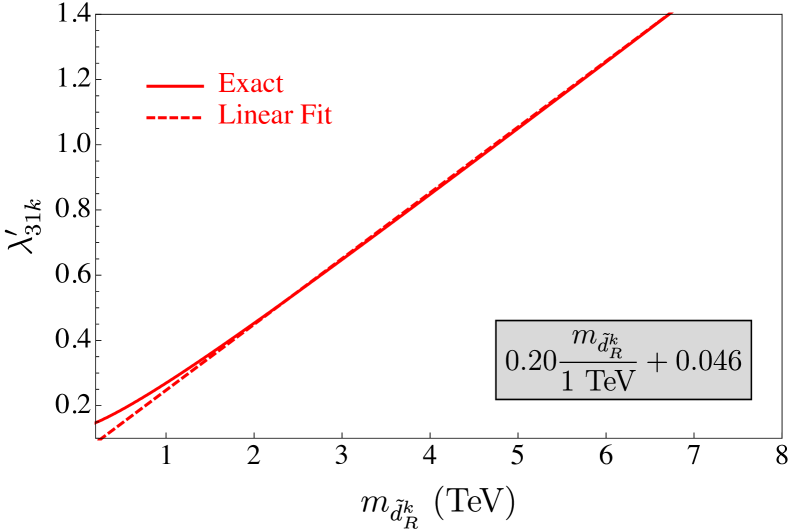
Figure 2: The 95% C.L. upper bound (solid line) on $\displaystyle\lambda^{\prime}_{31k}$ using monolepton data. A linear fit (dashed line) to this bound and the corresponding equation are also shown.

Our resulting constraints from monolepton DY processes are summarized in the second column of Table 1. The first column indicates the existing bound in the literature, collected and updated in Refs. Barger:1989rk ; ledroit:in2p3 ; Allanach:1999ic ; Barbier:2004ez ; Chemtob:2004xr ; Dercks:2017lfq . These bounds are derived from: $\displaystyle R_{\tau\pi}=\Gamma(\tau\to\pi\nu_{\tau})/\Gamma(\mu\to\pi\nu_{\mu})$ for $\displaystyle\lambda^{\prime}_{31k}$; $\displaystyle R_{D_{s}}=\Gamma(D_{s}\to\tau\nu_{\tau})/\Gamma(D_{s}\to\mu\nu_{\mu})$ for $\displaystyle\lambda^{\prime}_{32k}$; and $\displaystyle R_{\tau}=\Gamma(Z\to\text{had})/\Gamma(Z\to\tau\bar{\tau})$ for $\displaystyle\lambda^{\prime}_{33k}$. The constraints on $\displaystyle\lambda^{\prime}_{33k}$ are discussed in more detail below.

$\displaystyle ijk$	Literature	Monolepton	Electroweak	Projected
$\displaystyle 31k$	$\displaystyle 1.1\frac{m_{\tilde{d}_{R}^{k}}}{1\,\mathrm{TeV}}$	$\displaystyle 0.20\frac{m_{\tilde{d}_{R}^{k}}}{1\,\mathrm{TeV}}+0.046$	$\displaystyle 1.5\frac{m_{\tilde{f}}}{1\,\mathrm{TeV}}+0.41$	$\displaystyle 0.14\frac{m_{\tilde{d}_{R}^{k}}}{1\,\mathrm{TeV}}+0.046$
$\displaystyle 32k$	$\displaystyle 5.2\frac{m_{\tilde{d}_{R}^{k}}}{1\,\mathrm{TeV}}$	$\displaystyle 1.5\frac{m_{\tilde{d}_{R}^{k}}}{1\,\mathrm{TeV}}+0.66$	$\displaystyle 1.5\frac{m_{\tilde{f}}}{1\,\mathrm{TeV}}+0.41$	$\displaystyle 0.75\frac{m_{\tilde{d}_{R}^{k}}}{1\,\mathrm{TeV}}+0.69$
$\displaystyle 33k$	$\displaystyle 1.24^{\dagger}$	$\displaystyle-$	$\displaystyle 0.54\frac{m_{\tilde{f}}}{1\,\mathrm{TeV}}+0.38$	$\displaystyle-$

Table 1: Upper bounds on $\displaystyle\lambda^{\prime}_{3jk}\ (k=1,2,3)$ from the literature and derived in this study. The strongest current constraint on a particular coupling (for $\displaystyle m_{\tilde{f}}>1\,\mathrm{TeV}$) is shown in a box. Projected bounds are obtained using a mono-tau analysis assuming $\displaystyle 3\,\mbox{ab}^{-1}\!$ of data.  ^†See text for an explanation of this bound which holds for sfermion masses of 1 TeV.

One must note that the current ATLAS mono-tau data show a small excess over the SM predictions for most of the $\displaystyle m_{T}$-bins. On the other hand, the RPV monolepton operator interferes destructively with the SM, pulling down the expected cross section. Thus the resulting constraints on $\displaystyle\lambda^{\prime}_{3jk}$ are much stronger than one would expect just by comparing to the SM distribution. This same excess of events in the data also results in a constraint on $\displaystyle\lambda^{\prime}_{32k}$ that is surprisingly strong despite being suppressed by the $\displaystyle c$-quark PDF. Thus one should keep in mind that if the mono-tau data were to become more closely aligned with the SM prediction, the bounds would weaken. Similar observations were also made for mono-muons in Ref. Bansal:2018dge .

Unsurprisingly, the limits we obtain are very sensitive to current experimental uncertainties in the DY spectrum, and so these limits may strengthen or weaken with higher integrated luminosity, at least at first. But we can also make a simple projection of the expected limits on $\displaystyle\{m_{\tilde{q}},\lambda^{\prime}_{ijk}\}$ at the High Luminosity LHC with $\displaystyle 3\,\mbox{ab}^{-1}\!$ of integrated luminosity and $\displaystyle\sqrt{s}=13\,\mathrm{TeV}$, assuming the data matches the SM predictions. In this analysis, we again use the transverse mass dependent systematic error as seen across bins in the current ATLAS data and neglect all sources of reducible background. The last column of Table 1 indicates these expected limits from a $\displaystyle 3\,\mbox{ab}^{-1}\!$ high luminosity LHC.

As expected, the constraints obtained from the LHC monolepton analysis are strongest when the quarks involved are first generation, and weaken significantly when one requires second generation quarks in the initial state (by roughly a factor of 10 in going from $\displaystyle\lambda^{\prime}_{31k}$ to $\displaystyle\lambda^{\prime}_{32k}$). In such a case, the dilepton bound would be expected to outdo the monolepton bound, which is another reason why the absence of an experimental DY dilepton analysis hampers the setting of the strongest possible bounds right now. For $\displaystyle\lambda^{\prime}_{33k}$, monolepton searches at the LHC are completely insensitive and another route must be sought in order to obtain bounds on this coupling; we discuss this case in the next section.

IV Electroweak Constraints

LHC bounds on the $\displaystyle\lambda^{\prime}_{33k}$ couplings are non-existent currently, and will be weak, at best, in the future (using dilepton data, once available). Luckily, there is a well-known auxiliary bound that can be placed on all of the RPV couplings coming from precision electroweak observables. In particular, the RPV couplings can affect electroweak observables at one loop by modifying the coupling strength of $\displaystyle Z$ to fermions. Since these observables have been measured very precisely by both LEP and SLC at, and above, the $\displaystyle Z$-pole, the $\displaystyle\lambda^{\prime}_{ijk}$ couplings can be constrained by quantifying these modifications. This requires the calculation of RPV-induced $\displaystyle Z\to f\bar{f}$ one-loop diagrams, shown in Figure 3, where $\displaystyle f$ is any of $\displaystyle\ell_{i}$, $\displaystyle\nu_{i}$, $\displaystyle u_{j}$, $\displaystyle d_{j}$ and $\displaystyle d_{k}$ for a non-zero $\displaystyle\lambda^{\prime}_{ijk}$. Each final state $\displaystyle f$ can have multiple different fermions and sfermions in the loop; for example, a non-zero $\displaystyle\lambda^{\prime}_{332}$ can lead to $\displaystyle Z\to\tau\bar{\tau}$ with $\displaystyle t_{L}$-quark and $\displaystyle\tilde{s}_{R}$ as well as $\displaystyle s_{R}$-quark and $\displaystyle\tilde{t}_{L}$ in the loop. By calculating all the possible one-loop diagrams for a single non-zero $\displaystyle\lambda^{\prime}_{ijk}$, the RPV parameter space is constrained.

(a)

(b)

(c)

(d)

Figure 3: Feynman diagrams for $\displaystyle Z\to f\bar{f}$ via RPV couplings. The dashed lines represent the exchange of the scalars $\displaystyle S$ and/or $\displaystyle\tilde{S}$ defined in the text.

One may expect that the effect of one-loop diagrams with $\displaystyle\mathcal{O}(\,\mathrm{TeV})$ sfermion masses would be negligible at the $\displaystyle Z$-pole. But it has long been known (e.g., Mizukoshi:1994zy ; ColuccioLeskow:2016dox ; Bansal:2018nwp ) that the contribution of these diagrams with $\displaystyle t$-quarks in the loop can be fairly large. This is the result of helicity flips on the $\displaystyle t$-quark lines. Since the $\displaystyle\lambda^{\prime}_{ijk}$ couplings can contribute a $\displaystyle t$-quark for $\displaystyle j=3$, we expect relatively strong electroweak constraints on $\displaystyle\lambda^{\prime}_{i3k}$. In this section, we will analyze the contributions of RPV to precision electroweak observables in order to constrain the set of couplings $\displaystyle\lambda^{\prime}_{i3k}$. We are hardly the first to do this analysis; previous analyses were performed by Refs. Godbole:1992fb ; Bhattacharyya:1995pr ; Yang:1999ms ; Lebedev:1999vc ; Lebedev:1999ze ; ledroit:in2p3 . Our analysis uses updated electroweak parameters (mostly updated SM predictions for the precision electroweak observables) that have the effect of strengthening the bounds somewhat. But we will also be using an alternative observable, defined below, that allows for an improvement on the electroweak constraints on $\displaystyle\lambda^{\prime}_{33k}$ of roughly 25% for sfermion masses of $\displaystyle 1\,\mathrm{TeV}$. As a cross check, we also performed our fits using the observables, data and SM fits of previous authors, and successfully reproduced the previously obtained bounds.

Before specializing to the problem at hand, we first stop to consider a somewhat more general calculation. Consider a toy model with two scalars, $\displaystyle S$ and $\displaystyle\tilde{S}$, which interact with the fermions of the SM through the Lagrangian:

$$\displaystyle\mathcal{L}=\sum_{X=L,R}\left\{\lambda_{X}S\,\overline{f^{\prime c}}f_{X}+\tilde{\lambda}_{X}\tilde{S}\bar{f^{\prime}}f_{X}+h.c.\right\}$$ (3)

Here $\displaystyle f_{L,R}$ and $\displaystyle f^{\prime}_{L,R}$ are chiral SM states with their usual gauge quantum numbers, while the quantum numbers of $\displaystyle S$ and $\displaystyle\tilde{S}$ are chosen such that the terms in the Lagrangian are gauge invariant. These scalars can then modify the $\displaystyle Z\to\bar{f}f$ amplitude through the Feynman diagrams shown in Fig. 3, with $\displaystyle f^{\prime}$ being the loop fermion. Since there is a discontinuity in the amplitude of the first diagram (Fig. 3(a)) at $\displaystyle m_{f^{\prime}}=m_{Z}/2$, the contributions from these diagrams can be divided into two cases: for $\displaystyle m_{f^{\prime}}\simeq 0$ and $\displaystyle m_{f^{\prime}}>m_{Z}/2$. All the fermions of the SM fall into the first category except for the $\displaystyle t$-quark, which clearly belongs to the second case. Meanwhile, we assume the common mass of all scalars, denoted by $\displaystyle M$, to be much greater than $\displaystyle m_{Z}$ and thus there is no discontinuity in the second diagram (Fig. 3(b)).

We can absorb the contributions from the one-loop diagrams into a redefinition of the the $\displaystyle Z\bar{f}f$ couplings, via:

$$\mathcal{L}_{Z}=\frac{g_{2}}{c_{w}}\,\sum_{X=L,R}\left(g_{X}^{f}+\Delta g_{X}^{f}\right)Z_{\mu}\,\bar{f}_{X}\gamma^{\mu}f_{X}$$ (4)

where $\displaystyle g_{L}^{f}=T_{3}^{f}-Q^{f}s_{w}^{2}$, $\displaystyle g_{R}^{f}=-Q^{f}s_{w}^{2}$, and $\displaystyle T_{3}^{f}$ is the weak $\displaystyle T_{3}$ of the left-handed fermion $\displaystyle f_{L}$. The leading order corrections to the $\displaystyle Z\bar{f}f$ couplings due to $\displaystyle S$, taken from Appendix B of Ref. Bansal:2018nwp , can be written as:

Case I: $\displaystyle m_{f^{\prime}}\sim 0$:

$$\displaystyle\Delta g^{f}_{L/R}=\frac{|\lambda_{L/R}|^{2}m_{Z}^{2}N_{c}^{f^{\prime}}}{288\pi^{2}M^{2}N_{c}^{f}}\times$$

$$\displaystyle~{}~{}~{}~{}~{}~{}~{}\left\{g^{f}_{L/R}-g^{f^{\prime}}_{L/R}\left(12\log\frac{M}{m_{Z}}+1+\bm{i}6\pi\right)\right\}$$ (5)

Case II: $\displaystyle m_{f^{\prime}}>m_{Z}/2$:

$$\displaystyle\Delta g^{f}_{L/R}=\pm\frac{|\lambda_{L/R}|^{2}m_{f^{\prime}}^{2}T_{3}^{f^{\prime}}N_{c}^{f^{\prime}}}{16\pi^{2}M^{2}N_{c}^{f}}\left(2\log\frac{M}{m_{f^{\prime}}}-1\right)+$$

$$\displaystyle\frac{|\lambda_{L/R}|^{2}m_{Z}^{2}N_{c}^{f^{\prime}}}{288\pi^{2}M^{2}N_{c}^{f}}\left\{g^{f}_{L/R}-g^{f^{\prime}}_{L/R}\left(12\log\frac{M}{m_{f^{\prime}}}-9\right)\pm 3T_{3}^{f^{\prime}}\right\},$$ (6)

where $\displaystyle M$ is the mass of $\displaystyle S$, and $\displaystyle N_{c}^{f,f^{\prime}}$ is the color factor of the final fermion state, $\displaystyle f$, or of the internal loop fermion, $\displaystyle f^{\prime}$ (i.e., 3 for a color triplet, 1 for a singlet). The imaginary piece that arises in Case I is due to the loop fermions going on shell, but does not contribute to $\displaystyle Z$-pole observables. Also note that the $\displaystyle\pm 3T_{3}^{f^{\prime}}$ term at the end of Eq. (IV) corrects a typographical error in Ref. Bansal:2018nwp .

Similarily, on computing the amplitudes involving $\displaystyle\tilde{S}$, we find the dominant parts of the corrections to $\displaystyle Z\bar{f}f$ couplings for the two cases to be:

Case I: $\displaystyle m_{f^{\prime}}\sim 0$:

$$\displaystyle\Delta g^{f}_{L/R}=\frac{|\tilde{\lambda}_{L/R}|^{2}m_{Z}^{2}N_{c}^{f^{\prime}}}{288\pi^{2}M^{2}N_{c}^{f}}\times$$

$$\displaystyle~{}~{}~{}~{}~{}~{}~{}\left\{g^{f}_{L/R}+g^{f^{\prime}}_{R/L}\left(12\log\frac{M}{m_{Z}}+1+\bm{i}6\pi\right)\right\}$$ (7)

Case II: $\displaystyle m_{f^{\prime}}>m_{Z}/2$:

$$\displaystyle\Delta g^{f}_{L/R}=\pm\frac{|\tilde{\lambda}_{L/R}|^{2}m_{f^{\prime}}^{2}T_{3}^{f^{\prime}}N_{c}^{f^{\prime}}}{16\pi^{2}M^{2}N_{c}^{f}}\left(2\log\frac{M}{m_{f^{\prime}}}-1\right)+$$

$$\displaystyle\frac{|\tilde{\lambda}_{L/R}|^{2}m_{Z}^{2}N_{c}^{f^{\prime}}}{288\pi^{2}M^{2}N_{c}^{f}}\left\{g^{f}_{L/R}+g^{f^{\prime}}_{R/L}\left(12\log\frac{M}{m_{f^{\prime}}}-9\right)\pm 3T_{3}^{f^{\prime}}\right\},$$ (8)

where $\displaystyle M$ is now the mass of $\displaystyle\tilde{S}$.

Note that these relations are only valid up to leading order in $\displaystyle m_{Z}/M$ and $\displaystyle m_{f^{\prime}}/M$. Nonetheless, in Eqs. (IV) and (IV), the terms proportional to $\displaystyle m_{f^{\prime}}^{2}$ will be much larger than the ones proportional to $\displaystyle m_{Z}^{2}$ when the internal fermion, $\displaystyle f^{\prime}$, is taken to be the top quark. Thus it will be these terms, proportional to $\displaystyle m^{2}_{f^{\prime}}=m^{2}_{t}$, that are particularly constrained by electroweak precision measurements.

The interactions in the RPV Lagrangian in Eq. (2) mimic those of our toy model in Eq. (3). Thus, Eqs. (IV)-(IV) can also be used to compute the RPV-induced corrections to the $\displaystyle Z\bar{f}f$ couplings. To calculate the modification in the $\displaystyle Z\bar{f}f$ coupling for a fixed final state $\displaystyle f$, the contributions from all the possible virtual states that can couple to $\displaystyle f$ should be combined. For instance, a non-zero $\displaystyle\lambda^{\prime}_{332}$ can modify the $\displaystyle Z\bar{\tau}\tau$ coupling, in addition to the $\displaystyle Z\bar{\nu}_{\tau}\nu_{\tau}$, $\displaystyle Z\bar{b}b$ and $\displaystyle Z\bar{s}s$ couplings. For the final state $\displaystyle\tau$, there can be two combinations of fermions and sfermions in the loop, i.e., $\displaystyle t_{L}$-quark and $\displaystyle\tilde{s}_{R}$, and $\displaystyle s_{R}$-quark and $\displaystyle\tilde{t}_{L}$. The contributions from these two virtual states can be calculated using Eqs. (IV) and (IV) to obtain the correction to the $\displaystyle Z-\tau_{L}$ interaction:

$$\displaystyle\Delta g_{L}^{\tau}(\mbox{from }\lambda^{\prime}_{332})=$$

$$\displaystyle~{}~{}~{}\frac{3|\lambda^{\prime}_{332}|^{2}m_{t}^{2}}{32\pi^{2}m_{\tilde{s}_{R}}^{2}}\left(2\log\frac{m_{\tilde{s}_{R}}}{m_{t}}-1\right)+\frac{|\lambda^{\prime}_{332}|^{2}m_{Z}^{2}}{96\pi^{2}m_{\tilde{t}_{L}}^{2}}\times$$

$$\displaystyle\left\{\left(-\frac{1}{2}+s_{w}^{2}\right)+\left(\frac{1}{3}s_{w}^{2}\right)\left(12\log\frac{m_{\tilde{t}_{L}}}{m_{Z}}+1+\bm{i}6\pi\right)\right\}$$ (9)

In the above equation, we have ignored a negligible contribution proportional to $\displaystyle m_{Z}^{2}/m_{\tilde{s}_{R}}^{2}$, arising from the second term of Eq. (IV). A similar analysis can be done for any non-zero $\displaystyle\lambda^{\prime}_{ijk}$ in any $\displaystyle Z\to f\bar{f}$ channel.

The RPV parameter space is constrained by using $\displaystyle\Delta g^{f}$ to predict the $\displaystyle Z$-pole observables and comparing them with their experimental measurements. The electroweak observables used in this work are shown in Table 2, where: $\displaystyle\Gamma(\text{inv})$ is the invisible decay width of the $\displaystyle Z$, $\displaystyle R_{\ell}\equiv\Gamma(\text{had})/\Gamma(\ell\bar{\ell})$, $\displaystyle R_{q}\equiv\Gamma(q\bar{q})/\Gamma(\text{had})$, and $\displaystyle A_{f}\equiv(2g_{A}^{f}g_{V}^{f})/((g_{A}^{f})^{2}+(g_{V}^{f})^{2})$. In these expressions, $\displaystyle\Gamma(\text{had})$ is the partial width of $\displaystyle Z$ into hadrons, and $\displaystyle g_{V}^{f}$ and $\displaystyle g_{A}^{f}$ are the effective vector and axial couplings of $\displaystyle Z\to f\bar{f}$.

Observable	Experimental	Standard Model	Pull
$\displaystyle\Gamma(\text{inv})~{}[\text{MeV}]$	$\displaystyle 499.0\pm 1.5$	$\displaystyle 501.66\pm 0.05$	$\displaystyle-1.8$
$\displaystyle R_{e}$	$\displaystyle 20.804\pm 0.050$	$\displaystyle 20.734\pm 0.010$	$\displaystyle 1.4$
$\displaystyle R_{\mu}$	$\displaystyle 20.785\pm 0.033$	$\displaystyle 20.734\pm 0.010$	$\displaystyle 1.6$
$\displaystyle R_{\tau}$	$\displaystyle 20.764\pm 0.045$	$\displaystyle 20.779\pm 0.010$	$\displaystyle-0.3$
$\displaystyle R_{b}$	$\displaystyle 0.21629\pm 0.00066$	$\displaystyle 0.21579\pm 0.00003$	$\displaystyle 0.8$
$\displaystyle R_{c}$	$\displaystyle 0.1721\pm 0.0030$	$\displaystyle 0.17221\pm 0.00003$	$\displaystyle 0.0$
$\displaystyle A_{e}$	$\displaystyle 0.15138\pm 0.00216$	$\displaystyle 0.1470\pm 0.0004$	$\displaystyle 2.0$
$\displaystyle A_{\mu}$	$\displaystyle 0.142\pm 0.015$	$\displaystyle 0.1470\pm 0.0004$	$\displaystyle-0.7$
$\displaystyle A_{\tau}$	$\displaystyle 0.1439\pm 0.0043$	$\displaystyle 0.1470\pm 0.0004$	$\displaystyle-0.7$
$\displaystyle A_{b}$	$\displaystyle 0.923\pm 0.020$	$\displaystyle 0.9347$	$\displaystyle-0.6$
$\displaystyle A_{c}$	$\displaystyle 0.670\pm 0.027$	$\displaystyle 0.6678\pm 0.0002$	$\displaystyle 0.1$
$\displaystyle A_{s}$	$\displaystyle 0.895\pm 0.091$	$\displaystyle 0.9356$	$\displaystyle-0.4$
${}^{\dagger}g^{e}_{V}$	$\displaystyle-0.03817\pm 0.00047$
${}^{\dagger}g^{\mu}_{V}$	$\displaystyle-0.0367\pm 0.0023$
${}^{\dagger}g^{\tau}_{V}$	$\displaystyle-0.0366\pm 0.0010$
${}^{\dagger}g^{e}_{A}$	$\displaystyle-0.50111\pm 0.00035$
${}^{\dagger}g^{\mu}_{A}$	$\displaystyle-0.50120\pm 0.00054$
${}^{\dagger}g^{\tau}_{A}$	$\displaystyle-0.50204\pm 0.00064$

Table 2: The relevant LEP and SLC observables with their SM predictions Tanabashi:2018oca . The value of $\displaystyle A_{\tau}$ corresponds to measurements at LEP using $\displaystyle\tau$-lepton polarization.
^(†)These observables are only available in the electronic version of the Review of Particle Physics.

We are also using in this analysis an additional measure of lepton flavor universality that can be extracted from the electroweak data. In particular, we define four observables:

$$\displaystyle V_{\ell e}\equiv g^{\ell}_{V}/g^{e}_{V} \displaystyle A_{\ell e}\equiv g^{\ell}_{A}/g^{e}_{A},$$ (10)

for $\displaystyle\ell=\mu,\tau$. The observables $\displaystyle V_{\ell e}$ and $\displaystyle A_{\ell e}$ are measures of lepton flavor universality in the couplings of the $\displaystyle Z$-boson and should be unity in the SM; they were found to provide strong constraints on new sources of lepton non-universality in Ref. Feruglio:2017rjo . The best fit values for the $\displaystyle g^{\ell}_{V,A}$ are obtained by the Particle Data Group Tanabashi:2018oca but published only in the online version of the Review of Particle Physics. For the four ratios, we obtain:

$$\displaystyle V_{\mu e} \displaystyle=0.961\pm 0.063 \displaystyle V_{\tau e} \displaystyle=0.959\pm 0.029$$ (11)

$$\displaystyle A_{\mu e} \displaystyle=1.0002\pm 0.0014 \displaystyle A_{\tau e} \displaystyle=1.0019\pm 0.0015$$ (12)

where we have used the error correlation matrix for the $\displaystyle g^{\ell}_{V,A}$ from Ref. ALEPH:2005ab to obtain the quoted errors. We will find that the observable $\displaystyle A_{\tau e}$ provides the strongest current constraint on the $\displaystyle\lambda^{\prime}_{33k}$ couplings.

We place $\displaystyle 2\sigma$ limits on the RPV couplings by calculating changes in each observable at each point in the parameter space of ($\displaystyle m_{\tilde{f}}$, $\displaystyle\lambda^{\prime}_{ijk}$). The masses of sfermions, $\displaystyle m_{\tilde{f}}$, are assumed to be degenerate in these calculations. Since the SM prediction for $\displaystyle A_{e}$ is already $\displaystyle 2\sigma$ away from the measurements (see Table 2), the limits from $\displaystyle A_{e}$ are obtained at $\displaystyle 3\sigma$ (otherwise, the whole parameter space for $\displaystyle\lambda^{\prime}_{13k}$ is excluded by $\displaystyle A_{e}$, as these couplings always worsen the fit). We perform this analysis for each observable independently to find the strongest limit, which is then fit to a straight line for $\displaystyle m_{\tilde{f}}\geq 1\,\mathrm{TeV}$ and quoted in Table 1. Note that the limits we mention should not be assumed to be valid for sfermion masses below $\displaystyle 1\,\mathrm{TeV}$.

In Table 1, the electroweak limits on $\displaystyle\lambda^{\prime}_{3jk}$ for all $\displaystyle k$ are given. For the $\displaystyle\lambda^{\prime}_{33k}$ coupling, we also show a bound from the literature. The quoted literature bound is actually an extrapolation of the bound given in the oft-cited Refs. Allanach:1999ic ; Dercks:2017lfq and originally derived in Ref. Bhattacharyya:1995pr . This outdated bound is usually quoted as $\displaystyle\lambda^{\prime}_{33k}<0.45$ for a sfermion mass of $\displaystyle 100\,\mathrm{GeV}$, and derived from $\displaystyle R_{\tau}$. Using the same data and predictions as Ref. Bhattacharyya:1995pr , we reproduced that result but also derived the bound for sfermion masses of 1 TeV. It is this bound that we show in Table 1.

Our new bounds in Table 1 come from $\displaystyle\Gamma(\text{inv})$ for $\displaystyle j=1,2$, and from $\displaystyle A_{\tau e}$ for $\displaystyle j=3$; we find the latter provides a stronger bound than $\displaystyle R_{\tau}$. Note that, as expected, the constraints on $\displaystyle\lambda^{\prime}_{33k}$ are much stronger than the others due to the presence of top quarks in the loops. Meanwhile, the strength of the $\displaystyle\Gamma(\text{inv})$ constraint is due, in large part, to the fact that the SM prediction for $\displaystyle\Gamma(\text{inv})$ is already higher than the experimental value by $\displaystyle\sim 1.8\sigma$, and the RPV contribution always makes this discrepancy worse.

It is useful to point out that the limits from $\displaystyle\Gamma(\text{inv})$ are actually the same for all $\displaystyle\lambda^{\prime}_{ijk}$. This is because the RPV-induced $\displaystyle Z\to\nu\bar{\nu}$ process can only have down quarks in the loop (see the Lagrangian of Eq. (2)). And since $\displaystyle m_{d,s,b}\ll m_{Z}$, the RPV-induced $\displaystyle\Delta g^{\nu}_{L}$ is independent of the down-quark generation index (which, in this case is both $\displaystyle j$ and $\displaystyle k$).

Using the procedure outlined here, we also obtained the electroweak limits for all the $\displaystyle\lambda^{\prime}_{ijk}$ couplings. We find the strongest electroweak constraint on each of the $\displaystyle\lambda^{\prime}_{ijk}$ couplings to be as follows:

$$\displaystyle\text{For }i= \displaystyle 1,2,3;~{}j=1,2;~{}k=1,2,3:$$

$$\displaystyle\lambda^{\prime}_{i1k},\lambda^{\prime}_{i2k}<1.5\frac{m_{\tilde{f}}}{1\,\mathrm{TeV}}+0.41~{}~{}\text{from}~{}\Gamma(\text{inv})$$ (13)

$$\displaystyle\text{For }i= \displaystyle 1;~{}j=3;~{}k=1,2,3:$$

$$\displaystyle\lambda^{\prime}_{13k}<0.51\frac{m_{\tilde{f}}}{1\,\mathrm{TeV}}+0.36~{}~{}\text{from $\displaystyle A_{e}$ at $\displaystyle 3\sigma$}$$ (14)

$$\displaystyle\text{For }i= \displaystyle 2;~{}j=3;~{}k=1,2,3:$$

$$\displaystyle\lambda^{\prime}_{23k}<0.66\frac{m_{\tilde{f}}}{1\,\mathrm{TeV}}+0.42~{}~{}\text{from}~{}R_{\mu}$$ (15)

$$\displaystyle\text{For }i= \displaystyle 3;~{}j=3;~{}k=1,2,3:$$

$$\displaystyle\lambda^{\prime}_{33k}<0.54\frac{m_{\tilde{f}}}{1\,\mathrm{TeV}}+0.38~{}~{}\text{from}~{}A_{\tau e}.$$ (16)

Here, $\displaystyle m_{\tilde{f}}$ is the mass of sfermions, taken to be degenerate and $\displaystyle\geq 1\,\mathrm{TeV}$.

All of these bounds for $\displaystyle i=1,2$, with two exceptions, are weaker than those we previously obtained from the LHC data in Ref. Bansal:2018dge . The two exceptions to this statement are: $\displaystyle\lambda^{\prime}_{132}$ (a $\displaystyle 3\sigma$ bound from $\displaystyle A_{e}$), which is about 10% stronger than the bound obtained from the DY data, and is even stronger than our projected bound for the high-luminosity LHC; and $\displaystyle\lambda^{\prime}_{232}$ (obtained from $\displaystyle R_{\mu}$), which is a few percent stronger than our current bound, and is similar to the expected bound from the high-luminosity LHC. Therefore, to reiterate, we find that:

$$\displaystyle\lambda^{\prime}_{132} \displaystyle<0.51\frac{m_{\tilde{f}}}{1\,\mathrm{TeV}}+0.36$$ (17)

$$\displaystyle\lambda^{\prime}_{232} \displaystyle<0.66\frac{m_{\tilde{f}}}{1\,\mathrm{TeV}}+0.42$$ (18)

replace the bounds from DY data in Ref. Bansal:2018dge as the strongest currently available bounds on these two couplings.

It has been noted by previous studies that bounds on certain of the $\displaystyle\lambda^{\prime}_{ijk}$ derived by demanding that the renormalization group running of those couplings, along with the top quark Yukawa coupling, remain perturbative up to a scale around $\displaystyle 10^{16}\,\mathrm{GeV}$; these “perturbativity” bounds are calculated assuming a minimal low-energy particle content, a “grand desert” and no significant high-scale threshold effects. The resulting bounds on $\displaystyle\lambda^{\prime}_{ijk}$ are typically between $\displaystyle 1.0$ - $\displaystyle 1.1$ for sfermion masses around $\displaystyle 100\,\mathrm{GeV}$ and are only slightly weakened for masses between $\displaystyle 1$ - $\displaystyle 10\,\mathrm{TeV}$. In previous analyses Allanach:1999ic , the perturbativity bounds were stronger than the experimental bounds for $\displaystyle\lambda^{\prime}_{221}$ and $\displaystyle\lambda^{\prime}_{3jk}$ (all $\displaystyle j,k$). However, this analysis shows that, for sfermion masses of $\displaystyle 1\,\mathrm{TeV}$, constraints from the LHC outperform the perturbativity constraints for all $\displaystyle\lambda^{\prime}_{31k}$, and that electroweak precision constraints outperform perturbativity constraints for $\displaystyle\lambda^{\prime}_{33k}$; in our previous paper Bansal:2018dge we also found much stronger constraints from the LHC for $\displaystyle\lambda^{\prime}_{221}$. Therefore, only for the three couplings $\displaystyle\lambda^{\prime}_{32k}$ does one find that the perturbativity constraint (namely, $\displaystyle\lambda^{\prime}_{32k}<1.1$) remains stronger than the experimental constraints for $\displaystyle m_{\tilde{f}}=1\,\mathrm{TeV}$; we do not anticipate this situation changing with additional LHC data without a significant increase in $\displaystyle\tau$ tagging efficiency.

V Conclusions

In this paper, we have first obtained limits on the RPV couplings $\displaystyle\lambda^{\prime}_{3jk}$ using Drell-Yan $\displaystyle pp\to\tau\nu$ data from the LHC. We find that the LHC data can be used to derive constraints on six of the nine $\displaystyle\lambda^{\prime}_{3jk}$ couplings that are stronger than any previously obtained, and valid for down-type squark masses above 1 TeV. We also have reanalyzed the constraints on all the $\displaystyle\lambda^{\prime}_{ijk}$ couplings from the precision electroweak data, updating previous bounds in the literature. In particular, we found that the three $\displaystyle\lambda^{\prime}_{33k}$ couplings are still best constrained by electroweak data, but that the constraints are now roughly 25% stronger than previously reported, most of that improvement coming from using the lepton-flavor-violating observable $\displaystyle A_{\tau e}$.

Taking both the LHC data and the precision electroweak fits into account, we have obtained new, stronger bounds on the $\displaystyle\lambda^{\prime}_{3jk}$ RPV couplings that are valid in the TeV mass range. While we do not expect significant improvements to be forthcoming in the electroweak fits, the analysis of dilepton DY data at the LHC ($\displaystyle pp\to\ell^{+}\ell^{-}$) could significantly improve some of the bounds given here. And because our LHC-derived bounds come from the exchange of squarks in the $\displaystyle t$-channel, rather than from on-shell pair production, strengthening these bounds does not necessarily require additional center-of-mass energy, but will happen automatically with the additional luminosity one expects in the next phases of the LHC’s experimental program.

Appendix

In this Appendix, we pull together all of the updated limits on the 27 $\displaystyle\lambda^{\prime}_{ijk}$ couplings for completeness. The bounds are given in Table 3. For each choice of $\displaystyle\{ijk\}$, the table shows the currently strongest bound on that coupling. We also show the approximate sfermion mass bound (in TeV) one obtains assuming $\displaystyle\lambda^{\prime}_{ijk}=1$.

			Sfermion Mass Limit
$\displaystyle ijk$	Current Bound	Source	(TeV)
{25mm[111  ]	$\displaystyle 0.16\frac{m_{\tilde{d}_{R}}}{1\,\mathrm{TeV}}+0.030$	DY monolepton	$\displaystyle 6.1$
	$\displaystyle 0.16\left(\frac{m_{\mathrm{SUSY}}}{1\,\mathrm{TeV}}\right)^{5/2}$	$\displaystyle 0\nu\beta\beta$	$\displaystyle 2.1$
112, 113	$\displaystyle 0.16\frac{m_{\tilde{d}_{R}}}{1\,\mathrm{TeV}}+0.030$	DY monolepton	$\displaystyle 6.1$
{25mm[121  ]	$\displaystyle 0.34\frac{m_{\tilde{q}}}{1\,\mathrm{TeV}}+0.18$	DY dilepton	$\displaystyle 2.4$
	$\displaystyle 0.43\frac{m_{\tilde{s}_{R}}}{1\,\mathrm{TeV}}$	CC universality	$\displaystyle 2.3$
122	$\displaystyle 0.076\sqrt{\frac{m_{\tilde{s}}}{1\,\mathrm{TeV}}}$	$\displaystyle{\nu_{e}}$ mass	$\displaystyle 173$
123	$\displaystyle 0.43\frac{m_{\tilde{s}_{R}}}{1\,\mathrm{TeV}}$	CC universality	$\displaystyle 2.3$
131	$\displaystyle 0.19\frac{m_{\tilde{t}_{L}}}{1\,\mathrm{TeV}}$	APV	$\displaystyle 5.3$
132	$\displaystyle 0.51\frac{m_{\tilde{q}}}{1\,\mathrm{TeV}}+0.36$	$\displaystyle A_{e}(3\sigma)^{~{}\dagger}$	$\displaystyle 1.3$
133	$\displaystyle 0.0017\sqrt{\frac{m_{\tilde{b}}}{1\,\mathrm{TeV}}}$	$\displaystyle{\nu_{e}}$ mass	$\displaystyle 3.5\times 10^{5}$
211, 212, 213	$\displaystyle 0.090\frac{m_{\tilde{d}_{R}}}{1\,\mathrm{TeV}}+0.014$	DY monolepton	$\displaystyle 11$
221	$\displaystyle 0.34\frac{m_{\tilde{q}}}{1\,\mathrm{TeV}}+0.074$	DY dilepton	$\displaystyle 2.7$
222, 223	$\displaystyle 0.44\frac{m_{\tilde{s}_{R}}}{1\,\mathrm{TeV}}+0.040$	DY monolepton	$\displaystyle 2.2$
231	$\displaystyle 0.34\frac{m_{\tilde{q}}}{1\,\mathrm{TeV}}+0.074$	DY dilepton	$\displaystyle 2.7$
232	$\displaystyle 0.66\frac{m_{\tilde{q}}}{1\,\mathrm{TeV}}+0.42$	$\displaystyle R_{\mu}\,^{\dagger}$	$\displaystyle<1$
233	$\displaystyle 0.51\sqrt{\frac{m_{\tilde{b}}}{1\,\mathrm{TeV}}}$	$\displaystyle{\nu_{\mu}}$ mass	$\displaystyle 3.8$
311, 312, 313	$\displaystyle 0.20\frac{m_{\tilde{d}_{R}^{k}}}{1\,\mathrm{TeV}}+0.046$	DY monolepton${}^{~{}\dagger}$	$\displaystyle 4.8$
321, 322, 323	$\displaystyle 1.5\frac{m_{\tilde{d}_{R}^{k}}}{1\,\mathrm{TeV}}+0.66$	DY monolepton${}^{~{}\dagger}$	$\displaystyle<1$
331, 332, 333	$\displaystyle 0.54\frac{m_{\tilde{f}}}{1\,\mathrm{TeV}}+0.38$	$\displaystyle A_{\tau e}\,^{\dagger}$	$\displaystyle 1.1$

Table 3: Current upper bounds on $\displaystyle\lambda^{\prime}_{ijk}$, the source of each bound, and the excluded sfermion masses assuming the corresponding $\displaystyle\lambda^{\prime}_{ijk}=1$. Bounds obtained in this work are indicated with a dagger (^†). For the 111 and 121 entries, more than one bound compete for masses above $\displaystyle 1\,\mathrm{TeV}$.

Entries in which the best limits are derived in this paper are indicated with a dagger. Other bounds come from a variety of processes:

• $\displaystyle 11k,121,21k,22k,231$ are bounded from mono- and dilepton DY scattering into final state electrons and muons, as derived in Ref. Bansal:2018dge ;

• $\displaystyle 111$ has an additional bound from neutrinoless double beta decay ($\displaystyle 0\nu\beta\beta$), but which falls quickly with the mass scale of the SUSY particles (specifically, the selectron and neutralino), taken to be degenerate here at $\displaystyle m_{\mathrm{SUSY}}$ Mohapatra:1986su ; Allanach:1999ic ;

• $\displaystyle 122,123$ bounds are from charged current universality in $\displaystyle\beta$-decay, and 131 is from atomic parity violation (APV), all of which were first derived in Ref. Barger:1989rk and updated in Refs. ledroit:in2p3 ; Allanach:1999ic ;

• $\displaystyle 133,233$ bounds come from constraints on contributions to neutrino masses, first derived in Refs. Mohapatra:1986su ; Godbole:1992fb and updated here with the current PDG bounds $\displaystyle m_{\nu_{e}}<2\,$eV and $\displaystyle m_{\nu_{\mu}}<0.17\,$MeV Tanabashi:2018oca . These update the bounds listed in Ref. Bansal:2018dge .

One sees from the table that Drell-Yan scattering at the LHC already provides the strongest bounds on 17 of the 27 coupling constants. With additional luminosity, the LHC is capable of obtaining the strongest bound on at least one additional coupling (i.e., 131, see Bansal:2018dge for projections for the reach of a high-luminosity LHC for the $\displaystyle 1jk$ and $\displaystyle 2jk$ couplings).

References

• (1) For a recent review of the status of LHC searches for supersymmetry, see: A. Canepa, Rev. Phys.  4, 100033 (2019).
• (2) S. Bansal, A. Delgado, C. Kolda and M. Quiros, arXiv:1812.04232 [hep-ph].
• (3) N. Raj, Phys. Rev. D 95, 015011 (2017) [arXiv:1610.03795 [hep-ph]].
• (4) A. Alves, O. J. P. Eboli, G. Grilli Di Cortona and R. R. Moreira, Phys. Rev. D 99, no. 9, 095005 (2019) [arXiv:1812.08632 [hep-ph]].
• (5) S. Bansal, R. M. Capdevilla, A. Delgado, C. Kolda, A. Martin and N. Raj, Phys. Rev. D 98, 015037 (2018) [arXiv:1806.02370 [hep-ph]].
• (6) M. Aaboud et al. [ATLAS Collaboration], Phys. Rev. Lett.  120, no. 16, 161802 (2018) [arXiv:1801.06992 [hep-ex]].
• (7) A. M. Sirunyan et al. [CMS Collaboration], Phys. Lett. B 792, 107 (2019) [arXiv:1807.11421 [hep-ex]].
• (8) A. M. Sirunyan et al. [CMS Collaboration], Eur. Phys. J. C 78, no. 9, 708 (2018) [arXiv:1801.03535 [hep-ex]].
• (9) A. D. Martin, W. J. Stirling, R. S. Thorne and G. Watt, Eur. Phys. J. C 63, 189 (2009) [arXiv:0901.0002 [hep-ph]].
• (10) V. D. Barger, G. F. Giudice and T. Han, Phys. Rev. D 40, 2987 (1989).
• (11) Ledroit, F. and Sajot, G., in2p3-00362621 (1998) http://hal.in2p3.fr/in2p3-00362621
• (12) B. C. Allanach, A. Dedes and H. K. Dreiner, Phys. Rev. D 60, 075014 (1999) [hep-ph/9906209].
• (13) R. Barbier et al., Phys. Rept.  420, 1 (2005) [hep-ph/0406039].
• (14) M. Chemtob, Prog. Part. Nucl. Phys.  54, 71 (2005) [hep-ph/0406029].
• (15) D. Dercks, H. Dreiner, M. E. Krauss, T. Opferkuch and A. Reinert, Eur. Phys. J. C 77, no. 12, 856 (2017) [arXiv:1706.09418 [hep-ph]].
• (16) J. K. Mizukoshi, O. J. P. Eboli and M. C. Gonzalez-Garcia, Nucl. Phys. B 443, 20 (1995) [hep-ph/9411392].
• (17) E. Coluccio Leskow, G. D’Ambrosio, A. Crivellin and D. Müller, Phys. Rev. D 95, no. 5, 055018 (2017) [arXiv:1612.06858 [hep-ph]].
• (18) S. Bansal, R. M. Capdevilla and C. Kolda, Phys. Rev. D 99, no. 3, 035047 (2019) [arXiv:1810.11588 [hep-ph]].
• (19) R. M. Godbole, P. Roy and X. Tata, Nucl. Phys. B 401, 67 (1993) [hep-ph/9209251].
• (20) G. Bhattacharyya, J. R. Ellis and K. Sridhar, Mod. Phys. Lett. A 10, 1583 (1995) [hep-ph/9503264].
• (21) J. M. Yang, Eur. Phys. J. C 20, 553 (2001) [hep-ph/9905486].
• (22) O. Lebedev, W. Loinaz and T. Takeuchi, Phys. Rev. D 61, 115005 (2000) [hep-ph/9910435].
• (23) O. Lebedev, W. Loinaz and T. Takeuchi, Phys. Rev. D 62, 015003 (2000) [hep-ph/9911479].
• (24) M. Tanabashi et al. [Particle Data Group], Phys. Rev. D 98, no. 3, 030001 (2018).
• (25) F. Feruglio, P. Paradisi and A. Pattori, JHEP 1709, 061 (2017) [arXiv:1705.00929 [hep-ph]].
• (26) S. Schael et al. [ALEPH and DELPHI and L3 and OPAL and SLD Collaborations and LEP Electroweak Working Group and SLD Electroweak Group and SLD Heavy Flavour Group], Phys. Rept.  427, 257 (2006) [hep-ex/0509008].
• (27) R. N. Mohapatra, Phys. Rev. D 34, 3457 (1986).