Resolving Overlapping Convex Objects in Silhouette Images by Concavity Analysis and Gaussian Process

Abstract

Segmentation of overlapping convex objects has various applications, for example, in nanoparticles and cell imaging. Often the segmentation method has to rely purely on edges between the background and foreground making the analyzed images essentially silhouette images. Therefore, to segment the objects, the method needs to be able to resolve the overlaps between multiple objects by utilizing prior information about the shape of the objects. This paper introduces a novel method for segmentation of clustered partially overlapping convex objects in silhouette images. The proposed method involves three main steps: pre-processing, contour evidence extraction, and contour estimation. Contour evidence extraction starts by recovering contour segments from a binarized image by detecting concave points. After this, the contour segments which belong to the same objects are grouped. The grouping is formulated as a combinatorial optimization problem and solved using the branch and bound algorithm. Finally, the full contours of the objects are estimated by a Gaussian process regression method. The experiments on a challenging dataset consisting of nanoparticles demonstrate that the proposed method outperforms three current state-of-art approaches in overlapping convex objects segmentation. The method relies only on edge information and can be applied to any segmentation problems where the objects are partially overlapping and have a convex shape.

1 Introduction

Segmentation of overlapping objects aims to address the issue of representation of multiple objects with partial views. Overlapping or occluded objects occur in various applications, such as morphology analysis of molecular or cellular objects in biomedical and industrial imagery where quantitative analysis of individual objects by their size and shape is desired 7300433 ; npa ; bubble ; 5193169 . In these applications for further studies and analysis of the objects in the images, it is fundamental to represent the full contours of individual objects. Deficient information from the objects with occluded or overlapping parts introduces considerable complexity into the segmentation process. For example, in the context of contour estimation, the contours of objects intersecting with each other do not usually contain enough visible geometrical evidence, which can make contour estimation problematic and challenging. Frequently, the segmentation method has to rely purely on edges between the background and foreground, which makes the processed image essentially a silhouette image (see Fig. 1). Furthermore, the task involves the simultaneous segmentation of multiple objects. A large number of objects in the image causes a large number of variations in pose, size, and shape of the objects, and leads to a more complex segmentation problem.

Figure 1: Overlapping nanoparticles.

In this paper, a novel method for the segmentation of partially overlapping convex objects is proposed. The proposed method follows three sequential steps namely, pre-processing, contour evidence extraction, and contour estimation. The contour evidence extraction step consists of two sub-steps of contour segmentation and segment grouping. In the contour segmentation, contours are divided into separate contour segments. In the segment grouping, contour evidences are built by joining the contour segments that belong to the same object. Once the contour evidence is obtained, contour estimation is performed by fitting a contour model to the evidences.

We, first, revise the comprehensive comparison of concave points detection methods for the contour segmentation and the branch and bound (BB) based contour segment grouping method from our earlier articles Zafari2017 and Zafari2017BB , respectively. Then, we propose a novel Gaussian Process regression (GP) model for contour estimation. The proposed GP contour estimation method succeeded in obtaining the more accurate contour of the objects in comparison with the earlier approaches. Finally, we utilize these sub-methods to construct a full segmentation method for overlapping convex objects.

The work makes two main contributions to the study of object segmentation. The first contribution of this work is the proposed GP model for contour estimation. The GP model predicts the missing parts of the evidence and estimates the full contours of the objects accurately. The proposed GP model for contour estimation is not limited to specific object shapes, similar to ellipse fitting, and estimates the missing contours based on the assumption that both observed contour points and unobserved contour points can be represented as a sample from a multivariate Gaussian distribution. The second contribution is the full method for the segmentation of partially overlapping convex objects. The proposed method integrates the proposed GP based contour estimation method with the previously proposed contour segmentation and segment grouping methods, enabling improvements compared to existing segmentation methods with higher detection rate and segmentation accuracy. The paper is organized as follows: Related work is reviewed in Sec. 2. Sec. 3 introduces our method for the segmentation of overlapping convex objects. The proposed method is applied to a dataset of nanoparticle images and compared with four state-of-the-art methods in Sec. 4. Conclusions are drawn in Sec. 5.

2 Related work

Several approaches have been proposed to address the segmentation of overlapping objects in different kinds of images npa ; ihc ; sbfNuclei ; bubble ; 5193169 . The watershed transform is one of the commonly used approaches in overlapping cell segmentation ihc ; 4671118 ; 5518402 . Exploiting specific strategies for the initialization, such as morphological filtering ihc or the adaptive H-minima transforms 4671118 , radial-symmetry-based voting 6698355 , supervised learning 1634509 and marker clustering YANG20142266 the watershed transform may overcome the over-segmentation problem typical for the method and can be used for segmentation of overlapping objects. A stochastic watershed is proposed in angulo2007stochastic to improve the performance of watershed segmentation for segmentation of complex images into few regions. Despite all improvement, the methods based on the watershed transform may still experience difficulties with segmentation of highly overlapped objects in which a sharp gradient is not present and obtaining the correct markers is always challenging. Moreover, the watershed transform does not provide the full contours of the occluded objects.

Graph-cut is an alternative approach for segmentation of overlapping objects alkohfi ; graphcut_twostage . Al-Kofahi et al. alkohfi introduced a semi-automatic approach for detection and segmentation of cell nuclei where the detection process is performed by graph-cuts-based binarization and Laplacian-of-Gaussian filtering. A generalized normalized cut criterion 991040 is applied in bernardis2010finding for cell segmentation in microscopy images. Softmax-flow/min-cut cutting along through Delaunay triangulation is introduced in  chang2013invariant for segmenting the touching nuclei. The problem of overlapping cell separation was addressed by introducing shape’s priors to the graph-cut framework in  graphcut_twostage . Graph partitioning based methods become computational expensive and fail to keep the global their optimality  6247778 when applied to the task of overlapping objects. Moreover, overlapping objects usually have similar image intensities in the overlapping region, which can make the graph-partition methods a less ideal approach for overlapping objects segmentation.

Several approaches have resolved the segmentation of overlapping objects within the variational framework through the use of active contours. The method in 5659480 incorporates a physical shape model in terms of modal analysis that combines object contours and a prior knowledge about the expected shape into an Active Shape Model (ASM) to detect the invisible boundaries of a single nucleus. The original form of ASM is restricted to single object segmentation and cannot deal with more complex scenarios of multiple occluded objects. In acos_1 and acos_2 , ASM was extended to address the segmentation of multiple overlapping objects simultaneously. Accurate initialization and computation complexity limit the efficiency of the active contour-based methods for segmentation of overlapping objects.

Morphological operations have also been applied to overlapping object segmentation. Park et al. npa proposed an automated morphology analysis coupled with a statistical model for contour inference to segment partially overlapping nanoparticles. Ultimate erosion modified for convex shape objects is used for particle separation, and the problem of object inference and shape classification are solved simultaneously using a Gaussian mixture model on B-splines. The method may be prone to under-segmentation with highly overlapped objects. In 7300433 , a method for segmentation of overlapping objects with close to elliptical shape was proposed. The method consists of three steps: seed point extraction using radial symmetry, contour evidence extraction via an edge to seed point matching, and contour estimation through ellipse fitting.

Several papers have addressed the problem of overlapping objects segmentation using concave points detection bubble ; Bai20092434 ; Zafari2017BB ; Zafari2017 . The concave points in the objects contour divide the contour of overlapping objects into different segments. Then the ellipse fitting is applied to separate the overlapping objects. As these approaches strongly rely on ellipse fitting to segment object contours, they may have problems with either object’s boundaries containing large scale fluctuations or objects whose shape deviate from the ellipse.

Supervised learning methods have also been applied for touching cell segmentation  10.1007/978-3-319-24574-4_46 . In  chen2013flexible , a statistical model using PCA and distance-based non-maximum suppression is learned for nucleus detection and localization. In Arteta , a generative supervised learning approach for the segmentation of overlapping objects based on the maximally stable extremal regions algorithm and a structured output support vector machine framework hearst1998support along dynamic programming was proposed. The Shape Boltzmann Machine (SBM) for shape completion or missing region estimation was introduced in Eslami2014 . In 7952578 , a model based on the SBM was proposed for object shape modeling that represents the physical local part of the objects as a union of convex polytopes. A Multi-Scale SBM was introduced in YANG2018375 for shape modeling and representation that can learn the true binary distributions of the training shapes and generate more valid shapes. The performance of the supervised method highly depends on the amount and quality of annotated data and the learning algorithm.

Recently, convolutional neural networks (CNN) cnn have gained particular attention due to its success in many areas of research. In cervical a multiscale CNN and graph-partitioning-based framework for cervical cytoplasm and nuclei detection was introduced. In  10.1007/978-3-319-24574-4_45 CNN based on Hough-voting method was proposed for cell nuclei localization. The method presented in 7274740 combined a CNN and iterative region merging method for nucleus segmentation and shape representation. In 7562400 , a CNN framework is cooperated with a deformation model to segment individual cell from the overlapping clump in pap smear images.

Although CNN based approaches have significantly contributed to the improvement of object segmentation, they come along with several issues. CNN approaches require extensive annotated data to achieve high performance, and they do not perform well when the data volumes are small. Manually annotating large amount of object contour is very time-consuming and expensive. This is also the case with the nanoparticle dataset used in this study limiting the amount of data that could be used for training. Moreover, end-to-end CNN based approaches solve the problem in a black-box manner. This is often not preferred in industrial applications as it makes it difficult to debug the method if it is not working correctly and lacks possibility to transfer or to generalize the method to different measurement setups (e.g., different microscopes for nanoparticle imaging) and to other applications (e.g., cell segmentation) without retraining the whole model. Finally, the segmentation of overlapping objects from silhouette images can be divided into separate subproblems with clear definitions. These include separating the object from the background (binarization), finding the visible part of contour for each object, and estimating the missing parts. Each of these subproblems can be solved individually making it unnecessary to utilize end-to-end models such as CNNs.

3 Overlapping object segmentation

Fig. 2 summarizes the proposed method. The method is a modular framework where the performance of each module directly impacts the performance of the next module. Given a grayscale image as an input, the segmentation process starts with pre-processing to build an image silhouette and the corresponding edge map. In our method, the binarization of the image is obtained by background suppression based on the Otsu’s method otsu1975threshold along with the morphological opening to smooth the object boundaries. For computational reasons, the connected components are extracted and further analysis is performed for each connected component separately. The edge map is constructed using the Canny edge detector canny . However, it should be noted that the pre-processing steps are highly application specific. In this work, we consider backlit microscope images of nanoparticles where the objects of interest are clearly distinguishable from the background. For other tasks such as cell image analysis, the binarization using the thresholding-based methods often does not provide good results due to various reasons such as noise, contrast variation, and non-uniform background. In Zafari2018 a machine learning framework based on the convolutional neural networks (CNN) was proposed for binarization of nanoparticle images with non-uniform background.

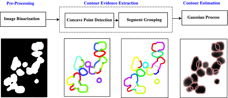
Figure 2: The workflow of the proposed segmentation method includes three major steps: pre-processing, contour evidence extraction and contour segmentation. In pre-processing, the region of the image that is covered by the object of interest is separated from the background. Contour evidence extraction infers the visible parts of the object contours and contour estimation resolves the full contours of an individual object.

The next step called contour evidence extraction involves two separate tasks: contour segmentation and segment grouping. In contour segmentation the contour segments are recovered from a binarized image using concave points detection. In segment grouping, the contour segments which belong to the same objects are grouped by utilizing the branch and bound algorithm Zafari2017BB . Finally, contour evidences are utilized to estimate the full contours of the objects. Once the contour evidence has been obtained contour estimation is carried out to infer the missing parts of the overlapping objects.

3.1 Concave point detection

Concave points detection has a pivotal role in contour segmentation and provides an important cue for further object segmentation (contour estimation). The main goal in concave points detection (CPD) is to find the concavity locations on the objects boundaries and to utilize them to segment the contours of overlapping objects in such way that each contour segment contains edge points from one object only. Although a concave point has a clear mathematical definition, the task of concave points detection from noisy digital images with limited resolution is not trivial. Several methods have been proposed for the problem. These methods can be categorized into three groups: concave chord, skeleton and polygonal approximation based methods.

3.1.1 Concave chord

In concave chord methods, the concave points are the deepest points on the concave region of contours that has the largest perpendicular distance from the corresponding convex hull. The concave regions and their corresponding convex hull chords can be obtained by two approaches as follows. In the method proposed by Farhan et al. farhan2013novel , series of lines are fitted on object contours and concave region are found as a region of contours such that the line joins the two contour points does not reside inside an object. The convex hull chord corresponding to that concave region is a line connecting the sixth adjacent contour point on either side of the current point on the concave region of the object contours. In the method proposed by Kumar et al. chord , the concave points are extracted using the boundaries of concave regions and their corresponding convex hull chords. In this way, the concave points are defined as points on the boundaries of concave regions that have maximum perpendicular distance from the convex hull chord. The boundaries and convex hull are obtained using a method proposed in rosenfeld1985 .

3.1.2 Skeleton

Skeletonization is a thinning process in the binary image that reduces the objects in the image to skeletal remnant such that the essential structure of the object is preserved. The skeleton information along with the object’s contour can also be used to detect the concave points. Given the extracted object contours $C$ and skeleton $SK$ the concave points are determined in two ways. In the method proposed by Samma et al. bnd-skeleton the contour points and skeleton are detected by the morphological operations and then the concave points are identified as the intersections between the skeleton and contour points. In the method proposed by Wang et al. skeleton , the objects are first skeletonized and contours are extracted. Next, for every contour points $c_{i}$ the shortest distance from the skeleton is computed. The concave points are detected as the local minimum on the distance histogram whose value is higher than a certain threshold.

3.1.3 Polygonal approximation

Polygonal approximation is a well-known method for dominant point representation of the digital curves. It is used to reduce the complexity, smooth the objects contours, and avoid detection of false concave points in CPD methods. The majority of the polygonal approximation methods are based on one of the following two approaches: 1) finding a subset of dominant points by local curvature estimation or 2) fitting a curve to a sequence of line segments

The methods that are based on finding a subset of dominant points by local curvature estimation work as follows. Given the sequence of extracted contour points ${C}=\{c_{1},c_{2},...\}$, the dominants points are identified as points with extreme local curvature. The curvature value $k$ for every contour points $c_{i}=(x_{i},y_{i})$ can be obtained by:

$$k=(x_{i}^{\prime}y_{i}^{\prime\prime}-y_{i}^{\prime}x_{i}^{\prime\prime})/(x_{i}^{\prime 2}+y_{i}^{\prime 2})^{3/2}.$$ (1)

The detected dominant points $c_{d,i}\in C_{dom}$ may locate in both concave and convex regions of the objects contours. To detect the dominant points that are concave, various approaches exist. In the method proposed by Wen et al. curv-th the detected dominant points are classified as concave if the value of maximum curvature is larger than a preset threshold value. In the method proposed by Zafari et al. zafari2015segmentation , the dominant points are concave points if the line connecting $c_{d,i+1}$ to $c_{d,i-1}$ does not reside inside the object. In the method proposed by Dai et al. curve-area , the dominant points are qualified as concave points if the value of the triangle area $S$ for the points $c_{d,i+1},c_{d,i},c_{d,i-1}$ is positive and the points are arranged in order of counter-clockwise.

The methods that are based on fitting a curve to a sequence of line segments work as follows. First, a series of lines are fitted to the contour points. Then, the distances from all the points of the object contour located in between the starting and ending points of the line to the fitted lines are calculated. The points whose distance are larger than a preset threshold value considered as the dominant point.

After polygon approximation and dominant points detection, the concave points can be obtained using methods proposed by Bai et al. Bai20092434 and Zhang et al. bubble . In the method proposed by Bai et al. Bai20092434 , the the dominant point $c_{d,i}$ is defined as concave if the concavity value of $c_{d,i}$ is within the range of $a_{1}$ to $a_{2}$ and the line connecting $c_{d,i+1}$ and $c_{d,i-1}$ does not pass through the inside the objects. The concavity value of $c_{d,i}$ is defined as the angle between lines $(c_{d,i-1},c_{d,i})$ and $(c_{d,i+1},c_{d,i})$ as follows:

$$\begin{dcases}\displaystyle\mid\gamma_{1}-\gamma_{2}\mid&\hskip 5.0pt\text{if}\ |\gamma_{1}-\gamma_{2}|<\pi\\ \vspace*{18cm}\pi-|\gamma_{1}-\gamma_{2}|&\text{otherwise},\end{dcases}$$ (2)

where, $\gamma_{1}$ is the angle of the line $(c_{d,i-1},c_{d,i})$ and $\gamma_{2}$ is the angle of the line $(c_{d,i+1},c_{d,i})$ defined as:

$$\gamma_{1}=\tan^{-1}((y_{d,i-1}-y_{d,i})/(x_{d,i-1}-x_{d,i})),$$

$$\gamma_{2}=\tan^{-1}((y_{d,i+1}-y_{d,i})/(x_{d,i+1}-x_{d,i})).$$

In the method proposed by Zhang et al. bubble , the dominant point $c_{d,i}\in C_{dom}$ is considered to be a concave point if $\vv{c_{d,i-1}c_{d,i}}\times\vv{c_{d,i}c_{d,i+1}}$ is positive:

$$\begin{split}{C}_{con}=\{c_{d,i}\in C_{dom}\ :\ \vv{c_{d,i-1}c_{d,i}}\times\vv{c_{d,i}c_{d,i+1}}>0\}\end{split}.$$ (3)

3.2 Proposed method for concave point detection

Most existent concave point detection methods require a threshold value that is selected heuristically  bubble ; Bai20092434 . In fact, finding the optimal threshold value is very challenging, and a unique value may not be suitable for all images in a dataset.

We propose a parameter free concave point detection method that relies on polygonal approximation by fitting the curve with a sequence of line segments. Given the sequence of extracted contour points ${C}=\{c_{1},c_{2},...\}$, first, the dominant points are determined by co-linear suppression. To be specific, every contour point $c_{i}$ is examined for co-linearity, while it is compared to the previous and the next successive contour points. The point $c_{i}$ is considered as the dominant point if it is not located on the line connecting $c_{i-1}=(x_{i-1},y_{i-1})$ and $c_{i+1}=(x_{i+1},y_{i+1})$ and the distance $d_{i}$ from $c_{i}$ to the line connecting $c_{i-1}$ to $c_{i+1}$ is bigger than a pre-set threshold $d_{i}>d_{th}$.

The value of $d_{th}$ is selected automatically using the characteristics of the line as in prasad2012polygonal . In this method, first the line connecting $c_{i-1}$ to $c_{i+1}$ is digitized by rounding the value $(x_{i-1},y_{i-1})$ and $(x_{i+1},y_{i+1})$ to their nearest integer. Next, the angular difference between the numeric tangent of line $c_{i-1}c_{i+1}$ and the digital tangent of line $c^{\prime}_{i-1}c^{\prime}_{i+1}$ is computed as (see Fig. 3):

$$\begin{split}\delta\phi=\tan^{-1}(m)-\tan^{-1}(m^{\prime}),\end{split}$$ (4)

where, $m$ and $m^{\prime}$ are slop of actual and digital line respectively. Then, value of $d_{th}$ is given by:

$$d_{th}=S\delta\phi,$$ (5)

where $S$ is length of actual line.

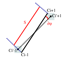
Figure 3: Representation of the actual and the digitized lines.

Finally, the detected dominant points are qualified as concave if they met the criterion by Zhang (Eq. 3) for concave point detection. We referred the proposed concave point detection as Prasad+Zhang Zafari2017 .

3.3 Segment grouping

Due to the overlap between the objects and the irregularities in the object shapes, a single object may produce multiple contour segments. Segment grouping is needed to merge all the contour segments belonging to the same object.

Let $S=\{S_{1},S_{2},...,S_{N}\}$ be an ordered set of $N$ contour segments in a connected component of an image. The aim is to group the contour segments into $M$ subsets such that the contour segments that belong to individual objects are grouped together and $M\leq N$. Let $\omega_{i}$ be the group membership indicator giving the group index to which the contour segment $S_{i}$ belongs to. Denote $\Omega$ be the ordered set of all membership indicators: $\{\omega_{1},\omega_{2},....,\omega_{N}\}$.

The grouping criterion is given by a scalar function $J(\cdot{})$ of $\Omega$ which maps a possible grouping of the given contour segments onto the set of real numbers $\mathbb{R}$. That is, $J$ is the cost of grouping that ideally measures how the grouping $\Omega$ resembles the true contour segments of the objects. The grouping problem for the given set of $S$ is to find the optimal membership set $\Omega^{*}$ such that the grouping criterion (cost of grouping) is minimized:

$$\Omega^{*}=\operatornamewithlimits{argmin}_{\Omega}\ J(\Omega;S).$$ (6)

We formulated the grouping task as a combinatorial optimization problem and solved using the branch and bound (BB) algorithm Zafari2017BB . The BB algorithm can be applied with any grouping criterion $J$. However, the selection of the grouping criterion significantly affects the overall method performance. In this work the grouping criterion is a hybrid cost function consisting of two parts: 1) generic part ($J_{\mathrm{concavity}}$) that encapsulate the general convexity properties of the objects and 2) specific part that encapsulates the properties of objects that are exclusive to a certain application, e.g., symmetry ($J_{\mathrm{symmetry}}$) and ellipticity ($J_{\mathrm{ellipticity}}$). The cost function is defined as follows:

$$J=\underbrace{J_{\mathrm{concavity}}}_{\text{Generic}}\underbrace{+\alpha J_{\mathrm{ellipticity}}+{\beta J_{\mathrm{symmetry}}}}_{\text{Specific}},$$ (7)

where $\alpha$, $\beta$ are the weighting parameters. The generic part encourages the convexity assumption of the objects in order to penalize the grouping of the contour segments belonging to different objects. This is achieved by incorporating a quantitative concavity measure. Given two contour segments $S_{i}$ and $S_{j}$ the generic part of the cost function is defined as follows:

$$\small J_{\mathrm{concavity}}=\begin{cases}1,&$ concave point between $S_{i}$ and $S_{j}$ $\\ (1-\frac{A_{S_{i}\cup S_{j}}}{A_{\mathrm{ch},S_{i}\cup S_{j}}})&\ \text{otherwise},\end{cases}$$ (8)

where ${A_{S_{i}\cup S_{j}}}$ is the area of a region bounded by $S_{i}$, $S_{j}$, and the lines connecting the endpoint of $S_{j}$ to the starting point of $S_{i}$ and the end point of $S_{i}$ to the starting point of $S_{j}$. $A_{\mathrm{ch},S_{i}\cup S_{j}}$ is the upper bound for area of any convex hull with boundary points $S_{i}$ and $S_{j}$. The specific part is adapted to consider the application criteria and certain object properties. Considering the object under examination, several functions can be utilized.

Here, the specific term is formed by the ellipticity and symmetry cost functions. The ellipticity term is defined by measuring the discrepancy between the fitted ellipse and the contour segments bubble . Given the contour segment $S_{i}$ consisting of $n$ points, $S_{i}=\{(x_{k},y_{k})\}_{k=1}^{n}$, and the corresponding fitted ellipse points, $S_{f,i}=\{(x_{f,k},y_{f,k})\}_{k=1}^{n}$, the ellipticity term is defined as follows:

$$\begin{split}\mathrm{J_{ellipticity}}=\frac{1}{n}{\sum}_{k=1}^{n}{\sqrt{(x_{k}-x_{f,k})^{2}+(y_{k}-y_{f,k})^{2}}}.\end{split}$$ (9)

The symmetry term penalizes the resulting objects that are non-symmetry. Let $o_{i}$ and $o_{j}$ be the center of symmetry of the contour segments $S_{i}$ and $S_{j}$ obtained by aggregating the normal vector of the contour segments. The procedure is similar to fast radial symmetry transform frs , but the gradient vectors are replaced by the contour segments’ normal vector. This transform is referred to as normal symmetry transform (NST).

In NST, every contour segment point gives a vote for the plausible radial symmetry at some specific distance from that point. Given the distance value $n$ of the predefined range $[{R}_{min}\ {R}_{max}]$, for every contour segment point $(x,y)$, NST determines the negatively affected pixels ${P}_{-e}$ by

$$\begin{split}&{P}_{-ve}(x,y)=(x,y)-\mathrm{round}{{(}}\frac{\mathrm{\mathbf{n}}(x,y)}{\|\mathrm{\mathbf{n}}(x,y)\|}n{{)}},\\ \end{split}$$ (10)

and increment the corresponding point in the orientation projection image $\mathrm{\mathbf{O}}_{n}$ by $1$. The symmetry contribution $\mathrm{\mathbf{S}}_{n}$ for the radius $n\in[{R}_{min},{R}_{max}]$ is formulated as

$$\begin{split}\mathrm{\mathbf{S}}_{n}(x,y)={{{(}}\frac{|\tilde{\mathrm{\mathbf{O}}}_{n}(x,y)|}{k_{n}}{{)}}}\end{split},$$ (11)

where $k_{n}$ is the scaling factor that normalizes $\mathrm{\mathbf{O}}_{n}$ across different radii. $\tilde{\mathrm{\mathbf{O}}}_{n}$ is defined as

$$\begin{split}\tilde{\mathrm{\mathbf{O}}}_{n}(x,y)=\begin{cases}\mathrm{\mathbf{O}}_{n}(x,y),&\text{if }\mathrm{\mathbf{O}}_{n}(x,y)<k_{n},\\ k_{n},&\text{otherwise}.\end{cases}\end{split}$$ (12)

The full NST transform $\mathrm{\mathbf{S}}$, by which the interest symmetric regions are defined, is given by the average of the symmetry contributions over all the radii $n\in[{R}_{min},{R}_{max}]$ considered as

$$\mathrm{\mathbf{S}}=\frac{1}{|N|}\sum_{n\in[{R}_{min},{R}_{max}]}\mathrm{\mathbf{S}}_{n}.$$ (13)

The center of symmetry $o_{i}$ and $o_{j}$ of the contour segments are estimated as the average locations of the detected symmetric regions in $\mathrm{\mathbf{S}}$. The symmetry term $J_{\mathrm{symmetry}}$ is defined as the Euclidean distance between $o_{i}$ and $o_{j}$ as

$$\begin{split}\mathrm{J_{symmetry}}=|o_{i}-o_{j}|.\end{split}$$ (14)

The distance is normalized to [0,1] according to the maximum diameter of the object.

3.4 Contour estimation

Segment grouping results in, a set of contour points for each object. Due to the overlaps between objects, the contours are not complete and the full contours need to be estimated. Several methods exist to address the contour estimation problem. A widely known approach is Least Square Ellipse Fitting (LESF) fitzgibbon1999direct . The purpose of LESF is to computing the ellipse parameters by minimizing the sum of squared algebraic distances from the known contour evidences points to the ellipse. The method is highly robust and easy to implement, however, it fails to accurately approximate complicated non-elliptical shapes.

Closed B-splines is another group of methods for the contour estimation. In npa , the B-Splines with Expectation Maximization (BS) algorithm was used to infer the full contours of predefined possible shapes. The reference shape and the parameters of the B-spline of the object are comprised in the Gaussian mixture model. The inference of the curve parameters, namely shape properties and the parameters of B-spline, from this probabilistic model is addressed through the Expectation Conditional Maximization (ECM) algorithm meng1993ecm . The accuracy of the method depends on the size and diversity of the set of reference shapes and gets low if the objects highly overlap.

3.5 Proposed method for contour estimation

To address the issues with the existing methods, we propose a Gaussian process based method for the contour estimation. Gaussian processes (GP) are nonparametric kernel-based probabilistic models that have been used in several machine learning applications such as regression, prediction, and contour estimation martin2005use ; RICHARDSON2017209 . In  YANG2018387 a GP model based on charging curve is proposed for state-of-health (SOH) estimation of lithium-ion battery. In pmlr-v28-wilson13 GP is applied for pattern discovery and extrapolation. In  7274766 a regression method based on the GP is proposed for prediction of wind power.

The primary assumption in GP is that the data can be represented as a sample from a multivariate Gaussian distribution. GP can probabilistically estimate the unobserved data point, $f^{*}$, based on the observed data, $f$, assuming that the both observed data point and unobserved data can be represented as a sample from a multivariate Gaussian distribution

$$\begin{pmatrix}f\\ f^{*}\\ \end{pmatrix}=\mathcal{N}\begin{pmatrix}\begin{pmatrix}\mu_{\mathbf{x}}\\ \mu_{\mathbf{x}^{*}}\\ \end{pmatrix},\begin{pmatrix}\mathrm{\mathbf{K}}_{\mathbf{x\mathbf{x}}}&\mathrm{\mathbf{k}}_{\mathbf{x^{*}}}^{T}\\ \mathrm{\mathbf{k}}_{\mathbf{x^{*}}}&\mathrm{\mathbf{K}}_{\mathbf{x^{*}\mathbf{x^{*}}}}\\ \end{pmatrix}\end{pmatrix},$$ (15)

where $\mathbf{K}$ is the $n\times n$ covariance matrix and $\mathrm{\mathbf{k}}_{\mathbf{x}^{*}}$ is an $n\times 1$ vector containing the covariances between $x^{*}$ and $x_{1},x_{2},\ldots,x_{n}$ given by

$$[\mathbf{K}]_{ij}=\kappa(x_{i},x_{j}),$$ (16)

and

$$\mathbf{k}_{\mathbf{x}^{*}}=[\kappa(x_{1},x^{*}),\kappa(x_{2},x^{*}),\ldots,\kappa(x_{n},x^{*})]^{T}.$$ (17)

$\kappa(.,.)$ is defined by the Matern covariance function rasmussen2006gaussian as follows:

$$\begin{split}\kappa(x_{i},x_{j})=\frac{2^{1-v}}{\Gamma(v)}(\frac{\sqrt{2v}|d|}{l})^{v}K_{v}(\frac{\sqrt{2v}|d|}{l})\end{split},$$ (18)

where $x_{i}$, $x_{j}$, $i\neq j$, $i=1,2,\ldots,n$ are a pair of data point, $l$ is the characteristic length scale, $d$ is the Euclidean distance between the points $x_{i}$ and $x_{j}$ and $K_{v}$ is the modified Bessel function of order $v$. The most common choices for $v$ are $v=3/2$ and $v=5/2$ that are denoted by Matern 3/2 and Matern 5/2.

Let $D~{}=~{}\{(x_{i},y_{i})\}_{i=1}^{n}$ be the input data, $\mathbf{x}=[x_{1},\ldots,x_{n}]^{T}$ be the input vector and $\mathbf{y}=[y_{1},\ldots,y_{n}]^{T}$ be the corresponding observations vector given by a latent function $f(.)$. GP assumes the latent function comes from a zero-mean Gaussian and the observations are modeled by

$$\begin{split}{y_{i}}=f({x_{i}})+\epsilon_{i},\quad\epsilon_{i}\sim\mathcal{N}(0,\sigma^{2}).\end{split}$$ (19)

Given the $D,f$ and a new point $\mathbf{x^{*}}$, the GP defines the posterior distribution of the latent function $f(.)$ at the new point $f(\mathbf{x}^{*})$ as Gaussian and obtains the best estimate for $\mathbf{x^{*}}$ by the mean and variance of the posterior distribution as follows:

$$\begin{split}p(f^{*}|\mathbf{x}^{*},{D})=\mathcal{N}({f^{*}}|{\mu_{\mathbf{x}^{*}}},{\sigma^{2}_{\mathbf{x}^{*}}}),\end{split}$$ (20)

where

$$\mathbf{\mu}_{\mathbf{x^{*}}}=\mathbf{k}_{\mathbf{x}^{*}}^{T}\mathbf{K}_{\mathbf{x}\mathbf{x}}^{-1}\mathbf{y},$$ (21)

and

$$\mathbf{\sigma}_{\mathbf{x^{*}}}^{2}=\mathbf{K}_{\mathbf{x^{*}}\mathbf{x^{*}}}-\mathbf{k}_{\mathbf{x}^{*}}^{T}\mathbf{K}_{\mathbf{x}\mathbf{x}}^{-1}\mathbf{k}_{\mathbf{x}^{*}}.$$ (22)

To exploit GP for the task of contour estimation and to limit the interpolation interval to a finite domain, the polar representation of contour evidence is needed. Polar representation has three advantages. First, it limits the interpolation interval to a finite domain of $[0,2\pi]$, second, it exploits the correlation between the radial and angular component, and third, it reduces the number of dimensions compared to GP based on parametric Cartesian representation.

In GP with polar form (GP-PF), the contour evidence points are represented as a function of the radial and angular components. Given the contour evidence points $x$ and $y$, their polar transform is defined as follows:

$$\begin{split}{\theta}&=\arctan{\left(\frac{y}{x}\right)},\\ r&=\sqrt{x^{2}+y^{2}}.\end{split}$$ (23)

Here, the angular component $\theta$ is considered to be the input to the GP and the radial $r$ as the corresponding observations described by the latent function $r=f(\theta)$. To enforce the interpolation to a closed periodic curve estimation such that $f(\theta)=f(\theta+2\pi)=r$, the input set is defined over the finite domain $\theta^{*}\in[0,2\pi]$ as $D=\{(\theta_{i},r_{i})\}_{i=1}^{n}\cup\{(\theta_{i}+2\pi,r_{i}),...\}_{i=1}^{n}$. The best estimate for $r^{*}$ is obtained by the mean of the distribution

$$\mathbf{\mu}_{\theta^{*}}=\mathbf{k}_{{\theta}^{*}}^{T}\mathbf{K}_{{\theta}{\theta}}^{-1}\mathrm{\mathbf{r}}.$$ (24)

The GP-PF method is summarized in Algorithm 1.

Input: Contour evidence coordinates $x$, $y$.

Output: Estimated objects’ full contour points $x^{*}$, $y^{*}$.

Parameters: Covariance function $k$

1. Perform mean centering for $x$, $y$ by subtracting their mean from all their values.

2. Retrieve polar coordinates $\theta$, $r$ from $x$, $y$ using Eq. [23].

3. Define the input set and the corresponding output for the observed contour points as

$D=\{(\theta_{i},r_{i})\}_{i=1}^{n}\cup\{(\theta_{i}+2\pi,r_{i}),...\}_{i=1}^{n}$.

Define the new input set for unobserved contour points by $\theta^{*}\in[0,2\pi]$. 5. Estimate the covariance function, $K_{\theta^{*}\theta^{*}},k_{\theta^{*}},K_{\theta\theta}$ using Eq. [18]. 6. Predict the output, $r^{*}$, on the new input set, $\theta^{*}$, using the predictive mean using Eq. [24]. 7. Transform $\theta^{*}$, $r^{*}$ from polar to Cartesian coordinates $x^{*}$, $y^{*}$.

Algorithm 1 Contour Estimation by GP-PF

4 Experiments

This section presents the data, the performance measures, and the results for the concave points detection, contour estimation, and segmentation.

4.1 Data

The experiments were carried out using one synthetically generated dataset and one dataset from a real-world application.

The synthetic dataset (see Fig. 4(a)) consists of images with overlapping ellipse-shape objects that are uniformly randomly scaled, rotated, and translated. Three subsets of images were generated to represent different degrees of overlap between objects. The dataset consists of 150 sample images divided into three classes of overlap degree. The maximum rates of the overlapping area allowed between two objects are 40%, 50%, and 60%, respectively, for the first, second, and third subset. Each subset of images in the dataset contains 50 images of 40 objects. The minimum and maximum width and length of the ellipses are 30, and 45 pixels. The image size is $300\times 400$ pixels.

The real dataset (nanoparticles dataset) contains nanoparticles images captured using transmission electron microscopy (see Fig. 4(b)). In total, the dataset contains 11 images of $4008\times 2672$ pixels. Around 200 particles were marked manually in each image by an expert. In total the dataset contains 2200 particles.The annotations consist of manually drawn contours of the particles. This information was also used to determine the ground truth for concave points. Since not all the particles were marked, a pre-processing step was applied to eliminate the unmarked particles from the images. It should be noted that the images consist of dark objects on a white background and, therefore, pixels outside the marked objects can be colored white without making the images considerably easier to analyze.

(a)	(b)

Figure 4: Example images from the datasets studied: (a) Synthetic dataset with the maximum overlap of 40%; (b) Nanoparticles dataset.

4.2 Performance Measures

To evaluate the method performance and to compare the methods, the following performance measures were used: The detection performance for both concave points and objects were measured using True Positive Rate (TPR), Positive Predictive Value (PPV), and Accuracy (ACC) defined as follows:

$$TPR =\frac{TP}{TP+FN},$$ (25)

$$PPV =\frac{TP}{TP+FP},$$ (26)

$$ACC =\frac{TP}{TP+FP+FN},$$ (27)

where True Positive (TP) is the number of correctly detected concave points or segmented objects, False Positive (FP) is the number of incorrectly detected concave points or segmentation results, and False Negative (FN) is the number of missed concave points or objects. To determine whether a concave point was correctly detected (TP), the distance to the ground truth concave points was computed and the decision was made using a predefined threshold value. The threshold value was set to 10 pixels. Moreover, the average distance (AD) from detected concave points to the ground truth concave points was measured for the concave points detection. To decide whether the segmentation result was correct or incorrect, Jaccard Similarity coefficient (JSC) Choi10asurvey was used. Given a binary map of the segmented object $O_{s}$ and the ground truth particle $O_{g}$, JSC is computed as

$$JSC=\frac{O_{s}\cap O_{g}}{O_{s}\cup O_{g}}.$$ (28)

The threshold value for the ratio of overlap (JSC threshold) was set to 0.6. The average JSC (AJSC) value was also used as a performance measure to evaluate the segmentation performance.

4.3 Parameter selection

The proposed method requires the following major parameters.

Weighting parameters $\alpha$, and $\beta$ define to what extent the ellipticity and symmetry features must be weighted in the computation of the grouping cost $J$. A lower value of $\alpha$ and $\beta$ emphasizes non-ellipticity and non-symmetry features where higher values ensure that objects have perfect elliptical symmetry shapes. This parameter is useful when the objects are not perfectly elliptical. In this work, the weighting parameters $\alpha$, and $\beta$ were set to $0.1$ and $0.9$ to obtain the highest performance of segment grouping.

Type of the covariance function determines how the covariance function measure the similarity of any two points of the data, and specifies the desired form of the output function and affects the final contour estimation result. In this work, the contour estimation is performed using the GP-PF method with the Matern 5/2 covariance function as a more flexible and general one.

The parameters of the concave points detection methods were set experimentally to obtain the best possible result for each method.

4.4 Results

4.4.1 Concave points detection

The results of the concave points detection methods applied to real nanoparticles and synthetic datasets are presented in Tables 1 and 2, respectively. The results have been reported with the optimal parameters setup for each listed methods. The chosen nanoparticle dataset is challenging for CPD experiments since it contains objects with noisy boundaries. Here, the noise includes the small or large scale fluctuations on the object boundaries that can affect the performance of the concave points detection methods. The results on the nanoparticles dataset (Table 1) show that the Prasad+Zhang method outperforms the others with the highest TPR and ACC values and the competitive PPV and AD values. From the results with the synthetic dataset (Table 2) it can be seen that Prasad+Zhang achieved the highest value of ACC. Zhang bubble scored the highest values of TPR and AD, but it suffers from the low values of PPV and ADD. This is because the method produces a large number of false concave points. Comparing the Zhang bubble and Prasad+Zhang Zafari2017 CPD methods shows the advantage of the proposed parameter selecting strategy in concave points detection that makes the Prasad+Zhang method a more robust in presence of objects with noisy boundaries. In terms of PPV, Zafari zafari2015segmentation and Kumar concavity ranked the highest. However, these approaches tend to underestimate the number of concave points as they often fail to detect the concave points at a low depth of concave regions. Considering all the scores together, the results obtained from the synthetic dataset showed that the Prasad+Zhang method achieved the best performance.

The results presented in Tables 1 and 2 were obtained by a fixed distance threshold value of 10 pixels. To check the stability of the results with respect to distance threshold ($\rho_{1}$), the distance threshold was examined by the nanoparticles datasets. The effect of $\rho_{1}$ on the TPR, PPV and ACC scores captured with the concave point detection methods are presented in Fig. 5. As it can be seen, the Prasad+Zhang method achieved the highest score of TPR and ACC regardless of the selected threshold. It is worth mentioning that at low values of $\rho_{1}$, the Prasad+Zhang method outperforms all methods with respect to PPV. This is clearly since the Prasad+Zhang method can detect the concave points more precisely.

Methods	TPR	PPV	ACC	AD	Time
	[%]	[%]	[%]	[pixel]	(s)
Prasad+Zhang Zafari2017	96	90	87	1.47	0.50
Zhang bubble	84	38	35	1.42	2.28
Bai Bai20092434	79	40	36	1.55	2.52
Zafari zafari2015segmentation	65	95	64	2.30	2.48
Wen curv-th	94	51	50	1.97	2.13
Dai curve-area	54	87	50	2.84	2.50
Samma bnd-skeleton	80	84	70	2.28	2.95
Wang skeleton	65	58	44	2.37	4.95
Kumar chord	33	94	31	3.09	8.17
Farhan farhan2013novel	77	15	14	2.09	8.82

Table 1: Comparison of the performance of concave points detection methods on the nanoparticles dataset.

Methods	Overlapping	TPR	PPV	ACC	AD
	[%]	[%]	[%]	[%]	[pixel]
Prasad+Zhang Zafari2017	40	97	97	94	1.47
Zhang bubble	40	98	37	37	1.25
Bai Bai20092434	40	92	46	44	1.34
Zafari zafari2015segmentation	40	81	98	80	2.04
Wen curv-th	40	97	61	60	1.75
Dai curve-area	40	71	97	70	2.58
Samma bnd-skeleton	40	75	83	65	2.20
Wang skeleton	40	87	86	76	1.87
Kumar chord	40	64	98	62	2.64
Farhan farhan2013novel	40	91	18	18	1.77
Prasad+Zhang Zafari2017	50	97	96	93	1.50
Zhang bubble	50	96	38	38	1.25
Bai Bai20092434	50	86	47	44	1.34
Zafari zafari2015segmentation	50	77	98	76	2.08
Wen curv-th	50	94	62	60	1.81
Dai curve-area	50	68	97	66	2.57
Samma bnd-skeleton	50	73	83	63	2.24
Wang skeleton	50	83	86	74	1.95
Kumar chord	50	60	98	59	2.62
Farhan farhan2013novel	50	87	19	18	1.81
Prasad+Zhang Zafari2017	60	94	96	91	1.51
Zhang bubble	60	96	40	39	1.31
Bai Bai20092434	60	82	37	43	1.47
Zafari zafari2015segmentation	60	73	98	73	2.13
Wen curv-th	60	91	64	60	1.79
Dai curve-area	60	63	98	62	2.61
Samma bnd-skeleton	60	67	82	59	2.26
Wang skeleton	60	80	88	72	1.96
Kumar chord	60	58	98	57	2.71
Farhan farhan2013novel	60	82	19	19	1.91

Table 2: Comparison of the performance of concave points detection methods on the synthetic dataset.

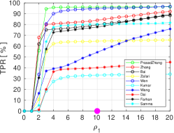
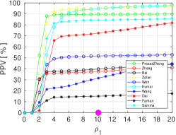
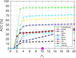
(a)	(b)	(c)

Figure 5: Performance of concave detection methods with different values of the distance threshold ($\rho_{1}$) in the nanoparticles dataset: (a) TPR; (b) PPV; (c) ACC.

Fig. 6 shows example results of the concave points detection methods applied to a patch of a nanoparticles image. It can be seen that while Zafari zafari2015segmentation , Dai curve-area , Kumar concavity and Samma bnd-skeleton suffer from false negatives and Zhang bubble , Bai Bai20092434 , Wen curv-th and Farhan farhan2013novel suffer from false positives, Prasad+Zhang Zafari2017 suffers from neither false positives nor false negatives.

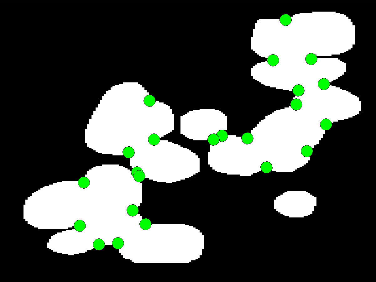
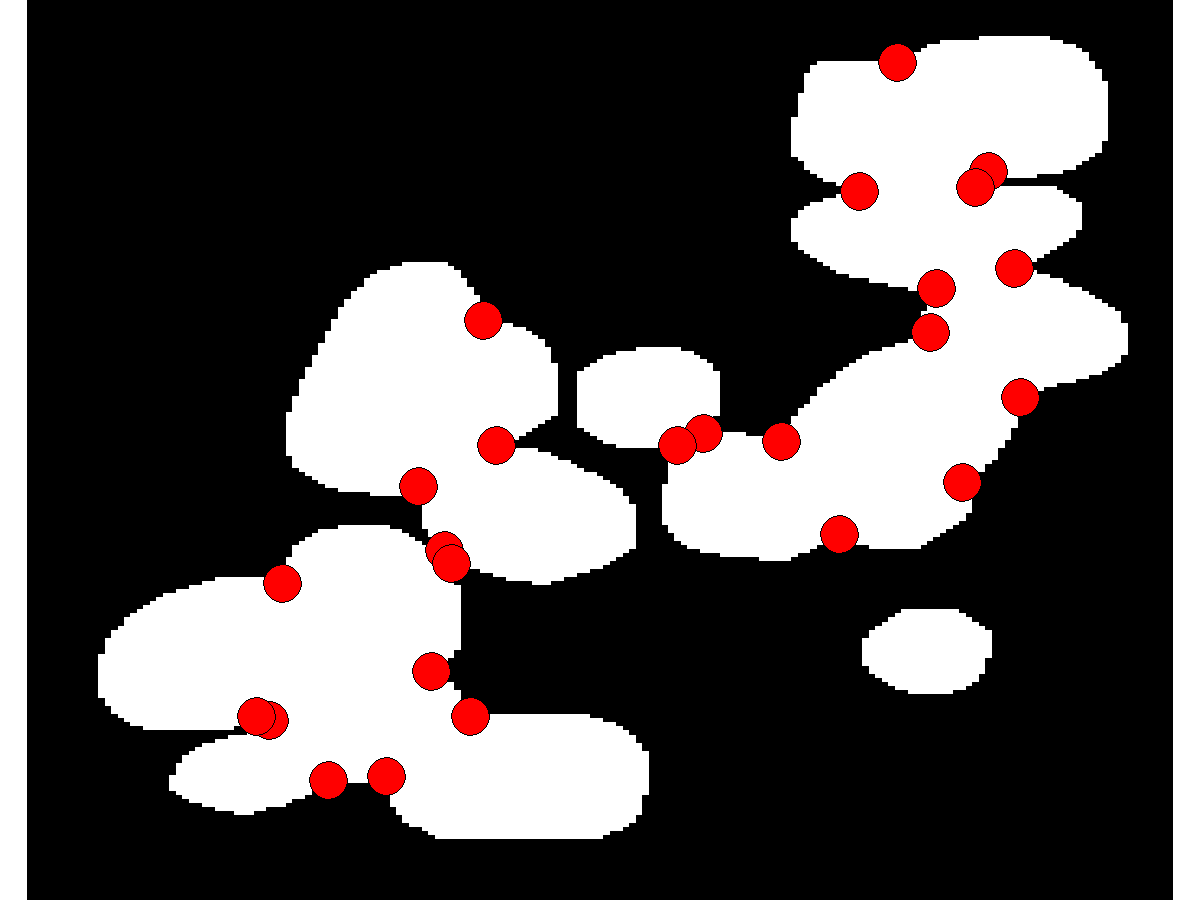
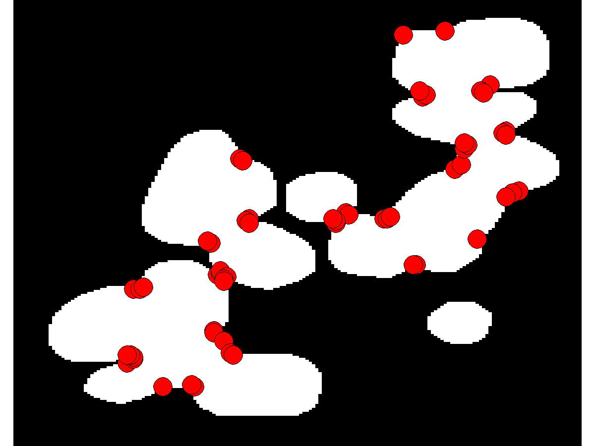
(a)	(b)	(c)

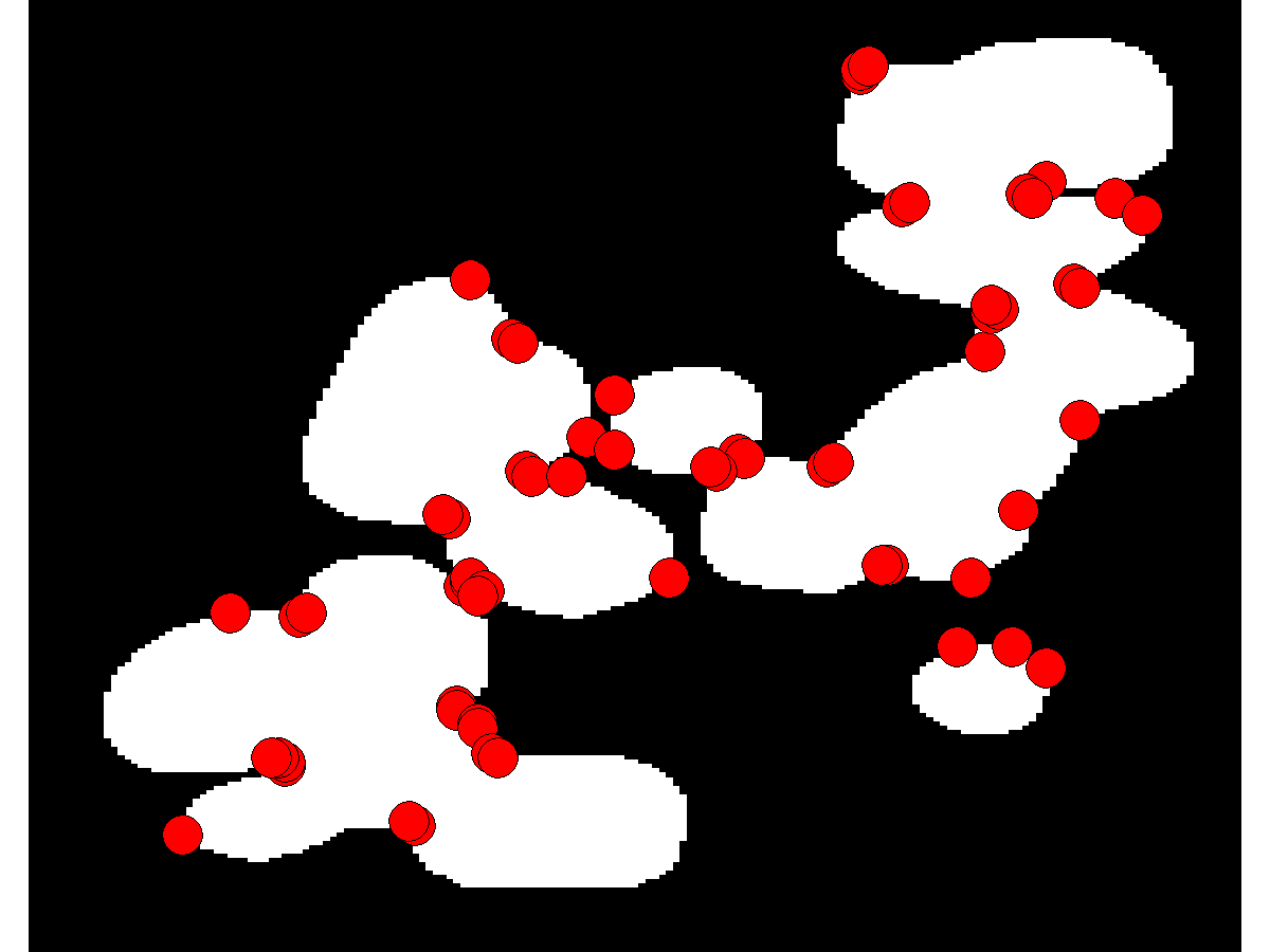
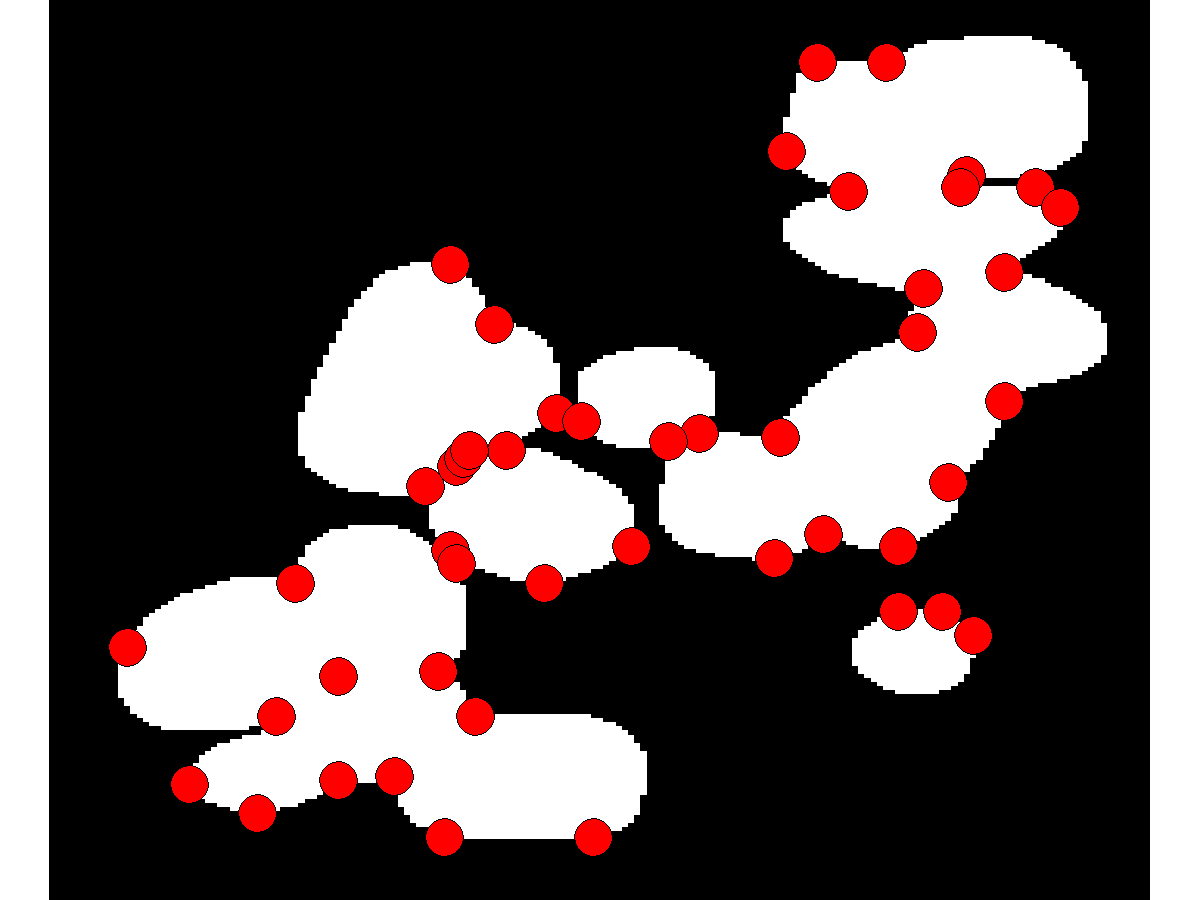
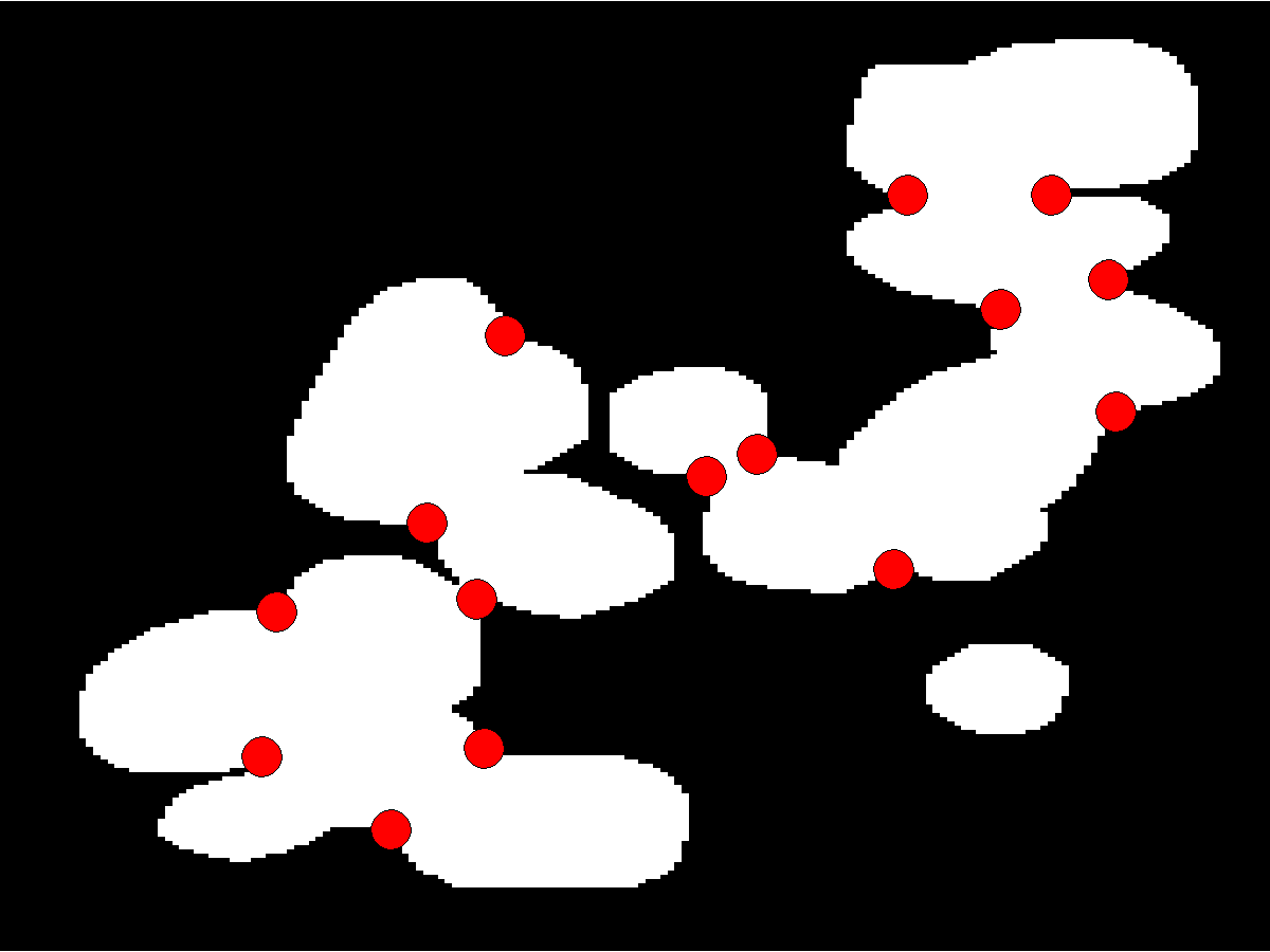
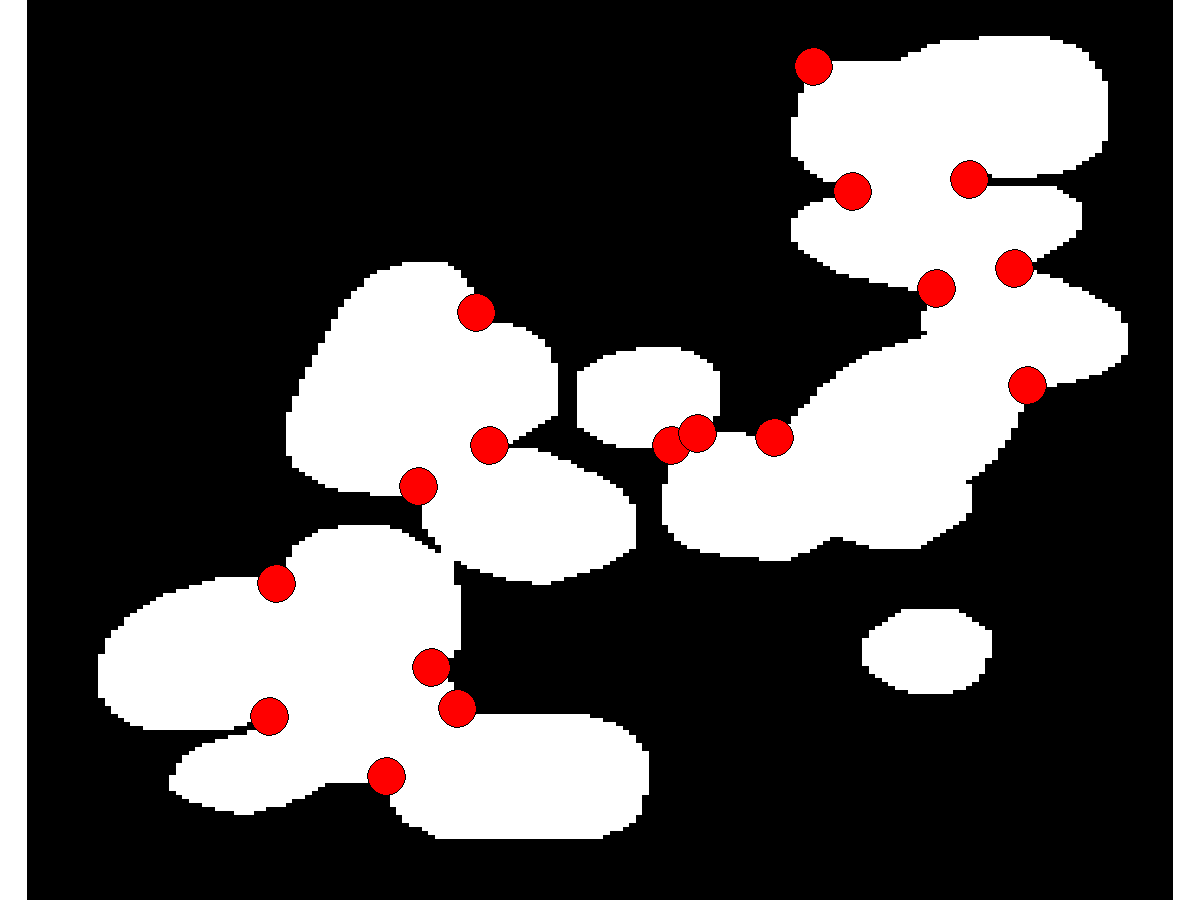
(d)	(e)	(f)	(g)

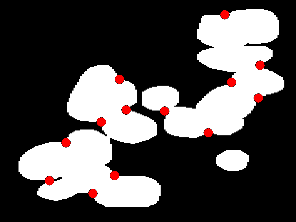
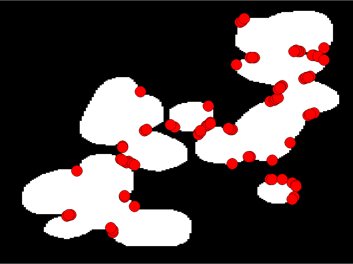
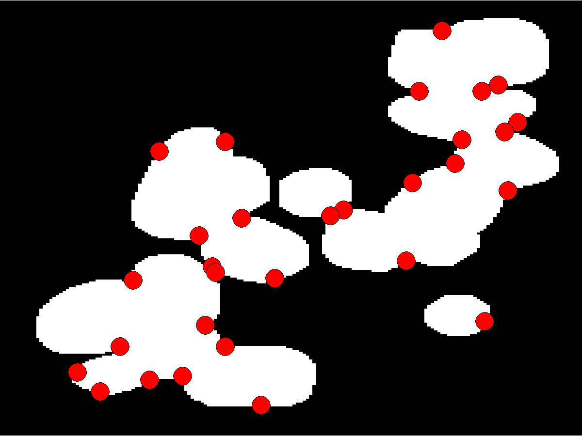
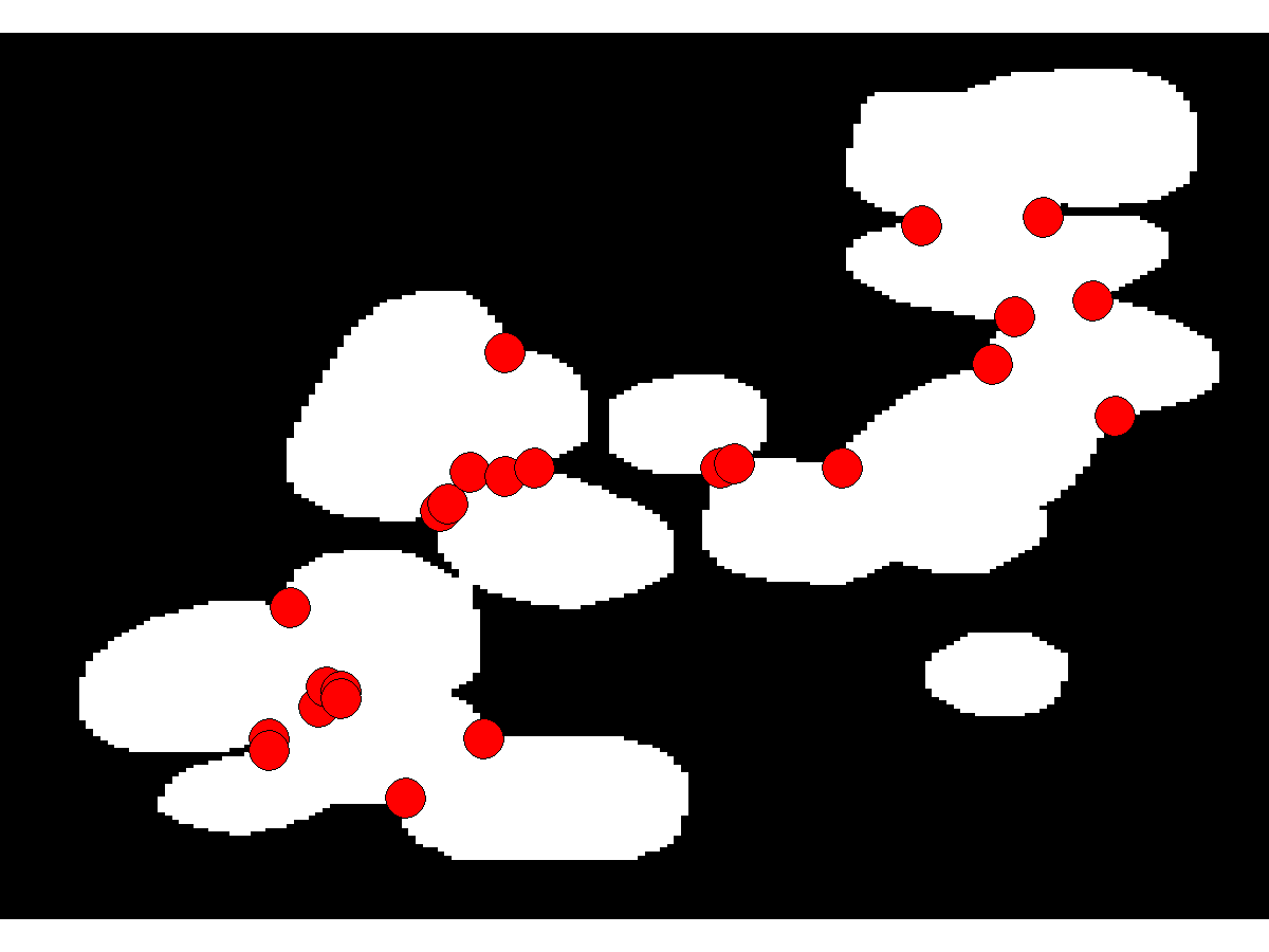
(h)	(i)	(j)	(k)

Figure 6: Comparison of the performance of the concave points detection methods on the nanoparticles dataset: (a) Ground Truth; (b) Prasad+Zhang Zafari2017 ; (c) Zhang bubble ; (d) Bai Bai20092434 ; (e) Wen curv-th ; (f) Zafari zafari2015segmentation ; (g) Dai curve-area ; (h) Kumar concavity ; (i) Farhan farhan2013novel ; (j) Wang skeleton ; (k) Samma bnd-skeleton .

4.4.2 Contour estimation

Tables 3 and 4 show the results of contour estimation with the proposed GP-PF using various types of commonly used covariance functions on the nanoparticles dataset using both the ground truth contour evidences and the contour evidences obtained using the proposed contour evidence extraction method. As it can be seen the Matern family outperforms the other covariance functions with both the ground truth and obtained contour evidences.

Methods	TPR	PPV	ACC	AJSC
	[%]	[%]	[%]	[%]
Matern 3/2	96	96	92	89
Matern 5/2	96	97	93	89
Squared exponential	91	92	84	85
Rational quadratic	95	96	92	88

Table 3: The performance of the proposed GP-PF method with different covariance functions on the ground truth contour evidences.

Methods	TPR	PPV	ACC	AJSC
	[%]	[%]	[%]	[%]
Matern 3/2	87	83	74	87
Matern 5/2	87	83	74	87
Squared exponential	83	78	68	83
Rational quadratic	87	82	73	85

Table 4: The performance of the proposed GP-PF method with different covariance functions on the obtained contour evidences.

Methods	TPR	PPV	ACC	AJSC
	[%]	[%]	[%]	[%]
GP-PF	96	96	92	90
BS	92	92	86	89
LESF	94	95	89	88

Table 5: The performance of the contour estimation methods on the ground truth contour evidences.

To demonstrate the effect of the more accurate contour estimation on the segmentation of partially overlapping objects, the performance of the GP-PF method was compared to the BS and the LESF methods on the nanoparticle dataset. Table 5 shows the segmentation results produced by the contour estimation methods applied to the ground truth contour evidences and Table 6 presents their performance with the obtained contour evidences.

Methods	TPR	PPV	ACC	AJSC
	[%]	[%]	[%]	[%]
GP-PF	87	83	74	87
BS	82	76	66	87
LESF	85	83	71	87

Table 6: The performance of the contour estimation methods on the obtained contour evidences.

The results show the advantage of the proposed GP-PF method over the other methods when applied to the ground truth contour evidences. In all terms the proposed contour estimation method achieved the highest performance. The results on the obtained contour evidences (Table 6) confirm the out-performance of the GP-PF method over the others with the highest values.

In general, the LESF contour estimation takes advantage of objects with an elliptical shape which can lead to desirable contour estimation if the objects are in the form of ellipses. However, in situations where objects are not close to elliptical shapes, the method fails to estimate the exact contour of the objects. The BS contour estimation is not limited to specific object shapes, but requires to learn many contour functions with prior shape information. The proposed Gaussian process contour estimation can resolve the actual contour of the objects without any strict assumption on the object’s shape.

Fig. 7 shows example results of contour estimation methods applied to a slice of nanoparticles dataset.

(a)	(b)
(c)	(d)

Figure 7: Comparison of the performance of contour estimation methods on the ground truth contour evidences: (a) Ground truth full contour; (b) GP-PF; (c) BS; (d) LESF.

It can be seen that BS tends to underestimate the shape of the objects. With small contour evidences, the BS method results in a small shape while LESF can result in larger shapes. The proposed GP-PF method estimates the objects boundaries more precisely.

Figs. 8 and 9 show the effect of the Jaccard similarity threshold on the TPR, PPV, and ACC scores with the proposed and competing contour estimation methods. As expected, the segmentation performance of all methods degrades when the JSC threshold is increased. However, the threshold value has only the minor effect on the ranking order of the methods and the proposed contour estimation method outperforms the other methods with higher JSC threshold values.

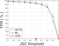
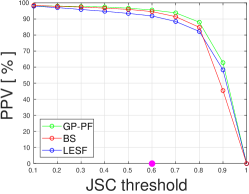
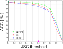
(a)	(b)	(c)

Figure 8: Evaluation results for the contour estimation methods with the different JSC thresholds value applied to the ground truth contour evidences: (a) TPR; (b) PPV; (c) ACC.

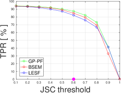
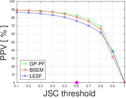
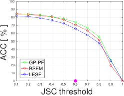
(a)	(b)	(c)

Figure 9: Evaluation results for the contour estimation methods with the different JSC threshold values applied to the obtained contour evidences: (a) TPR; (b) PPV; (c) ACC.

4.4.3 Segmentation of overlapping convex objects

The proposed method is organized in a sequential manner where the performance of each step directly impact the performance of the next step. In each step, all the potential methods are compared and the best performer is selected. The performance of the full proposed segmentation method using the Prasad+Zhang concave points detection and the proposed GP-PF contour estimation methods was compared to three existing methods: seed point based contour evidence extraction and contour estimation (SCC) 7300433 , nanoparticles segmentation (NPA) npa , and concave-point extraction and contour segmentation (CECS) bubble . These methods are particularly chosen as previously applied for segmentation of overlapping convex objects. Fig. 10 shows an example of segmentation result for the proposed method.

(a)	(b)

Figure 10: An example of the proposed method segmentation result on the nanoparticles dataset: (a) Ground truth; (b) Proposed method.

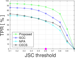
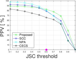
(a)	(b)	(c)

Figure 11: Evaluation results for the segmentation methods with the different JSC threshold values: (a) TPR; (b) PPV; (c) ACC.

The corresponding performance statistics of the competing methods applied to the nanoparticles dataset are shown in Table 7. As it can be seen, the proposed method outperformed the other four methods with respect to TPR, PPV, ACC, and AJSC. The highest TPR, PPV, and ACC indicates its superiority with respect to the resolved overlap ratio.

Fig 11 shows the effect of the Jaccard similarity threshold on the TPR, PPV, and ACC scores with the proposed segmentation and competing methods. As it can be seen, the performance of all segmentation methods degrades when the JSC threshold is increased, and the proposed segmentation method outperforms the other methods especially with higher JSC threshold values.

Methods	TPR	PPV	ACC	AJSC
	[%]	[%]	[%]	[%]
Proposed	87	83	74	87
SCC	74	79	62	82
NPA	57	80	50	81
CECS	58	66	45	83

Table 7: Comparison of the performance of the segmentation methods on the nanoparticles dataset.

5 Conclusions

This paper presented a method to resolve overlapping convex objects in order to segment the objects in silhouette images. The proposed method consisted of three main steps: pre-processing to produce binarized images, contour evidence extraction to detect the visible part of each object, and contour estimation to estimate the final objects contours. The contour evidence extraction is performed by detecting concave points and solving the contour segment grouping using the branch and bound algorithm. Finally, the contour estimation is performed using Gaussian process regression. To find the best method for concave points detection, comprehensive evaluation of different approaches was made. The experiments showed that the proposed method achieved high detection and segmentation accuracy and outperformed four competing methods on the dataset of nanoparticles images. The proposed method relies only on edge information and can be applied also to other segmentation problems where the objects are partially overlapping and have an approximately convex shape.

References

- (1) Al-Kofahi, Y., Lassoued, W., Lee, W., Roysam, B.: Improved automatic detection and segmentation of cell nuclei in histopathology images. IEEE Transactions on Biomedical Engineering 57(4), 841–852 (2010)
- (2) Ali, S., Madabhushi, A.: An integrated region-, boundary-, shape-based active contour for multiple object overlap resolution in histological imagery. IEEE Transactions on Medical Imaging 31(7), 1448–1460 (2012)
- (3) Angulo, J., Jeulin, D.: Stochastic watershed segmentation. In: Proceedings of the 8th International Symposium on Mathematical Morphology, pp. 265–276 (2007)
- (4) Arteta, C., Lempitsky, V., Noble, J.A., Zisserman, A.: Learning to detect partially overlapping instances. In: Proceedings of the IEEE Conference on Computer Vision and Pattern Recognition (CVPR), pp. 3230–3237 (2013)
- (5) Bai, X., Sun, C., Zhou, F.: Splitting touching cells based on concave points and ellipse fitting. Pattern Recognition 42(11), 2434 – 2446 (2009)
- (6) Bernardis, E., Stella, X.Y.: Finding dots: Segmentation as popping out regions from boundaries. In: Proceedings of the IEEE Conference on the Computer Vision and Pattern Recognition (CVPR), pp. 199–206 (2010)
- (7) Canny, J.: A computational approach to edge detection. IEEE Transactions on Pattern Analysis and Machine Intelligence 8(6), 679–698 (1986)
- (8) Chang, H., Han, J., Borowsky, A., Loss, L., Gray, J.W., Spellman, P.T., Parvin, B.: Invariant delineation of nuclear architecture in glioblastoma multiforme for clinical and molecular association. IEEE Transactions on Medical Imaging 32(4), 670–682 (2013)
- (9) Chen, C., Wang, W., Ozolek, J.A., Rohde, G.K.: A flexible and robust approach for segmenting cell nuclei from 2d microscopy images using supervised learning and template matching. Cytometry Part A 83(5), 495–507 (2013)
- (10) Cheng, J., Rajapakse, J.: Segmentation of clustered nuclei with shape markers and marking function. IEEE Transactions on Biomedical Engineering, 56(3), 741–748 (2009)
- (11) Choi, S.S., Cha, S.H., Tappert, C.C.: A survey of binary similarity and distance measures. Journal of Systemics, Cybernetics and Informatics 8(1), 43–48 (2010)
- (12) Dai, J., Chen, X., Chu, N.: Research on the extraction and classification of the concave point from fiber image. In: IEEE 12th International Conference on Signal Processing (ICSP), pp. 709–712 (2014)
- (13) Daněk, O., Matula, P., Ortiz-de Solórzano, C., Muñoz-Barrutia, A., Maška, M., Kozubek, M.: Segmentation of touching cell nuclei using a two-stage graph cut model. In: A.B. Salberg, J. Hardeberg, R. Jenssen (eds.) Image Analysis, Lecture Notes in Computer Science, vol. 5575, pp. 410–419 (2009)
- (14) Erdil, E., Mesadi, F., Tasdizen, T., Cetin, M.: Disjunctive normal shape boltzmann machine. In: Proceedings of the IEEE International Conference on Acoustics, Speech and Signal Processing (ICASSP), pp. 2357–2361 (2017)
- (15) Eslami, S.M.A., Heess, N., Williams, C.K.I., Winn, J.: The shape boltzmann machine: A strong model of object shape. International Journal of Computer Vision 107(2), 155–176 (2014)
- (16) Farhan, M., Yli-Harja, O., Niemistö, A.: A novel method for splitting clumps of convex objects incorporating image intensity and using rectangular window-based concavity point-pair search. Pattern Recognition 46(3), 741–751 (2013)
- (17) Fitzgibbon, A., Pilu, M., Fisher, R.B.: Direct least square fitting of ellipses. IEEE Transactions on Pattern Analysis and Machine Intelligence 21(5), 476–480 (1999)
- (18) Hearst, M.A., Dumais, S., Osman, E., Platt, J., Scholkopf, B.: Support vector machines. Intelligent Systems and Their Applications 13(4), 18–28 (1998)
- (19) Jung, C., Kim, C.: Segmenting clustered nuclei using h-minima transform-based marker extraction and contour parameterization. IEEE Transactions onBiomedical Engineering 57(10), 2600–2604 (2010)
- (20) Kothari, S., Chaudry, Q., Wang, M.: Automated cell counting and cluster segmentation using concavity detection and ellipse fitting techniques. In: IEEE International Symposium on Biomedical Imaging, pp. 795–798 (2009)
- (21) Kumar, S., Ong, S.H., Ranganath, S., Ong, T.C., Chew, F.T.: A rule-based approach for robust clump splitting. Pattern Recognition 39(6), 1088–1098 (2006)
- (22) Law, Y.N., Lee, H.K., Liu, C., Yip, A.: A variational model for segmentation of overlapping objects with additive intensity value. IEEE Transactions on Image Processing 20(6), 1495–1503 (2011)
- (23) Lou, X., Koethe, U., Wittbrodt, J., Hamprecht, F.: Learning to segment dense cell nuclei with shape prior. In: IEEE Conference on Computer Vision and Pattern Recognition (CVPR), pp. 1012–1018 (2012)
- (24) Loy, G., Zelinsky, A.: Fast radial symmetry for detecting points of interest. IEEE Transactions on Pattern Analysis and Machine Intelligence 25(8), 959–973 (2003)
- (25) Mao, K.Z., Zhao, P., Tan, P.H.: Supervised learning-based cell image segmentation for p53 immunohistochemistry. IEEE Transactions on Biomedical Engineering 53(6), 1153–1163 (2006)
- (26) Martin, J.D., Simpson, T.W.: Use of kriging models to approximate deterministic computer models. American Institute of Aeronautics and Astronautics Journal(AIAA J) 43(4), 853–863 (2005)
- (27) Meng, X.L., Rubin, D.B.: Maximum likelihood estimation via the ecm algorithm: A general framework. Biometrika 80(2), 267–278 (1993)
- (28) Otsu, N.: A threshold selection method from gray-level histograms. Automatica 11(285-296), 23–27 (1975)
- (29) Park, C., Huang, J.Z., Ji, J.X., Ding, Y.: Segmentation, inference and classification of partially overlapping nanoparticles. IEEE Transactions on Pattern Analysis and Machine Intelligence 35(3), 669–681 (2013)
- (30) Prasad, D.K., Leung, M.K.: Polygonal representation of digital curves. INTECH Open Access Publisher (2012)
- (31) Quelhas, P., Marcuzzo, M., Mendonca, A., Campilho, A.: Cell nuclei and cytoplasm joint segmentation using the sliding band filter. IEEE Transactions on Medical Imaging 29(8), 1463–1473 (2010)
- (32) Richardson, R.R., Osborne, M.A., Howey, D.A.: Gaussian process regression for forecasting battery state of health. Journal of Power Sources 357(Supplement C), 209 – 219 (2017)
- (33) Rosenfeld, A.: Measuring the sizes of concavities. Pattern Recognition Letters 3(1), 71–75 (1985)
- (34) Samma, A.S.B., Talib, A.Z., Salam, R.A.: Combining boundary and skeleton information for convex and concave points detection. In: IEEE Seventh International Conference onComputer Graphics, Imaging and Visualization (CGIV), pp. 113–117 (2010)
- (35) Shu, J., Fu, H., Qiu, G., Kaye, P., Ilyas, M.: Segmenting overlapping cell nuclei in digital histopathology images. In: 35th International Conference on Medicine and Biology Society (EMBC), pp. 5445–5448 (2013)
- (36) Song, Y., Tan, E.L., Jiang, X., Cheng, J.Z., Ni, D., Chen, S., Lei, B., Wang, T.: Accurate cervical cell segmentation from overlapping clumps in pap smear images. IEEE Transactions on Medical Imaging 36(1), 288–300 (2017)
- (37) Song, Y., Zhang, L., Chen, S., Ni, D., Lei, B., Wang, T.: Accurate segmentation of cervical cytoplasm and nuclei based on multiscale convolutional network and graph partitioning. IEEE Transactions on Biomedical Engineering 62(10), 2421–2433 (2015)
- (38) Su, H., Xing, F., Kong, X., Xie, Y., Zhang, S., Yang, L.: Robust cell detection and segmentation in histopathological images using sparse reconstruction and stacked denoising autoencoders. In: Proceedings of the International Conference on Medical Image Computing and Computer-Assisted Intervention (MICCAI), pp. 383–390. Springer International Publishing (2015)
- (39) Wang, W., Song, H.: Cell cluster image segmentation on form analysis. In: IEEE Third International Conference on Natural Computation (ICNC), vol. 4, pp. 833–836 (2007)
- (40) Wen, Q., Chang, H., Parvin, B.: A delaunay triangulation approach for segmenting clumps of nuclei. In: IEEE Sixth International Conference on Symposium on Biomedical Imaging: From Nano to Macro, ISBI’09, pp. 9–12. IEEE Press, Piscataway, NJ, USA (2009)
- (41) Williams, C.K., Rasmussen, C.E.: Gaussian processes for machine learning. MIT Press 2(3), 4 (2006)
- (42) Wilson, A., Adams, R.: Gaussian process kernels for pattern discovery and extrapolation. In: Proceedings of the 30th International Conference on Machine Learning, Proceedings of Machine Learning Research, vol. 28, pp. 1067–1075. PMLR (2013)
- (43) Xie, Y., Kong, X., Xing, F., Liu, F., Su, H., Yang, L.: Deep voting: A robust approach toward nucleus localization in microscopy images. In: Medical Image Computing and Computer-Assisted Intervention – MICCAI 2015. Springer International Publishing (2015)
- (44) Xing, F., Xie, Y., Yang, L.: An automatic learning-based framework for robust nucleus segmentation. IEEE Transactions on Medical Imaging 35(2), 550–566 (2016)
- (45) Xu, H., Lu, C., Mandal, M.: An efficient technique for nuclei segmentation based on ellipse descriptor analysis and improved seed detection algorithm. IEEE Journal of Biomedical and Health Informatics 18(5), 1729–1741 (2014)
- (46) Yan, J., Li, K., Bai, E., Deng, J., Foley, A.M.: Hybrid probabilistic wind power forecasting using temporally local gaussian process. IEEE Transactions on Sustainable Energy 7(1), 87–95 (2016)
- (47) Yang, D., Zhang, X., Pan, R., Wang, Y., Chen, Z.: A novel gaussian process regression model for state-of-health estimation of lithium-ion battery using charging curve. Journal of Power Sources 384, 387 – 395 (2018)
- (48) Yang, H., Ahuja, N.: Automatic segmentation of granular objects in images: Combining local density clustering and gradient-barrier watershed. Pattern Recognition 47(6), 2266–2279 (2014)
- (49) Yang, J., Zhang, X., Wang, X.: Multi-scale shape boltzmann machine: A shape model based on deep learning method. Procedia Computer Science 129, 375–381 (2018)
- (50) Yeo, T., Jin, X., Ong, S., Sinniah, R., et al.: Clump splitting through concavity analysis. Pattern Recognition Letters 15(10), 1013–1018 (1994)
- (51) Yu, S.X., Shi, J.: Understanding popout through repulsion. In: Proceedings of the IEEE Conference On the Computer Vision and Pattern Recognition (CVPR), vol. 2, pp. II–752–II–757 (2001)
- (52) Zafari, S.: Segmentation of partially overlapping convex objects in silhouette images. Ph.D. thesis, Lappeenranta University of Technology (2018)
- (53) Zafari, S., Eerola, T., Sampo, J., Kälviäinen, H., Haario, H.: Segmentation of overlapping elliptical objects in silhouette images. IEEE Transactions on Image Processing 24(12), 5942–5952 (2015)
- (54) Zafari, S., Eerola, T., Sampo, J., Kälviäinen, H., Haario, H.: Segmentation of partially overlapping nanoparticles using concave points. In: Advances in Visual Computing, pp. 187–197. Springer (2015)
- (55) Zafari, S., Eerola, T., Sampo, J., Kälviäinen, H., Haario, H.: Comparison of concave point detection methods for overlapping convex objects segmentation. In: 20th Scandinavian Conference on Image Analysis:, SCIA 2017, Tromsø, Norway, June 12–14, 2017, Proceedings, Part II, pp. 245–256 (2017)
- (56) Zafari, S., Eerola, T., Sampo, J., Kälviäinen, H., Haario, H.: Segmentation of partially overlapping convex objects using branch and bound algorithm. In: ACCV 2016 International Workshops, Taipei, Taiwan, November 20-24, 2016, Revised Selected Papers, Part III, pp. 76–90 (2017)
- (57) Zeiler, M.D., Fergus, R.: Visualizing and understanding convolutional networks. In: D. Fleet, T. Pajdla, B. Schiele, T. Tuytelaars (eds.) Computer Vision – ECCV 2014, pp. 818–833. Springer International Publishing, Cham (2014)
- (58) Zhang, Q., Pless, R.: Segmenting multiple familiar objects under mutual occlusion. In: IEEE International Conference on Image Processing (ICIP), pp. 197–200 (2006)
- (59) Zhang, W.H., Jiang, X., Liu, Y.M.: A method for recognizing overlapping elliptical bubbles in bubble image. Pattern Recognition Letters 33(12), 1543–1548 (2012)