Eigenvalue Statistics for Generalized Symmetric and Hermitian Matrices

Abstract

The Nearest Neighbour Spacing (NNS)distributions can be computed for generalized symmetric $2\times 2$ matrices having different variances in the diagonal and in the offdiagonal elements. Tuning the relative value of the variances we show that the distributions of the level spacings exhibit a crossover from clustering to repulsion as in GOE. The analysis is extended to $3\times 3$ matrices where distributions of NNS as well as Ratio of Nearest Neighbour Spacing (RNNS)show similar crossovers. We show that it is possible to calculate NNS distributions for Hermitian matrices ($N=2,3$) where also crossovers take place between clustering and repulsion as in GUE. For large symmetric and Hermitian matrices we use interpolation between clustered and repulsive regimes and identify phase diagrams with respect to the variances.

I Introduction

Random Matrix Theory (RMT)has emerged as an important statistical tool to distinguish irregular and chaotic dynamics from regular and integrable dynamics of quantum systems haake2013quantum. It has found applications in a variety of disciplines ranging from energy level fluctuations in nuclear physics Guhr1 to chiral phase transitions in quantum chromodynamics Verbaarschot1 to more recent studies on many body localization and thermalization in condensed matter physics borgonovi2016quantum; d2016quantum. Random Matrix Theory (RMT)can predict some universal characteristics, without explicit knowledge of the Hamiltonian (or any suitable operator), solely dictated by the underlying symmetries of the dynamical system Bohigas1. In this regard, the most investigated quantity is Nearest Neighbour Spacing (NNS)of energy levels Wigner1. If a quantum system follows regular dynamics i.e. the system is in integrable domain, the Probability Density Function (PDF)of NNS follows a Poisson distribution Berry3, which implies level clustering. On the other hand, level repulsion is seen in systems having time-reversal and rotational invariance (or time-reversal invariant system with integer spin and broken rotational symmetry) and is described by Wigner surmise for Gaussian Orthogonal Ensemble (GOE)with Dyson index $\beta=1$ Bohigas1. The corresponding classical counterparts of these systems show chaos, hence level repulsion can be considered to be a signature of quantum chaos haake2013quantum. Two more ensembles are introduced following group theoretical arguments Dyson1, namely Gaussian Unitary Ensemble (GUE)(broken time-reversal symmetry) for $\beta=2$ and Gaussian Symplectic Ensemble (GSE)(time-reversal invariant system with half-integer spin and broken rotational symmetry) for $\beta=4$. Universal features in NNS distributions have been observed on suitable normalization and unfolding of the spectrum. Recently a simpler method, avoiding numerical issues of the unfolding procedure, has been proposed to compute distributions of Ratio of Nearest Neighbour Spacing (RNNS)which also show universal features of random matrix ensembles Atas1.

All of the above ensembles are pure in the sense that they provide description of dynamical systems that are either regular or chaotic. However, level statistics found in many physical systems often indicate intermediate states that are neither purely integrable or chaotic bogomolny1999models; izrailev1989intermediate and such intermediate statistics in level fluctuations has also been experimentally observed Rosenzweig1; Alt1; Abdul-Magd1; Robnik1. In order to describe the mixed dynamics, many phenomenological models have been suggested for e.g., Brody distribution Brody1, Berry-Robnik distribution Berry2, GOE-GUE transition Pandey1, cross-over between Poisson-GOE-GUE Schierenberg1; Schweiner1; vivo2008invariant, etc. These models explain the transition/crossover based on NNS of eigenvalues with a few recent studies based on RNNS distributions Chavda1. Typical approaches in these set-up are to consider additive random matrix models where a particular symmetry is broken perturbatively by tuning an interpolating parameter. There are also some limitations in these phenomenological models, for example, the derivative of the Brody distribution diverges at zero energy Grammaticos1, the Berry-Robnik distribution does not give level repulsion in chaotic regime Huu-Tai1, absence of scaling property Cheon1.

The intermediate statistics existing between limiting ensembles can be accessed by tuning a transition parameter but it lacks any physical interpretation. A relevant way to explore the mixed features is to consider generalized random matrices and investigate the possibility of any transition by tuning the statistical properties of the random matrix elements. Generalization have been possible for symmetric Gaussian matrices where diagonal and off-diagonal elements are drawn from normal distributions with different mean and variances Huu-Tai1; Berry1. In this paper, we have studied the crossover between level repulsion and clustering by tuning the relative variance of the diagonal (σd) and the off-diagonal (σo) elements of symmetric random matrices. We extend the analysis for $3\times{3}$ matrices by proposing an ansatz for the eigenvalue distribution and obtain analytical expressions for the NNS distributions as well as the RNNS distributions that agrees with simulation results. We obtain interpolating functions, parameterized by tunable parameters which are numerically estimated, and different phases are identified in σd-σo plane. We show that the analysis is also applicable to generalized Hermitian matrices and exact results are obtained for $N=2$ again showing crossover with respect to the variances. For higher values of $N$ we have relied on numerical data and demonstrate that the crossover from level clustering to repulsion is a generic feature of generalized random matrices.

II Symmetric matrices

Let us consider a matrix $H$ composed of $m$-independent entries $x_{1},x_{2},\dots,x_{m}$ each drawn from a probability distribution $P(x)$ implying that,

$$\text{P}\mathinner{\left(\lx@glossaries@gls@link{main}{H}{\leavevmode H}\right)}=\prod_{i=1}^{m}\text{P}\mathinner{\left(x_{i}\right)}.$$ (1)

We are interested in diagonalizing matrix $H=\Theta^{-1}\mathcal{E}\Theta$ and obtaining the joint probability distribution (JPDF) of eigenvalues, $\text{P}\mathinner{\left(\mathcal{E}\right)}=\text{P}\mathinner{\left(\lx@glossaries@gls@link{main}{E1}{\leavevmode\text{E}_{1}},\lx@glossaries@gls@link{main}{E2}{\leavevmode\text{E}_{2}},\dots,\lx@glossaries@gls@link{main}{EN}{\leavevmode\text{E}_{N}}\right)}$. If we consider that the matrix elements of eigenfunctions $\Theta$ are parameterized as $\mathinner{\left\{\theta_{1},\theta_{2},\dots,\theta_{M}\right\}}$ then the transformation from matrix space to eigenspace necessitates

$$\text{P}\mathinner{\left(x_{1},\dots,x_{m}\right)}\prod_{i}^{m}dx_{i} =f\mathinner{\left(\lx@glossaries@gls@link{main}{E1}{\leavevmode\text{E}_{1}},\dots,\lx@glossaries@gls@link{main}{EN}{\leavevmode\text{E}_{N}},\theta_{1},\dots,\theta_{M}\right)}|J|\prod_{j}^{N}dE_{j}\prod_{k}^{M}d\theta_{k}$$ (2)

where, $J$ is the Jacobian of the transformation. To find the JPDF of eigenvalues we need to integrate over $\theta_{i}$

$$\text{P}\mathinner{\left(\mathcal{E}\right)} =|J|\int{d\theta_{1}}\dots\int{d\theta_{M}}f\mathinner{\left(\lx@glossaries@gls@link{main}{E1}{\leavevmode\text{E}_{1}},\dots,\lx@glossaries@gls@link{main}{EN}{\leavevmode\text{E}_{N}},\theta_{1},\dots,\theta_{M}\right)}$$ (3)

which is suitably normalized such that $\int{d\mathcal{E}}~{}\text{P}\mathinner{\left(\mathcal{E}\right)}=1$. If $\text{P}\mathinner{\left(\mathcal{E}\right)}$ is symmetric function of its arguments, i.e. $\text{P}\mathinner{\left(\lx@glossaries@gls@link{main}{E1}{\leavevmode\text{E}_{1}},\lx@glossaries@gls@link{main}{E2}{\leavevmode\text{E}_{2}},\dots,\lx@glossaries@gls@link{main}{EN}{\leavevmode\text{E}_{N}}\right)}=\text{P}\mathinner{\left(E_{i1},E_{i2},\dots,E_{iN}\right)}$, where $\mathinner{\left\{i1,i2,\dots,iN\right\}}$ are arbitrary permutations of $\mathinner{\left\{1,2,\dots,N\right\}}$, then marginal PDF of eigenvalue, $\text{P}\mathinner{\left(E\right)}$ is given by,

$$\text{P}\mathinner{\left(E\right)} =\int{d\lx@glossaries@gls@link{main}{E2}{\leavevmode\text{E}_{2}}}\dots\int{d\lx@glossaries@gls@link{main}{EN}{\leavevmode\text{E}_{N}}}\text{P}\mathinner{\left(\mathcal{E}\right)}.$$ (4)

In this section we consider $H$ as a $N{\times}N$ real symmetric matrix, $\lx@glossaries@gls@link{main}{Hij}{\leavevmode H_{ij}}=\lx@glossaries@gls@link{main}{Hji}{\leavevmode H_{ji}}$, with the diagonal and the offdiagonal entries drawn from normal distributions such that $\lx@glossaries@gls@link{main}{Hii}{\leavevmode H_{ii}}{\sim}\mathcal{N}\mathinner{\left(0,\lx@glossaries@gls@link{main}{sdd}{\leavevmode\sigma_{d}}^{2}\right)}$ and $\lx@glossaries@gls@link{main}{Hij}{\leavevmode H_{ij}}{\sim}\mathcal{N}\mathinner{\left(0,\lx@glossaries@gls@link{main}{sdo}{\leavevmode\sigma_{o}}^{2}\right)}{\quad\forall\quad}i{\neq}j$ respectively. Then the density function of $H$ given in Eq.(1) can be written as

$$\begin{split}\text{P}\mathinner{\left(\lx@glossaries@gls@link{main}{H}{\leavevmode H}\right)}&=C\exp\mathinner{\left(-\sum_{i=1}^{N}\frac{\lx@glossaries@gls@link{main}{H}{\leavevmode H}_{ii}^{2}}{2\lx@glossaries@gls@link{main}{sdd}{\leavevmode\sigma_{d}}^{2}}-\sum_{i<j}^{N}\frac{\lx@glossaries@gls@link{main}{Hij}{\leavevmode H_{ij}}^{2}}{2\lx@glossaries@gls@link{main}{sdo}{\leavevmode\sigma_{o}}^{2}}\right)}\\ &=C\exp\mathinner{\left(\mathinner{\left(\frac{1}{4\lx@glossaries@gls@link{main}{sdo}{\leavevmode\sigma_{o}}^{2}}-\frac{1}{2\lx@glossaries@gls@link{main}{sdd}{\leavevmode\sigma_{d}}^{2}}\right)}\sum_{i}^{N}\lx@glossaries@gls@link{main}{H}{\leavevmode H}_{ii}^{2}-\frac{\text{Tr}(\lx@glossaries@gls@link{main}{H}{\leavevmode H}^{2})}{4\lx@glossaries@gls@link{main}{sdo}{\leavevmode\sigma_{o}}^{2}}\right)}\qquad\mathinner{\left[\text{ where, }C=\frac{(2\pi)^{-\frac{N(N+1)}{4}}}{\lx@glossaries@gls@link{main}{sdd}{\leavevmode\sigma_{d}}^{N}\lx@glossaries@gls@link{main}{sdo}{\leavevmode\sigma_{o}}^{\frac{N(N-1)}{2}}}\right]}\end{split}$$ (5)

For symmetric matrices, eigenvectors are orthogonal to each other and $\Theta$ becomes an orthogonal matrix, O. Then, we can do a similarity transformation, $\lx@glossaries@gls@link{main}{H}{\leavevmode H}=\lx@glossaries@gls@link{main}{OT}{\leavevmode\text{O}^{T}}\mathcal{E}\lx@glossaries@gls@link{main}{O}{\leavevmode\text{O}}$, which implies the canonical invariance $\text{Tr}(\lx@glossaries@gls@link{main}{H}{\leavevmode H}^{2})=\sum_{i}^{N}\lx@glossaries@gls@link{main}{Ei}{\leavevmode\text{E}_{i}}^{2}$. Moreover, the Jacobian $J$ is given by the Vandermonde determinant, i.e. $J\mathinner{\left(\lx@glossaries@gls@link{main}{H}{\leavevmode H}\to\mathinner{\left\{\mathcal{E},\lx@glossaries@gls@link{main}{O}{\leavevmode\text{O}}\right\}}\right)}=\prod_{j<k}^{N}(\lx@glossaries@gls@link{main}{Ei}{\leavevmode\text{E}_{i}}-\lx@glossaries@gls@link{main}{Ej}{\leavevmode\text{E}_{j}})$ Livan1. Using the above properties, the JPDF of eigenvalues assume the form

$$\text{P}\mathinner{\left(\mathcal{E}\right)}\propto\exp\mathinner{\left(-\frac{1}{4\sigma^{2}}\sum_{i}^{N}\lx@glossaries@gls@link{main}{Ei}{\leavevmode\text{E}_{i}}^{2}\right)}\prod_{i<j}^{N}|\lx@glossaries@gls@link{main}{Ei}{\leavevmode\text{E}_{i}}-\lx@glossaries@gls@link{main}{Ej}{\leavevmode\text{E}_{j}}|$$ (6)

Symmetric matrices satisfying $\lx@glossaries@gls@link{main}{sdo}{\leavevmode\sigma_{o}}=\sqrt{2}\lx@glossaries@gls@link{main}{sdd}{\leavevmode\sigma_{d}}$ belong to Gaussian Orthogonal Ensemble (GOE) corresponding to $\beta=1$ in Wigner’s surmise. For any arbitrary choices of $\{\lx@glossaries@gls@link{main}{sdo}{\leavevmode\sigma_{o}},\lx@glossaries@gls@link{main}{sdd}{\leavevmode\sigma_{d}}\}$ obtaining an analytical expression of $\text{P}\mathinner{\left(\mathcal{E}\right)}$ is difficult and becomes harder as $N$ increases. We now illustrate the generalization of Wigner surmise proposed for $2\times 2$ matrices Huu-Tai1 and show that by tuning $\{\lx@glossaries@gls@link{main}{sdo}{\leavevmode\sigma_{o}},\lx@glossaries@gls@link{main}{sdd}{\leavevmode\sigma_{d}}\}$ crossovers are possible between level repulsion and clustering of eigenvalue spectra.

II.1 NNS distributions for $N=2$

For $N=2$, $\Theta$ can be taken as the $2\times 2$ rotation matrix, i.e. $\lx@glossaries@gls@link{main}{O}{\leavevmode\text{O}}=\begin{pmatrix}\cos\theta&\sin\theta\\ -\sin\theta&\cos\theta\end{pmatrix}$ and Eq. (2) becomes

$$\begin{bmatrix}{\lx@glossaries@gls@link{main}{H11}{\leavevmode H_{11}}}&{\lx@glossaries@gls@link{main}{H12}{\leavevmode H_{12}}}\\ {\lx@glossaries@gls@link{main}{H21}{\leavevmode H_{21}}}&{\lx@glossaries@gls@link{main}{H22}{\leavevmode H_{22}}}\end{bmatrix}=\begin{bmatrix}{\lx@glossaries@gls@link{main}{E1}{\leavevmode\text{E}_{1}}\cos^{2}\theta+\lx@glossaries@gls@link{main}{E2}{\leavevmode\text{E}_{2}}\sin^{2}\theta}&{(\lx@glossaries@gls@link{main}{E1}{\leavevmode\text{E}_{1}}-\lx@glossaries@gls@link{main}{E2}{\leavevmode\text{E}_{2}})\sin\theta\cos\theta}\\ {(\lx@glossaries@gls@link{main}{E1}{\leavevmode\text{E}_{1}}-\lx@glossaries@gls@link{main}{E2}{\leavevmode\text{E}_{2}})\sin\theta\cos\theta}&{\lx@glossaries@gls@link{main}{E1}{\leavevmode\text{E}_{1}}\sin^{2}\theta+\lx@glossaries@gls@link{main}{E2}{\leavevmode\text{E}_{2}}\cos^{2}\theta}\end{bmatrix}.$$ (7)

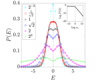
(a)

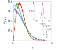
(b)

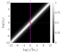
(c)