The role of orbital angular momentum constraints in the variational optimization of the two-electron reduced-density matrix
Abstract
The direct variational determination of the two-electron reduced-density matrix (2-RDM) is usually carried out under the assumption that the 2-RDM is a real-valued quantity. However, in systems that possess orbital angular momentum symmetry, the description of states with a well-defined, non-zero -projection of the orbital angular momentum requires a complex-valued 2-RDM. We consider a semidefinite program suitable for the direct optimization of a complex-valued 2-RDM and explore the role of orbital angular momentum constraints in systems that possess the relevant symmetries. For atomic systems, constraints on the expectation values of the square and -projection of the orbital angular momentum operator allow one to optimize 2-RDMs for multiple orbital angular momentum states. Similarly, in linear molecules, orbital angular momentum projection constraints enable the description of multiple electronic states, and, moreover, for states with a non-zero -projection of the orbital angular momentum, the use of complex-valued quantities is essential for a qualitatively correct description of the electronic structure. For example, in the case of molecular oxygen, we demonstrate that orbital angular momentum constraints are necessary to recover the correct energy ordering of the lowest-energy singlet and triplet states near the equilibrium geometry. However, care must still be taken in the description of the dissociation limit, as the 2-RDM-based approach is not size consistent, and the size-consistency error varies dramatically, depending on the -projections of the spin and orbital angular momenta.
I Introduction
It has long been understood that the direct variational determination of the elements of the two-electron reduced-density matrix (2-RDM) is a desirable prospect.Hus ; Löwdin (1955); May The 2-RDM affords a much more compact representation of the electronic structure than is offered by the -electron wavefunction, and, yet, it contains sufficient information to exactly specify the electronic energy for any many-electron system. Hence, the wavefunction can, in principle, be supplanted by the 2-RDM in variational calculations, provided that the space of 2-RDMs over which the optimization is performed is restricted to contain only those that derive from antisymmetrized -electron wavefunctions. Such 2-RDMs are said to be -representable.Coleman (1963) One of the strengths of 2-RDM-based methods is that they are naturally multiconfigurational and can thus be applied to multireference or strongly-correlated electronic structure problems. Indeed, variational 2-RDM (v2RDM) approachesGarrod et al. (1975); Mihailović and Rosina (1975); Rosina and Garrod (1975); Erdahl et al. (1979); Erdahl (1979); Nakata et al. (2001); Mazziotti and Erdahl (2001); Mazziotti (2002, 2006); Zhao et al. (2004); Fukuda et al. (2007); Cancès et al. (2006); Verstichel et al. (2009); Fosso-Tande et al. (2016a); Verstichel et al. (2011) that enforce necessary ensemble -representability conditionsGarrod and Percus (1964); Zhao et al. (2004); Erdahl (1978) can be used to realize a polynomially-scaling approximationGidofalvi and Mazziotti (2008); Fosso-Tande et al. (2016b) to complete active space self-consistent field (CASSCF) theoryRoos and Taylor (1980); Siegbahn et al. (1980, 1981); Roos (1987) that is applicable to active spaces composed of as many as 64 electrons in 64 orbitals.Mullinax et al. (2019)
Such nice properties notwithstanding, v2RDM approaches suffer from a number of well-known issues that limit their application to general quantum chemical problems. For example, the methods sometimes dissociate molecules into fractionally charged species.Van Aggelen et al. (2009); Verstichel et al. (2010); van Aggelen et al. (2011) The source of this error is the lack of a derivative discontinuity in the energy when considering fractionally charged atoms; the same issue arises within density functional theory.Cohen et al. (2008) Second, the direct application of the v2RDM approach to excited states is an outstanding problem. Spin-symmetry constraints give one access to multiple (lowest-energy) spin states, but, even then, one cannot reliably compare states that have the same total spin angular momentum but different -projections, as known -representability conditions do not constrain the 2-RDMs representing these states equally.van Aggelen et al. (2012). The next logical step would be the application of spatial symmetry constraints to differentiate electronic states. However, this strategy cannot be easily realized within the v2RDM framework because the point-group of the molecule is an -electron property, the evaluation of which requires knowledge of the -electron reduced-density matrix.
This work aims to at least partially address this last deficiency of the v2RDM approach. In systems possessing well-defined orbital angular momentum symmetry (i.e., atoms and linear molecules), the application of appropriate orbital angular momentum constraints allows for the direct description of multiple electronic states with different spatial symmetries. The application of v2RDM techniques to atomic states with non-zero magnitude and -projection of the orbital angular momentum requires the consideration of complex-valued reduced-density matrices (RDMs). While atomic states with non-zero magnitude and zero -projection of the orbital angular momentum can be described with real-valued RDMs, we show that the quality of the energy is inferior to that corresponding to non-zero -projection states. This behavior is reminiscent of that observed for different spin angular momentum projection states in Ref. 33. For linear molecular systems, we demonstrate that angular momentum constraints and complex RDMs can be necessary for even a qualitatively correct description of the electronic structure; for example, in a correlation-consistent polarized valence double-zeta (cc-pVDZ)Dunning (1989) basis set, a real-valued v2RDM computation incorrectly predicts that the lowest-energy state of molecular oxygen is a singlet.
This paper is organized as follows. Section II outlines the general procedure for the direct determination of the 2-RDM under ensemble -representability conditions and describes how one can incorporate orbital angular momentum constraints into the optimization. Section III then provides some of the technical details of our computations. We explore the role of orbital angular momentum constraints in atomic and linear molecular systems in Sec. IV, and some concluding remarks are provided in Sec. V.
II Theory
II.1 The variational optimization of the 2-RDM
The electronic energy of a many-electron system is a linear functional of the one-electron reduced-density matrix (1-RDM) and the 2-RDM:
| (1) |
Here, represents a two-electron repulsion integral, represents the sum of the one-electron kinetic energy and electron/nuclear potential energy integrals, and the summation indices run over all spatial orbitals. The 1-RDM and 2-RDM can be expressed in second-quantized notation as
| (2) |
and
| (3) |
respectively, where () represents a fermionic creation (annihilation) operator, and, throughout, Greek labels represent either or spin. The 1- and 2-RDM can be determined directly via the minimization of Eq. II.1 with respect to variations in their elements, provided that the optimization is constrained such that it considers only those reduced-density matrices (RDMs) that are derivable from an ensemble of antisymmetrized -electron wavefunctions. In practical computations, we can only reasonably enforce approximate -representability conditions, and the resulting energy is thus a lower-bound to the exact (full configuration interaction [CI]) energy within the relevant basis set. In this work, we consider the two-particle (“PQG”) -representability constraints of Garrod and Percus.Garrod and Percus (1964)
As we are concerned with non-relativistic Hamiltonians, we also enforce constraints on the spin structure of the 1- and 2-RDM. For example, the total spin of the system is related to an off-diagonal trace of the 2-RDM,Pérez-Romero et al. (1997); Gidofalvi and Mazziotti (2005)
| (4) |
where and represent the total spin and spin-projection quantum numbers, respectively. In addition, in all computations presented herein, the RDMs are constrained to represent maximal spin-projection states, as it has been demonstrated that such states are better described by v2RDM methods than other spin-projection states.van Aggelen et al. (2012) Maximal spin-projection states must satisfy
| (5) |
where represents a spin angular momentum raising operator. Eq. 5 implies a weaker set set of constraints of the formvan Aggelen et al. (2012)
| (6) |
which can be expressed in terms of the one-particle one-hole RDM ()
| (7) |
whose elements are given by
| (8) |
Similarly, the adjoint of the raising operator acting on the bra space also annihilates the state, giving rise to a complementary set of constraints
| (9) |
The direct variational optimization of the 1- and 2-RDM subject to the constraints outlined above constitutes a semidefinite programming (SDP) problem. We solve this problem using a modified boundary-point SDP algorithmPovh et al. (2006); Malick et al. (2009); Mazziotti (2011) similar to that described in Ref. 23. As discussed below, the introduction of orbital angular momentum constraints requires that the boundary-point algorithm be generalized to treat complex RDMs.
II.2 Orbital angular momentum constraints
Consider the Hamiltonian for an atomic many-electron system. At the non-relativistic limit, the operators corresponding to the square of the orbital angular momentum () and its projection onto the -axis () commute with this Hamiltonian. Hence, RDMs corresponding to good orbital angular momentum states should satisfy additional equality constraints, including
| (10) |
and
| (11) |
where and represent the total orbital angular momentum and orbital angular momentum projection quantum numbers, respectively. These constraints can be expressed in terms of the elements of the 1- and 2-RDM as
| (12) | |||||
and
| (13) |
where and represent matrix elements of the -component of the angular momentum operator and its square, respectively.
A 1-RDM that satisfies Eq. 13 is not guaranteed to represent a wavefunction that is an eigenfunction of . Accordingly, we also consider a constraint on the variance in , , which can be evaluated with knowledge of the 2-RDM as
| (14) | |||||
Here, we have assumed that the 1-RDM satisfies Eq. 13, and, thus, . Similar arguments could be made for RDMs that satisfy Eq. 12, so a constraint on the variance of , , might also be desirable. However, the evaluation of this quantity requires knowledge of the four-particle RDM, so this constraint will not be considered in this work.
Since the angular momentum operator is pure imaginary, the RDMs that enter our computations can only represent states with non-zero if they are allowed to take on complex values. Although the boundary-point SDP algorithm was initially defined using real matrices, its extension to the optimization of complex and even quaternion matrices is a purely technical challenge. Goemans and Williamson (2004); Wolkowicz et al. (2012) Realizing that the field of complex matrices, , is isomorphic to the field of real matrices of the form
| (15) |
one can map the complex SDP programming problem to a real one with RDMs of twice the original dimension, and, thus, a conventional SDP algorithm can be applied.
As discussed in Refs. 39 and 23, the boundary-point SDP solver for the v2RDM problem is a two-step procedure. In the first step, the dual solution to the SDP (y) is updated by solving
| (16) |
using conjugate gradient (CG) techniques. Here, x represents the primal solution vector (which maps onto the RDMs), y and z represent dual solution vectors, c represents a vector containing the one- and two-electron integrals that define the quantum system, and A and b represent the constraint matrix and vector, respectively, which encode the -representability conditions. The symbol represents a penalty parameter. In the second step, the primal solution x and the secondary dual solution z are updated via the solution of an eigenvalue problem. The rate-limiting step in this algorithm is the latter one, and its computational cost increases with the third-power of the dimension of the RDMs. As such, expanding the complex RDMs as is done in Eq. 15 will increase the number of floating-point operations required by the boundary-point SDP algorithm by a factor of eight.
We have performed numerical tests to determine the relative efficiency of real symmetric (DSYEV) and complex Hermitian (ZHEEV) eigensolvers. The wall time required to diagonalize a complex matrix of dimension 4000 is roughly 30% of that required for the diagonalization of a real symmetric matrix of twice the dimension, when using Intel’s MKL library and one core of an Intel Core i7-6850K CPU. Hence, we elect to retain the use of complex RDMs and modify the boundary-point solver accordingly. The only substantive change is that the number of coupled linear equations represented by Eq. 16 increases by a factor of two; one set of equations is used to update , while the other determines . Because the constraints we consider do not directly couple the real and imaginary components of the RDMs, these equations can be solved independently.
III Computational details
The boundary-point SDP solver for the complex v2RDM problem was implemented as a plugin to the Psi4 electronic structure package.Parrish et al. (2017) Optimized RDMs obtained from this plugin satisfied the PQG -representability conditions and the spin angular momentum constraints outlined in Sec. II. Energies from v2RDM computations were compared to those from full CI and multireference CI (MRCISD+Q) computations performed with the Psi4 and ORCA Neese (2018) packages, respectively. All orbitals were considered active within all v2RDM and full CI computations, while the reference computations for MRCISD+Q considered only full valence active spaces. All computations on atomic systems employed the cc-pVDZ basis set, while linear molecular systems were described by the STO-3GSTO , Dunning-Hay double zeta (D95V)Dun , 6-31G*,Hehre et al. (1972); Hariharan and Pople (1973); Francl et al. (1982) and cc-pVDZ basis sets; the reader is referred to Sec. IV.2 for additional details.
For atomic systems, the v2RDM procedure was considered converged when and , with the exception of two cases identified in Table 2 for which the convergence were achieved at least at and . Here, refers to the maximum of the primal error () and dual error (), and the primal/dual energy gap, , is defined as . For linear molecular systems, the v2RDM procedure was considered converged when and , with the exception of several calculations used to produce Fig. 3. The most challenging calculation could only be converged to and , and six other calculations were converged to at least and . The reader is referred to the Supporting Information for additional details.
All v2RDM computations exploited the block structure of the RDMs resulting from spin and abelian point-group symmetry considerations, but it should be noted that the point group was chosen in each case such all operators belonged to the totally symmetric irreducible representation. Hence, computations in which we constrained the expectation values of were performed within the point group, and computations in which we constrained the expectation value of were performed within the point group.
The orbital angular momentum constraints outlined in Sec. II.2 involve molecular integrals that do not usually arise in quantum chemical energy calculations. The molecular integrals over the orbital angular momentum operator, , were obtained from the standard molecular integral library in Psi4. On the other hand, the integrals over the square of the angular momentum operator are not implemented in this package. We evaluated integrals of the form numerically, where , and represents an atomic basis function. Numerical integrals were evaluated on the same quadrature grids employed with density functional theory (DFT) computations in Psi4. We use the Lebedev-Trueutler (75,302) grid, which is the default grid for all DFT computations in Psi4.
IV Results and discussion
| designation | RDM complexity | constraints enforced |
|---|---|---|
| real | real | |
| complex | complex | |
| L2 | complex | |
| Lz | complex | , |
| L | complex | , , |
In this Section, we numerically evaluate the effects of orbital angular momentum constraints in v2RDM computations on systems with well-defined orbital angular momentum symmetry. Table 1 provides the designations used to describe the constraints applied in calculations on atomic systems, as well as the complexity of the RDMs. Note that the consideration of symmetry does not require the use of complex RDMs, but L2 computations were performed using our complex-valued v2RDM algorithm nonetheless.
IV.1 Atomic systems
Figure 1 illustrates the errors in the ground-state energies of second-row atoms computed at the v2RDM level of theory, relative to energies obtained from full CI computations. First, as a technical note, the error incurred when using complex- and real-valued RDMs is nearly indistinguishable on this scale, which suggests that our complex-valued boundary-point SDP algorithm is implemented correctly. Second, we note that the error increases, in general, with the number of electrons. This observation is consistent with the fact that v2RDM methods with approximate -representability constraints are not strictly size extensive. However, in the absence of orbital angular momentum constraints, the error does not increase monotonically with system size; it is exaggerated for states with non-zero orbital angular momentum. For these states, the application of constraints results in a minor improvement. On the other hand, constraints on the expectation value of lead to a significant improvement in accuracy. Here, these non-zero angular momentum states are taken to have the maximal orbital angular momentum, which results in complex-valued RDMs. The subsequent application of variance constraints [] leads to essentially no improvement in the description of these maximal orbital angular momentum projection states.
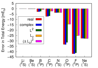
Clearly, orbital angular momentum constraints play an important role in the v2RDM-based description of ground states with non-zero total angular momentum. The data in Fig. 1 indicate that, in some cases (boron, carbon, and oxygen), the application of such constraints reduces the error in the v2RDM energy by more than a factor of two. Moreover, angular momentum constraints also allow us to directly optimize 2-RDMs for excited states that are not otherwise accessible by v2RDM methods. Table 2 illustrates energy differences between excited spin and orbital angular momentum states and the ground electronic states for all second-row atoms, except lithium and neon. Note that all results tabulated under the heading “Lz” correspond to the maximum orbital angular momentum projection. First, we consider those states that are accessible without angular momentum constraints (all cases in Table 2 for which numerical values are given under the heading “real”). For the beryllium atom, the 1S 3P transition is equally well-described by all combinations of angular momentum constraints considered. On the other hand, the description of every other transition energy is improved by the consideration of angular momentum constraints, sometimes dramatically so. In particular, the consideration of symmetry improves the almost 1 eV error in the description of the 4S 2D transition in nitrogen by 0.32 eV. The subsequent application of the constraint on reduces the error to only 0.15 eV.
Now, consider those cases in Table 2 where no numerical values are given under the heading “real;” the excited states in question are inaccessible to the v2RDM approach unless angular momentum constraints are imposed. In one case, the 4S 4P transition in nitrogen, a constraint on the expectation value of yields a terrible estimate of the excitation energy; it is too low by 5.78 eV. However, subsequent application of the constraint on yields an excitation energy that agrees with that from the full CI to within less than 0.01 eV. We also observe that the application of the constraint improves over the consideration of the constraint alone for the 4S 2P transition in nitrogen, although the improvement is less dramatic in this case. On the other hand, it appears that the application of the constraint alone gives superior results to the application of both and constraints in the cases of the 3P 1S transitions in carbon and oxygen. We believe this behavior stems from an inconsistency in the description of different and states in v2RDM methods in general. For example, for linear chains of hydrogen atoms, we have foundFosso-Tande et al. (2016a) that large- states are more well-constrained than low- states. That effect, combined with an apparent complementary effect regarding the relative description of large- and small- states, results in estimates of the absolute energies of the 1S states that are relatively poor, as compared to estimates of the absolute energies of higher angular momentum states in the same atoms (the absolute energies for all states considered here are tabulated in the Supporting Information). The application of constraints alone (i.e., without constraints on ) overstabilizes the 3P states, resulting is a fortuitous cancellation of error in the description of the 3P 1S transitions in carbon and oxygen.
| atom | transition | real | L2 | Lz | full CI | |
|---|---|---|---|---|---|---|
| Be | 1S 3P | 2.75 | 2.75 | 2.75 | 2.75 | |
| B | 2P 4P | 3.56 | 3.56 | 3.52 | 3.51 | |
| C | 3P 1D | 0.86 | 1.18 | 1.44 | 1.49 | |
| C | 3P 1S | – | 2.80 | 2.68 | 2.93 | |
| C | 3P 5S | 4.11 | 4.10 | 3.98 | 3.93 | |
| N | 4S 2D | 1.75 | 2.07 | 2.57 | 2.72 | |
| N | 4S 2P | – | 2.92 | 3.40b | 3.31 | |
| N | 4S 4P | – | 5.46 | 11.24 | 11.24 | |
| O | 3P 1D | 1.57 | 1.71 | 2.03 | 2.14 | |
| O | 3P 1S | – | 4.28 | 3.82 | 4.30 | |
| F | 2P 4P | 34.96 | 34.97 | 35.00b | 35.00 |
a For values labeled as “real,” the specification of the
spin angular momentum state is meaningful, while the specification
of the orbital angular momentum state is not.
b Loose convergence criteria were employed (Eh and ).
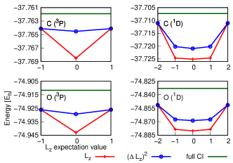
To this point, all computations enforcing constraints on considered only the maximal orbital projection state. Here, we demonstrate that, for a given -state, different orbital angular momentum projections are not treated on equal footing by the v2RDM approach. Figure 2 illustrates the energy for each state within the manifold of states associated with the 3P and 1D terms of the carbon and oxygen atoms. For comparison, the horizontal lines represent the corresponding full CI energies for each state. Clearly, the v2RDM approach fails to recover the proper degeneracy of different angular momentum projection states. Rather, the v2RDM energy is a convex function of the expectation value of , with the maximal projection states giving the best lower-bound to the full CI energy. Similar observations were made by van Aggelen et al.,van Aggelen et al. (2012) regarding the treatment of spin projection states within v2RDM theory. The consideration of constraint does not improve the quality of the v2RDM results over the case in which a real-valued algorithm is applied; this result is not too surprising, since any purely real-valued 1-RDM satisfies this constraint. What is more interesting is that forcing the variance to vanish substantially improves the quality of the non-maximal orbital angular momentum projections, most dramatically so for the state; such a constraint could be applied within a real-valued v2RDM optimization. On the other hand, variance constraints do not appear to improve the quality of the maximal orbital angular momentum projection states. Again, this behavior is similar to that observed in Ref. 33 for spin projection states. In that work, the application of pure-state and ensemble spin conditions yielded comparable results for maximal spin projection states.
IV.2 Linear molecular systems
Unlike the Hamiltonian for atomic systems, the Hamiltonian for linear molecular systems does not commute with , so, in this case, the only good orbital angular momentum quantum number is , the projection of the orbital angular momentum on the internuclear axis (which we have chosen to be aligned in the -direction). The results presented above for atomic systems suggest that orbital angular momentum projection constraints may play a similarly important role in the v2RDM-based description of states with non-zero (e.g., , , , etc. states). Hence, in this Section, we explore the utility of constraints on and in linear molecular systems, beginning with a simple question: at the v2RDM level of theory, is the ground state of molecular oxygen a singlet or a triplet?
Table 3 illustrates the energy gap between the and states of molecular oxygen, as computed at the v2RDM, full CI, and MRCISD+Q levels of theory, in various basis sets. Here, a positive value for the gap indicates that the triplet is lower in energy. Note that values labeled as “real” were generated without the consideration of orbital angular momentum constraints, so the orbital angular momentum is technically unspecified in these cases. In a minimal (STO-3G) basis, such a real-valued v2RDM computation predicts a triplet/singlet gap of 0.914 eV, which is in reasonable agreement with that from full CI (1.042 eV). However, the v2RDM result is surprisingly sensitive to the size of the basis set; in a 3-21G basis, the triplet/singlet gap reduces to 0.424 eV, and, in a cc-pVDZ basis, the singlet is actually predicted to be lower in energy than the triplet by almost 0.2 eV. Table 3 also provides results from complex-valued v2RDM computations in which we have placed constraints on the expectation value and variance of , where for the triplet state () and for the singlet state (). The application of orbital angular momentum constraints significantly improves the v2RDM results, in all basis sets. In particular, and constraints remedy the qualitative failure of the v2RDM approach within the cc-pVDZ basis. In this case, the predicted triplet/singlet gaps are 0.924 eV and 0.940 eV, respectively, which are both in reasonable agreement with the value of 1.049 eV predicted by MRCISD+Q.
| STO-3G | 3-21G | cc-pVDZ | |
|---|---|---|---|
| MRCISD+Q | 1.042b | 1.113 | 1.049 |
| real | 0.914 | 0.424 | -0.196 |
| Lz | 1.031 | 1.132 | 0.924 |
| L | 1.037 | 1.162 | 0.940 |
a For values labeled as “real,” the specification of the
spin angular momentum state is meaningful, while the specification
of the orbital angular momentum state is not.
b This value was obtained from the full CI.
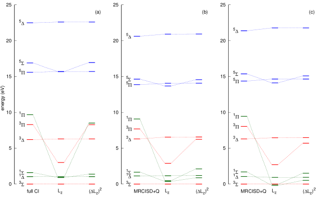
In the cc-pVDZ basis set, the imposition of orbital angular momentum constraints is clearly important for obtaining the correct ordering of the spin angular momentum states of molecular oxygen. However, these constraints cannot guarantee the correct ordering of orbital angular momentum states within a given spin manifold; this trend is evident in energy diagrams depicted in Fig. 3. In these diagrams, the energy levels in all cases are shifted such that the energy of the state is zero. In a minimal basis set [Fig. 3(a)], the full CI, v2RDM [Lz], and v2RDM [(Lz)2] approaches all predict that the is the ground state. When constraining only the expectation value of , the v2RDM approach incorrectly predicts that the three singlet states considered are nearly degenerate, and the energy of the state in particular is severely underestimated. Further, the energies of the and states are far too low. With variance constraints, the v2RDM approach recovers the correct ordering for all spin and orbital angular momentum states, but the spacing between the ground and state is still underestimated by more than 1 eV. In the D95V and cc-pVDZ basis sets [Figs. 3(b) and 3(c), respectively], we observe similar dramatic failures of the v2RDM approach (with constraints on the expectation value of ) to yield the correct state orderings, relative to the orderings obtained from MR-CISD+Q. In the cc-pVDZ basis in particular, constraints on the expectation value of alone are insufficient to yield the correct ground state; the and states are both predicted to lie below the state. Fortunately, the application of variance constraints leads to the correct prediction that the ground state of molecular oxygen is a triplet. Nonetheless, in both the D95V and cc-pVDZ basis sets, the singlet and triplet states are not ordered correctly amongst themselves; energies of the , , and states are all severely underestimated. The relative energies of all of the states considered in Fig. 3 are tabulated in the Supporting Information.
Figure 4 provides dissociation curves for the , , and states of O2, as computed at the v2RDM and MRCISD+Q levels of theory, within the D95V basis set. Here, the v2RDM curves were generated under orbital angular momentum constraints ( and ), as well as the spin angular momentum constraints outlined in Sec. II for the maximal spin projection states. As observed in Table 3, the / energy gap is well-predicted by the v2RDM approach at the equilibrium geometry, but the overall shapes of the v2RDM-derived curves are not particularly accurate. It is clear that the v2RDM approach suffers from some serious deficiencies, particularly in the limit of dissociation. The , , and curves should all share the same energy at dissociation, but they do not, regardless of the imposition of angular momentum constraints.
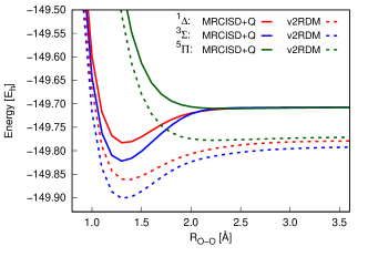
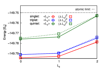
The lack of degeneracy of the , , and states in the limit of dissociation is similar to the behavior observed in Ref. 33. Those authors focused mainly on the lack of degeneracy among different states, and it is clear from that work that the maximal spin-projection states are the most well constrained, in general (i.e., these states have the highest energies). Here, we can draw similar conclusions regarding the orbital angular momentum projections. In the limit of dissociation, the ground state should have an energy equal to twice that of a single oxygen atom in its ground state (3P). Two such atoms could couple to form nine states with = 0, 1, or 2 and = 0, 1, or 2, all of which should be degenerate at large O–O bond distances. Figure 5 illustrates the energy of these nine states at an O–O bond length of 5.0 Å; in all cases, the spin-projection state is chosen to be the maximal one. The dashed line represents twice the energy of an isolated oxygen atom in the 3P state, as described by the v2RDM method (constraining the maximal spin and orbital angular momentum projection states, but not the expectation value of ). We can draw two conclusions from these data. First, for a given spin state, higher orbital angular momentum projection states are more well constrained. Second, for a given orbital angular momentum projection state, the highest-multiplicity state is the most well constrained. Indeed, the highest energy is obtained for the state; the size consistency error ( - 2 ) is only 2.9 m in this case.
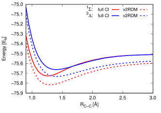
Lastly, we consider dissociation curves for the and states of another linear molecular system, C2. It is well known that a proper description of these states requires a sophisticated treatment of electron correlation effects,Abrams and Sherrill (2004); Booth et al. (2011); Mazziotti (2007) and, in the absence of orbital angular momentum constraints, v2RDM methods can only describe whichever state lies lower in energy. What is more problematic is that, because the potential energy curves for the and states should cross, a real-valued v2RDM computation may yield RDMs for different electronic states at different C–C bond lengths. Figure 6 illustrates v2RDM and full CI potential energy curves for C2 computed within the 6-31G* basis set. Full CI results were taken from Ref. 49. The application of orbital angular momentum constraints facilitates the description of both states via the v2RDM approach, and, near the equilibrium geometry for the ground state, we observe reasonable splittings between the ground and excited states. At a C–C bond length of 1.25 Å, full CI predicts that the state lies 2.43 eV above the state, while the v2RDM approach predicts that these states are separated by 2.90 eV. The relative overstabilization of the state is consistent with our observation that, for a given spin state, higher orbital angular momentum projection states are more well-constrained. Unfortunately, the v2RDM method exhibits two qualitative failures for this system. First, it predicts that the state is the ground state for all C–C bond lengths; that is, the potential energy cures for the two states are predicted to never cross. Second, as was observed above for molecular oxygen, the two electronic states considered here do not share the same dissociation limit.
V Conclusions
In systems with well-defined orbital angular momentum symmetry, the application of orbital angular momentum constraints facilitates the direct variational determination of 2-RDMs for multiple electronic states. Moreover, without such considerations, the v2RDM approach cannot qualitatively describe states with non-zero -projection of the orbital angular momentum, even if the state in question is the lowest-energy state of a given spin symmetry. Indeed, we demonstrated that, in the absence of orbital angular momentum constraints, the v2RDM approach incorrectly predicts that the ground state of molecular oxygen (described by the cc-pVDZ basis set) is a singlet. The application of appropriate constraints, which necessitates the consideration of complex-valued RDMs, recovers the correct spin-state ordering.
The v2RDM energy appears to be a convex function of the expectation value of , and, for a given magnitude of the orbital angular momentum, maximal orbital angular momentum projection states are the most well-constrained. This result reveals a qualitative failure of v2RDM methods: they do not to recover the correct degeneracy for different / states, at least when the RDMs satisfy the ensemble -representability conditions considered in this work. This behavior suggests that the conclusions of Ref. 33 regarding the description of different spin projection states apply to angular momentum projection states in general. Presumably, should one consider the direct optimization of 2-RDMs corresponding to different total angular momentum states, similarly incorrect behavior would emerge.
Acknowledgments
This work was supported as part of the Center for Actinide Science and Technology (CAST), an Energy Frontier Research Center funded by the U.S. Department of Energy, Office of Science, Basic Energy Sciences under Award No. DE-SC0016568.
References
- (1) K. Husimi, Proc. Phys. Math. Soc. Jpn. 22, 264 (1940).
- Löwdin (1955) P.-O. Löwdin, Physical Review 97, 1474 (1955).
- (3) J. E. Mayer, Phys. Rev. 100, 1579 (1955).
- Coleman (1963) A. J. Coleman, Reviews of Modern Physics 35, 668 (1963).
- Garrod et al. (1975) C. Garrod, M. V. Mihailović, and M. Rosina, Journal of Mathematical Physics 16, 868 (1975).
- Mihailović and Rosina (1975) M. Mihailović and M. Rosina, Nuclear Physics A 237, 221 (1975), ISSN 0375-9474.
- Rosina and Garrod (1975) M. Rosina and C. Garrod, Journal of Computational Physics 18, 300 (1975), ISSN 0021-9991.
- Erdahl et al. (1979) R. M. Erdahl, C. Garrod, B. Golli, and M. Rosina, Journal of Mathematical Physics 20, 1366 (1979).
- Erdahl (1979) R. Erdahl, Reports on Mathematical Physics 15, 147 (1979), ISSN 0034-4877.
- Nakata et al. (2001) M. Nakata, H. Nakatsuji, M. Ehara, M. Fukuda, K. Nakata, and K. Fujisawa, J. Chem. Phys. 114, 8282 (2001).
- Mazziotti and Erdahl (2001) D. A. Mazziotti and R. M. Erdahl, Phys. Rev. A 63, 042113 (2001).
- Mazziotti (2002) D. A. Mazziotti, Phys. Rev. A 65, 062511 (2002).
- Mazziotti (2006) D. A. Mazziotti, Phys. Rev. A 74, 032501 (2006).
- Zhao et al. (2004) Z. Zhao, B. J. Braams, M. Fukuda, M. L. Overton, and J. K. Percus, J. Chem. Phys. 120, 2095 (2004).
- Fukuda et al. (2007) M. Fukuda, B. J. Braams, M. Nakata, M. L. Overton, J. K. Percus, M. Yamashita, and Z. Zhao, Mathematical Programming 109, 553 (2007), ISSN 0025-5610.
- Cancès et al. (2006) E. Cancès, G. Stoltz, and M. Lewin, J. Chem. Phys. 125, 064101 (2006).
- Verstichel et al. (2009) B. Verstichel, H. van Aggelen, D. Van Neck, P. W. Ayers, and P. Bultinck, Phys. Rev. A 80, 032508 (2009).
- Fosso-Tande et al. (2016a) J. Fosso-Tande, D. R. Nascimento, and A. E. D. III, Molecular Physics 114, 423 (2016a).
- Verstichel et al. (2011) B. Verstichel, H. van Aggelen, D. V. Neck, P. Bultinck, and S. D. Baerdemacker, Computer Physics Communications 182, 1235 (2011), ISSN 0010-4655.
- Garrod and Percus (1964) C. Garrod and J. K. Percus, Journal of Mathematical Physics 5, 1756 (1964).
- Erdahl (1978) R. M. Erdahl, Int. J. Quantum Chem. 13, 697 (1978), ISSN 1097-461X.
- Gidofalvi and Mazziotti (2008) G. Gidofalvi and D. A. Mazziotti, J. Chem. Phys. 129, 134108 (2008).
- Fosso-Tande et al. (2016b) J. Fosso-Tande, T.-S. Nguyen, G. Gidofalvi, and A. E. DePrince, Journal of Chemical Theory and Computation 12, 2260 (2016b), pMID: 27065086.
- Roos and Taylor (1980) B. O. Roos and P. R. Taylor, Chem. Phys. 48, 157 (1980).
- Siegbahn et al. (1980) P. Siegbahn, A. Heiberg, B. Roos, and B. Levy, Phys. Scripta 21, 323 (1980).
- Siegbahn et al. (1981) P. E. M. Siegbahn, J. Almlöf, A. Heiberg, and B. O. Roos, J. Chem. Phys. 74, 2384 (1981).
- Roos (1987) B. O. Roos, Advances in Chemical Physics; Ab Initio Methods in Quantum Chemistry Part 2 (John Wiley and Sons, Ltd., 1987), vol. 69, pp. 399–445.
- Mullinax et al. (2019) J. W. Mullinax, L. Koulias, E. Maradzike, E. Epifanovsky, G. Gidofalvi, and A. E. DePrince, XXX XXX, submitted (2019).
- Van Aggelen et al. (2009) H. Van Aggelen, P. Bultinck, B. Verstichel, D. Van Neck, and P. W. Ayers, Phys. Chem. Chem. Phys. 11, 5558 (2009).
- Verstichel et al. (2010) B. Verstichel, H. van Aggelen, D. Van Neck, P. W. Ayers, and P. Bultinck, J. Chem. Phys. 132, 114113 (2010).
- van Aggelen et al. (2011) H. van Aggelen, B. Verstichel, P. Bultinck, D. V. Neck, P. W. Ayers, and D. L. Cooper, J. Chem. Phys. 134, 054115 (2011).
- Cohen et al. (2008) A. J. Cohen, P. Mori-Sánchez, and W. Yang, Science 321, 792 (2008).
- van Aggelen et al. (2012) H. van Aggelen, B. Verstichel, P. Bultinck, D. V. Neck, and P. W. Ayers., J. Chem. Phys. 136, 014110 (2012).
- Dunning (1989) T. H. Dunning, J. Chem. Phys. 90, 1007 (1989).
- Pérez-Romero et al. (1997) E. Pérez-Romero, L. M. Tel, and C. Valdemoro, Int. J. Quantum Chem. 61, 55 (1997).
- Gidofalvi and Mazziotti (2005) G. Gidofalvi and D. A. Mazziotti, Phys. Rev. A 72, 052505 (2005).
- Povh et al. (2006) J. Povh, F. Rendl, and A. Wiegele, Computing 78, 277 (2006), ISSN 1436-5057.
- Malick et al. (2009) J. Malick, J. Povh, F. Rendl, and A. Wiegele, SIAM Journal on Optimization 20, 336 (2009).
- Mazziotti (2011) D. A. Mazziotti, Phys. Rev. Lett. 106, 083001 (2011).
- Goemans and Williamson (2004) M. X. Goemans and D. P. Williamson, Journal of Computer and System Sciences 68, 442 (2004), ISSN 0022-0000, special Issue on STOC 2001.
- Wolkowicz et al. (2012) H. Wolkowicz, R. Saigal, and L. Vandenberghe, Handbook of Semidefinite Programming: Theory, Algorithms, and Applications, International Series in Operations Research & Management Science (Springer US, 2012), ISBN 9781461543817.
- Parrish et al. (2017) R. M. Parrish, L. A. Burns, D. G. A. Smith, A. C. Simmonett, A. E. DePrince, E. G. Hohenstein, U. Bozkaya, A. Y. Sokolov, R. Di Remigio, R. M. Richard, et al., J. Chem. Theory Comput. (2017).
- Neese (2018) F. Neese, Wiley Interdisciplinary Reviews: Computational Molecular Science 8, e1327 (2018).
- (44) W.J. Hehre, R.F. Stewart and J.A. Pople, J. Chem. Phys. 2657 (1969).
- (45) T. H. Dunning Jr. and P. J. Hay, in Modern Theoretical Chemistry, Ed. H. F. Schaefer III, Vol. 3 (Plenum, New York, 1977) 1-28.
- Hehre et al. (1972) W. J. Hehre, R. Ditchfield, and J. A. Pople, J. Chem. Phys. 56, 2257 (1972), URL https://doi.org/10.1063/1.1677527.
- Hariharan and Pople (1973) P. C. Hariharan and J. A. Pople, Theoretica chimica acta 28, 213 (1973), ISSN 1432-2234, URL https://doi.org/10.1007/BF00533485.
- Francl et al. (1982) M. M. Francl, W. J. Pietro, W. J. Hehre, J. S. Binkley, M. S. Gordon, D. J. DeFrees, and J. A. Pople, J. Chem. Phys. 77, 3654 (1982), URL https://doi.org/10.1063/1.444267.
- Abrams and Sherrill (2004) M. L. Abrams and C. D. Sherrill, The Journal of Chemical Physics 121, 9211 (2004).
- Booth et al. (2011) G. H. Booth, D. Cleland, A. J. W. Thom, and A. Alavi, The Journal of Chemical Physics 135, 084104 (2011).
- Mazziotti (2007) D. A. Mazziotti, Phys. Rev. A 76, 052502 (2007).