Exploiting Nested Task-Parallelism in
the $\mathcal{H}$-LU Factorization

Abstract

We address the parallelization of the LU factorization of hierarchical matrices ($\mathcal{H}$-matrices) arising from boundary element methods. Our approach exploits task-parallelism via the OmpSs programming model and runtime, which discovers the data-flow parallelism intrinsic to the operation at execution time, via the analysis of data dependencies based on the memory addresses of the tasks’ operands. This is especially challenging for $\mathcal{H}$-matrices, as the structures containing the data vary in dimension during the execution. We tackle this issue by decoupling the data structure from that used to detect dependencies. Furthermore, we leverage the support for weak operands and early release of dependencies, recently introduced in OmpSs-2, to accelerate the execution of parallel codes with nested task-parallelism and fine-grain tasks.

1 Introduction

Hierarchical matrices (or $\mathcal{H}$-matrices) [1] provide a useful mathematical abstraction to tackle problems arising in boundary element methods, elliptic partial differential operators, and related integral equations, among others [2]. Concretely, for many of these applications, $\mathcal{H}$-matrices and the associated $\mathcal{H}$-arithmetic methods offer efficient numerical tools to store an $n\times n$ matrix using only $O(n\,k\,\log n)$ elements and compute matrix factorizations with a cost of $O(n\,k^{2}\,\log^{2}n)$ floating-point operations (flops). In these cost expressions, $k$ denotes the local rank for subblocks of the matrix, which can be tuned to trade off accuracy of the approximation for storage and computational costs [3].

The development of linear algebra methods for $\mathcal{H}$-matrices has been an active area of research during the past two decades, having produced a wide number of packages such as HLib, H2Lib and HLibPro as well as a collection of individual routines. Part of this software directly relies on the kernels from the Basic Linear Algebra Subprograms (BLAS) [4] to compute fundamental dense linear algebra (LA) operations. As a result, when linked with a multi-threaded instance of the BLAS, these $\mathcal{H}$-LA routines can seamlessly run in parallel on current multicore processors. However, this solution can extract a limited amount parallelism, bounded to that present in the individual BLAS kernels. Furthermore, for $\mathcal{H}$-matrices arising from real applications, low-rank blocks “dominate” the data structure. While this confers $\mathcal{H}$-matrices/methods their appealing low storage and computational costs, unfortunately, it also limits further the parallelism that can be extracted from individual kernels. In particular, $\mathcal{H}$-arithmetic involves memory-bounded kernels which, in general, do not benefit from a multi-threaded execution. The bottom-line is that, for practical $\mathcal{H}$-applications, it becomes necessary to exploit parallelism at a higher level.

In the last years, exploiting task-parallelism has been exposed as an appealing coarse-grain approach for the solution of dense and sparse linear systems on multi-threaded architectures [5, 6, 7, 8, 9]. These approaches discover task parallelism dynamically (at execution time) via a runtime but rely on a sequential implementation of the numerical kernels (in the dense case, BLAS) to execute the individual operations. Although similar, the factorization of $\mathcal{H}$-matrices for linear systems presents some specific challenges when the aim is to extract task-parallelism. First, the “recursive nature” of $\mathcal{H}$-matrices makes the detection and efficient exploitation of nested task-parallelism a complex endeavor. Second, handling low-rank matrices requires specialized data structures that can vary (grow/shrink in size), at execution time, with low overhead. This is particularly important given the low cost of $\mathcal{H}$-arithmetic algorithms.

In [10], we presented two prototype task-parallel versions of the $\mathcal{H}$-LU factorization using the OpenMP and OmpSs programming models [11, 12]. Our initial implementations presented several drawbacks, that we overcome in this work, making the following specific contributions:

• The prototype implementations in [10] assumed that the blocks of the $\mathcal{H}$-matrix were either dense or null. No specialized data structures and $\mathcal{H}$-arithmetic for low-rank blocks were therefore involved in the factorization. In comparison, in the present work we parallelize the $\mathcal{H}$-LU factorization as implemented in the sequential version of H2Lib, with problems involving low-rank blocks and, therefore, low-rank storage and real $\mathcal{H}$-arithmetic.

• An additional consequence of targeting the $\mathcal{H}$-LU factorization in H2Lib is the need to accommodate low-rank data structures that can change their dimensions at execution time. This is particularly challenging for a runtime-based parallelization because task dependencies are detected via an analysis of the memory addresses of the tasks’ operands. To address this problem, we propose the use of an auxiliary “skeleton” array, which reflects the block hierarchy of the $\mathcal{H}$-matrix, and can be leveraged to identify task dependencies. This additional data structure is built before the execution commences, at low cost, and remains unchanged during the complete execution, independently of the modifications on the structures containing the actual data due to the use of $\mathcal{H}$-arithmetic.

• The task-parallel implementation developed in our past work [10], based on OmpSs, forced us to operate on fine-granularity tasks with operands that were stored in contiguous regions of memory. The practical consequence of this constraint is that it was not possible to exploit the nested task-parallelism intrinsic to the $\mathcal{H}$-LU factorization. In the present work, we address these problems using the new OmpSs-2 model, with explicit support for weak dependencies and early release to take advantage of fine-grained nested parallelism [13].

The rest of the paper is structured as follows. In Sections 2 and 3, we briefly review the structure of $\mathcal{H}$-matrices in H2Lib and introduce a high-level algorithm for the LU factorization of an $\mathcal{H}$-matrix, respectively. (A complete review of $\mathcal{H}$-matrices and $\mathcal{H}$-arithmetic can be found, for example, in [1, 3].) In Section 4 we re-visit the parallelization of the $\mathcal{H}$-LU factorization in [10], exposing the limitations of those prototype codes. In Section 5 we describe the new task-level parallelization of the hierarchical factorization, offering details on the use of the skeleton structure to detect task dependencies and the exploitation of fine-grained nested parallelism via weak dependencies. Finally, in Section 6 we provide a complete experimental evaluation of the task-parallel codes, and in Section 7 we close the paper with a few concluding remarks.

2 Representation of $\mathcal{H}$-Matrices in H2Lib

In this section we briefly introduce the structure of $\mathcal{H}$-matrices and how they are implemented in H2Lib. This sequential library, written in C, offers a state-of-the-art implementation of $\mathcal{H}$-matrix techniques, including sophisticated data structures, support for $\mathcal{H}$-arithmetic operations such as multiplication, inversion and factorization, compression schemes for non-local operators, and fast re-compression algorithms.

The main idea behind $\mathcal{H}$-matrices relies on finding a partition over a matrix into blocks which are either small in dimension or admissible in the sense that they can be stored efficiently using low-rank data structures instead of dense ones. Utilizing low-rank matrices is a prerequisite for reducing the storage and computational costs down to log-linear functions on the number of elements and flops, respectively.

Before we can find a partition of the matrix into a set of subblocks, we need to “organize” the degrees of freedom (DoFs) into sets, which can be handled efficiently via a tree-like structure called clustertree. Therefore, we assume that we know the geometric extent of every degree of freedom that appears in our application. This frequently reduces to the support of finite element basis functions. Armed with that information, we can setup an axis-parallel bounding box $\mathcal{B}_{t}$, which contains the union of all extents corresponding to the cluster $t$. This box will now be splitted into two parts along some geometrical dimension, which yields two independent boxes $\mathcal{B}_{t_{1}},\,\mathcal{B}_{t_{2}}$. From there, we can sort each and every DoF into one of these boxes according to their position in space. Next we process both boxes recursively until the number of DoFs located in a box falls below a prescribed constant, which we denote by leafsize ($C_{lf}$). In order to handle all these boxes efficiently, we organize these clusters into a tree structure expressed by $\operatorname{sons}(t)=\{t_{1},t_{2}\}$. This procedure is summarized in Algorithm 1.

Algorithm 1 Clustertree construction

Geometric information about the degrees of freedom is stored within an array dofs of length size.

A hierarchical partition of the DoFs is returned via the clustertree t.

procedure setup_clustertree(dofs, size)

     if size $>C_{lf}$ then

         $d\leftarrow$ find_splitting_dimension(dofs, size)

         sons $\leftarrow$ 2

         $t\leftarrow$ new_cluster(dofs, size, sons)

         $\{\text{dofs1, dofs2, size1, size2}\}\leftarrow$ sort_dofs(dofs, size, $d$)

         $t_{1}\leftarrow$ setup_clustertree(dofs1, size1)

         $t_{2}\leftarrow$ setup_clustertree(dofs2, size2)

         $\operatorname{sons}(t)\leftarrow\{t_{1},t_{2}\}$

     else

         $t\leftarrow$ new_leaf_cluster(dofs, size)

     end if

     return $t$

end procedure

This hierarchical structure is realized with the following C data structure cluster within H2Lib:

⬇

1struct cluster {

2 uint size;

3 uint *dofs

4 uint *bbox_min;

5 uint *bbox_max;

6 cluster *son;

7 uint sons;

8}

Here size is the number of elements associated with this cluster and dofs is an array referring to the degrees of freedom. The bounding box $\mathcal{B}_{t}$ for a cluster $t$ is stored within the arrays bbox_min and bbox_max, respectively. In addition, son and sons represent the tree structure of the clusters.

In order to identify subblocks of the matrix, which can be approximated by a low rank representation, we need some admissibility condition, which ensures that we can find an approximation to some prescribed accuracy. For many cases, particularly for tensor-interpolation, the condition

$$\operatorname{min}\{\operatorname{diam}(t),\operatorname{diam}(s)\}\leq\operatorname{dist}(t,s)$$

guarantees this. Here diam and dist denote the Euclidean diameter of some cluster and the Euclidean distance between two clusters, respectively.

During the setup of the $\mathcal{H}$-matrix, the partitioning is performed recursively as stated in Algorithm 2, returning a tree-like block structure. For a detailed construction of such block partition, see [1, 3].

Algorithm 2 Blocktree construction

row cluster t, column cluster s.

A blocktree b is returned for the pair (t,s).

procedure setup_blocktree(t, s)

     if  admissible(t, s)  then

         b $\leftarrow$ new_admissible_block(t, s)

     else

         if  sons(t) $\neq\emptyset~{}\land$ sons(s) $\neq\emptyset$  then

              b $\leftarrow$ new_partitioned_block (t, s)

              for all t’ $\in$ sons(t), s’ $\in$ sons(s) do

                  b[t’][s’] $\leftarrow$ setup_blocktree(t’, s’)

              end for

              return b

         else

              b $\leftarrow$ new_inadmissible_block(t, s)

         end if

     end if

     return b

end procedure

In agreement with the three cases occurring in Algorithm 2, the application of Algorithm 2, at a given level of the recursion, can produce either a low-rank block (i.e., a new admissible block), a new recursive partitioning (via the same algorithm), or a conventional dense (inadmissible) block. To handle these cases, the C data type representing a $\mathcal{H}$-matrix in the H2Lib follows this structure:

⬇

1struct hmatrix {

2 cluster rc, cc;

3 rkmatrix r;

4 amatrix f;

5 hmatrix *son;

6 uint rsons, csons;

7}

In this data type, rc and cc respectively correspond to the row cluster and column cluster of he current matrix block. Low-rank matrices are stored in the structure rkmatrix, whereas dense matrices are stored in amatrix. Partitioned matrices are accommodated using an array pointing to the sons. The structure also provides the amount of sons per row and column, stored in rsons and csons, respectively.

3 LU Factorization of $\mathcal{H}$-Matrices

3.1 Algorithm for the $\mathcal{H}$-LU factorization

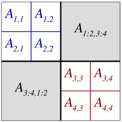
We open this section with a brief review of the algorithm for the $\mathcal{H}$-LU factorization. For this purpose, consider a sample $\mathcal{H}$-matrix $A\in\mathbb{R}^{n\times n}$, partitioned as shown in Figure 1. The factorization procedure can be formulated as a generalization of the blocked right-looking (RL) algorithm for the LU factorization [14] that exploits the hierarchical structure of the matrix.

Figure 1: $2\times 2$ partitioning of a simple $\mathcal{H}$-matrix.

In particular, the following sequence of operations computes the $\mathcal{H}$-LU factorization of $A$:

$$\begin{array}[]{l}\hline\cr\mbox{\rm Sequence of operations for the $\mathcal{H}$-LU factorization of $A$:}\\ \hline\cr\begin{array}[]{llcl}\hbox{\pagecolor{white}\parbox{17.22217pt}{{\color[rgb]{0,0,0.60}\definecolor[named]{pgfstrokecolor}{rgb}{0,0,0.60}\small{\sf\small O1.1}}}}:&A_{1,1}&=&L_{1,1}U_{1,1}\\ \hbox{\pagecolor{white}\parbox{17.22217pt}{{\color[rgb]{0,0,0.60}\definecolor[named]{pgfstrokecolor}{rgb}{0,0,0.60}\small{\sf\small O1.2}}}}:&U_{1,2}&:=&L_{1,1}^{-1}A_{1,2}\\ \hbox{\pagecolor{white}\parbox{17.22217pt}{{\color[rgb]{0,0,0.60}\definecolor[named]{pgfstrokecolor}{rgb}{0,0,0.60}\small{\sf\small O1.3}}}}:&L_{2,1}&:=&A_{2,1}U_{1,1}^{-1}\\ \hbox{\pagecolor{white}\parbox{17.22217pt}{{\color[rgb]{0,0,0.60}\definecolor[named]{pgfstrokecolor}{rgb}{0,0,0.60}\small{\sf\small O1.4}}}}:&A_{2,2}&:=&A_{2,2}-L_{2,1}\cdot U_{1,2}\\ \hbox{\pagecolor{white}\parbox{17.22217pt}{{\color[rgb]{0,0,0.60}\definecolor[named]{pgfstrokecolor}{rgb}{0,0,0.60}\small{\sf\small O1.5}}}}:&A_{2,2}&=&L_{2,2}U_{2,2}\\ \hline\cr\hbox{\pagecolor{grey}\parbox{17.22217pt}{{\color[rgb]{0,0,0}\definecolor[named]{pgfstrokecolor}{rgb}{0,0,0}\pgfsys@color@gray@stroke{0}\pgfsys@color@gray@fill{0}\small{\sf\small O2}}}}:&U_{1:2,3:4}&:=&L_{1:2,1:2}^{-1}A_{1:2,3:4}\\ \hline\cr\hbox{\pagecolor{grey}\parbox{17.22217pt}{{\color[rgb]{0,0,0}\definecolor[named]{pgfstrokecolor}{rgb}{0,0,0}\pgfsys@color@gray@stroke{0}\pgfsys@color@gray@fill{0}\small{\sf\small O3}}}}:&L_{3:4,1:2}&:=&A_{3:4,1:2}U_{1:2,1:2}^{-1}\\ \hline\cr\hbox{\pagecolor{grey}\parbox{17.22217pt}{{\color[rgb]{0,0,0}\definecolor[named]{pgfstrokecolor}{rgb}{0,0,0}\pgfsys@color@gray@stroke{0}\pgfsys@color@gray@fill{0}\small{\sf\small O4}}}}:&A_{3:4,3:4}&:=&A_{3:4,3:4}-L_{3:4,1:2}\cdot U_{1:2,3:4}\\ \hline\cr\hbox{\pagecolor{white}\parbox{17.22217pt}{{\color[rgb]{0.60,0,0}\definecolor[named]{pgfstrokecolor}{rgb}{0.60,0,0}\small{\sf\small O5.1}}}}:&A_{3,3}&=&L_{3,3}U_{3,3}\\ \hbox{\pagecolor{white}\parbox{17.22217pt}{{\color[rgb]{0.60,0,0}\definecolor[named]{pgfstrokecolor}{rgb}{0.60,0,0}\small{\sf\small O5.2}}}}:&U_{3,4}&:=&L_{3,3}^{-1}A_{3,4}\\ \hbox{\pagecolor{white}\parbox{17.22217pt}{{\color[rgb]{0.60,0,0}\definecolor[named]{pgfstrokecolor}{rgb}{0.60,0,0}\small{\sf\small O5.3}}}}:&L_{4,3}&:=&A_{4,3}U_{3,3}^{-1}\\ \hbox{\pagecolor{white}\parbox{17.22217pt}{{\color[rgb]{0.60,0,0}\definecolor[named]{pgfstrokecolor}{rgb}{0.60,0,0}\small{\sf\small O5.4}}}}:&A_{4,4}&:=&A_{4,4}-L_{4,3}\cdot U_{3,4}\\ \hbox{\pagecolor{white}\parbox{17.22217pt}{{\color[rgb]{0.60,0,0}\definecolor[named]{pgfstrokecolor}{rgb}{0.60,0,0}\small{\sf\small O5.5}}}}:&A_{4,4}&=&L_{4,4}U_{4,4}\\ \hline\cr\end{array}\end{array}$$

Dense blocks

Assuming all blocks are dense, these operations correspond to three basic linear algebra building blocks (or computational kernels):

• LU factorization (e.g., O1.1, O1.5 and O5.1);

• triangular system solve (e.g., with unit lower triangular factor in O1.2 and O2; or upper triangular factor in O1.3 and O3); and

• matrix-matrix multiplication (O1.4, O4, etc.).

In the dense case, the triangular factors $L$ and $U$ overwrite the corresponding entries of $A$ so that, for example, in O2, the output $U_{1:2,3:4}$ overwrites the input $A_{1:2,3:4}$. Furthermore, the diagonal of the unit triangular matrix $L$ only contains ones and it is not explicitly stored.

Low-rank blocks

In the $\mathcal{H}$-LU factorization, if any of the matrix blocks is represented in low-rank factorized form, the storage will have to be specialized (see section 2) and the operations involving this block will need to be performed in $\mathcal{H}$-arithmetic.

In typical $\mathcal{H}$-matrix implementations, low-rank matrices are represented in the factorized form $X=AB^{*}$, where $A$ and $B$ have only $k$ columns, so the rank of $X$ is bounded by $k$. In practice, $k$ is significantly smaller than the dimensions of the original matrix $X$.

The H2Lib packages use the following data type to store low-rank matrices:

⬇

1 typedef struct rkmatrix {

2 uint k; /* Maximal rank */

3 amatrix A; /* Left factor A */

4 amatrix B; /* Right factor B */

5 }

Basic operations for low-rank matrices $X\in\mathbb{R}^{n\times m}$ include:

• matrix-vector multiplication $y:=Xz$, performed using $y:=Xz=A(B^{*}z)$;

• multiplication of $X$ by an arbitrary matrix $Z\in\mathbb{R}^{\ell\times n}$, using $Y:=ZX=(ZA)B^{*}$,

• triangular system solve $LY=X$ or $YL=X$; by applying forward or backward substitution to the $k$ columns of $A$ or the $k$ rows of $B$, respectively.

Adding two low-rank matrices poses a challenge, since the sum of two matrices $X_{1}=A_{1}B_{1}^{*}$ and $X_{2}=A_{2}B_{2}^{*}$, of ranks $k_{1}$ and $k_{2}$, may have a rank of $k_{1}+k_{2}$. Fortunately, in typical applications a low-rank approximation can be constructed by computing, e.g., a singular value decomposition of

$$X_{1}+X_{2}=A_{1}B_{1}^{*}+A_{2}B_{2}^{*}=\begin{pmatrix}A_{1}&A_{2}\end{pmatrix}\begin{pmatrix}B_{1}&B_{2}\end{pmatrix}^{*}$$

and discarding small singular values. The same approach can be employed to convert an arbitrary matrix into a factorized low-rank matrix.

From the point of view of peak floating-point performance, working with factorized low-rank matrices poses a challenge. Concretely, while the multiplication of two $n\times n$-matrices requires $2n^{3}$ operations, i.e., $n$ operations for each coefficient transferred from main memory, only $2kn^{2}$ operations are required if one of the factors is a factorized low-rank matrix, i.e., only $k$ operations for each coefficient. Therefore we have to deal with the fact that the speed of operations involving low-rank matrices and, in consequence, $\mathcal{H}$-matrices, is generally limited by the memory bandwidth, instead of by the floating-point throughput.

3.2 Nested dependencies in the factorization

Figure 2 provides a graphical representation of the dependencies among the operations in the $\mathcal{H}$-LU factorization of the sample matrix $A$, exposing the recursion implicit in the operation. Concretely, the factorization can be initially decomposed into 5 tasks: O1, O2, O3, O4 and O5, with the dependencies among them displayed in the figure. The first and last (macro-)tasks, O1 and O5, corresponding to the factorizations of the diagonal blocks of $A$, can themselves be decomposed into 5 (sub-)tasks each, and reproduce the same dependency pattern as that of the initial factorization.

Figure 2: Data dependencies in the blocked RL algorithm for the $\mathcal{H}$-LU factorization.

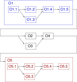
We close this section by noting that the presence of low-rank blocks does not affect the dependencies, only the particular implementation of the internal operations. Also, the sample matrix employed in this section was specifically chosen to be simple yet useful enough to expose the existence of nested parallelism in the $\mathcal{H}$-LU factorization (and discuss how to tackle it in the following sections). The dependency graph in Figure 2 seems to show that there is little task-parallelism to be exploited as, for this particular example, we can only run in parallel O1.2 with O1.3; O2 with O3; and O5.2 with O5.3. However, this is a direct consequence of the simplicity of the selected example. In contrast, an $\mathcal{H}$-matrix/block with a division (partitioning) into $b\times b$ subblocks yields a rapid explosion of the degree of task-level parallelism that is cubic in $b$, featuring a richer set of dependencies.

4 Leveraging Task-Parallelism in OmpSs

Section 3 and Figure 2 expose the recursive character of the $\mathcal{H}$-LU factorization and the presence of nested task-parallelism. In particular, coming back to our sample $\mathcal{H}$-LU factorization in the previous section, a natural approach to exploit nested task-parallelism is to annotate O1, O2, O3, O4, O5 each as a task using the OpenMP/OmpSs task construct [11, 12]. Inside O1, we can then annotate O1.1, O1.2,…,O1.5 each as a task; and a similar argument applies to the decomposition of O5 into O5.1, O5.2,…,O5.5.

This section briefly reviews the drawbacks of our prototype task-parallel $\mathcal{H}$-LU implementation in [10] due to the limited support for nested task-parallelism and hierarchical data structures in OpenMP (version 4.5) and OmpSs (version 16.06).

4.1 Using representants

The OpenMP and OmpSs runtimes identify task dependencies, at runtime, via the analysis of the memory addresses of the task operands (variables) and their directionality. In order to specify the dependencies between tasks, in dense linear algebra operations we can often use a “representant” for each task operand, which is then passed to the runtime system in order to detect these dependencies [7]. (This representant is the memory address of the matrix block computed by the corresponding operation; that is, the top-left entry of the output matrix block.) We next discuss the problem with this approach in the context of hierarchical matrices.

Let us consider, for example, the dependency O1.1$\rightarrow$O1.2, between the LU factorization

$$\begin{array}[]{rrclrlr}\mbox{{\sf\small O1.1}}:&A_{1,1}&=&L_{1,1}U_{1,1},\end{array}$$

and the triangular system solve

$$\begin{array}[]{rrclrlr}\mbox{{\sf\small O1.2}}:&U_{1,2}&:=&L_{1,1}^{-1}A_{1,2};\end{array}$$

and the dependency O1$\rightarrow$O2, between the LU factorization

$$\begin{array}[]{rrclrlr}\mbox{{\sf\small O1}}:&A_{1:2,1:2}&=&L_{1:2,1:2}U_{1:2,1:2},\end{array}$$

and the triangular system solve

$$\begin{array}[]{rrclrlr}\mbox{{\sf\small O2}}:&U_{1:2,3:4}&:=&L_{1:2,1:2}^{-1}A_{1:2,3:4}.\end{array}$$

(We note here that the composition of the operations O1.1–O1.5 yields the LU factorization of $A_{1:2,1:2}$ specified in O1.)

For simplicity, let us assume that all the blocks involved in these operations are dense. (The analysis of the dependencies for low-rank blocks is analogous.) The problem with the use of representants is that it is not possible to distinguish a dependency with input $A_{1:2,1:2}$ from one that has its origin in the input $A_{1,1}$. In particular, since both $A_{1:2,1:2}$ and $A_{1,1}$ share the same representant, with this technique it is not possible to know whether O1.2 and O2 depend either on O1.1 or O1.

4.2 Leveraging regions

OmpSs offers flexibility to specify the shapes/dimensions of the input/output operands passed to a task as regions, which can then be used to detect dependencies between the tasks. In principle, it might seem that this mechanism could be leveraged to avoid the ambiguity due to the use of representants. However, the following discussion illustrates that this is still insufficient for H2Lib.

To expose the problem, consider again the dependencies O1.1$\rightarrow$O1.2 and O1$\rightarrow$O2 where, for simplicity, we still assume that all blocks involved in these operations are dense. To tackle this case, it might seem that we could simply specify the dimensions of the operands. For example, in OmpSs, the lower triangular system solves O1.2 and O2 could be annotated as

⬇

1#pragma omp task in( L[0;M*M] ), inout( B[0;M*P] )

2void task_ltrsm( int M, int P, double *L, int LDL,

3 double *B, int LDB )

where L is (the memory address of) the M$\times$M lower triangular factor and B is (the memory address of) the M$\times$P right-hand side.

The problem with this solution is that, in H2Lib, the entries of a (dense) block which is further partitioned into subblocks (as is the case for $A_{1:2,1:2}$) are not stored contiguously in memory. Therefore, the use of a region to specify the memory address of the contents of such block is useless. The same problem appears for partitioned low-rank blocks.

Our workaround to this problem in [10] was to divide the triangular system solve in O2 into four tasks, each updating one of the four blocks of $U_{1:2,3:4}$. Unfortunately, this solution implies the need to explicitly decompose all tasks in the $\mathcal{H}$-LU factorization to operate with blocks of the “base” granularity, so that a region only spans data which is contiguous in memory. The practical consequence is that, with that approach, it was not truly possible to exploit nested task-parallelism. Furthermore, in case of small leaf blocks, the overhead introduced by the dependency-detection mechanism can be considerable, reducing the performance of the solution.

5 Extended Support for Nested Task-Parallelism in OmpSs-2

5.1 Dealing with non-contiguous regions

The (end of the) previous section identified a major problem when tackling nested parallelism and hierarchical data structures which do not lie contiguously in memory. This issue is difficult to address, as it is rooted on the hierarchical nature of the problem and the use of $\mathcal{H}$-arithmetic, which derives in the need to embody a data structure that can vary at runtime. With these premises, it becomes necessary to maintain a tree-like structure of the matrix contents (see Section 3), where only the “leaf” blocks (either dense or low-rank) store their data contiguously in memory. As a result, we cannot leverage this data structure to specify dependencies between tasks involving non-leaf blocks.

Our solution to this problem is application-specific (but can be leveraged in scenarios involving dynamic and/or complex data structures [8]) and consists of an auxiliary skeleton data structure that reflects the block structure of the $\mathcal{H}$-matrix. In particular, this data structure can be realized using an array with one representant per leaf (i.e., non-partitioned) block in the original matrix, where the representants that pertain to the same block appear in contiguous positions of memory. For the particular simple example in Figure 1 this means that, in order to detect dependencies, we use an additional array with representants for

$$A_{1,1} A_{1,2} A_{2,1} A_{2,2} A_{3:4,1:2} A_{1:2,3:4} A_{3,3} A_{3,4} A_{4,3} A_{4,4}$$

appearing in that specific order. Operating in this manner, we decouple the mechanism to detect the dependencies (based on the previous array) from the actual layout of the data in memory, which can vary during the execution.

With this solution, the ambiguity between O1.1 and O1 when dealing with the dependencies O1.1$\rightarrow$O1.2 and O1$\rightarrow$O2 is easily tackled. Concretely, although both operands share the same base address in memory (that of $A_{1,1}$ in the skeleton array), the region for O1.1 comprises a single representant while that of O1 comprises four representants in the skeleton array. We emphasize that these representants are stored contiguously in memory and this skeleton data structure does not vary during the execution (in contrast with the structure storing the actual data). Therefore, it can be built before the operations commence, and the cost of assembling it can be amortized over enough computation.

5.2 Weak dependencies and early release

The tasking model of OpenMP 4.5 supports both nesting and the definition of dependences between sibling tasks. Many operations with $\mathcal{H}$-matrices are recursive, so the natural strategy to parallelize them is to leverage task nesting. However, this top-down approach has some drawbacks since combining nesting with dependencies usually requires additional measures to enforce the correct coordination of dependencies across nesting levels. For instance, most non-leaf tasks need to include a taskwait construct at the end of their code. While these measures enforce the correct order of execution, as a side effect, they also constrain both the generation and discovery of task parallelism. In this paper we leverage the enhanced tasking model recently implemented in OmpSs-2 [13] to exploit both nesting and fine-grained data-flow parallelism.

The OmpSs-2 tasking model introduces two major features: weak dependencies and early release of dependencies. The dependencies due to task operands annotated as weak are ignored by the runtime when determining whether a task is ready to be executed. This is possible because operands marked as weak can only be read or written by child tasks. Using weak dependencies, subtasks can be thus instantiated earlier and in parallel. The early release of dependencies allows a fine-grained release of dependencies to sibling tasks. Concretely, with this advanced release, when a task ends, it immediately releases the dependencies that are not currently used by any of its child tasks. Furthermore, as soon as child tasks finish, they release the dependencies that are not currently used by any of their sibling tasks.

To further clarify this, we remark that the correct use of task nesting and dependencies has to obey the following rule to avoid data-races between tasks that are second (or above)-degree relative: the dependency set of a child task has to be a subset of the dependency set of its parent task. Only dependencies declared on data that is not available in the scope of the parent task, such as data dynamically allocated when the body of the parent task is executed, are excluded from this rule. Although this rule guarantees the correctness of the execution, it usually introduces artificial coarse-grained dependencies between sibling tasks, which are only required to enforce the proper synchronization of their sibling tasks.

To address the previous issue, we can leverage weak dependencies because this type of dependencies are just ignored by the runtime when determining whether a task is ready to be executed. This is possible because operands marked as weak can only be read or written by child tasks. Using weak dependencies, more tasks can be thus instantiated earlier and in parallel, and we can avoid the insertion of a taskwait construct, at the end of each parent task, to enforce a barrier which synchronizes all the child tasks before releasing all the dependencies.

By combining these two contributions, dependencies can cross the boundaries initially set up by the nesting contexts. The resulting behavior is equivalent to performing all the dependency analysis on a single domain. Achieving a similar effect in OmpSs eliminated the possibility of nesting. In addition, that approach also reduced the programmability and restricted the instantiation of tasks to a single generator. In constrast, the dependency model of OmpSs-2 can extract the same amount of task parallelism, without impairing programmability and without the loss of the parallel generation of work that is possible through nesting.

Figure 3: Alternative $2\times 2$ partitioning of a simple $\mathcal{H}$-matrix.

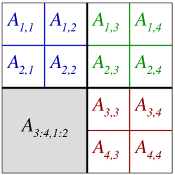
In order to discuss the implications of these two advanced features of OmpSs-2 on the $\mathcal{H}$-LU factorization, let us consider the re-partitioning of the initial sample matrix $A$ as shown in Figure 3. (Compared with the initial case in Figure 1, an additional $2\times 2$ partitioning has been imposed here on the top-right block $A_{1:2,3:4}$.) Correspondingly, the initial update (see the sequence of operations for the $\mathcal{H}$-LU factorization in Section 3)

$$\begin{array}[]{rrcl}\mbox{{\sf\small O2}}:&U_{1:2,3:4}&:=&L_{1:2,1:2}^{-1}A_{1:2,3:4}\end{array}$$

can be further decomposed into the six suboperations:

$$\begin{array}[]{rrcl}\mbox{{\sf\small O2.1}}:&U_{1,3}&:=&L_{1,1}^{-1}A_{1,3},\\[5.78172pt] \mbox{{\sf\small O2.2}}:&U_{1,4}&:=&L_{1,1}^{-1}A_{1,4},\\[5.78172pt] \mbox{{\sf\small O2.3}}:&A_{2,3}&:=&A_{2,3}-L_{21}\cdot U_{1,3},\\[5.78172pt] \mbox{{\sf\small O2.4}}:&A_{2,4}&:=&A_{2,4}-L_{21}\cdot U_{1,4}\\[5.78172pt] \mbox{{\sf\small O2.5}}:&U_{2,3}&:=&L_{2,2}^{-1}A_{2,3},\quad\mbox{\rm and}\\[5.78172pt] \mbox{{\sf\small O2.6}}:&U_{2,4}&:=&L_{2,2}^{-1}A_{2,4}.\end{array}$$

In the application of nested parallelism to this scenario, we again assume that O1, O2, O3, O4, O5 are each annotated as a (coarse-grain) task, and the decompositions of O1, O2, O5 respectively produce the operations in O1.1–O1.5, O2.1–O2.6, O5.1–O5.5, each annotated as a (fine-grain) task.

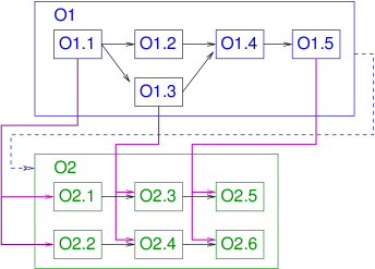
A rapid analysis of the new scenario reveals that, for example, the coarse-grain dependency O1$\rightarrow$O2 boils down (among others) to the finer-grain cases O1.1$\rightarrow${O2.1, O2.2}, as the former operation (LU factorization)

$$\begin{array}[]{rrcl}\mbox{{\sf\small O1.1}}:&A_{1,1}&:=&L_{1,1}U_{1,1}\end{array}$$

yields the unit lower triangular factor $L_{1,1}$ required by the latter two operations (triangular solves) O2.1, O2.2.

The problem with OmpSs and OpenMP 4.5 is that ensuring a correct result requires the introduction of a taskwait at the end of the code of O1 in order to guarantee a correct result. In contrast, the support for weak dependencies and early release in OmpSs-2 implies that (provided the operand $L_{1:2,1:2}$ for O2 is annotated as weak,) the boundaries between the coarse-grain tasks O1 and O2 can be crossed and the execution of O2.1 and O2.2 can commence as soon as O1.1 is computed. In order to attain this effect, in OmpSs-2 we should annotate O2 as a task with weak operands (via the corresponding representants):

⬇

1#pragma oss task weakin( RepL[0;S] ), weakinout( RepB[0;S] )

2void task_ltrsm( int M, int P, double *L, int LDL,

3 double *B, int LDB )

while O2.1, O2.2 are both specified as tasks with strong operands:

⬇

1#pragma oss task in( L[0;M*M] ), inout( B[0;M*P] )

2void task_ltrsm( int M, int P, double *L, int LDL,

3 double *B, int LDB )

This simple example illustrates that the use of weak dependencies and early release can unleash a higher degree of task-parallelism during the execution of the $\mathcal{H}$-LU factorization as, for example, the execution of O2.1, O2.2 can proceed in parallel with that of O1.2–O1.5; and O2.3, O2.4 in parallel with O1.2, O1.4, O1.5; see Figure 4.

Figure 4: Data dependencies between tasks O1 and O2 of the blocked RL algorithm for the $\mathcal{H}$-LU factorization. The black solid lines specify “internal” strong dependencies; the pink solid lines, strong dependencies crossing task boundaries; and the blue dashed line, the weak dependency.

6 Numerical Experiments

In this section we first describe the problem setup and target architecture employed in our experiment. Next we analyze the concurrency of the parallel implementations of the code for the $\mathcal{H}$-LU factorization in H2Lib.

6.1 Mathematical problems

The usage of $\mathcal{H}$-matrices often appears in the context of Boundary Element Methods (BEM) [15]. The reason for this is that the discretization of boundary integral equations often yields matrices that are densely populated and have to be stored efficiently, where $\mathcal{H}$-matrices come in handy. There is also a need of constructing efficient preconditioners for this type of equations, which can be carried out in $\mathcal{H}$-arithmetic. In particular, in the experiments in this section we consider integral equations of the form

$$\int_{\Gamma}g(x,y)\,u(y)\,dy=f(x),\qquad\text{for almost all }x\in\Omega,$$

where $\Omega$ can be some $d$-dimensional bounded domain for $d\in\{1,2,3\}$. By choosing suitable test-and-trial spaces $\mathcal{U}_{h}$ and $\mathcal{V}_{h}$, equipped with some bases $\left(\varphi_{i}\right),i\in\mathcal{I}$, and $\left(\psi_{j}\right),j\in\mathcal{J}$, we can apply a Galerkin discretization and obtain a variational formulation of the kind

$$\int_{\Omega}v_{h}(x)\int_{\Gamma}g(x,y)\,u_{h}(y)\,dy\,dx=\int_{\Omega}v_{h}(x)\,f(x)\,dx\,,\qquad\text{for all }v_{h}\in\mathcal{V}_{h}.$$

Employing finite element basis functions for these spaces we directly obtain a system of linear equations

$$Gu=f,$$

where all the entries of the matrix

$$g_{ij}=\int_{\Omega}\varphi_{i}(x)\int_{\Gamma}g(x,y)\,\psi_{j}(y)\,dy\,dx\,,\qquad\text{for all }i\in\mathcal{I},j\in\mathcal{J},$$

are non-zero.

In particular, we consider the Laplace equation in $d\in\{1,2,3\}$ dimensions. In these cases the underlying kernel functions are

$$g:\mathbb{R}^{d}\times\mathbb{R}^{d}\to\mathbb{R}\,,\quad g(x,y)=\begin{cases}-\log|x-y|&:d=1,\\ -\frac{1}{2\pi}\log\|x-y\|_{2}&:d=2,\\ \frac{1}{4\pi}\|x-y\|_{2}^{-1}&:d=3.\end{cases}$$

For the construction of low-rank blocks within our experiments, we choose the analytical method of tensor-interpolation [16], which is applicable in all dimensions. For the sake of lighter storage requirements and faster setup times of the $\mathcal{H}$-LU, we further re-compress all low-rank blocks by a fast singular value decomposition (SVD) [14].

6.2 Setup

All the experiments in this section were performed using ieee 754 double-precision arithmetic, on a single node of the MareNostrum 4 system at Barcelona Supercomputing Center. The node contains two Intel Xeon Platinum 8160 sockets, with 24 cores per socket, and 96 Gbytes per of DDR4 RAM. In Turbo frequency mode (3.7 GHz), the theoretical peak performance for a single core is 59.2 GFLOPS (billions of floating-point operations per second) when using AVX2 instructions. This rate is reduced to 33.6 GFLOPS when using a single core running in the base frequency (2.1 GHz). At this point we note that the aggregated (theoretical) peak performance of this machine is a linear function of the operation frequency which, in turn, depends on the specific type of vector instructions that are executed (AVX, AVX2, AVX-512) and the number of active cores [17].

In the experiments we employed gcc 4.8.5, Intel MKL 2017.4 (with AVX2 instructions enabled), and OmpSs-2 (mcxx 2.1.0).

6.3 Matrix-matrix multiplication

Our first experiment is designed to assess the performance of the implementation of the matrix-matrix multiplication routine (dgemm) in Intel MKL. This is relevant because it offers an upper bound of the actual performance that can be obtained from the $\mathcal{H}$-LU factorization of a hierarchical matrix. This bound will be tight in case most of the blocks involved in the decomposition are dense and the fragmentation of the blocks implicit to the matrix hierarchy is not too fine-grained.

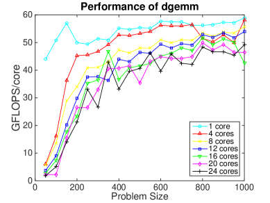
Figure 5 reports the GFLOPS per core attained by Intel’s dgemm routine using 1, 4, 8,…, 24 cores (of a single socket) and square operands all of the same dimension $b$. (Note that the limit of the $y$-axis in this plot and all subsequent ones is fixed to 60, which basically corresponds to the theoretical peak performance with 1 core.) This experiment reveals two important aspects. First, the execution of the sequential instance of dgemm delivers 57.0 GFLOPS for a problem of order $b=150$, and 58.9 GFLOPS for the largest problem dimension, $b=1000$. These values represent 96.2% an 99.4% of the peak rate, respectively (when using AVX2 instructions). Thus, even for problems that are rather small, it is already possible to attain a large fraction of the peak performance when using a single thread. Second, as the number of threads/cores grows, the multi-threaded instance of dgemm requires considerably larger problems to attain a relevant fraction of the theoretical peak. (As argued earlier, the peak rate of this processor is “variable” because it depends on the operation frequency and this parameter is constrained by the number of active cores [17].)

Figure 5: Performance of the matrix-matrix multiplication routine in Intel MKL.

6.4 Basic parallel solutions

The following experiment exposes the drawback of a parallelization that simply relies on a multi-threaded instance of the BLAS, providing initial evidence that a runtime-based approach can offer higher performance. In order to do so, we compare three different parallelization strategies applied to the $\mathcal{H}$-LU factorization:

• MKL extracts fine-grain loop-parallelism from within the BLAS kernels only. As argued in the introduction of this paper, this approach is rather appealing in that it requires a low programming effort. In particular, provided the sequential routine for the $\mathcal{H}$-LU factorization already casts most of its operations in terms of BLAS, the code can be executed in parallel by simply linking in a multi-threaded instance of this library such as that in Intel MKL. The downside of this approach is that it constrains the parallelism that can be leveraged to that inside individual kernels, which may be insufficient if the number of cores is large.

• OpenMP aims to exploit loop-parallelism (like MKL) but targets a coarser-grain layer, by applying the parallelization to the loops present in the $\mathcal{H}$-LU routine. To clarify this, consider for example a single-level hierarchical matrix that is decomposed into $8\times 8$ blocks. After the factorization of the leading block of the matrix, this approach will compute in parallel the remaining 7+7 triangular system solves in the same column+row of the matrix; and next update the $7\times 7$ blocks of the trailing submatrix in parallel. In summary, instead of extracting the parallelism from within the individual BLAS kernels, this approach targets the parallelism existing between independent BLAS kernels (tasks) comprised by a loop.

• OmpSs discovers tasks dynamically and takes into account the dependencies among them to schedule their execution when appropriate; see Section 4. (This version does not include the advanced features supported by OmpSs-2.)

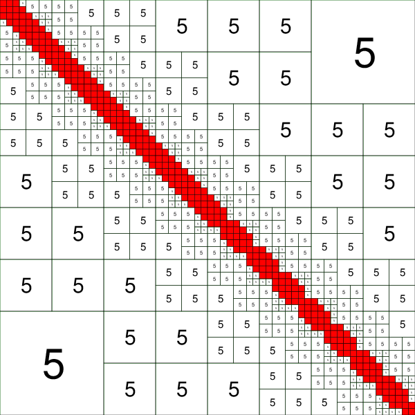
To simplify the following analysis, we will employ a hierarchical matrix with a $2\times 2$ recursive structure defined on the diagonal blocks. Concretely, starting with a hierarchical matrix of order $n$, we define a $2\times 2$ partitioning, which is recursively applied to the inadmissible blocks until a minimum leafsize is reached; see Figure 6. This type of data structure appears, for example, in BEM with $d=1$ as those described in subsection 6.1. For simplicity, we will also consider dense blocks only. With these consideration, the cost of the LU factorization of a hierarchical matrix of order $n$ is (approximately) the standard $2n^{3}/3$ flops.

Figure 6: Hierarchical structures of the $\mathcal{H}$-matrices employed in the evaluation of the parallelization strategies (with 5 recursive partitionings of the diagonal blocks; note that the colors remark the amount of levels defined in each structure: 7, 6, 5 and 4 respectively).

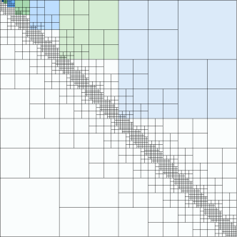
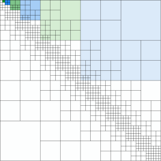
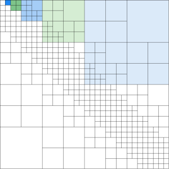
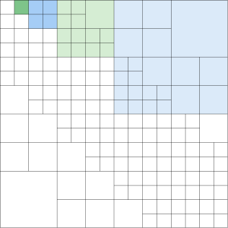
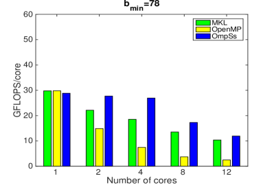
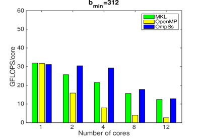
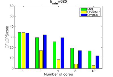
Figure 7 reports the GFLOPS per core for the three different parallelization strategies described above. The results there correspond to a square $\mathcal{H}$-matrix of dimension $n=10$K, with $r=4$, 5, 6 and 7 recursive partitionings applied to the inadmissible blocks until a minimum leafsize is reached. This implies that the smallest blocks on the diagonal are of order $b_{\min}=10\mathrm{K}/2^{r}\approx 625$, 312, 156 and 78, respectively. This experiment offers some interesting insights:

• The performance of MKL greatly benefits from problems with large block sizes, which is consistent with the trends in the GFLOPS rates observed for the multi-threaded instance of Intel’s dgemm in the previous experiment. This option is competitive with the task-parallel OmpSs-based routine when the number of cores is reduced or partitioning features large diagonal blocks ($r=4$, $b_{\min}=625$).

• The parallel performance of OpenMP is practically negligible as the GFLOPS per core decrease linearly with the number of cores. This is not totally a surprise as, due to the $2\times 2$ organization of the $\mathcal{H}$-matrix, the operations that can be performed independently are reduced to the two triangular system solves at each partitioning.

• When the number of cores is small, the OmpSs-based parallelization attains mild GFLOPS rates. Here, the coarse-grain partitioning of the blocks and the existence of synchronization points constrain the degree of parallelism that can be exploited and limit the performance of this approach when the number of cores is large.

Figure 7: Performance of basic parallelization strategies applied to an $\mathcal{H}$-matrix of order $n=10$K, with dense blocks, and a recursive $2\times 2$ hierarchical partitioning of the inadmissible blocks; see Figure 6.

To complete the analysis of this experiment, we remark that a comparative analysis of the GFLOPS observed in these executions with those of dgemm is delicate. In particular, the execution using a single core can be expected to set the processor to operate on a higher frequency than a parallel multi-threaded execution using several cores. Unfortunately, the exact frequency is difficult to know as it depends on the number of cores as well as the arithmetic intensity of the operations (and it can even vary at execution time).

6.5 Scalability of task-parallel routines

Our next experiments aim to demonstrate the benefits that the WD+ER (weak dependency and early release) mechanism exerts on the scalability of the task-parallel codes based on OmpSs-2. For this purpose, we next conduct an analysis of the strong and weak scalabilies, using a complete socket (24 cores) and the same hierarchical matrix, with a $2\times 2$ recursive structure defined on the diagonal blocks and dense blocks only, employed in the previous study.

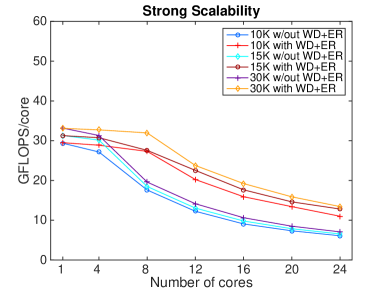
In the following analysis of strong scalability, we set the problem dimension to three different values, $n=$10K, 15K and 30K, and progressively increase the amount of cores up to 24 while measuring the GFLOPS per core. In this type of experiment, we can expect that the GFLOPS/core rates eventually drop as the problem becomes too small for the volume of resources that are employed to tackle it. Figure 8 confirms that this is the case for both implementations, which exploit/do not exploit the new features in OmpSs-2 (lines labeled as with WD+ER and w/out WD+ER, respectively). In addition, the results also show that the exploitation of WD+ER, made possible by OmpSs-2, offers a GFLOPS/core rate that clearly outperforms that of the implementation that is oblivious of these options.

Figure 8: Strong scalability of the advanced parallelization strategies applied to $\mathcal{H}$-matrices of order $n=10$K, 15K and 30K ($b_{\min}=$156, 234 and 234, respectively), with dense blocks, and a recursive $2\times 2$ hierarchical partitioning of the inadmissible blocks; see Figure 6.

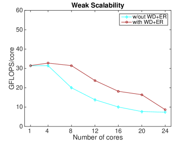
For the analysis of weak scalability, we utilize a problem of dimension $n\times n$ that grows proportionally to the number of cores $c$, so that the ratio $n^{2}/c=15$K$\times 15$K holds while $c$ grows to 24. As the problem size per core is constant, we can expect that the GFLOPS/core remains stable, showing the possibility of addressing larger problems by increasing proportionally the amount of resources up to a certain point. (This is not totally exact, as the cost of the factorization for dense matrices grows cubically with the problem dimension while, in the conditions set for this experiment, the amount of resources only does so quadratically.) Unfortunately, the results of this experiment reveal that the weak scalability of both algorithms suffers an important drop as the number of cores is increased, though in the variant equipped with WD+ER this occurs in the transition from 8 to 12 cores while the implementation that does not exploit this mechanism the gap is visible already in the increase from 4 to 8 cores.

There are two aspects to take into account when considering the GFLOPS/core rates observed in the strong scaling analysis and, especially, the weak scaling counterpart. The first one refers to the CPU frequency, which decreases with the number of cores which are active (see [17] and Figure 5) and affect the performance of the task-parallel routines, reducing it with the number of cores. The second one is a consideration of the structure of the hierarchical matrix employed in these experiments (see Figure 6). In particular, when all the blocks are dense, and the matrix is decomposed into a task per block in this partitioning, the result is a problem where a reduced collection of coarse-grain tasks concentrate a large fraction of the flops. This effect is exacerbated with the problem order ($n$) and its negative effect is more visible when the number of cores is increased because the task-parallel algorithms confront then a suboptimal scenario consisting of a very reduced number of tasks (little task-parallelism) of (very) coarse-grain operations.

Figure 9: Weak scalability of the advanced parallelization strategies applied to an $\mathcal{H}$-matrix of dimension $n\times n=15$K$\times 15$K per core ($b_{\min}=$234 in all cases, except with 8 cores where $b_{\min}=$166), with dense blocks, and a recursive $2\times 2$ hierarchical partitioning of the inadmissible blocks; see Figure 6.

6.6 Parallelism of task-parallel routines with low-rank cases

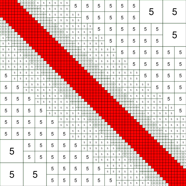
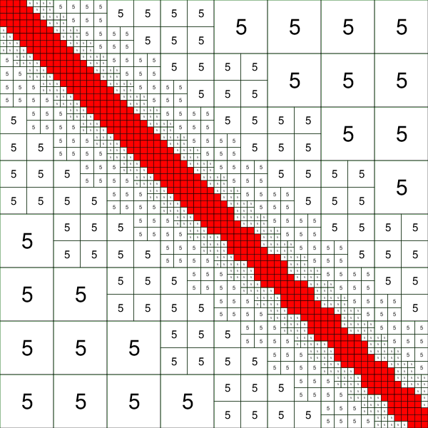
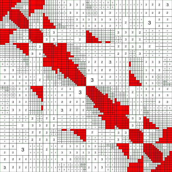
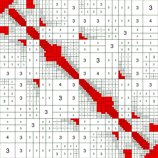
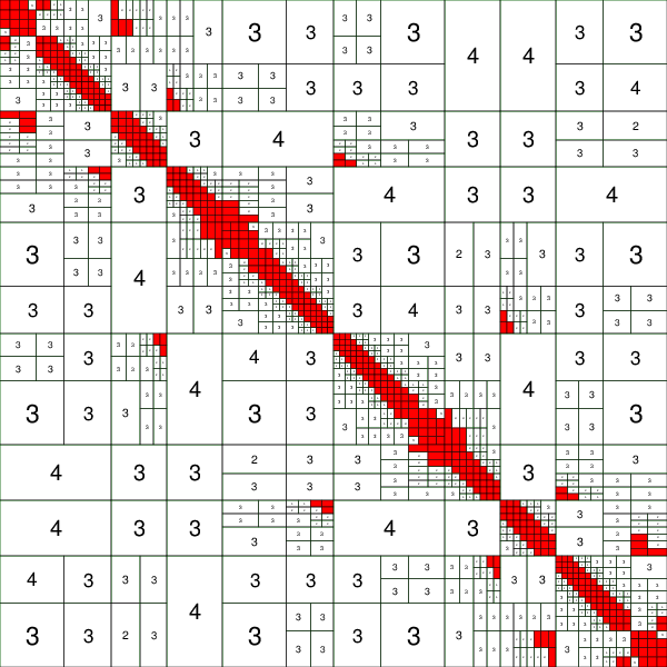
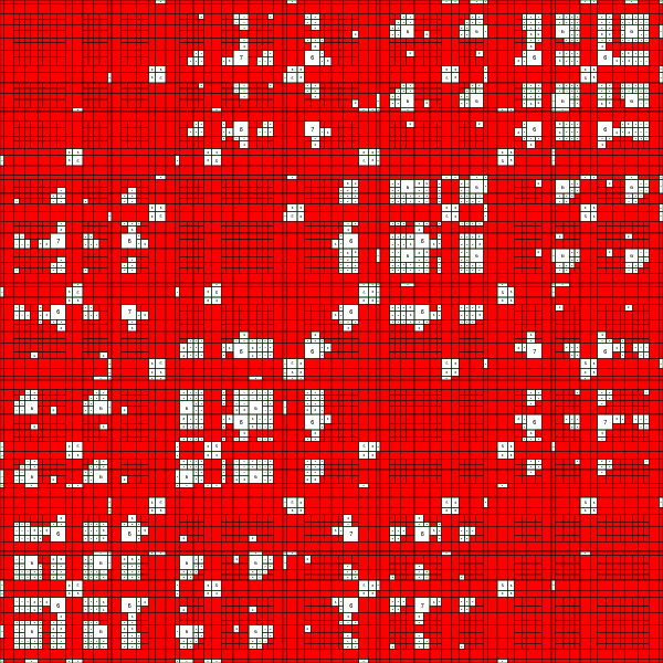
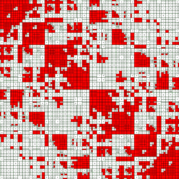
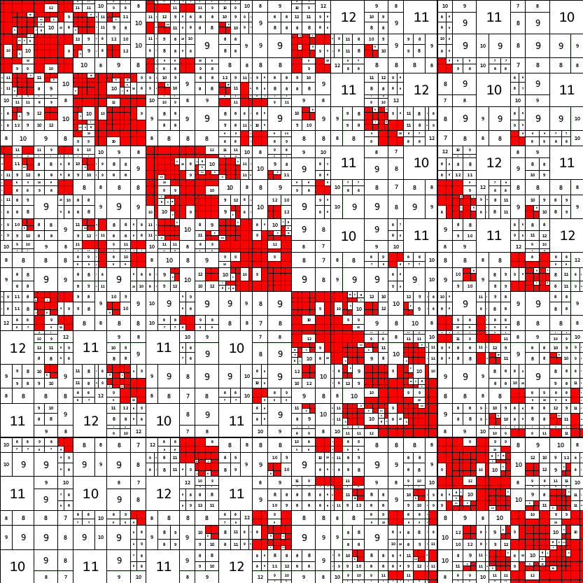
Our final round of experiments assesses the performance of the WD+ER (weak dependency and early release) mechanism using several BEM cases, of dimensions $d=$1, 2 and 3, involving low-rank blocks. The “sparsity” pattern of these blocks is controlled via a parameter $\eta$ that we set to four different values, 0.25, 0.5, 1.0 and 2.0. The structure of these cases is illustrated in Figure 10.

Figure 10: Hierarchical structure of the $\mathcal{H}$-matrix employed in the evaluation of the task-parallel routines. The red areas denote dense blocks and the number inside the white blocks specifies the rank of the corresponding (low-rank) block. From top to bottom: $d=$1, 2 and 3; and from left to right: $\eta=$0.25, 0.5, 1.0 in the first two rows, and $\eta=$0.5, 1.0, 2.0 in the last one.

Table 1 reports the acceleration factors (or speed-ups) attained by the task-parallel codes with respect to the corresponding sequential code/case, using problems of order $n\approx 30$K and up to 24 cores. This final experiment illustrates the performance advantage of exploiting the WD+ER also in case of $\mathcal{H}$-matrices with low-rank blocks. In general, the speed-up increases with the ratio of dense blocks, reporting notably high values for $d=1$ and 3 (provided the number of cores is not too large compared with the problem dimension), and much lower for those cases with $d=2$. In some cases we even observe a super-linear speed-up, due to cache effects.

		WD+	Seq.	Speed-up with #cores
$\eta$	$d$	ER?	time	4	8	12	16	20	24
0.25	1	No	89.2	3.51	5.24	5.58	5.70	5.70	5.69
		Yes		4.05	7.82	11.56	14.62	17.37	19.04
	2	No	118.9	3.70	6.12	7.28	7.79	7.88	8.02
		Yes		3.96	7.64	10.99	13.55	17.36	18.49
0.50	1	No	38.1	2.60	2.74	2.73	2.71	2.71	2.70
		Yes		3.92	7.45	9.57	9.74	9.69	9.45
	2	No	37.0	3.04	3.68	3.82	3.90	5.74	3.92
		Yes		3.96	6.87	8.81	9.68	10.18	10.44
	3	No	1,099.2	4.00	7.83	13.48	14.44	16.88	18.71
		Yes		4.00	7.99	11.85	15.63	19.13	21.57
1.00	1	No	12.6	1.55	1.58	1.57	1.57	1.56	1.57
		Yes		2.50	2.46	2.48	2.46	2.44	2.43
	2	No	12.0	1.92	1.99	2.00	2.00	1.99	2.00
		Yes		3.31	4.22	4.38	4.50	4.44	4.36
	3	No	1,049.8	3.96	7.54	10.84	13.28	15.64	17.63
		Yes		4.03	7.91	14.32	15.55	18.99	21.73
2.00	3	No	204.1	3.59	5.78	7.39	7.88	8.26	8.44
		Yes		4.99	7.87	11.27	14.65	17.33	17.83

Table 1: Execution time of the sequential algorithm in H2Lib (in sec.) and parallel speed-up of the advanced parallelization strategies applied to an $\mathcal{H}$-matrix of order $n\approx 30$K ($b_{\min}=$234), with dense and low-rank blocks; see Figure 10.

7 Concluding Remarks

We have demonstrated notable parallel efficiency for the calculation of the $\mathcal{H}$-LU factorization on a state-of-the-art Intel Xeon socket with 24 cores. A key component to attain this high performance is the exploitation of weak dependencies and early release, recently introduced in OmpSs-2. Armed with these mechanisms, the OmpSs-based parallel codes can cross the dependency domains, discovering and exploiting a notably higher degree of task-parallelism, which results in higher performance in the execution of 1D, 2D and 3D cases arising from BEM. As part of future work, we would like to investigate hybrid parallelization schemes that combine the extraction of multi-threaded parallelism from highly tuned libraries such as Intel MKL with task-parallelism exploited by a runtime. Moreover, we will investigate new strategies to extract additional levels of task-parallelism.