The envelope of the semiregular variable V CVn
Abstract
V CVn is a semiregular variable star with a –band amplitude of mag. This star has an unusually high amplitude of polarimetric variability: up to 6 per cent. It also exhibits a prominent inverse correlation between the flux and the fraction of polarization and a substantial constancy of the angle of polarization. To figure out the nature of these features, we observed the object using the Differential Speckle Polarimetry at three bands centered on 550, 625 and 880 nm using the 2.5-m telescope of Sternberg Astronomical Institute. The observations were conducted on 20 dates distributed over three cycles of pulsation. We detected an asymmetric reflection nebula consisting of three regions and surrounding the star at the typical distance of 35 mas. The components of the nebula change their brightness with the same period as the star, but with significant and different phase shifts. We discuss several hypotheses that could explain this behavior.
keywords:
stars: oscillations – circumstellar matter – instrumentation: high angular resolution.1 Introduction
The radiation of red long–period variables (LPV) is often polarized due to scattering on the dust, which is being formed in their relatively cool atmospheres. The fraction and angle of polarization of LPV fluctuate randomly due continuous chaotic changes in the envelopes of these object. Usually the fraction of polarization changes from 0 to 2 per cent, the orientation of the polarization plane has no preferred direction (Clarke, 2010). A semiregular variable star V CVn, which has a period of days (Samus’ et al., 2017) and –band amplitude of mag, stands out against this background. The fraction of polarization of this star changes from 1 to 6 per cent while the angle of polarization is quite stable: from to (Serkowski & Shawl, 2001). In addition, V CVn exhibits most prominent inverse correlation between flux and fraction of polarization among other long–period variables.
Neilson et al. (2014) discussed the polarization variability of V CVn in detail. They considered qualitatively several hypotheses which can potentially describe unique behavior of the star. They concluded that the model of dusty disc and the model of bow shock are the most probable. In the first case, the intrinsic polarization is generated by the scattering from the dusty thick disc or torus. The observer is close to the plane of equator of this structure. The second hypothesis states that a bow shock is formed at the boundary between the stellar wind of V CVn and the interstellar medium, similar to one found around Ceti (Martin et al., 2007). Dust from the wind will be accumulated at this boundary. This dusty structure will also scatter and polarize stellar radiation.
In both cases an asymmetry of scattering envelope emerges. It can potentially produce non–zero intrinsic polarization of the object and the constancy of polarization angle. Neilson et al. (2014) showed how the inverse correlation between the total flux and polarization of the object can be qualitatively explained by the interaction between the pulsation–driven density waves and the bow shock or dusty disk.
The existing array of polarization measurements of V CVn covers dozens of pulsation cycles, what allows to state that the peculiar behavior of the object is being reproduced. However in these measurements the polarization of the whole object was integrated hampering further interpretation. The localization of polarized flux source or sources may be the key to understanding of the object.
Here we report on the observations of V CVn using a high angular resolution polarimetry technique. We detected a circumstellar environment around the star, which behaviour may explain polarimetric variability of the object. The paper is organized as follows. We briefly describe a method and observations in Section 2. In Section 3 we construct a simple geometric model of the observations. The discussion of possible interpretations and conclusions are provided in Sections 4 and 5, respectively.
2 Observations
V CVn was observed using the SPeckle Polarimeter (SPP) of the 2.5-m telescope of the Caucasian Observatory of the Sternberg Astronomical Institute of Lomonosov Moscow State University. The SPP is a combination of a two–beam polarimeter and a speckle interferometer (Safonov et al., 2017). The instrument is aimed at the study of polarization of astrophysical objects at diffraction limited angular resolution, i.e. 50 mas at wavelength of 500 nm. The angular scale of SPP camera is 20.6 mas pix-1.
The observations were conducted on 18 dates distributed from 2017 December 2 to 2019 January 20 in the fast polarimetry regime using three medium–band filters centered on 550, 625, and 880 nm. In addition, we observed the object in filters and on two dates in the spring of 2017.
The data were reduced using the Differential Speckle Polarimetry (DSP) method described by Safonov et al. (2019). As a result, we obtained estimations of the visibility ratios of the object in orthogonally polarized light (Norris et al., 2012):
| (1) |
Here , , and are the Fourier transforms of the Stokes parameters distributions in the object. is the spatial frequency. As one can see, it is possible to define two ratios: and for the Stokes parameters and , respectively. DSP allows to estimate both the amplitude and phase of value. The observations were conducted at the Cassegrain and Nasmyth foci of the telescope. In the case of the Nasmyth focus the correction for the instrumental polarization effects was applied (Safonov et al., 2019).
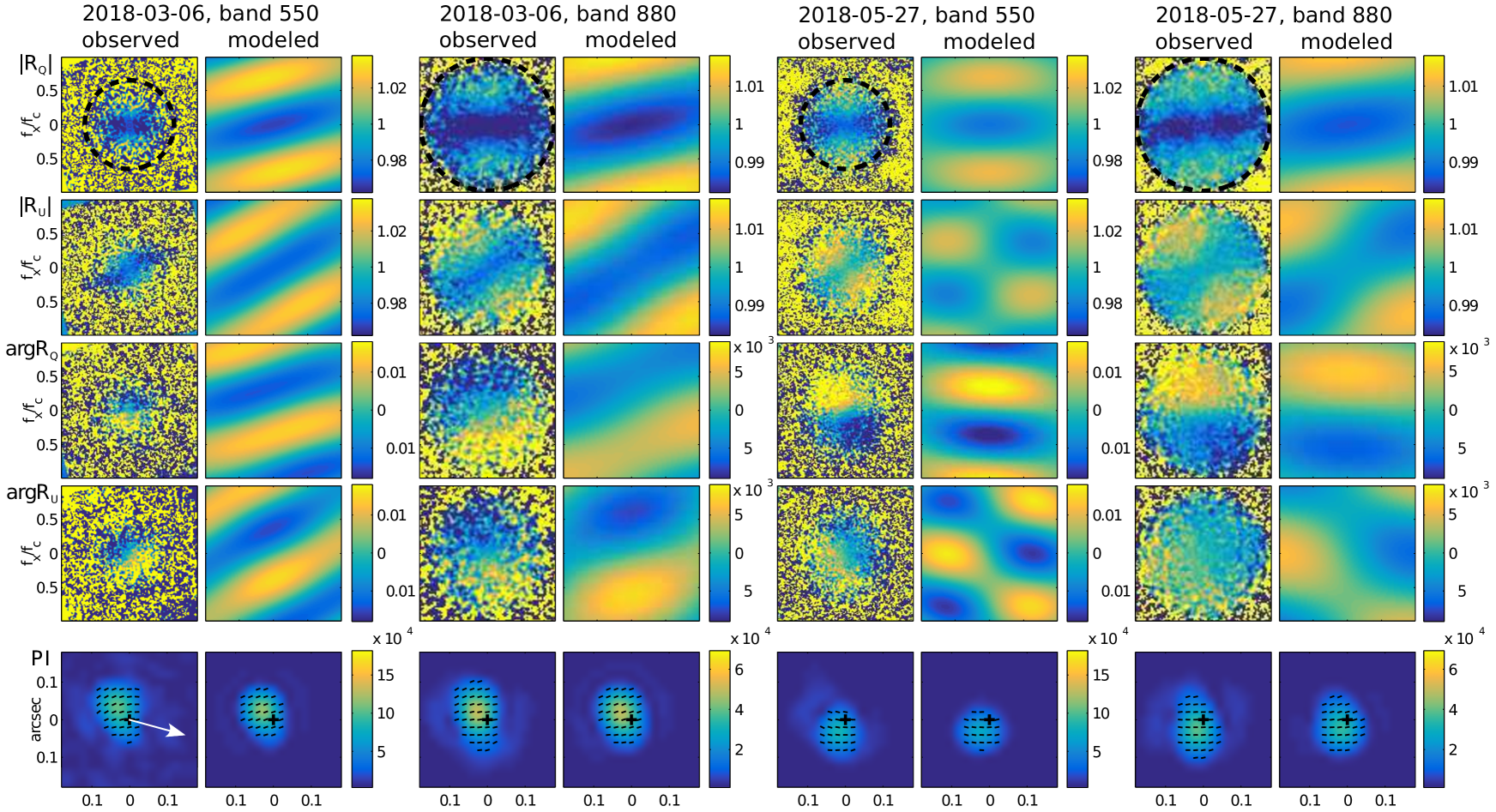
The measurements of value for the two dates and two filters are presented in Fig. 1. The polarized flux was clearly resolved for these cases as long as values deviate from unity significantly.
Safonov et al. (2019) demonstrated how the distribution of Stokes parameters in some object can be estimated from the value measurements. The polarized intensity computed using this method is displayed in the bottom row of Fig. 1.
The polarization of each elementary area of the envelope is roughly perpendicular to the direction connecting this area and the star. Therefore this envelope is likely to be a reflection nebula surrounding the star. The results of observations conducted on the same dates but at different filters are in good agreement. On the other hand, the difference between the observations conducted on two dates is striking. The nebula was dominated by the feature at north–northeast of the star on March 5th. 82 days later, on May 27th, the feature at south–southeast became significantly brighter than the northern one. For some other dates the feature at south–southwest became prominent. The images similar to Fig. 1 for all filters and all dates are provided at http://lnfm1.sai.msu.ru/kgo/mfc_VCVn_en.php.
The detected nebula has a characteristic angular size comparable to the diffraction–limited resolution of the telescope. The appearance of the images in polarized intensity is strongly affected by the blurring by the PSF. Due to this and some others problems discussed by Safonov et al. (2019), these images can only be analyzed qualitatively. For the quantitative interpretation of the observations we will compare model and observations in terms of .
3 MODELLING
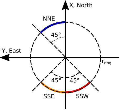
Judging by the polarized intensity images of V CVn for all dates, the simplest model for this source appears to be an unpolarized central star surrounded by three scattering arcs, see Fig. 3. The configuration of the arcs is fixed. We will denote these arcs in accordance with their position relative to the star: north–northeast (NNE), south–southeast (SSE), and south-southwest (SSW). The radius is assumed to be the same for all arcs. Each elementary interval of the arcs is polarized perpendicularly to the direction connecting this interval and the star.
In the frame of this model a single observation can be described by 4 parameters: the radius of the arcs and ratios of their polarized fluxes to the total flux of the object: . The polarized flux is the product of polarization fraction and the total flux. These parameters defines the distribution of Stokes parameters in the object, from which we computed the expected and (1). We emphasize that in the frame of method which we use it is impossible to estimate the polarization fraction of arc and its total flux. We can estimate only their product: polarized flux.
To compare the modelled and observed values, we calculated a total residual weighted by , where is the uncertainty of determination (Safonov et al., 2019). The residual was summed in the frequency domain, where the signal–to–noise ratio in is sufficiently high, see Fig. 1. The optimal model was found by minimizing the total residual.
We assumed that the arc’s radius does not depend on time and wavelength. It was determined by the approximation of the observations at three filters conducted on two dates: 2018 Mar 6th and 2018 May 27th. We found the radius to be mas. As long as is less than formal diffration limited resolution of the telescope, its value is model–dependent. For example, it would be different for the model of sectors, not arcs. Nevertheless the departure of polarized envelope from the point–like star is detected quite reliably, and can be considered as its characteristic angular extent.
We fixed the radius of arcs at mas and approximated each observation individually varying the rest three parameters . The examples of modelled values and the corresponding images are displayed in Fig. 1. The agreement with the observations is reasonable. The results of approximation of all observations are provided in Table 1. The statistics is less than 3 for 39 observations out of 57. Thus for most observations the model describes the observations satisfactorily.
The total polarized flux from the envelope amounts to 0.01-0.03 of total flux of the object. In other words, the envelope explains the polarization of the object, while the unpolarized flux from the star dominates total the flux.
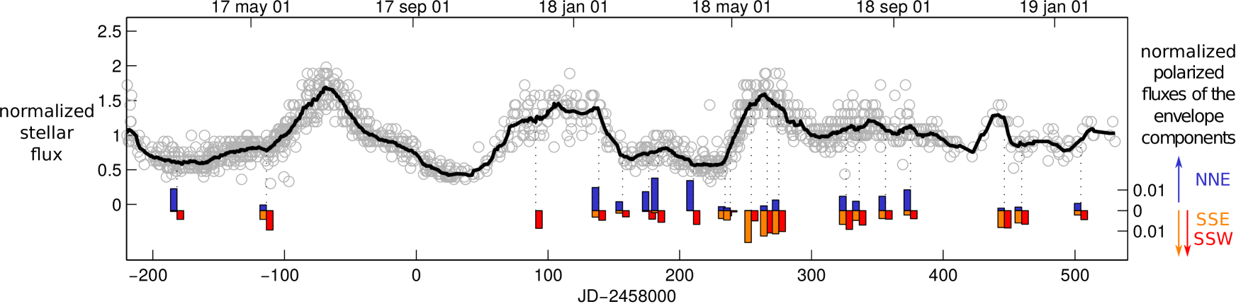
The Fig. 2 displays the behaviour of the components of the envelope in and 550 filters. For ease of comparison, the AAVSO light curve (Kafka, 2018) is given on the same graph. Note that the polarized fluxes of the envelope’s arcs are normalized by the average flux of the object. This allows to inspect the variability of the arcs independently of the variability of the star.
It follows from Fig. 2 that the brightening of the arc NNE coincides with the minimum brightness of the whole object. This leads to rise of the total polarization of the object. At the same time the arcs SSE and SSW change their brightness synchronously with the star.
| polarized flux, | ||||||||
|---|---|---|---|---|---|---|---|---|
| JD | filter | mag | ,% | NNE | SSE | SSW | ||
| 2457818.4 | 8.00 | 2.1 | ||||||
| 3.80 | 13.9 | |||||||
| 2457886.2 | 7.50 | 1.9 | ||||||
| 3.60 | 9.6 | |||||||
| 2458090.6 | 7.10 | 1.7 | ||||||
| 5.90 | 2.0 | |||||||
| 3.70 | 3.0 | |||||||
| 2458138.6 | 7.10 | 9.0 | ||||||
| 5.80 | 0.9 | |||||||
| 3.30 | 2.8 | |||||||
| 2458156.6 | 7.80 | 1.6 | ||||||
| 6.40 | 1.6 | |||||||
| 3.70 | 6.3 | |||||||
| 2458176.6 | 7.50 | 1.3 | ||||||
| 6.30 | 1.5 | |||||||
| 3.70 | 4.2 | |||||||
| 2458183.6 | 7.40 | 1.0 | ||||||
| 6.30 | 1.1 | |||||||
| 4.00 | 1.9 | |||||||
| 2458210.3 | 7.70 | 1.5 | ||||||
| 6.80 | 1.4 | |||||||
| 4.00 | 2.9 | |||||||
| 2458234.4 | 7.50 | 2.8 | ||||||
| 6.40 | 2.3 | |||||||
| 3.60 | 5.8 | |||||||
| 2458238.4 | 7.40 | 3.9 | ||||||
| 5.90 | 2.7 | |||||||
| 3.50 | 8.2 | |||||||
| 2458254.4 | 6.80 | 1.2 | ||||||
| 5.60 | 1.4 | |||||||
| 3.30 | 2.9 | |||||||
| 2458266.4 | 6.90 | 2.6 | ||||||
| 5.50 | 3.3 | |||||||
| 3.60 | 3.2 | |||||||
| 2458275.3 | 6.80 | 1.4 | ||||||
| 5.70 | 1.6 | |||||||
| 3.60 | 4.8 | |||||||
| 2458326.2 | 7.00 | 1.2 | ||||||
| 6.10 | 2.4 | |||||||
| 3.60 | 15.8 | |||||||
| 2458336.2 | 7.10 | 0.9 | ||||||
| 6.00 | 1.2 | |||||||
| 3.70 | 8.2 | |||||||
| 2458356.2 | 7.20 | 1.7 | ||||||
| 6.00 | 2.5 | |||||||
| 3.80 | 11.4 | |||||||
| 2458375.2 | 7.40 | 1.6 | ||||||
| 6.20 | 1.9 | |||||||
| 3.90 | 5.2 | |||||||
| 2458446.5 | 7.00 | 1.5 | ||||||
| 6.00 | 1.4 | |||||||
| 3.60 | 3.6 | |||||||
| 2458459.6 | 7.30 | 1.1 | ||||||
| 6.00 | 1.4 | |||||||
| 3.50 | 4.0 | |||||||
| 2458504.5 | 7.10 | 3.0 | ||||||
| 6.00 | 3.2 | |||||||
| 3.50 | 9.5 | |||||||
These features were roughly reproduced at the considered cycles of pulsation. The exact repetition is not expected anyway, because the pulsation of the star is irregular. For example, in the period of pulsation between JD=2458260 and JD=2458440 there was no prominent minimum of brightness on the light curve. The polarization fraction stayed below 2 per cent. The difference in arcs brightnesses in that period was less pronounced with respect to the previous minimum. Nevertheless the overall character of the arcs brightnesses variability was the same.
4 DISCUSSION
In accordance with the latest measurements of Gaia Collaboration et al. (2018) the distance to V CVn is kpc. The star resides quite high above the galactic plane: kpc. The apparent proper motion of V CVn is mas yr-1 and mas yr-1, the correspoding tangential velocity is 251 km s-1 with respect to the Sun. The radial velocity is 4.7 km s-1 (Famaey et al., 2009), i.e. the star travels almost perpendicularly to the line of sight.
The parallax of V CVn is determined with error of 0.14 mas, what is three times larger than the median of this value for stars with (Lindegren et al., 2018). The error of proper motion is relatively large as well. The excessive noise of astrometrical solution can be caused either by chromatic instrumental effects inherent to Gaia data, or by the envelope described in previous section.
Sharma, Prugniel & Singh (2016) provide the following fundamental parameters of the star: the spectral type is M6III, the effective temperature is K. The luminosity corresponding to the Gaia distance is (McDonald, Zijlstra & Boyer, 2012). One can also estimate the radius of the star: , which results in the angular radius of 2.2 mas at the distance of the object.
The characteristic linear radius of the found nebula is au, what is times larger than . Therefore the observed polarized flux is formed in the circumstellar envelope at a significant distance from the photosphere. Most likely this envelope is generated by the dusty stellar wind. Mid–IR excess in the spectrum of V CVn (Price et al., 2010) and the 9.7 m silicate feature also favour the existence of a dusty envelope (Olnon et al., 1986; Simpson, 1991). At the same time the star has quite low colour excess (Montez et al., 2017) which indicates that the envelope is not spherically symmetric.
The Keplerian motion is the most obvious potential explanation for the observed changes in the morphology of the envelope. However getting across the semicircle with the radius of au in half the period of pulsation (P194 days Samus’ et al. 2017) requires a velocity of km s-1. This is much larger than the expected Keplerian velocity at au from the star with the mass less than . Therefore the hypothesis of Keplerian is rejected. In below we consider several other hypotheses for the interpretation of the V CVn envelope.
4.1 Bow shock hypothesis
(Neilson et al., 2014) proposed that the asymmetric dusty envelope could form behind the bowshock emerging at the boundary between stellar wind and the interstellar medium (ISM). The distance between the star and an apex of the bow shock is defined by the equality of ram pressures of the stellar wind and of the flow of the ISM gas (van Buren & McCray, 1988). Now we estimate at which density of ISM the bow shock will be located at 44 au from the star.
First we need a mass–loss rate of the stellar wind. This value can be estimated from the pulsation period using the relation by De Beck et al. (2010). In the case of V CVn the expected mass–loss rate is yr-1.
For the estimation of velocity of the star relative to the ISM we performed the correction for the differential rotation of the Galaxy and for the motion of the Sun towards the apex. We used the maser rotation curve, which is closest to the kinematics of the gas (Rastorguev et al., 2017). The velocity of the star with respect to the local rest frame is km s-1. The position angle of velocity vector projection on the image plane is , this direction is indicated by the arrow in the lower left panel of the Fig. 1.
Knowing the velocity of the star relative to ISM, and using equation (1) from (van Buren & McCray, 1988), it is possible to derive the following dependence of the required ISM density on the velocity of the stellar wind :
| (2) |
Here is expressed in km s-1, and is expressed in cm-3. The density of ISM is expected to be cm-3 at the terminal stellar wind velocity of a few km s-1, which is typical for this type of stars.
At the same time the average density of ISM at 1.2 kpc above the galactic plane is cm-3 (“best estimate” from fig. 10 in Dickey & Lockman 1990). In accordance with the map of H i obtained by Ben Bekhti et al. (2016) no significant molecular cloud exists towards V CVn. We conclude that the ISM in the vicinity of V CVn is by orders of magnitude less dense than required to form the bow shock at 44 au from the star.
In other words, the bowshock has to form at the distances much larger than the size of the detected envelope. But intrinsically spherical stellar wind should retain this symmetry up to distances where the bowshock is formed. Therefore in our case the interaction between stellar wind and ISM should not induce asymmetry of dusty envelope, and, moreover, any variability of its surface brightness. It is more likely that the shape of the envelope is caused by the anisotropy of the stellar mass loss.
4.2 Light echo hypothesis
The fact that the brightness of the NNE arc reaches its maximum value after days after the maximum of brightness of the star can be explained by the effect of the light echo, as in case of RS Pup (Kervella et al., 2008). In this case the NNE arc should be at least au farther from us than the star. The characteristic linear size of the cloud can be estimated as NNE arc length: au. The respective circumstellar cloud would intercept no more than of stellar radiation. Some of this radiation would be absorbed and the rest would be scattered mostly forward. For the observer the cloud would be seen in back–scattering regime as a source of polarized flux at least fainter than the star, i.e. fainter than observed — see Fig. 2. It means that the brightness of the detected nebula is inconsistent with the light echo hypothesis.
4.3 Variable shadowing hypothesis
Periodic changes in morphology of circumstellar envelope may be caused by the effect of variable shadowing. In this case the outer parts of the circumstellar envelope will be partly obscured from the point of view of the star by the inner parts of the same nebula. The geometry of this obscuration will depend on the radius of the star, which in turn changes with pulsation.
This hypothesis had been proposed by Kervella et al. (2014) to explain correlation between photocentre motion and pulsation cycle of another semiregular variable L2 Pup.
If this hypothesis is applicable to V CVn, then there is a structure in the inner envelope of the star which casts a shadow on NNE arc when the star is bright. Assuming that the star is larger at minimum brighness, and shadowing of NNE arc should decrease when the object is faint. Consequently, NNE arc should become brigther.
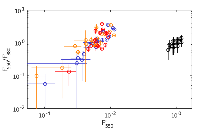
However the colour (temperature) of star depends on the pulsation cycle as well. Therefore in the frame of this explanation the tracks of the arcs in the colour–flux diagram should differ. The NNE arc should become more red at its brightening (when the star is faint), while SSE/SSW should become more blue, when they brighten.
But it follows from Fig. 4 that the colour behaviour of all components of the envelope is essentially the same and similar to one of the star: the bright state is characterized by the bluer colour. Therefore we reject this hypothesis as well.
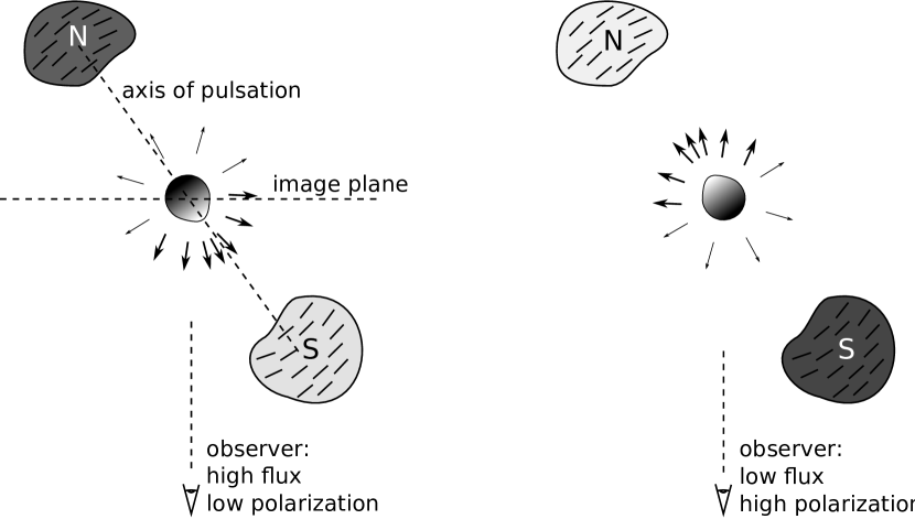
4.4 Non–radial pulsation hypothesis
The character of the variability of the NNE arc could be naturally explained in terms of the assumption that the pulsation of the star from its point of view is shifted by half a period relative to the pulsation from the point of view of the observer. At the same time from the point of view of SSW/SSE arcs the pulsation appears the same as for observer. The corresponding model is illustrated in Fig.5 and assumes significant departure of stellar pulsation from purely radial, or, more precisely, the existence of dipolar pulsation.
In the frame of this model, when the star at maximum brigthness, the part of star facing the observer and arcs SSW/SSE is in bright state. Meanwhile the part of star facing the arc NNE is faint. After the half a period of pulsation the situation is opposite. Now the star appears faint for the observer and bright for the NNE arc. Because of this the latter reaches maximum brighness. The input of scattered and polarized radiation in the total flux of the object rises. The inverse correlation between the total fraction of polarization and flux emerges.
Non–radial pulsation was considered as one of possible qualitative explanations for the unusual polarization variability of the star V1497 Aql by Patel et al. (2008). This semiregular variable star shows irregular changes in fraction of polarization with the amplitude of up to 5 per cent associated with relatively small changes in brighness . However, reliable evidences for non-radial pulsation giving an amplitude of are missing and theoretically it was not predicted (Mosser et al., 2013).
5 Conclusions
We have presented the observations of the semiregular variable V CVn using the method of differential speckle polarimetry at the wavelengths of 550, 625 and 880 nm. We found a reflection nebula in polarized light surrounding the star at the typical distance of 35 mas, which corresponds to 44 au at the distance of the object. The detected nebula lacks the rotational symmetry in the plane of sky. Three regions can be identified in this nebula, towards north–northeast, south–southeast, and south-southwest from the star. The asymmetry of the nebula leads to the constancy of angle of polarization and to the high fraction of polarization for the whole object.
The observations on 20 dates distributed over the three cycles of the pulsation demonstrated that the different regions of the scattering envelope change their brightness with the same period as the star, but with significant phase shifts. For example, the region NNE reaches the maximum brightness when the whole object is at minimum brightness. At that time, the input of scattered, and therefore polarized, radiation in the total flux of the object increases. Because of this the whole object demonstrates an inverse correlation between the flux and polarization.
Using a simple estimation we have shown that the asymmetry of the envelope cannot be generated by the interaction of the stellar wind and ISM. The geometry of the envelope is likely to be defined solely by the anisotropy of the stellar wind.
We demonstrate that the very peculiar variations of surface brightness of the envelope cannot be explained by Keplerian motion, light echo or variable shadowing. We note that all observational features of dusty envelope of V CVn are in agreement with the assumption that the pulsation of the star is significantly non–radial. We leave the question whether such explanation is realistic from the point of view of stellar models open.
New observations of the envelope at angular resolution smaller than its characteristic size are needed for more detailed modelling of the envelope. Such observations could be conducted at a large telescope or a long–baseline interferometer. Both single and multi–epoch observations would be of value. Spectroscopic monitoring would allow to check the atmosphere for the temperature inhomogeneity across the stellar surface.
Acknowledgements
We are grateful to the staff of the Caucasian Observatory of SAI MSU for the help with conducting of observations used in this study. We thank the referee for the valuable comments. We acknowledge the variable star observations from the AAVSO International Database contributed by observers worldwide and used in this research. We acknowledge financial support from the Russian Foundation for Basic Research, project no. 16-32-60065 (BS — observations and data processing) and no. 19-02-00611 (AR — interpretation). AD acknowledges the support from the Program of development of M.V. Lomonosov Moscow State University (Leading Scientific School “Physics of stars, relativistic objects and galaxies”).
References
- Ben Bekhti et al. (2016) Ben Bekhti N., et al., 2016, A&A, 594, A116
- Clarke (2010) Clarke D., 2010, Stellar Polarimetry
- De Beck et al. (2010) De Beck E., Decin L., de Koter A., Justtanont K., Verhoelst T., Kemper F., Menten K. M., 2010, A&A, 523, A18
- Dickey & Lockman (1990) Dickey J. M., Lockman F. J., 1990, ARA&A, 28, 215
- Famaey et al. (2009) Famaey B., Pourbaix D., Frankowski A., van Eck S., Mayor M., Udry S., Jorissen A., 2009, A&A, 498, 627
- Gaia Collaboration et al. (2018) Gaia Collaboration Brown A. G. A., Vallenari A., Prusti T., de Bruijne J. H. J., Babusiaux C., Bailer-Jones C. A. L., 2018, preprint, (arXiv:1804.09365)
- Kafka (2018) Kafka S., 2018, Observations from the AAVSO International Database, https://www.aavso.org
- Kervella et al. (2008) Kervella P., Mérand A., Szabados L., Fouqué P., Bersier D., Pompei E., Perrin G., 2008, A&A, 480, 167
- Kervella et al. (2014) Kervella P., et al., 2014, A&A, 564, A88
- Lindegren et al. (2018) Lindegren L., et al., 2018, A&A, 616, A2
- Martin et al. (2007) Martin D. C., et al., 2007, Nature, 448, 780
- McDonald et al. (2012) McDonald I., Zijlstra A. A., Boyer M. L., 2012, MNRAS, 427, 343
- Montez et al. (2017) Montez Jr. R., Ramstedt S., Kastner J. H., Vlemmings W., Sanchez E., 2017, ApJ, 841, 33
- Mosser et al. (2013) Mosser B., et al., 2013, A&A, 559, A137
- Neilson et al. (2014) Neilson H. R., Ignace R., Smith B. J., Henson G., Adams A. M., 2014, A&A, 568, A88
- Norris et al. (2012) Norris B. R. M., et al., 2012, Nature, 484, 220
- Olnon et al. (1986) Olnon F. M., et al., 1986, A&AS, 65, 607
- Patel et al. (2008) Patel M., Oudmaijer R. D., Vink J. S., Bjorkman J. E., Davies B., Groenewegen M. A. T., Miroshnichenko A. S., Mottram J. C., 2008, MNRAS, 385, 967
- Price et al. (2010) Price S. D., Smith B. J., Kuchar T. A., Mizuno D. R., Kraemer K. E., 2010, ApJS, 190, 203
- Rastorguev et al. (2017) Rastorguev A. S., Utkin N. D., Zabolotskikh M. V., Dambis A. K., Bajkova A. T., Bobylev V. V., 2017, Astrophysical Bulletin, 72, 122
- Safonov et al. (2017) Safonov B. S., Lysenko P. A., Dodin A. V., 2017, Astronomy Letters, 43, 344
- Safonov et al. (2019) Safonov B., Lysenko P., Goliguzova M., Cheryasov D., 2019, MNRAS, 484, 5129
- Samus’ et al. (2017) Samus’ N. N., Kazarovets E. V., Durlevich O. V., Kireeva N. N., Pastukhova E. N., 2017, Astronomy Reports, 61, 80
- Serkowski & Shawl (2001) Serkowski K., Shawl S. J., 2001, AJ, 122, 2017
- Sharma et al. (2016) Sharma K., Prugniel P., Singh H. P., 2016, A&A, 585, A64
- Simpson (1991) Simpson J. P., 1991, ApJ, 368, 570
- van Buren & McCray (1988) van Buren D., McCray R., 1988, ApJ, 329, L93