Distributed Uplink Power Control in an Ultra-Dense Millimeter Wave Network: A Mean-field Game Approach

Abstract

In this paper, a novel mean-field game framework is proposed for uplink power control in an ultra-dense millimeter wave network. The proposed mean-field game considers the time evolution of the mobile users’ orientations as well as the energy available in their batteries, under adaptive user association. The objective of each mobile user is then to find the optimal transmission power that maximizes its energy efficiency. The expression of the energy efficiency is analytically derived for the realistic case of a finite size network. Simulation results show that the proposed approach yields gains of up to $24\%$, in terms of energy efficiency, compared to a baseline in which the nodes transmit according to the path loss compensating power control policy.

I Introduction

Millimeter wave communications technology is seen as a promising approach to support the high capacity demands of next-generation wireless networks [1]. The availability of a large spectrum bandwidth at the millimeter wave frequency bands can potentially be leveraged to meet the the stringent quality-of-service (QoS) requirements of emerging wireless services, particularly in ultra dense in-venue networks such as in stadiums, arenas, shopping malls and transportation hubs. However, the millimeter wave signal gets severely attenuated if a line-of-sight signal (LOS) does not exist between the base station (BS) and the mobile user (MU). Thus, adaptive resource allocation and user association schemes are necessary to efficiently provide users with their needed service requirements [2].

Moreover, in an ultra dense millimeter wave scenario, interference is prominent [3], which necessitates the design of proper interference mitigation schemes [4, 5, 6] tailored for millimeter wave networks. In [4], a coalition formation game is proposed for user association and bandwidth allocation for an ultra-dense millimeter wave network. A centralized approach is proposed in [5] for the problem of user association and power control in a downlink ultra-dense setting for a millimeter wave network. A noncooperative game is proposed in [6] for distributed uplink power control of cellular MIMO spatial multiplexing systems. However, these existing approaches are either centralized [4] or require significant coordination and control overhead [4, 5, 6], which renders them difficult to practically deploy [7].

One of the promising tools for scalable distributed resource allocation and coordination in a dynamic ultra-dense network settings are mean-field games (MFG). MFG are apropos since they can cope with a massive number of interacting agents in a dynamic environment. Yet, the existing mean-field approaches [8, 9] are not specifically designed for millimeter wave networks, and, consequently, they do not consider the characteristics and challenges of millimeter wave networks.

The main contribution of this paper is a novel MFG-based framework for uplink power control in an ultra-dense millimeter wave network. We formulate the uplink power control as a mean-field game that takes into account the characteristics of millimeter wave networks. In particular, we consider directional beamforming by the base stations and the mobile users. We consider the time evolution of the users’ orientations and the energy available in their batteries. Further, we model the randomness of the deployment of BSs as well as MUs using stochastic geometry [10]. Thus, we consider adaptive user association, in which each user, at each time instant, connects with the BS that provides the required quality-of-service requirement of the MU. We derive the expressions for the user association distributions for a finite size network, as opposed to the prior work that assumes infinite network size. Our results show that the proposed approach can improve energy efficiency by up to $24\%$, compared to a baseline in which the nodes transmit according to a path loss compensating power control policy.

II System Model

Consider the uplink scenario in an ultra dense millimeter wave network in which a set $\mathcal{U}$ of MUs are transmitting to a set $\mathcal{B}$ of BSs. The locations of the BSs and MUs are distributed according to a uniform Poisson point processes (PPP) of densities $\lambda_{b}$ and $\lambda_{u}$, respectively, but are confined to a finite area $\mathcal{A}\subset\mathbb{R}^{2}$. The area $\mathcal{A}$ is considered to be a ball $\boldsymbol{b}(\boldsymbol{o},R_{\max})$ centered at the origin of radius $R_{\max}$ as done in [3]. Since millimeter wave signals are severely attenuated by blockage, the channel quality is highly dependent on whether a LOS signal exists or not. Measurements (such as in [11]) have shown that different path loss models exist for the LOS and the non-line-of-sight (NLOS) cases. Thus, $A_{L}$ and $\alpha_{L}$ correspond to the path loss coefficient and exponent in case of LOS, and $A_{N}$ and $\alpha_{N}$ correspond to the path loss coefficient and exponent in case of NLOS.

In our model, the MUs and the BSs can block the millimeter wave signal. Other blockers, such as trees or other humans which are not participating in communication, are also considered. The locations $\boldsymbol{L_{e}}=(\boldsymbol{l}_{e,i})_{i\in\mathcal{E}}$ of the external blockers are distributed according to a uniform Poisson point process with density $\lambda_{e}$, where $\mathcal{E}$ is the set of blockers. All blockers are assumed to have a circular shape with radius $r_{B}$ as done in [12]. Then, the blockage probability $p_{B}(l)$ of any MU $i$’s signal to BS $j$ at distance $l$ is derived as $p_{B}(l)=1-e^{-\lambda(l-r_{B})r_{B}}$ where $\lambda=\lambda_{b}+\lambda_{u}+\lambda_{e}$.

Due to the severe attenuation of millimeter wave signals with distance, all nodes employ directional beamforming. Thus, each millimeter wave BS forms a beam of width $W$ around the direction $(\theta,\beta)$ where $\theta$ and $\beta$ are the spherical elevation and azimuthal angle, respectively. Hence, according to the sectored antenna model [10], each BS’s antenna gain at the main lobe is $G_{B}=\frac{2}{1-cos(\frac{W}{2})}$ and at the side lobe $g_{B}$. We assume that the orientations of the BSs are uniformly distributed over $[0,2\pi]$ and are time invariant. Each MU, on the other hand, forms a narrow beam of width $w$ around the direction $(\rho,\phi)$ where $\rho$ and $\phi$ are the spherical elevation and azimuthal angle, respectively. Further, due to random changes in the orientation of each MU with time, the azimuthal angle $\phi$ ($\phi\in[0,2\pi]$) of each user evolves as follows

$${d\phi}=\mu_{\phi}dt+\sigma_{\phi}dW^{u}(t)+dN(t),$$ (1)

where $W^{u}(t)$ is a standard Wiener process, $N(t)$ is a process that ensures that the value of $\phi$ remains in the interval $[0,2\pi]$. The spherical elevation $\rho$ is kept fixed. Thus, the transmit gain $G^{TX}$ from a MU to its serving BS is

$$G^{\textrm{TX}}(t)=\begin{cases}G_{m},&\text{if }-\frac{W}{2}\leq\phi(t)-\psi_{ub}\leq\frac{W}{2},\\ g_{m},&\text{otherwise, }\end{cases}$$ (2)

where $\psi_{ub}$ is the azimuthal angle between the positive x-axis and the direction in which user views BS it is associated to in the horizon plane. The receive gain at each BS from each MU is

$$G^{\textrm{RX}}=\begin{cases}G_{B},&\text{if }-\frac{w}{2}\leq\beta-\psi_{bu}\leq\frac{w}{2},\\ g_{B},&\text{otherwise. }\end{cases}$$ (3)

Then, from (2) and (3), and since the orientations of the base stations and the mobile users are independent, the total antenna gain $D(t)$ at time $t$ from each user to each BS is a random variable belonging to the set $\mathcal{G}=\{G_{B}G_{m},G_{B}g_{m},g_{B}G_{m},g_{B}g_{m}\}$ whose probability distribution is given by

$$D(t)=\begin{cases}G_{B}G_{m},&\text{with probability }F(t,\psi_{ub})H(t,\psi_{bu}),\\ G_{B}g_{m},&\text{with probability }(1-F(t,\psi_{ub}))H(t,\psi_{bu}),\\ g_{B}G_{m},&\text{with probability}F(t,\psi_{ub})(1-H(t,\psi_{bu})),\\ g_{B}g_{m},&\text{with probability }(1-F(t,\psi_{ub}))(1-H(t,\psi_{bu})),\end{cases}$$ (4)

where $F(t,\psi_{ub})=Pr(\phi(t)-\frac{W}{2}\leq\psi_{ub}\leq\phi(t)+\frac{W}{2})$ and $H(t,\psi_{bu})=Pr(\phi(t)-\frac{w}{2}\leq\psi_{ub}\leq\phi(t)+\frac{w}{2}).$

$$f_{L}(l,r)=\begin{cases}\frac{2\pi l\lambda_{b}(1-p_{B}(l))e^{-2\lambda_{b}\pi(\int_{0}^{l}v(1-p_{B}(v))dv)}}{B_{L}},&\text{if }0\leq r\leq R_{\max}-r_{0}\hskip 2.84544pt\text{or}\hskip 2.84544pt0\leq l\leq R_{\max}-r,\\ \frac{\lambda_{b}C(l,r)(1-p_{B}(l))e^{-2\lambda_{b}\pi(\int_{0}^{R_{\max}-r}v(1-p_{B}(v))dv)+\int_{R_{\max}-r}^{l}C(v,r)(1-p_{B}(v))dv)}}{B_{L}},&\text{otherwise. }\end{cases}$$ (5)

II-A User Association

As done in [10], each user is associated with the nearest BS, within its communication range $r_{0}$, such that the gain $AD(t)$ is greater than a required threshold $\eta$ i.e. $AD(t)\geq\eta$, where $A=A_{L}$ in case of LOS and $A=A_{N}$, otherwise. Due to the randomness in the BS locations, users’ orientations, and the channel between each user and BS, the distance $l$ to the serving BS is a random variable. In [10], the probability density function of the distance $l$ is derived by first finding the probability density functions of the distances to the nearest LOS and NLOS BSs, respectively. However, the network size is assumed to be infinite. In a finite size network, the probability distribution of the distances to the nearest LOS and NLOS BSs depends on the location of the MU, which we obtain in the following proposition.

Proposition 1.

Let $r$ be the distance of the MU to the origin, the conditional probability that the distance to the nearest LOS BS is $l$ given that the MU is at distance $r$ from the origin is given by (5) where

$$C(l,r)=\theta(l,r)l,\theta(l,r)=\tan^{-1}\Big{(}\frac{m_{1}-m_{2}}{1-m_{1}m_{2}}\Big{)},$$ (6)

$$m_{1}(l,r)=\frac{y_{1}-r}{x_{1}},\hskip 5.69046ptm_{2}(l,r)=\frac{y_{2}-r}{x_{2}},$$ (7)

$$x_{1,2}(l,r)=\pm\frac{2\delta(l,r)}{r},\hskip 5.69046pty_{1,2}(l,r)=\pm\frac{r}{2}+\frac{R^{2}_{\max}-l^{2}}{2r},$$ (8)

$$\delta(l,r)=\frac{\sqrt{(r+R_{\max}+l)(r+R_{\max}-l)(r-R_{\max}+l)(-r+R_{\max}+l)}}{4},$$

$$B_{L}=\begin{cases}1-e^{-2\lambda_{b}\pi(\int_{0}^{r_{0}}v(1-p_{B}(v))dv)}&\text{if }0\leq r\leq R_{\max}-r_{0}\hskip 2.84544pt\text{or}\hskip 2.84544pt0\leq l\leq R_{\max}-r,\\ 1-e^{-2\lambda_{b}\pi(\int_{0}^{R_{\max}-r}v(1-p_{B}(v))dv)+\int_{R_{\max}-r}^{r_{0}}C(v,r)(1-p_{B}(v))dv)},&\text{otherwise. }\end{cases}$$ (9)

$B_{L}$ is the probability that a user has at least one LOS BS and is given by (9).

Proof.

Let $r$ be the distance from a MU to the origin. If $R_{max}-r_{0}\leq r\leq R_{\max}$, the probability of the existence of a BS at distance $R_{\max}-r\leq l\leq r_{0}$ from the MU is given by $p_{ex}(l)=\frac{C(l,r)}{\pi R^{2}_{\max}}$, where $C(l,r)$ is the length of the arc of the circle centered at the MU and of radius $l$ contained in area $\mathcal{A}$. In order to determine $C(l,r)$, we first determine the intersection points of circle and area $\mathcal{A}$. We assume without loss of generality that the coordinates of the MU are given by $(0,r)$. Then, the coordinates of the two intersection points $(x_{1},y_{1})$ and $(x_{2},y_{2})$ are given by (8). Next, we determine the slopes of the lines connecting the MU with the intersection points, respectively. The equations can be derived as in (7). The equation of the angle between the two lines is obtained as in (6) where $m_{1}(l,r)$ and $m_{2}(l,r)$ are given by (7). Then, $C(l,r)=\theta(l,r)l$. Thus, the conditional probability that the distance to the nearest LOS BS is $l$ given that the MU is at distance $r$ from the origin can be derived according to (5). ∎

Proposition 2.

$$f_{N}(l,r)=\begin{cases}\frac{2\pi l\lambda_{b}p_{B}(l)e^{-2\lambda_{b}\pi(\int_{0}^{l}vp_{B}(v)dv)}}{B_{N}},&\text{if }0\leq r\leq R_{\max}-r_{0},\text{or}\hskip 2.84544pt0\leq l\leq R_{\max}-r,\\ \frac{\lambda_{b}C(l,r)p_{B}(l)e^{-2\lambda_{b}\pi(\int_{0}^{R_{\max}-r}vp_{B}(v)dv)+\int_{R_{\max}-r}^{l}C(v,r)p_{B}(v)dv)}}{B_{N}},&\text{otherwise. }\end{cases}$$ (10)

$$B_{N}=\begin{cases}1-e^{-2\lambda_{b}\pi(\int_{0}^{r_{0}}vp_{B}(v))dv}&\text{if }0\leq r\leq R_{\max}-r_{0},\text{or}\hskip 2.84544pt0\leq l\leq R_{\max}-r,\\ \ 1-e^{-2\lambda_{b}\pi(\int_{0}^{R_{\max}-r}vp_{B}(v)dv)+\int_{R_{\max}-r}^{r_{0}}C(v,r)p_{B}(v)dv)}&\text{otherwise. }\end{cases}$$ (11)

Let $r$ be the distance of the MU to the origin, the conditional probability that the distance to the nearest NLOS BS is $l$ given that the MU is at distance $r$ from the origin is given by (10). where $C(l,r)$ is given by (6) and $B_{N}$ is the probability that a user has at least one NLOS BS and is given by (11).

Proof.

The proof follows similar steps as the proof of Proposition 1, and is omitted due to space limitations. ∎

Let $D_{L}(t)$ and $d_{L}$ be the antenna gain, channel coefficient, and distance to the nearest LOS BS. Let $D_{N}(t)$ and $d_{N}$ be the antenna gain, channel coefficient and distance to the nearest NLOS BS. Thus, at time $t$, the probability that a user connects to LOS BS given that it is at distance $r$ from the origin is

$$\rho_{L}=B_{L}\int_{l=0}^{r_{0}}f_{L}(l,r)\mathbb{P}(A_{L}D_{L}\geq\eta)(\mathbb{P}(d_{N}\geq l)+\mathbb{P}(A_{N}D_{N}\leq\eta))dl$$

$$=B_{L}\int_{l=0}^{r_{0}}f_{L}(l,r)\sum_{g\in\mathcal{G}_{L}}\mathbb{P}(D_{L}=g)(p_{N}(l,r)+\sum_{g\in\mathcal{G}_{N}}\mathbb{P}(D_{N}=g))dl$$

where $\mathcal{G}_{L}=\{g\in\mathcal{G}\hskip 2.84544pt\text{s.t.}\hskip 2.84544ptg\geq\frac{\eta}{A_{L}}\}$, $\mathcal{G}_{N}=\{g\in\mathcal{G}\hskip 2.84544pt\text{s.t.}\hskip 2.84544ptg\leq\frac{\eta}{A_{N}}\}$ and $\mathbb{P}(d_{N}\geq l)=p_{N}(l,r)$, where $p_{N}(l,r)$ is the probability that no NLOS BS is present at distance less than or equal to $l$ given that the MU is at distance $r$ from the origin and given by (14). Hence, the probability that a user connects to NLOS is: $\rho_{N}=1-\rho_{L}$. Then, when the MU is at a distance $r$ from the origin, the conditonal probability distributions $f^{c}_{L}(l,r)$ and $f^{c}_{N}(l,r)$ of the distance to the BS given that user $j$ connects to LOS and NLOS BS, respectively are

$$f^{c}_{L}(l,r)=f_{L}(l,r)\mathbb{P}(A_{L}D_{L}\geq\eta)(\mathbb{P}(d_{N}\geq l)+\mathbb{P}(A_{N}D_{N}\leq\eta))$$

$$=f_{L}(l,r)\sum_{g\in\mathcal{G}_{L}}\mathbb{P}(D_{L}=g)(p_{N}(l,r)+\sum_{g\in\mathcal{G}_{N}}\mathbb{P}(D_{N}=g)),\hskip 2.84544pt$$ (12)

$$f^{c}_{N}(l,r)=f_{N}(l,r)\mathbb{P}(A_{N}D_{N}\geq\eta)(\mathbb{P}(d_{L}\geq l)+\mathbb{P}(A_{L}D_{L}\leq\eta))$$

$$=f_{N}(l,r)\sum_{g\in\mathcal{G}^{\prime}_{N}}\mathbb{P}(D_{N}=g)(p_{L}(l,r)+\sum_{g\in\mathcal{G}^{\prime}_{L}}\mathbb{P}(D_{L}=g)),\hskip 2.84544pt$$ (13)

where $p_{L}(l,r)$ is given by (15) and $\mathcal{G}^{\prime}_{L}=\{g\in\mathcal{G}\hskip 2.84544pt\text{s.t.}\hskip 2.84544ptg\leq\frac{\eta}{A_{L}}\}$, $\mathcal{G}^{\prime}_{N}=\{g\in\mathcal{G}\hskip 2.84544pt\text{s.t.}\hskip 2.84544ptg\geq\frac{\eta}{A_{N}}\}.$

$$p_{N}(l,r)=\begin{cases}e^{-2\lambda_{b}\pi(\int_{0}^{l}vp_{B}(v))dv}&\text{if }0\leq r\leq R_{\max}-r_{0}\hskip 2.84544pt\text{or}\hskip 2.84544ptr\geq R_{\max}-r_{0}\hskip 2.84544pt\text{and}\hskip 2.84544ptl\leq R_{\max}-r,\\ e^{-2\lambda_{b}\pi(\int_{0}^{R_{\max}-r}vp_{B}(v)dv)+\int_{R_{\max}-r}^{l}C(v,r)p_{B}(v)dv)}&\text{otherwise. }\end{cases}\vspace{-0.2 cm}$$ (14)

$$p_{L}(l,r)=\begin{cases}e^{-2\lambda_{b}\pi(\int_{0}^{l}v(1-p_{B}(v))dv}&\text{if }0\leq r\leq R_{\max}-r_{0}\hskip 2.84544pt\text{or}\hskip 2.84544ptr\geq R_{\max}-r_{0}\hskip 2.84544pt\text{and}\hskip 2.84544ptl\leq R_{\max}-r,\\ e^{-2\lambda_{b}\pi(\int_{0}^{R_{\max}-r}v(1-p_{B}(v))dv)+\int_{R_{\max}-r}^{l}C(v,r)(1-p_{B}(v))dv)}&\text{otherwise. }\end{cases}$$ (15)

II-B Utility Function

The received SINR at the associated BS at distance $l$ from the MU’s transmission is given by $\gamma_{k}(P(t),l)=\frac{A_{k}l^{-\alpha_{k}}D(t)P(t)}{N_{0}B+\bar{M}(t,l)}$ where $k=L$ in case of LOS and $N$, otherwise, $D(t)$ is the antenna gain at time $t$, $\bar{M}(t,l)$ is the aggregate interference at the associated BS, $P(t)$ is the transmission power and $N_{0}$ is the power spectral density of the additive white Gaussian noise. Since MUs are constrained by their battery, each MU seeks to maximize the energy efficiency function $\xi_{k}(P(t),l)=\frac{R\cdot q(\gamma_{k}(P(t),l))}{P(t)}$ where $R$ is the transmitter’s rate, $q(.)$ is the packet success probability which is a function of the SINR. The average utility from any MU transmission is given by (17). The energy $E$ available at each MU’s battery decreases with the transmission power and therefore evolves according to

$$\frac{dE}{dt}=-P(t)dt.$$ (16)

$$\bar{U}(P(t))=\int_{r=0}^{R_{\max}}2\pi r\lambda_{u}\int_{l=r_{B}}^{r_{0}}p_{B}(l)f^{c}_{N}(l,r)\xi_{N}(P(t),l)+(1-p_{B}(l))f^{c}_{L}(l,r)\xi_{L}(P(t),l)dldr.$$ (17)

The objective of each MU is to find the optimal transmission power $P(t)\in[0,P_{\max}]$ for $t\in[0,T]$ that maximizes its aggregate utility

$$J=\int_{t=0}^{T}\bar{U}(P(t))dt,$$ (18)

subject to the orientation and energy dynamics constraints (1) and (16). According to (1) and (16), the evolution of the energy and orientation of all users have the same dynamics. Further, all MUs have the same utility function which is given by (18) and which depends on the aggregate interference from the remaining MUs according to (17). Thus, due to the ultra dense deployment and the homogeneity of the users in terms of the utility and state dynamics, the problem is formulated as a mean-field game as follows.

III Mean-field Game

In our problem, the MUs are indistinguishable since they have the same evolution of states as well as the same control and cost functions, as shown in (1), (16), and (18). Thus, the MUs satisfy the exchangability property [13] i.e. each MU $k$ needs to only know its state and can implement a homogeneous admissible control $P(t)=\alpha(t,x(t))$. Thus, since the MUs are indistinguishable, we consider the state of a reference MU $\boldsymbol{x}^{0}(t)=[\phi(t),E(t)]$ that evolves according to (1) and (16) with distribution $m(E,\phi,t)$, which is the mean-field. The mean-field $m(\phi,E,t)$ [13] is the solution of the Fokker-Planck-Kolmogorov equation

$$\partial_{t}m+\mu_{\phi}\partial_{\phi}m-P\partial_{E}m-\sigma_{\phi}\partial^{2}_{\phi}m=0,$$ (19)

with initial conditions $m(.,.,.,0)=0$ and reflecting boundary conditions $m(.,.,0,.t)=m(.,.,2\pi,.,t)=0$. In order to derive the aggregate interference on the associated BS for the mean-field case, we use the following properties.

$$p_{I}(l,r)=\begin{cases}2\pi l\lambda_{\mu}dl\hskip 28.45274pt&\text{if }0\leq r\leq R_{\max}-r_{0}\hskip 2.84544pt\text{or}\hskip 2.84544ptr\geq R_{\max}-r_{0}\hskip 2.84544pt\text{and}\hskip 2.84544ptl\leq R_{\max}-r,\\ D(l,r)\lambda_{\mu}dl&\text{otherwise, }\vspace{-0.3 cm}\end{cases}$$ (20)

$$Z(r,l,m)=\sum_{g\in\mathcal{G}}\mathbb{P}(D=g)\frac{D}{2\pi}\int_{\theta=0}^{2\pi}\int_{q=rB}^{R_{\max}}p_{I}(q,d_{1}(\theta,r,l))\Big{(}p_{B}(q)A_{N}q^{-\alpha_{N}}+(1-p_{B}(q))A_{L}q^{-\alpha_{L}}\Big{)}dqd\theta$$ (21)

Proposition 3.

When the BS is located at a distance $r$ from the origin, the probability that the interferer is located in the interval $(l,l+dl)$ is given by (20).

Proof.

Due to the limited communication range of the MUs, the potential interferers are located in the intersection area of the circle centered at the BS with radius $r_{0}$ and area $\mathcal{A}$. Then, the derivation of the expression in (20) follows a similar argument as in the proof of Proposition 1. ∎

Remark 1.

When the MU is located at distance $r$ from the origin and the BS at distance $l$ from the MU, the possible distances of the BS from the origin are $d_{1}(\theta,r,l)=r^{2}+l^{2}-2rlcos\theta$ $\forall\theta\in[0,2\pi]$.

The aggregate interference for a BS at distance $l$ from the MU can be computed as $\bar{M}(t,r,l,m)=\int_{\boldsymbol{x}}m(\boldsymbol{x},t)\alpha(\boldsymbol{x},t)Z(r,l,m)$. where $Z(r,l,m)$ is given by (21). The expected utility from any MU transmission is given by

$$v(P(t),m,\boldsymbol{x})=\int_{r=0}^{R_{\max}}2\pi r\lambda_{u}\int_{l=0}^{r_{0}}p_{B}(l)f^{c}_{N}(l,r)\xi_{N}(P(t),l,r,m)$$

$$\hskip 42.67912pt+(1-p_{B}(l))f^{c}_{L}(l,r)\xi_{L}(P(t),l,r,m)dldr$$ (22)

where $\xi_{k}(P(t),m,\boldsymbol{x})=\frac{q(\gamma_{k}(P(t),m,\boldsymbol{x}))}{P(t)},$ $\gamma_{k}(P(t),l,r,m,\boldsymbol{x})=\frac{A_{k}l^{-\alpha_{k}}D(t)}{\sigma^{2}+\bar{M}(t,l,r,m)}).$

The objective of the reference player is to find the optimal power that maximizes the aggregate utility over $[0,T]$ i.e.

$$J=\sup_{P(0\rightarrow T)}\mathbb{E}\Big{[}\int_{t=0}^{T}v(P(s),m,\boldsymbol{x})ds+\psi(\boldsymbol{x}(T))\Big{]}dt.$$ (23)

In order to find the optimal policy $P(t)$ for a given meanfield $m(t)$, the reference MU uses the following Hamilton Jacobi Bellman (HJB) equation given by

$$\partial_{t}V+\mu_{\phi}\partial_{\phi}V-P\partial_{E}V+\sigma_{\phi}\partial^{2}_{\phi}V+v(P(t),m(t),\boldsymbol{x}(t))=0,$$ (24)

where $V$ is the aggregate utility starting from time $t$ i.e. $V=sup_{P(t\rightarrow T)}\mathbb{E}\Big{[}\int_{t=s}^{T}v(P(s),m,\boldsymbol{x})ds+\psi(\boldsymbol{x}(T))\Big{]}.$ Thus, the best response is the one that minimizes the Hamiltonian. The Hamiltonian is given by $H(\boldsymbol{x},m,\nabla V)=\mu_{\phi}\partial_{\phi}V-P\partial_{E}V+v(P(t),m(t)),$ where $\nabla$ is the gradient operator. Due to the dependence of the HJB equation of the meanfield $m(t)$, the mean-field equilibrium (MFE) is the solution of the HJB equation in (24) as well as the Fokker-Planck-Kolomogorov equation in (19) .

IV Simulation Results

For our simulations, we consider the following values:$\lambda_{B}=0.08/\text{m}^{2}$, $\lambda_{u}=0.03/\text{m}^{2}$, $\lambda_{e}=0.01/\text{m}^{2}$, $\alpha_{N}=3.88$, $\alpha_{L}=2.2$, $A_{L}=A_{N}=1$, $N_{0}=-147\hskip 2.84544pt\text{dBm/Hz}$, $P_{\max}=0.1\hskip 2.84544pt\text{W}$, $u_{\phi}=\pi/3$, and $\sigma_{\phi}=\pi/6$. We consider the case in which the MUs have large battery budget. The initial distribution of the users’ orientation is chosen to be Gaussian with mean $\frac{\pi}{2}$ and variance $\frac{\pi}{4}$. The considered time duration is $[0,1]$ sec. The utility is computed for both the MFE and for a baseline in which the nodes transmit according to the path loss compensating power control policy.

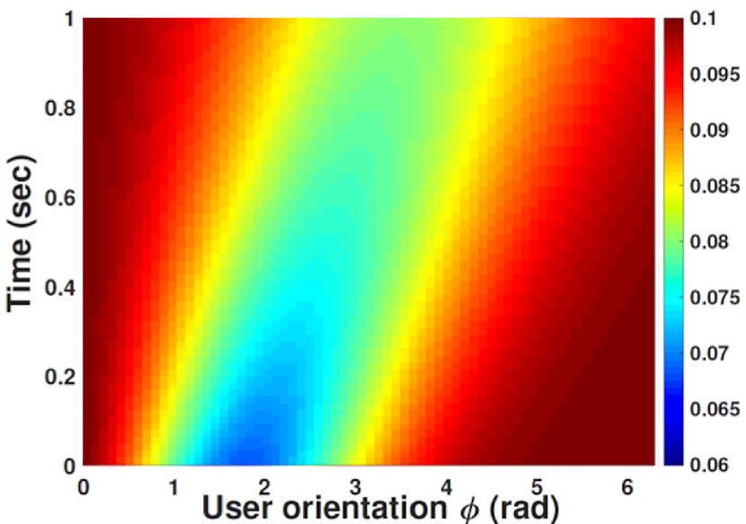
Figure 1: MFE power versus user’s orientation.

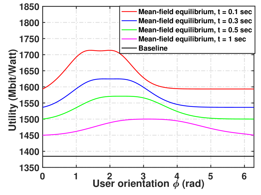
Figure 2: Utility versus user’s orientation.

Fig. 2 shows that, initially, the MFE transmission power decreases as the user orientation approaches $\frac{\pi}{2}$ since the initial distribution is normal with mean $\frac{\pi}{2}$. Thus, the highest proportion of users has an orientation of $\frac{\pi}{2}$, and, thus, users with orientation of $\frac{\pi}{2}$ transmit with the lowest power to reduce interference. As time increases, the distribution of users’ orientation flattens, and, thus, the MFE transmission power decreases for a larger range of orientation. Hence, Fig. 2 shows that the MFE transmission power decreases with the proportion of users’ orientation.

Fig. 2 shows that, at the MFE, the utility decreases with time for all values of the user orientation. This is because, as time increases, the MFE transmission power increases for a larger range of users’ orientations, which increases the interference. Fig. 2 also shows that the MFE achieves higher utility than the baseline. The increase in the utility when using the MFE reaches up to $24\%$ when $\phi=\frac{\pi}{2}$ and $t=0.1$ seconds.

V Conclusion

In this paper, we have proposed a mean-field game to solve the power control problem in ultra-dense millimeter wave network. Our results have quantified the performance gains achieved when using the mean-field approach compared to the baseline in which the nodes transmit with maximum power. Future work will consider applying our framework to more mobile scenarios.

References

- [1] R. Baldemair, T. Irnich, K. Balachandran, E. Dahlman, G. Mildh, Y. Selén, S. Parkvall, M. Meyer, and A. Osseiran “Ultra-dense networks in millimeter-wave frequencies,” IEEE Commun. Mag., vol. 53, no. 1, Jan. 2015.
- [2] O. Semiari, W. Saad, M. Bennis, and B. Maham, "Caching Meets Millimeter Wave Communications for Enhanced Mobility Management in 5G Networks", IEEE Trans. Wirel. Commun., vol. 17, no. 2, pp. 779 - 793, Feb. 2018.
- [3] S. Niknam, B. Natarajan and R. Barazideh, “Interference analysis for finite-area 5G mmWave networks considering blockage effect,” IEEE Access, vol. 6, Apr. 2018.
- [4] Y. Liu, X. Fang, P. Zhou and K. Cheng,“Coalition game for user association and bandwidth allocation in ultra-dense mmWave networks,” in Proc. IEEE Int. Conf. on Commun. in China (ICCC), Qingdao, China, Oct. 2017, pp. 1-5.
- [5] H. Zhang, S. Huang, C. Jiang, K. Long, V. C. M. Leung and H. V. Poor, “Energy efficient user association and power allocation in millimeter-wave-based ultra dense networks With energy harvesting base stations,” IEEE J. Select. Areas Commun., vol. 35, no. 9, pp. 1936-1947, Sep. 2017.
- [6] R. Chen, J. G. Andrews, R. W. Heath and A. Ghosh, “Uplink Power Control in Multi-Cell Spatial Multiplexing Wireless Systems,” IEEE Trans. Wirel. Commun., vol. 6, no. 7, pp. 2700-2711, Jul. 2007.
- [7] N. Abuzainab, W. Saad, C. S. Hong, and H. V. Poor, "Cognitive Hierarchy Theory for Distributed Resource Allocation in the Internet of Things", IEEE Trans. Wirel. Commun., vol. 16, no. 12, pp. 7687 - 7702, Dec. 2017.
- [8] P. Semasinghe and E. Hossain, “Downlink power control in self-organizing dense small cells underlaying macrocells: A mean field game,” IEEE Trans. Mobile Comput., vol. 15, no. 2, pp. 350-363, Feb. 2016.
- [9] M. de Mari, E. Calvanese Strinati, M. Debbah and T. Q. S. Quek, “Joint Stochastic Geometry and Mean Field Game Optimization for Energy-Efficient Proactive Scheduling in Ultra Dense Networks,” IEEE Trans. on Cogn. Commun. Netw., vol. 3, no. 4, pp. 766-781, Dec. 2017.
- [10] T. Bai and R. W. Heath, “Coverage and rate analysis for millimeterwave cellular networks,” IEEE Trans. Wirel. Commun., vol. 14, no. 2, pp. 1100–1114, Feb. 2015.
- [11] S. Rangan, T. Rappaport, and E. Erkip, “Millimeter Wave Cellular Networks: Potentials and Challenges,” Proc. IEEE, vol. 102, no. 3,pp. 366- 385, Mar. 2014.
- [12] V. Petrov, M. Komarov, D. Moltchanov, J. M. Jornet, and Y. Koucheryavy,“Interference and SINR in Millimeter Wave and Terahertz Communication Systems With Blocking and Directional Antennas,” in IEEE Trans. Wirel. Commun., vol. 16, no. 3, pp. 1791-1808, Mar. 2017.
- [13] A. Bensoussan, J. Frehse, and P. Yam, Mean-field games and mean-field type control theory, Springer, 2013.