Convergence Analysis of Gradient-Based Learning with Non-Uniform Learning Rates in Non-Cooperative Multi-Agent Settings

Abstract

Considering a class of gradient-based multi-agent learning algorithms in non-cooperative settings, we provide local convergence guarantees to a neighborhood of a stable local Nash equilibrium. In particular, we consider continuous games where agents learn in (i) deterministic settings with oracle access to their gradient and (ii) stochastic settings with an unbiased estimator of their gradient. Utilizing the minimum and maximum singular values of the game Jacobian, we provide finite-time convergence guarantees in the deterministic case. On the other hand, in the stochastic case, we provide concentration bounds guaranteeing that with high probability agents will converge to a neighborhood of a stable local Nash equilibrium in finite time. Different than other works in this vein, we also study the effects of non-uniform learning rates on the learning dynamics and convergence rates. We find that much like preconditioning in optimization, non-uniform learning rates cause a distortion in the vector field which can, in turn, change the rate of convergence and the shape of the region of attraction. The analysis is supported by numerical examples that illustrate different aspects of the theory. We conclude with discussion of the results and open questions.

1 Introduction

The characterization and computation of equilibria such as Nash equilibria and its refinements constitutes a significant focus in non-cooperative game theory. Several natural questions arises including “how do players find such equilibria?” and “how should the learning process be interpreted?” With these questions in mind, a variety of fields have focused their attention on the problem of learning in games. This has, in turn, lead to a plethora of learning algorithms including gradient play, fictitious play, best response, and multi-agent reinforcement learning among others [13].

From an applications point of view, a more recent trend is in the adoption of game theoretic models of algorithm interaction in machine learning applications. For instance, game theoretic tools are being used to improve the robustness and generalizability of machine learning algorithms; e.g., generative adversarial networks have become a popular topic of study demanding the use of game theoretic ideas to provide performance guarantees [12]. In other work from the learning community, game theoretic concepts are being leveraged to analyze the interaction of learning agents—see, e.g., [15, 21, 3, 33, 23]. Even more recently, convergence analysis to Nash equilibria has been called into question [27]; in its place is a proposal to consider game dynamics as the meaning of the game. This is an interesting perspective as it is well known that in general learning dynamics do not obtain an Nash equilibrium even asymptotically—see, e.g., [14]—and, perhaps more interestingly, many learning dynamics exhibit very interesting limiting behaviors including periodic orbits and chaos—see, e.g., [6, 7, 17, 16].

Despite this activity, we still lack a complete understanding of the dynamics and limiting behaviors of coupled, competing learning algorithms. One may imagine that the myriad results on convergence of gradient descent in optimization readily extend to the game setting. Yet, they do not since gradient-based learning schemes in games do not correspond to gradient flows, a class of flows that are guaranteed to converge to local minimizers almost surely. In particular, the gradient-based learning dynamics for competitive, multi-agent settings have a non-symmetric Jacobian and as a consequence their dynamics may admit complex eigenvalues and non-equilibrium limiting behavior such as periodic orbits. In short, this fact makes it difficult to extend many of the optimization approaches to convergence in single-agent optimization settings to multi-agent settings primarily due to the fact that steps in the direction of individual gradients of players’ costs do not guarantee that each agents cost decreases. In fact, in games, as our examples highlight, a player’s cost can increase when they follow the gradient of their own cost. Counterintuitively, agents can also converge to local maxima of their own costs despite descending their own gradient. These behaviors are due to the coupling between the agents.

Some of the questions that remain unaddressed and to which we provide partial answers include the derivation of error bounds and convergence rates. These are important for ensuring performance guarantees on the collective behavior and can help provide guarantees on subsequent control or incentive policy synthesis. We also investigate the question of how naturally arising features of the learning process for autonomous agents, such as their learning rates, impact the learning path and limiting behavior. This further exposes interesting questions about the overall quality of the limiting behavior and the cost accumulated along the learning path—e.g., is it better to be a slow or fast learner both in terms of the cost of learning and the learned behavior?

Contributions.

We study convergence of a broad class of gradient-based multi-agent learning algorithms in non-cooperative settings by leveraging the framework of $n$-player continuous games along with tools from numerical optimization and dynamical systems theory. We consider a class of learning algorithms

$$x_{i}^{+}=x_{i}-\gamma_{i}g_{i}(x_{i},x_{-i})$$

where $x_{i}$ is the choice variable or action of player $i$, $\gamma_{i}$ is its learning rate, and $g_{i}$ is derived from the gradient of a function that abstractly represents the cost of player $i$. The key feature of non-cooperative settings is coupling of an agent’s cost through all other agents’ choice variables $x_{-i}$.

We consider two settings: (i) agents have oracle access to $g_{i}$ and (ii) agents have an unbiased estimator for $g_{i}$. The class of gradient-based learning algorithms we study encompases a wide variety of approaches to learning in games including multi-agent policy gradient, gradient-based approaches to adversarial learning, and multi-agent gradient-based online optimization. For both the deterministic (oracle gradient access) and the stochastic (unbiased estimators) settings, we provide convergence results for both uniform learning rates—i.e., where $\gamma_{i}=\gamma$ for each player $i\in\{1,\ldots,n\}$—and for non-uniform learning rates. The latter of which arises more naturally in the study of the limiting behavior of autonomous learning agents.

In the deterministic setting, we derive asymptotic and finite-time convergence rates for the coupled learning processes to a refinement of local Nash equilibria known as differential Nash equilibria [28] (a class of equilibria that are generic amongst local Nash equilibria). In the stochastic setting, leveraging the results of stochastic approximation and dynamical systems, we derive asymptotic convergence guarantees to stable local Nash equilibria as well as high-probability, finite-time guarantees for convergence to a neighborhood of a Nash equilibrium. The analytical results are supported by several illustrative numerical examples. We also provide discussion on the effect of non-uniform learning rates on the learning path—that is, different learning rates warp the vector field dynamics. Coordinate based learning rates are typically leveraged in gradient-based optimization schemes to speed up convergence or avoid poor quality local minima. In games, however, the interpretation is slightly different since each of the coordinates of the dynamics corresponds to minimizing a different cost function along the respective coordinate axis. The resultant effect is a distortion of the vector field in such a way that it has the effect of leading the joint action to a point which has a lower value for the slower player relative to the flow of the dynamics given a uniform learning rate and the same initialization. In this sense, it seems that the answer to the question posed above is that it is most beneficial for an agent to have the slower learning rate.

Organization.

The remainder of the paper is organized as follows. We start with mathematical and game-theoretic preliminaries in Section 2 which is followed by the main convergence results for the deterministic setting (Section 3) and the stochastic setting (Section 4). Within each of the latter two sections, we present convergence results for both the case where agents have uniform and non-uniform learning rates. In Section 5, we present several numerical examples which help to illustrate the theoretical results and also highlight some directions for future inquiry. Finally, we conclude with discussion and future work in Section 6.

2 Preliminaries

Consider a setting in which at iteration $k$, each agent $i\in\mathcal{I}=\{1,\ldots,n\}$ updates their choice variable $x_{i}\in X_{i}=\mathbb{R}^{d_{i}}$ by the process

$$x_{i,k+1} =x_{i,k}-\gamma_{i,k}g_{i}(x_{i,k},x_{-i,k}).$$ (1)

where $\gamma_{i}$ is agent $i$’s learning rate, $x_{-i}=(x_{j})_{j\in\mathcal{I}/\{i\}}\in\prod_{j\in\mathcal{I}/\{i\}}X_{j}$ denotes the choices of all agents excluding the $i$-th agent, and $(x_{i},x_{-i})\in X=\prod_{i\in\mathcal{I}}X_{i}$. Within the above setting, the class of learning algorithms we consider is such that for each $i\in\mathcal{I}$, there exists a sufficiently smooth function $f_{i}\in C^{q}(X,\mathbb{R})$, $q\geq 2$ such that $g_{i}$ is either $D_{i}f_{i}$, where $D_{i}(\cdot)$ denotes the derivative with respect to $x_{i}$, or an unbiased estimator of $D_{i}f_{i}$—i.e., $g_{i}\equiv\widehat{D_{i}f_{i}}$ where $\mathbb{E}[\widehat{D_{i}f_{i}}]=D_{i}f_{i}$.

The collection of costs $(f_{1},\ldots,f_{n})$ on $X=X_{1}\times\cdots\times X_{n}$ where $f_{i}:X\rightarrow\mathbb{R}$ is agent $i$’s cost function and $X_{i}=\mathbb{R}^{d_{i}}$ is their action space defines a continuous game. In this continuous game abstraction, each player $i\in\mathcal{I}$ aims to selection an action $x_{i}\in X_{i}$ that minimizes their cost $f_{i}(x_{i},x_{-i})$ given the actions of all other agents, $x_{-i}\in X_{-i}$. That is, players myopically update their actions by following the gradient of their cost with respect to their own choice variable. For a symmetric matrix $A\in\mathbb{R}^{d\times d}$, let $\lambda_{d}(A)\leq\cdots\leq\lambda_{1}(A)$ be its eigenvalues. For a matrix $A\in\mathbb{R}^{d\times d}$, let $\mathrm{spec}(A)=\{\lambda_{j}(A)\}$ be the spectrum of $A$.

Assumption 1.

For each $i\in\mathcal{I}$, $f_{i}\in C^{r}(X,\mathbb{R})$ for $r\geq 2$ and $\omega(x)\equiv(D_{1}f_{1}(x)\ \cdots\ D_{n}f_{n}(x))$ is $L$–Lipschitz.

Let $D_{i}^{2}f_{i}$ denote the second partial derivative of $f_{i}$ with respect to $x_{i}$ and $D_{ji}f_{i}$ denote the partial derivative of $D_{i}f_{i}$ with respect to $x_{j}$. The game Jacobian—i.e., the Jacobian of $\omega$—is given by

$$J(x)=\begin{bmatrix}D_{1}^{2}f_{1}(x)&\cdots&D_{1n}f_{1}(x)\\ \vdots&\ddots&\vdots\\ D_{n1}f_{n}(x)&\cdots&D_{n}^{2}f_{n}(x)\end{bmatrix}.$$

The entries of the above matrix are dependent on $x$, however, we drop this dependence where obvious. Note that each $D_{i}^{2}f_{i}$ is symmetric under Assumption 1, yet $J$ is not. This is an important point and causes the subsequent analysis to deviate from the typical analysis of (stochastic) gradient descent.

The most common characterization of limiting behavior in games is that of a Nash equilibrium. The following definitions are useful for our analysis.

Definition 1.

A strategy $x\in X$ is a local Nash equilibrium for the game $(f_{1},\ldots,f_{n})$ if for each $i\in\mathcal{I}$ there exists an open set $W_{i}\subset X_{i}$ such that $x_{i}\in W_{i}$ and $f_{i}(x_{i},x_{-i})\leq f_{i}(x_{i}^{\prime},x_{-i})$ for all $x_{i}^{\prime}\in W_{i}$. If the above inequalities are strict, $x$ is a strict local Nash equilibrium.

Definition 2.

A point $x\in X$ is said to be a critical point for the game if $\omega(x)=0$.

We denote the set of critical points as $\mathcal{C}=\{x\in X|\ \omega(x)=0\}$. Analogous to single-player optimization settings, for each player, viewing all other players’ actions as fixed, there are necessary and sufficient conditions which characterize local optimality.

Proposition 1 ([28]).

If $x$ is a local Nash equilibrium of the game $(f_{1},\ldots,f_{n})$, then $\omega(x)=0$ and $D_{i}^{2}f_{i}(x)\geq 0$. On the other hand, if $\omega(x)=0$ and $D_{i}^{2}f_{i}(x)>0$, then $x\in X$ is a local Nash equilibrium.

The sufficient conditions in the above result give rise to the following definition of a differential Nash equilibrium.

Definition 3 ([28]).

A strategy $x\in X$ is a differential Nash equilibrium if $\omega(x)=0$ and $D^{2}_{i}f_{i}(x)>0$ for each $i\in\mathcal{I}$.

Differential Nash need not be isolated. However, if $J(x)$ is non-degenerate—meaning that $\det J(x)\neq 0$—for a differential Nash $x$, then $x$ is an isolated strict local Nash equilibrium. Non-degenerate differential Nash are generic amongst local Nash equilibria and they are structurally stable [29] which ensures they persist under small perturbations. This result also implies an asymptotic convergence result: if the spectrum of $J$ is strictly in the right-half plane (i.e. $\mathrm{spec}(J(x))\subset\mathbb{C}_{+}^{\circ}$), then a differential Nash equilibrium $x$ is (exponentially) attracting under the flow of $-\omega$ [28, Proposition 2]. We say such equilibria are stable.

3 Deterministic Setting

The multi-agent learning framework we analyze is such that each agent’s rule for updating their choice variable consists of the agent modifying their action $x_{i}$ in the direction of their individual gradient $D_{i}f_{i}$. Let us first consider the setting in which each agent $i$ has oracle access to $g_{i}$. The learning dynamics are given by

$$x_{k+1}=x_{k}-\Gamma\omega(x_{k})$$ (2)

where $\Gamma=\mathrm{blockdiag}(\gamma_{1}I_{d_{1}},\ldots,\gamma_{n}I_{d_{n}})$ with $I_{d_{i}}$ denoting the $d_{i}\times d_{i}$ identity matrix. Within this setting we consider both the cases where the agents have a constant uniform learning rate—i.e., $\gamma_{i}\equiv\gamma$—and where their learning rates are non-uniform, but constant—i.e., $\gamma_{i}$ is not necessarily equal to $\gamma_{j}$ for any $i,j\in\mathcal{I}$, $j\neq i$.

Let $S(x)=\frac{1}{2}(J(x)+J(x)^{T})$ be the symmetric part of $J(x)$. Define

$$\alpha=\min_{x\in B_{r}(x^{\ast})}\lambda_{d}\big{(}S(x)^{T}S(x)\big{)}$$

and

$$\beta=\max_{x\in B_{r}(x^{\ast})}\lambda_{1}(J(x)^{T}J(x))$$

where $B_{r}(x^{\ast})$ is a $r$–radius ball around $x^{\ast}$. For a stable differential Nash $x^{\ast}$, let $B_{r}(x^{\ast})$ be a ball of radius $r>0$ around the equilibrium $x^{\ast}$ that is contained in the region of attraction $\mathcal{V}(x^{\ast})$ for $x^{\ast}$. Let $B_{r_{0}}(x^{\ast})$ with $0<r_{0}<\infty$ be the largest ball contained in the region of attraction of $x^{\ast}$.

3.1 Uniform Learning Rates

With $\gamma_{i}=\gamma$ for each $i\in\mathcal{I}$, the learning rule (2) can be thought of as a discretized numerical scheme approximating the continuous time dynamics

$$\dot{x}=-\omega(x).$$

With a judicious choice of learning rate $\gamma$, (2) will converge (at an exponential rate) to a locally stable equilibrium of the dynamics.

Proposition 2.

Consider an $n$–player continuous game $(f_{1},\ldots,f_{n})$ satisfying Assumption 1. Let $x^{\ast}\in X$ be a stable differential Nash equilibrium. Suppose agents use the gradient-based learning rule $x_{k+1}=x_{k}-\gamma\omega(x_{k})$ with learning rates $0<\gamma<\tilde{\gamma}$ where $\tilde{\gamma}$ is the smallest positive $h$ such that $\max_{j}|1-h\lambda_{j}(J(x^{\ast}))|=1$. Then, for $x_{0}\in B_{r}(x^{\ast})\subset\mathcal{V}(x^{\ast})$, $x_{k}\rightarrow x^{\ast}$ exponentially.

The above result provides a range for the possible learning rates for which (2) converges to a stable differential Nash equilibrium $x^{\ast}$ of $(f_{1},\ldots,f_{n})$ assuming agents initialize in a ball contained in the region of attraction of $x^{\ast}$. Note that the usual assumption in gradient-based approaches to single-objective optimization problems (in which case $J$ is symmetric) is that $\gamma<1/L$, where objective being minimized is $L$-Lipschitz. This is sufficient to guarantee convergence since the spectral radius of a matrix is always less than any operator norm which, in turn, ensures that $|1-\gamma\lambda_{j}|<1$ for each $\lambda_{j}\in\mathrm{spec}(J(x^{\ast}))$. If the game is a potential game—i.e., there exists a function $\phi$ such that $D_{i}f_{i}=D_{i}\phi$ for each $i$ which occurs if and only if $D_{ij}f_{i}=D_{ji}f_{j}$—then convergence analysis coincides with gradient descent so that any $\gamma<1/L$ where $L$ is the Lipschitz constant of $\omega$ results in local asymptotic convergence.

The convergence guarantee in Proposition 2 is asymptotic in nature. It is often useful, from both an analysis and synthesis perspective, to have non-asymptotic or finite-time convergence results. Such results can be used to provide guarantees on decision-making processes wrapped around the coupled learning processes of the otherwise autonomous agents. The next result, provides a finite-time convergence guarantee for gradient-based learning where agents uniformly use a fixed step size.

Let $B_{r}(x^{\ast})$ be defined as before with the added condition that it be defined to be the largest ball in the region of attraction such that on $B_{r}(x^{\ast})$ the symmetric part of $J$—i.e., $S\equiv\frac{1}{2}(J+J^{T})$—is positive definite.

Theorem 1.

Consider a game $(f_{1},\ldots,f_{n})$ on $X=X_{1}\times\cdots\times X_{n}$ satisfying Assumption 1. Let $x^{\ast}\in X$ be a stable differential Nash equilibrium. Suppose $x_{0}\in B_{r}(x^{\ast})$ and that $\alpha<\beta$. Then, given $\varepsilon>0$, the gradient-based learning dynamics with learning rate $\gamma=\sqrt{\alpha}/\beta$ obtains an $\varepsilon$–differential Nash such that $x_{k}\in B_{\varepsilon}(x^{\ast})\subset B_{r}(x^{\ast})$ for all

$$k\geq\left\lceil 2\frac{\beta}{\alpha}\log\frac{r}{\varepsilon}\right\rceil.$$

Before we proceed to the proof, let us remark on the assumption that $\alpha<\beta$. First, $\alpha\leq\beta$ is always true; indeed, suppressing the dependence on $x$,

$$\lambda_{d}(S^{T}S)\textstyle\leq\lambda_{1}(S^{T}S) \textstyle\leq\sigma_{\max}(J)^{2}=\lambda_{1}(J^{T}J)$$

where $\sigma_{\max}(\cdot)$ denotes the largest singular value of its argument. Thus, the condition that $\alpha<\beta$ is generally true; for equality to hold, the symmetric part of $J(x)$ would have repeated eigenvalues, which is not generic. Hence, we include this assumption in Theorem 1, but note that it is not restrictive and is fairly benign.

• First, note that $\|x_{k+1}-x^{\ast}\|=\|\tilde{g}(x_{k})-\tilde{g}(x^{\ast})\|$ where $\tilde{g}(x)=x-\gamma\omega(x)$. Now, given $x_{0}\in B_{r}(x^{\ast})$, by the mean value theorem,

  $$\textstyle\|\tilde{g}(x_{0})-\tilde{g}(x^{\ast})\|=\|\int_{0}^{1}D\tilde{g}(\tau x_{0}+(1-\tau)x^{\ast})(x_{0}-x^{\ast})d\tau\|\leq\sup_{x\in B_{r}(x^{\ast})}\|D\tilde{g}(x)\|\|x_{0}-x^{\ast}\|.$$

  Hence, it suffices to show that for the choice of $\gamma$, the eigenvalues of $I-\gamma J(x)$ are in the unit circle. Indeed, since $\omega(x^{\ast})=0$, we have that

  $$\textstyle\|x_{k+1}-x^{\ast}\|_{2} =\|x_{k}-x^{\ast}-\gamma(\omega(x_{k})-\omega(x^{\ast}))\|_{2}\textstyle\leq\sup_{x\in B_{r}(x^{\ast})}\|I-\gamma J(x)\|_{2}\|x_{k}-x^{\ast}\|_{2}$$

  If $\sup_{x\in B_{r}(x^{\ast})}\|I-\gamma J(x)\|_{2}$ is less than one, then the dynamics are contracting. For notational convenience, we drop the explicit dependence on $x$. Since $\lambda_{d}(S)\geq\sqrt{\alpha}$ on $B_{r}(x^{\ast})$,

  $$(I-\gamma J)^{T} (I-\gamma J)\leq(1-2\gamma\lambda_{d}(S)+\gamma^{2}\lambda_{1}(J^{T}J))I\leq\textstyle(1-\frac{\alpha}{\beta})I$$

  where the last inequality holds for $\gamma=\sqrt{\alpha}/{\beta}$. Hence,

  $$\textstyle\|x_{k+1}-x^{\ast}\|_{2} \textstyle\leq\sup_{x\in B_{r}(x^{\ast})}\|I-\gamma J(x)\|_{2}\|x_{k}-x^{\ast}\|_{2}\leq\textstyle(1-\frac{\alpha}{\beta})^{1/2}\|x_{k}-x^{\ast}\|_{2}.$$

  Since $\alpha<\beta$, we have that $(1-\alpha/\beta)<\exp(-\alpha/\beta)$ so that

  $$\|x_{T}-x^{\ast}\|_{2}\leq\exp(-T\alpha/(2\beta))\|x_{0}-x^{\ast}\|_{2}.$$

  This, in turn, implies that $x_{k}\in B_{\varepsilon}(x^{\ast})$ for all $k\geq T=\lceil 2\frac{\beta}{\alpha}\log(r/\varepsilon)\rceil$. ∎

Note that $\gamma=\sqrt{\alpha}/{\beta}$ is selected to minimize $1-2\gamma\lambda_{1}(S)+\gamma^{2}\lambda_{d}(J^{T}J)$. Hence, this is the fastest learning rate given the worst case eigenstructure of $J$ over the ball $B_{r}(x^{\ast})$ for the choice of operator norm $\|\cdot\|_{2}$. We note, however, that faster convergence is possible as indicated by Proposition 2 and observed in the examples in Section 5. Indeed, we note that the spectral radius $\rho(\cdot)$ of a matrix is always less than its maximum singular value—i.e. $\rho(I-\gamma J)\leq\|I-\gamma J\|_{2}$—so it is possible to contract at a faster rate. We remark that if $J$ was symmetric (i.e., in the case of a potential game [24] or a single-agent optimization problem), then $\rho(I-\gamma J)=\|I-\gamma J\|_{2}$. In games, however, $J$ is not symmetric.

3.2 Non-Uniform Learning Rates

Let us now consider the case when agents have their own individual learning rate $\gamma_{i}$, yet still have oracle access to their individual gradients. This is, of course, more natural in the study of autonomous learning agents as opposed to efforts for computing Nash equilibria for a given game.

Proposition 3.

Consider an $n$–player game $(f_{1},\ldots,f_{n})$ satisfying Assumption 1. Let $x^{\ast}\in X$ be a stable differential Nash equilibrium. Suppose agents use the gradient-based learning rule $x_{k+1}=x_{k}-\Gamma\omega(x_{k})$ with learning rates $\gamma_{i}$ such that $\rho(I-\Gamma J(x))<1$ for all $x\in\mathcal{V}(x^{\ast})$. Then, for $x_{0}\in\mathcal{V}(x^{\ast})$, $x_{k}\rightarrow x^{\ast}$ exponentially.

The proof is a direct application of Ostrowski’s theorem [26]. We provide a simple proof via Lyapunov argument for posterity.

Mazumdar and Ratliff [21] show that (2) will almost surely avoid strict saddle points of the dynamics, some of which are Nash equilibria in non-zero sum games. Note that the set of critical points $\mathcal{C}$ contains more than just the local Nash equilibria. Hence, except on a set of measure zero, (2) will converge to a stable attractor of $\dot{x}=-\omega(x)$ which includes stable limit cycles and stable local non-Nash critical points.

Letting $\tilde{g}(x)=x-\Gamma\omega(x)$, since $\omega\in C^{q}$ for some $q\geq 1$, $\tilde{g}\in C^{q}$, the expansion

$$\tilde{g}(x)=\tilde{g}(x^{\ast})+(I-\Gamma J(x))(x-x^{\ast})+R(x-x^{\ast})$$

holds, where $R$ satisfies $\lim_{x\rightarrow x^{\ast}}\|R(x-x^{\ast})\|/\|x-x^{\ast}\|=0$ so that given $c>0$, there exists an $r>0$ such that $\|R(x-x^{\ast})\|\leq c\|x-x^{\ast}\|$ for all $x\in B_{r}(x^{\ast})$.

Proposition 4.

Suppose that $\|I-\Gamma J(x)\|<1$ for all $x\in B_{r_{0}}(x^{\ast})\subset\mathcal{V}(x^{\ast})$ so that there exists $r^{\prime},r^{\prime\prime}$ such that $\|I-\Gamma J(x)\|\leq r^{\prime}<r^{\prime\prime}<1$ for all $x\in B_{r_{0}}(x^{\ast})$. For $1-r^{\prime\prime}>0$, let $0<r<\infty$ be the largest $r$ such that $\|R(x-x^{\ast})\|\leq(1-r^{\prime\prime})\|x-x^{\ast}\|$ for all $x\in B_{r}(x^{\ast})$. Furthermore, let $x_{0}\in B_{r^{\ast}}(x^{\ast})$, where $r^{\ast}=\min\{r,r_{0}\}$, be arbitrary. Then, given $\varepsilon>0$, gradient-based learning with learning rates $\Gamma$ obtains an $\varepsilon$–differential Nash equilibrium in finite time—i.e., $x_{k}\in B_{\varepsilon}(x^{\ast})$ for all $k\geq T=\lceil\frac{1}{\delta}\log\left(r^{\ast}/\varepsilon\right)\rceil$ where $\delta=r^{\prime\prime}-r^{\prime}$.

The proof follows the proof of Theorem 1 in [2] with a few minor modifications; we provide it in Appendix A.1 for completeness.

Remark 1.

We note that the proposition can be more generally stated with the assumption that $\rho(I-\Gamma J(x))<1$, in which case there exists some $\delta$ defined in terms of bounds on powers of $I-\Gamma J$. We provide the proof of this in Appendix A.1. We also note that these results hold even if $\Gamma$ is not a diagonal matrix as we have assumed as long as $\rho(I-\Gamma J(x))<1$.

A perhaps more interpretable finite bound stated in terms of the game structure can also be obtained. Consider the case in which players adopt learning rates $\gamma_{i}=\sqrt{\alpha}/(\beta k_{i})$ with $k_{i}\geq 1$. Given a stable differential Nash equilibrium $x^{\ast}$, let $B_{r}(x^{\ast})$ be the largest ball of radius $r$ contained in the region of attraction on which $\tilde{S}\equiv\frac{1}{2}(\tilde{J}^{T}+\tilde{J})$ is positive definite where $\tilde{\omega}=(D_{i}f_{i}/k_{i})_{i\in\mathcal{I}}$ so that $\tilde{J}\equiv D\tilde{\omega}$, and define

$$\tilde{\alpha}=\textstyle\min_{x\in B_{r}(x^{\ast})}\lambda_{d}\big{(}\tilde{S}(x)^{T}\tilde{S}(x)\big{)}$$

and

$$\textstyle\tilde{\beta}=\max_{x\in B_{r}(x^{\ast})}\lambda_{1}(\tilde{J}(x)^{T}\tilde{J}(x)).$$

Given a stable differential Nash equilibrium $x^{\ast}$, let $B_{r}(x^{\ast})$ be the largest ball contained in the region of attraction $\mathcal{V}(x^{\ast})$ on which $S^{T}S$ is positive definite—i.e., $\sqrt{\alpha}>0$.

Theorem 2.

Suppose that Assumption 1 holds and that $x^{\ast}\in X$ is a stable differential Nash equilibrium. Let $x_{0}\in B_{r}(x^{\ast})$, $\alpha<k_{\min}\beta$, $\sqrt{\alpha}/k_{\min}\leq\sqrt{\tilde{\alpha}}$, and for each $i$, $\gamma_{i}=\sqrt{\alpha}/(\beta k_{i})$ with $k_{i}\geq 1$. Then, given $\varepsilon>0$, the gradient-based learning dynamics with learning rates $\gamma_{i}$ obtain an $\varepsilon$–differential Nash such that $x_{k}\in B_{\varepsilon}(x^{\ast})$ for all

$$k\geq\left\lceil 2\frac{\beta k_{\min}}{{\alpha}}\log\left(\frac{r}{\varepsilon}\right)\right\rceil.$$

• First, note that $\|x_{k+1}-x^{\ast}\|=\|\tilde{g}(x_{k})-\tilde{g}(x^{\ast})\|$ where $\tilde{g}(x)=x-\Gamma\omega(x)$. Now, given $x_{0}\in B_{r}(x^{\ast})$, by the mean value theorem,

  $$\textstyle\|\tilde{g}(x_{0})-\tilde{g}(x^{\ast})\|=\|\int_{0}^{1}D\tilde{g}(\tau x_{0}+(1-\tau)x^{\ast})(x_{0}-x^{\ast})d\tau\|\leq\sup_{x\in B_{r}(x^{\ast})}\|D\tilde{g}(x)\|\|x_{0}-x^{\ast}\|.$$

  Hence, it suffices to show that for the choice of $\Gamma$, the eigenvalues of $I-\Gamma J(x)$ live in the unit circle. Then an inductive argument can be made with the inductive hypothesis that $x_{k}\in B_{r}(x^{\ast})$. Let $\Lambda=\mathrm{diag}\left(1/k_{1},\ldots,1/k_{n}\right)$. Then we need to show that $I-\gamma\Lambda J$ has eigenvalues in the unit circle. Since $\omega(x^{\ast})=0$, we have that

  $$\|x_{k+1}-x^{\ast}\|_{2}=\|x_{k}-x^{\ast}-\gamma\Lambda(\omega(x_{k})-\omega(x^{\ast}))\|_{2}\leq\textstyle\sup_{x\in B_{r}(x^{\ast})}\|I-\gamma\Lambda J(x)\|_{2}\|x_{k}-x^{\ast}\|_{2}.$$

  If $\sup_{x\in B_{r}(x^{\ast})}\|I-\gamma\Lambda J(x)\|_{2}$ is less than one, where the norm is the operator $2$–norm, then the dynamics are contracting. For notational convenience, we drop the explicit dependence on $x$. Then,

  $$(I-\gamma\Lambda J)^{T}(I-\gamma\Lambda J)\leq\textstyle(1-2\gamma\lambda_{d}(\tilde{S})+\frac{\gamma^{2}\lambda_{1}(J^{T}J)}{k_{\min}^{2}})I\textstyle \leq(1-2\gamma\sqrt{\alpha}/k_{\min}+\alpha/(\beta k_{\min}))I$$

  $$\textstyle=(1-\alpha/(\beta k_{\min}))I.$$

  The first inequality holds since $\lambda_{1}(J^{T}J/k_{\min}^{2})\geq\lambda_{1}(J^{T}\Lambda^{2}J)$. Indeed, first observe that the singular values of $\Lambda J^{T}J\Lambda$ are the same as those of $J^{T}\Lambda^{2}J$ since the latter is positive definite symmetric. Thus, by noting that $\|A\|_{2}=\sigma_{\max}(A)$ and employing Cauchy-Schwartz, we get that $\|\Lambda\|_{2}^{2}\|J^{T}J\|_{2}\geq\|\Lambda J^{T}J\Lambda\|_{2}$ and hence, the inequality.

Using the above to bound $\sup_{x\in B_{r}(x^{\ast})}\|I-\gamma\Lambda J(x)\|_{2}$, we have $\|x_{k+1}-x^{\ast}\|_{2}\leq\textstyle(1-\frac{\alpha}{\beta k_{\min}})^{1/2}\|x_{k}-x^{\ast}\|_{2}$. Since $\alpha<k_{\min}\beta$, $(1-\alpha/(\beta k_{\min}))<e^{-\alpha/(\beta k_{\min})}$ so that $\|x_{k+1}-x^{\ast}\|_{2}\leq e^{-T\alpha/(2k_{\min}\beta)}\|x_{0}-x^{\ast}\|_{2}$. This, in turn, implies that $x_{k}\in B_{\varepsilon}(x^{\ast})$ for all $k\geq T=\lceil 2\frac{\beta k_{\min}}{\alpha}\log(r/\varepsilon)\rceil$.

∎

Multiple learning rates lead to a scaling rows which can have a significant effect on the eigenstructure of the matrix, thereby making the relationship between $\Gamma J$ and $J$ difficult to reason about. None-the-less, there are numerous approaches to solving nonlinear systems of equations (or differential equations expressed as a set of nonlinear system of equations) that employ preconditioning (i.e., coordinate scaling). The purpose of using a preconditioning matrix is to rescale the problem and achieve better or faster convergence. Many of these results directly translate to convergence guarantees for learning in games when the learning rates are not uniform; however, in the case of understanding convergence properties for autonomous agents learning an equilibrium—as opposed to computing an equilibrium—the preconditioner is not subject to design. Perhaps this reveals an interesting direction of future research in terms of synthesizing games or learning rules via incentivization or otherwise exogenous control policies for either coordinating agents or improving the learning process—e.g., using incentives to induce a particular equilibrium while also encouraging faster learning.

4 Stochastic Setting

In this section, we consider gradient-based learning rules for each agent where the agent does not have oracle access to their individual gradients, but rather has an unbiased estimator in its place. In particular, for each player $i\in\mathcal{I}$, consider the noisy gradient-based learning rule given by

$$x_{i,k+1}=x_{i,k}-\gamma_{i,k}(\omega(x_{k})+w_{i,k+1})$$ (3)

where $\gamma_{i,k}$ is the learning rate and $w_{i,k}$ is an independent identically distributed stochastic process. In order to prove a high-probability, finite sample convergence rate, we can leverage recent results for convergence of nonlinear stochastic approximation algorithms. The key is in formulating the the learning rule for the agents and in leveraging the notion of a stable differential Nash equilibrium which has analogous properties as a locally stable equilibrium for a nonlinear dynamical system. Making the link between the discrete time learning update and the limiting continuous time differential equation and its equilibria allows us to draw on rich existing convergence analysis tools.

In the first part of this section, we provide convergence rate results for the case where the agents use a uniform learning rate—i.e. $\gamma_{i,k}\equiv\gamma_{k}$. In the second part of this section, we extend these results to the case where agents use non-uniform learning rates—that is, each agent has its own learning rate $\gamma_{i,k}$—by incorporating some additional assumptions and leveraging two-timescale analysis techniques from dynamical systems theory.

We require some modified assumptions in this section on the learning process structure.

Assumption 2.

The gradient-based learning rule (3) satisfies the following:

1. Given the filtration $\mathcal{F}_{k}=\sigma(x_{s},w_{1,s},w_{2,s},s\leq k)$, $\{w_{i,k+1}\}_{i\in\mathcal{I}}$ are conditionally independent. Moreovoer, for each $i\in\mathcal{I}$, $\mathbb{E}[w_{i,k+1}|\ \mathcal{F}_{k}]=0$ almost surely (a.s.), and $\mathbb{E}[\|w_{i,k+1}\||\ \mathcal{F}_{k}]\leq c_{i}(1+\|x_{k}\|)$ a.s. for some constants $c_{i}\geq 0$.

2. For each $i\in\mathcal{I}$, the stepsize sequence $\{\gamma_{i,k}\}_{k}$ contain positive scalars such that

   1. $\sum_{i}\sum_{k}\gamma_{i,k}^{2}<\infty$;

   2. $\sum_{k}\gamma_{i,k}=\infty$;

   3. and, $\gamma_{2,k}=o(\gamma_{1,k})$.

3. Each $f_{i}\in C^{q}(\mathbb{R}^{d},\mathbb{R})$ for some $q\geq 3$ and each $f_{i}$ and $\omega$ are $L_{i}$– and $L_{\omega}$–Lipschitz, respectively.

4.1 Uniform Learning Rates

Before concluding, we specialize to the case in which agents have the same learning rate sequence $\gamma_{i,k}=\gamma_{k}$ for each $i\in\mathcal{I}$.

Theorem 3.

Suppose that $x^{\ast}$ is a stable differential Nash equilibrium of the game $(f_{1},\ldots,f_{n})$ and that Assumption 2 holds (excluding A2b.iii). For each $k$, let $k_{0}\geq 0$ and

$$\textstyle\zeta_{k}=\max_{k_{0}\leq s\leq k-1}\big{(}\exp(-\lambda\sum_{\ell=s+1}^{k-1}\gamma_{\ell}\big{)}\gamma_{s}.$$

Fix any $\varepsilon>0$ such that $B_{\varepsilon}(x^{\ast})\subset B_{r}(x^{\ast})\subset\mathcal{V}$ where $\mathcal{V}$ is the region of attraction of $x^{\ast}$. There exists constants $C_{1},C_{2}>0$ and functions $h_{1}(\varepsilon)=O(\log(1/\varepsilon))$ and $h_{2}(\varepsilon)=O(1/\varepsilon)$ so that whenever $T\geq h_{1}(\varepsilon)$ and $k_{0}\geq N$, where $N$ is such that $1/\gamma_{k}\geq h_{2}(\varepsilon)$ for all $k\geq N$, the samples generated by the gradient-based learning rule satisfy

$$\textstyle\Pr\left(\bar{x}(t)\in B_{\varepsilon}(x^{\ast})\ \forall t\geq t_{k_{0}}+T+1|\ \bar{x}(t_{k_{0}})\in B_{r}(x^{\ast})\right)$$

$$\qquad\textstyle\geq 1-\sum_{s=k_{0}}^{\infty}\big{(}C_{1}\exp(-C_{2}\varepsilon^{1/2}/\gamma_{s}^{1/2})\textstyle+C_{1}\exp(-C_{2}\min\{\varepsilon,\varepsilon^{2}\}/\zeta_{s})\big{)}$$

where the constants depend only on parameters $\lambda,r,\tau_{L}$ and the dimension $d=\sum_{i}d_{i}$. Then stochastic gradient-based learning in games obtains an $\varepsilon$–stable differential Nash $x^{\ast}$ in finite time with high probability.

The above theorem implies that $x_{k}\in B_{\varepsilon}(x^{\ast})$ for all $k\geq k_{0}+\lceil\log(4\tilde{K}/\varepsilon)\lambda^{-1}\rceil+1$ with high probability for some constant $\tilde{K}$ that depends only on $\lambda,r,\tau_{L}$, and $d$.

• Since $x^{\ast}$ is a stable differential Nash equilibrium, $J(x^{\ast})$ is positive definite and $D_{i}^{2}f_{i}(x^{\ast})$ is positive definite for each $i\in\mathcal{I}$. Thus $x^{\ast}$ is a locally asymptotically stable hyperbolic equilibrium point of $\dot{x}=-\omega(x)$. Hence, the assumptions of Theorem 1.1 [32] are satisfied so that we can invoke the result which gives us the high probability bound for stochastic gradient-based learning in games. ∎

The above theorem has a direct corollary specializing to the case where the gradient-based learning rule with uniform stepsizes is initialized inside a ball of radius $r$ constained in the region of attraction—i.e., $B_{r}(x^{\ast})\subset\mathcal{V}$.

Corollary 1.

Let $x^{\ast}$ be a stable differential Nash equilibrium of $(f_{1},\ldots,f_{n})$ and suppose that Assumption 2 holds (excluding A2b.iii). Fix any $\varepsilon>0$ such that $B_{\varepsilon}(x^{\ast})\subset B_{r}(x^{\ast})\subset\mathcal{V}$. Let $\zeta_{k}$, $T$, and $h_{2}(\varepsilon)$ be defined as in Theorem 3. Suppose that $1/\gamma_{k}\geq h_{2}(\varepsilon)$ for all $k\geq 0$ and that $x_{0}\in B_{r}(x^{\ast})$. Then, with $C_{1},C_{2}>0$ as in Theorem 3,

$$\textstyle\Pr\left(\bar{x}(t)\in B_{\varepsilon}(x^{\ast})\ \forall t\geq T+1|\ \bar{x}(t_{k_{0}})\in B_{r}(x^{\ast})\right)$$

$$\qquad\textstyle\geq 1-\sum_{s=0}^{\infty}\big{(}C_{1}\exp(-C_{2}\varepsilon^{1/2}/\gamma_{s}^{1/2})\textstyle+C_{1}\exp(-C_{2}\min\{\varepsilon,\varepsilon^{2}\}/\zeta_{s})\big{)}.$$

4.2 Non-Uniform Learning Rates

Consider now that agents have their own learning rates $\gamma_{i,k}$ for each $i\in\mathcal{I}$. In environments with several autonomous agents, as compared to the objective of computing Nash equilibria in a game, it is perhaps more reasonable to consider the scenario in which the agents have their own individual learning rate. For the sake of brevity, we show the convergence result in detail for the two agent case—that is, where $\mathcal{I}=\{1,2\}$. We note that the extension to $n$ agents is straightforward. The proof leverages recent results from the theory of stochastic approximation presented in [9] and we note that our objective here is to show that they apply to games and provide commentary on the interpretation of the results in this context.

The gradient-based learning rules are given by

$$x_{i,k+1}=x_{i,k}-\gamma_{i,k}(\omega(x_{k})+w_{i,k+1})$$ (4)

so that with $\gamma_{2,k}=o(\gamma_{1,k})$, in the limit $\tau\rightarrow 0$, the above system can be thought of as approximating the singularly perturbed system

$$\begin{bmatrix}\dot{x}_{1}(t)\\ \dot{x}_{2}(t)\end{bmatrix}=-\begin{bmatrix}D_{1}f_{1}(x_{1}(t),x_{2}(t))\\ \tau D_{2}f_{2}(x_{1}(t),x_{2}(t))\end{bmatrix}$$ (5)

Indeed, since $\lim_{k\rightarrow\infty}\gamma_{2,k}/\gamma_{1,k}\rightarrow 0$—i.e., $\gamma_{2,k}\rightarrow 0$ at a faster rate than $\gamma_{1,k}$—updates to $x_{1}$ appear to be equilibriated for the current quasi-static $x_{2}$ as the dynamics in (5) suggest.

4.2.1 Asymptotic Convergence in the Non-Uniform Learning Rate Setting

Assumption 3.

For fixed $x_{2}\in X_{2}$, the system $\dot{x}_{1}(t)=-D_{1}f_{1}(x_{1}(t),x_{2})$ has a globally asymptotically stable equilibrium $\lambda(x_{2})$.

Lemma 1.

Under Assumptions 2 and 3, conditioned on the event $\{\sup_{k}\sum_{i}\|x_{i,k}\|_{2}<\infty\}$, $(x_{1,k},x_{2,k})\rightarrow\{(\lambda(x_{2}),x_{2})|\ x_{2}\in\mathbb{R}^{d_{2}}\}$ almost surely.

The above lemma follows from classical analysis (see, e.g., Borkar [10, Chapter 6] or Bhatnagar and Prasad [8, Chapter 3]).

Define the continuous time accumulated after $k$ samples of $x_{2}$ to be $\textstyle t_{k}=\sum_{l=0}^{k-1}\gamma_{2,k}$ and define $x_{2}(t,s,x_{s})$ for $t\geq s$ to be the trajectory of $\dot{x}_{2}=-D_{2}f_{2}(\lambda(x_{2}),x_{2})$. Furthermore, define the event $\mathcal{E}=\{\sup_{k}\sum_{i}\|x_{i,k}\|_{2}<\infty\}$.

Theorem 4.

Suppose that Assumptions 2 and 3 hold. For any $K>0$, conditioned on $\mathcal{E}$,

$$\textstyle\lim_{k\rightarrow\infty}\sup_{0\leq h\leq K}\|x_{2,k+h}-x_{2}(t_{k+h},t_{k},x_{k})\|_{2}=0.$$

• The proof invokes Lemma 1 above and Proposition 4.1 and 4.2 of [5]. Indeed, by Lemma 1, $(\lambda(x_{2,k})-x_{2,k})\rightarrow 0$ almost surely. Hence, we can study the sample path generated by

  $$x_{2,k+1}=x_{2,k}-\gamma_{2,k}(D_{2}f_{2}(\lambda(x_{2,k}),x_{2,k})+w_{2,k+1}).$$

  Since $D_{2}f_{2}\in C^{q-1}$ for some $q\geq 3$, it is locally Lipschitz and, on the event $\{\sup_{k}\sum_{i}\|x_{i,k}\|_{2}<\infty\}$, it is bounded. It thus induces a continuous globally integrable vector field, and therefore satisfies the assumptions of Proposition 4.1 of [5]. Moreover, under Assumption 2, the assumptions of Proposition 4.2 of [5] are satisfied. Hence, invoking said propositions, we get the desired result. ∎

This result essentially says that the slow player’s sample path asymptotically tracks the flow of

$$\dot{x}_{2}=-D_{2}f_{2}(\lambda(x_{2}),x_{2}).$$

If we additionally assume that the slow component also has a global attractor, then the above theorem gives rise to a stronger convergence result.

Assumption 4.

Given $\lambda(\cdot)$ as in Assumption 3, the system $\dot{x}_{2}(t)=-\tau D_{2}f_{2}(\lambda(x_{2}(t)),x_{2}(t))$ has a globally asymptotically stable equilibrium $x_{2}^{\ast}$.

Corollary 2.

Under the assumptions of Theorem 4 and Assumption 4, conditioned on the event $\mathcal{E}$, gradient-based learning converges almost surely to a stable attractor $(x_{1}^{\ast},x_{2}^{\ast})$, where $x_{1}^{\ast}=\lambda(x^{\ast}_{2})$, the set of which contains the stable differential Nash equilibria.

More generally, the process $(x_{1,k},x_{2,k})$ will converge almost surely to the internally chain transitive set of the limiting dynamics (5) and this set contains the stable Nash equilibria. If the only internally chain transitive sets for (5) are isolated equilibria (this occurs, e.g., if the game is a potential game), then $x_{k}$ converges almost surely to a stationary point of the dynamics, a subset of which are stable local Nash equilibria.

It is also worth commenting on what types of games will satisfy these assumptions. To satisfy Assumption 3, it is sufficient for the fastest player’s cost function to be convex in their choice variable.

Proposition 5.

Suppose Assumption 2 and 4 hold and that $f_{1}(\cdot,x_{2})$ is convex. Conditioned on the event $\mathcal{E}$, the sample points of gradient-based learning satisfy $(x_{1,k},x_{2,k})\rightarrow\{(\lambda(x_{2}),x_{2})|\ x_{2}\in\mathbb{R}^{d_{2}}\}$ almost surely. Moreover, $(x_{1,k},x_{2,k})\rightarrow(x_{1}^{\ast},x_{2}^{\ast})$ almost surely, where $x_{1}^{\ast}=\lambda(x^{\ast}_{2})$.

Note that $(x_{1}^{\ast},x_{2}^{\ast})$ could still be a spurious stable non-Nash point still since the above implies that $D(D_{2}f_{2}(\lambda(\cdot),\cdot))|_{x_{2}^{\ast}}>0$, which does not necessarily imply that $D_{2}^{2}f_{2}(\lambda(x_{2}^{\ast}),x_{2}^{\ast})>0$.

Remark 2 (Relaxation to Local Asymptotic Stability.).

Under relaxed assumptions on global asymptotic stability, we can obtain high-probability results on convergence to locally asymptotically stable attractors. If it is assumed that $x_{0}$ is in the region of attraction for a locally asymptotically stable attractor, then the above results can be stated with only the assumption of a locally asymptotic stability. However, this is difficult to ensure in practice. To relax the result to a local guarantee regardless of the initialization requires conditioning on an unverifiable event—i.e., the high-probability bound in this case is conditioned on the event $\{\{x_{1,k}\}$ belongs to a compact set $B$, which depends on the sample point, of $\cap_{x_{2}}\mathcal{R}(\lambda(x_{2}))\}$ where $\mathcal{R}(\lambda(x_{2}))$ is the region of attraction of $\lambda(x_{2})$. None-the-less, it is possible to leverage results from stochastic approximation [18], [10, Chapter 2] to prove local versions of the results for non-uniform learning rates. Further investigation is required to provide concentration bounds for not only games but stochastic approximation in general.

4.2.2 High-Probability, Finite-Sample Guarantees with Non-Uniform Learning Rates

In the stochastic setting, the learning dynamics are stochastic approximation updates, and non-uniform learning rates lead to a multi-timescale setting. The results leverage recent theoretical guarantees for two-timescale analysis of stochastic approximation such as [9].

For a stable differential Nash equilibrium $x^{\ast}=(\lambda(x_{2}^{\ast}),x_{2}^{\ast})$, using the bounds in Lemma 2 and Lemma 3 in Appendix A.2, we can provide a high-probability guarantee that $(x_{1,k},x_{2,k})$ gets locked in to a ball around $(\lambda(x_{2}^{\ast}),x_{2}^{\ast})$.

Let $\bar{x}_{i}(\cdot)$ denote the linear interpolates between sample points $x_{i,k}$ and, as in the preceding sub-section, let $x_{i}(\cdot,t_{i,k},x_{k})$ denote the continuous time flow of $\dot{x}_{i}$ with initial data $(t_{i,k},x_{k})$ where $t_{i,k}=\sum_{l=0}^{k-1}\gamma_{i,k}$. Alekseev’s formula is a nonlinear variation of constants formula that provides solutions to perturbations of differential equations using a local linear approximation. We can apply it to the asymptotic pseudo-trajectories $\bar{x}_{i}(\cdot)$ in each timescale. For these local approximations, linear systems theory lets us find growth rate bounds for the perturbations, which can, in turn, be used to bound the normed difference between the continuous time flow and the asymptotic pseudo-trajectories. More detail is provided in Appendix A.2.

Towards this end, fix $\varepsilon\in[0,1)$ and let $N$ be such that $\gamma_{1,k}\leq\varepsilon/(8K)$ and $\tau_{k}\leq\varepsilon/(8K)$ for all $k\geq N$. Define time sequences $t_{1,k}=\tilde{t}_{k}$ and $t_{2,k}=\hat{t}_{k}$ which keep track of the time accumulated up to iteration $k$ on each of the timescales. Let $k_{0}\geq N$ and, with $K$ as in Lemma 2 (Appendix A.2), let $T$ be such that

$$e^{-\kappa_{1}(\tilde{t}_{k}-\tilde{t}_{k_{0}})}H_{k_{0}}\leq\varepsilon/(8K)$$

for all $k\geq k_{0}+T$ where $\kappa_{1}>0$ is a constant derived from Alekseev’s formula applied to $\bar{x}_{1}(\cdot)$. Analogously, with $\bar{K}$ as in Lemma 3 (Appendix A.2), let

$$e^{-\kappa_{2}(\hat{t}_{k}-\hat{t}_{k_{0}})}(\|\bar{x}_{2}(\hat{t}_{k_{0}})-{x}_{2}(\hat{t}_{k_{0}})\|\leq\varepsilon/(8\bar{K}),$$

for all $k\geq k_{0}+T$ where $\kappa_{2}>0$ is a constant derived from Alekseev’s formula applied to $\bar{x}_{2}(\cdot)$. Define constants

$$\beta_{k}=\textstyle\max_{k_{0}\leq s\leq k-1}\exp(-\kappa_{1}(\sum_{i=s+1}^{k-1}\gamma_{1,i}))\gamma_{1,s},\ \textstyle\eta_{k}=\max_{k_{0}\leq s\leq k-1}\big{(}\exp(-\kappa_{2}(\sum_{i=s+1}^{k-1}\gamma_{2,i}))\gamma_{2,s}\big{)},$$

and $\tau_{k}=\gamma_{2,k}/\gamma_{1,k}$.

Theorem 5.

Suppose that Assumptions 2–4 hold and let $\gamma_{2,k}=o(\gamma_{1,k})$. Given a stable differential Nash equilibrium $x^{\ast}=(\lambda(x_{2}^{\ast}),x_{2}^{\ast})$, player 2’s sample path (generated by (4) with $i=1$) will asymptotically track $z_{k}=\lambda(x_{2,k})$. Moreover, given $\varepsilon\in[0,1)$, $x_{k}$ will get ‘locked in’ to a $\varepsilon$–neighborhood with high probability conditioned on reaching $B_{r_{0}}(x^{\ast})$ by iteration $k_{0}$. That is, letting $\bar{k}=k_{0}+T+1$, for some $C_{1},C_{2}>0$,

$$\mathrm{P}(\|x_{1,k}-z_{k}\|\leq\varepsilon,\forall k\geq\bar{k}|x_{1,k_{0}},z_{k_{0}}\in B_{r_{0}})\geq \textstyle 1-\sum_{k=k_{0}}^{\infty}C_{1}\exp\big{(}-C_{2}\sqrt{\varepsilon}/\sqrt{\gamma_{1,k}}\big{)}$$

$$\textstyle-\sum_{k=k_{0}}^{\infty}C_{2}\exp\big{(}-C_{2}\sqrt{\varepsilon}/\sqrt{\tau_{k}}\big{)}$$

$$\textstyle\quad-\sum_{k=k_{0}}^{\infty}C_{1}\exp\big{(}-C_{2}\varepsilon^{2}/\beta_{k}\big{)}.$$ (6)

Moreover, for some constants $\tilde{C}_{1},\tilde{C}_{2}>0$,

$$\mathrm{P}(\|x_{2,k}-x_{2}(\hat{t}_{k})\|\leq\varepsilon,\forall k\geq\bar{k}|x_{k_{0}},z_{k_{0}}\in B_{r_{0}}(x^{\ast}))\textstyle\geq \textstyle 1+\sum_{k=k_{0}}^{\infty}\tilde{C}_{1}\exp\big{(}-\tilde{C}_{2}\sqrt{\varepsilon}/\sqrt{\gamma_{1,k}}\big{)}$$

$$\textstyle-\sum_{k=k_{0}}^{\infty}\tilde{C}_{1}\exp\big{(}-\tilde{C}_{2}\sqrt{\varepsilon}/\sqrt{\tau_{k}}\big{)}$$

$$\quad\textstyle-\sum_{k=k_{0}}^{\infty}\tilde{C}_{1}\exp\big{(}-\tilde{C}_{2}\varepsilon^{2}/\beta_{k}\big{)}$$

$$\qquad\textstyle-\sum_{k=k_{0}}^{\infty}\tilde{C}_{1}\exp\big{(}-\tilde{C}_{2}\varepsilon^{2}/\eta_{k}\big{)}.$$ (7)

Corollary 3.

Fix $\varepsilon\in[0,1)$ and suppose that $\gamma_{1,n}\leq\varepsilon/(8K)$ for all $n\geq 0$. With $K$ as in Lemma 2 (Appendix A.2), let $T$ be such that $e^{-\kappa_{1}(\tilde{t}_{n}-\tilde{t}_{0})}H_{0}\leq\varepsilon/(8K)$ for all $n\geq T$. Furthermore, with $\bar{K}$ as in Lemma 3 (Appendix A.2), let $e^{-\kappa_{2}(\hat{t}_{n}-\hat{t}_{0})}(\|\bar{x}_{2}(\hat{t}_{0})-{x}_{2}(\hat{t}_{0})\|\leq\varepsilon/(8\bar{K})$, $\forall n\geq T$. Under the assumptions of Theorem 5, $x_{k}$ will will get ‘locked in’ to a $\varepsilon$–neighborhood with high probability conditioned on $x_{0}\in B_{r_{0}}(x^{\ast})$ where the high-probability bounds in (6) holds with $k_{0}=0$.

Remark 3 (Relaxation to Locally Asymptotically Stable Attractors.).

In fact, Corollary 3 holds under a relaxed assumption on the stability of $x^{\ast}$. Indeed, if $x^{\ast}$ is locally asymptotically stable and $x_{0}\in B_{r_{0}}(x^{\ast})\subset\mathcal{R}(x^{\ast})$ where $\mathcal{R}(x^{\ast})$ is the region of attraction for $x^{\ast}$, then the high probability bound from Corollary 3 holds.

The key technique in proving the above theorem—the complete details are provided in Borkar and Pattathil [9] which, in turn, leverages results from Thoppe and Borkar [32]—is first to compute the errors between the sample points from the stochastic learning rules and the continuous time flow generated by initializing the continuous time limiting dynamics at each sample point and flowing it forward for time $t_{k+1}-t_{k}$, doing this for each $x_{1,k}$ and $x_{2,k}$ separately and in their own timescale, and then take a union bound over all the continuous time intervals defined for $k\geq k_{0}$.

5 Numerical Examples

The results in the preceding sections provide convergence guarnatees for a class of gradient-based learning algorithms to a neighborhood of a stable Nash equilibrium under deterministic and stochastic gradient-based update rules with both uniform and non-uniform learning rates. In this section, we present several numerical examples that validate these theoretical results and highlight interesting aspects of learning in multi-agent settings.

5.1 Deterministic Policy Gradient in Linear Quadratic Dynamic Games

The first example we explore is a linear quadratic (LQ) game with three players in the space of linear feedback policies. This game serves as a useful benchmark since it has a unique global equilibrium that we can compute via a set of coupled algebraic Riccati equations [4]. The gradient-based learning rule for each of the agents is a multi-agent version of policy gradient in which agents have oracle access to their gradients at each iteration.

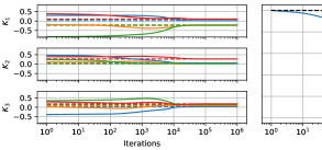
(a)

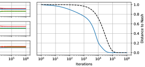
(b)

Figure 1: Convergence of policy gradient in LQ dynamic games to the Nash policy. (a) Each player’s linear feedback gain matrix $K_{i}$ converges to the unique Nash policies (dotted lines). (b) The black dashed line shows upper bound of the number of iterations required to converge within $\varepsilon$ distance from Nash (2-norm). The actual convergence for this random initialization is shown as the solid line.

Consider a four state discrete time linear dynamical system,

$$z(t+1)=Az(t)+B_{1}u_{1}(t)+B_{2}u_{2}(t)+B_{3}u_{3}(t)$$

where $z(t)\in\mathbb{R}^{4}$ and, for each $i\in\{1,2,3\}$, $u_{i}(t)\in\mathbb{R}$ is the control for player $i$. The policy for each player is parameterized by a linear feedback gain matrix, $u_{i}(t)=-K_{i}z(t)$. Moreover, each player seeks to minimize a quadratic cost

$$f_{i}(K_{i},K_{-i})=\mathbb{E}_{z_{0}\sim\mathcal{D}}\left[\sum_{t=0}^{\infty}\left(z(t)^{T}Q_{i}z(t)+\textstyle\sum_{j=1}^{n}u_{j}(t)^{T}R_{ij}u_{j}(t)\right)\right]$$

which is a function of the coupled state variable $z(t)$, their own control $u_{i}(t)$ and all other agents’ control $u_{-i}(t)$ over an infinite time horizon. In an effort to learn a Nash equilibrium, each agent employs policy gradient. In particular, they update their feedback policy via

$$K_{i}(t+1)=K_{i}(t)-\gamma_{i}\nabla_{K_{i}}f_{i}(K_{i},K_{-i}).$$

It is fairly straightforward to compute the gradient of $f_{i}$ with respect to $K_{i}$, the feedback gain that parameterizes player $i$’s control input $u_{i}$. Indeed,

$$\nabla_{K_{i}}f_{i}(K_{i},K_{-i})=2(R_{ii}K_{i}-B_{i}^{T}P_{i}\widetilde{A})\Sigma_{K}$$

where

$$\Sigma_{K}=\mathbb{E}_{z_{0}\sim\mathcal{D}}\left[\sum_{t=0}^{\infty}z(t)z(t)^{T}\right].$$

Hence, the collection of the agents’ individual gradients is given by

$$\omega(K_{1},K_{2},K_{3})=\left(2(R_{ii}K_{i}-B_{i}^{T}P_{i}\widetilde{A})\Sigma_{K}\right)_{i=1}^{3}$$

Remark 4.

Note that $\omega$ can be zero at critical points or at points where $\sum_{t=0}^{\infty}z(t)z(t)^{T}$ drops rank. To prevent the latter possibility, we sample the initial condition from a distribution. That is, we take $z_{0}\sim\mathcal{D}$ so that $\mathbb{E}_{z_{0}\sim\mathcal{D}}z_{0}z_{0}^{T}$ is full rank.

For a given joint policy $(K_{1},K_{2},K_{3})$, the closed loop dynamics are $\widetilde{A}=A-B_{1}K_{1}-B_{2}K_{2}-B_{3}K_{3}$. The states $z(t)$ are obtained from simulating the system. For each $i$, the Riccati matrix $P_{i}$ is computed by solving the Riccati equation

$$P_{i}=\widetilde{A}^{T}P_{i}\widetilde{A}+Q_{i}+\sum_{j=1}^{n}K_{j}R_{ij}K_{j}.$$

Note that this Riccati equation is only used to compute the gradient of the cost functions with respect to a specific set of feedback gains. The system parameters used in this example are listed in Appendix B.1.

For the purpose of validating convergence, we can compute the Nash policies $(K_{1}^{\ast},K_{2}^{\ast},K_{3}^{\ast})$ by an established method with coupled Riccati equations, explained in Appendix B.1. We use the learning rate $\gamma_{i}=\gamma$ defined as in Theorem 1. To compute $\gamma$ we first compute the game Jacobian $J(K_{1}^{*},\ K_{2}^{*},\ K_{3}^{*})$ at the Nash feedback gains and then find the maximum eigenvalue of $J^{T}J$ and minimum eigenvalue of $(J^{T}+J)^{T}(J^{T}+J)$ in a neighborhood of $(K_{1}^{\ast},K_{2}^{\ast},K_{3}^{\ast})$ to determine the constants $\alpha$ and $\beta$ as defined in Section 3.

Figure 1 shows the convergence of the gradient updates to the Nash policies. The $K_{i}$ are randomly initialized in a neighborhood of the known Nash equilibrium and such that $\tilde{A}$ is stable. The number of iterations required to converge to an $\varepsilon$–differential Nash is bounded by the dashed black line in Figure 1b, which shows the curve of $(\varepsilon,T)$ pairs determined by Theorem 1. However, this learning rate is not optimal, as choosing a larger $\gamma$ will result in faster convergence as empirically observed.

Remark 5 (Stochastic Policy Gradient).

We note that stochastic policy gradient with an unbiased estimator has similar convergence properties. Here, e.g., the state dynamics may be subject to zero-mean, finite-variance noise. As long as the estimator for the gradient is unbiased, the theoretical guarantees of the proceeding sections apply.

5.2 Benchmark: matching pennies

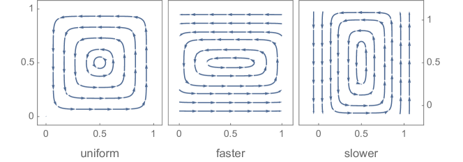
Figure 2: Gradient dynamics of the matching pennies game where agents learning have different learning rates. The vector field of the gradient dynamics are stretched along the faster agent’s coordinate.

The next example is again a multi-agent policy gradient example in which there are two players playing ‘matching pennies’, a classic bimatrix game in which agents have zero-sum costs associated with the matrices $(A,B)$ defined as follows:

$$A=\begin{bmatrix}\ \ \ 1&-1\\ -1&\ \ \ 1\end{bmatrix},\quad B=\begin{bmatrix}-1&\ \ \ 1\\ \ \ \ 1&-1\end{bmatrix}.$$

In particular, the players aim to minimize their respective costs $f_{1}(x,y)=\pi(y)^{T}A\pi(x)$ and $f_{2}(x,y)=\pi(x)^{T}B\pi(y)$ where $\pi(x)$ is player 1’s policy and $\pi(y)$ is player 2’s policy. The class of policies the agents are optimizing over are the so-called ‘softmax’ policies defined by

$$\pi(z)=\left[\frac{e^{10z}}{e^{10z}+e^{10(1-z)}},\quad\frac{e^{10(1-z)}}{e^{10z}+e^{10(1-z)}}\right],$$

and the update each player employs is a ‘smoothed best-response’ which in essence is a policy gradient update with respect to the softmax parameter and each agents individual cost. This game has been well studied in the game theory literature and we use it illustrate the fact that non-uniform learning rates result in a warping of the vector field associated with the agents’ learning dynamics.

The mixed Nash equilibrium for this game is $(x^{\ast},\ y^{\ast})=(0.5,0.5)$, but the Jacobian of the gradient dynamics at this fixed point is

$$J(x^{\ast},\ y^{\ast})=\begin{bmatrix}0&100\\ -100&0\end{bmatrix}$$

so that it has purely imaginary eigenvalues $\pm 100i$, and therefore admits a limit cycle. Regardless, we can visualize the effects of non-uniform learning rates to the gradient dynamics in Figure 2. We notice that the gradient flow stretches along the axes of the faster agent (the agent with a larger learning rate), and the fixed points of these dynamics remain constant.

5.3 Exploring the Effects of Non-uniform Learning Rates on the Learning Path

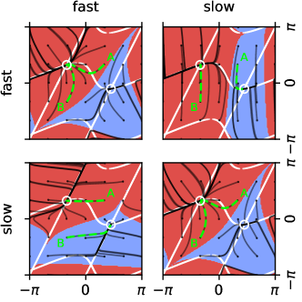
(a)

      

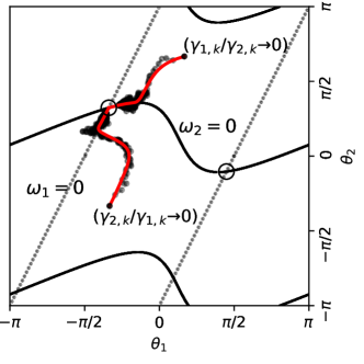
(b)

Figure 3: The effects of non-uniform learning rates on the path of convergence to the equilibria. The zero lines for each player ($D_{1}f_{1}=0$ or $D_{2}f_{2}=0$) are plotted as the diagonal and curved lines, and the two stable Nash equilibria as circles (where $D^{2}_{1}f_{1}>0$ and $D^{2}_{2}f_{2}>0$). (a) In the deterministic setting, the region of attractions for each equilibrium can be computed numerically. Four scenarios are shown, with a combination of fast and slow agents. The region of attractions for each Nash equilibrium are warped under different learning rates. (b) In the stochastic setting, the samples (in black) approximate the singularly perturbed differential equation (in red). Two initializations and learning rate configurations are plotted.

The examples presented so far all consider convergence (or non-convergence) to a single equilibrium. In the following two examples, we investigate the effect of non-uniform learning rates for more general non-convex settings in which there are multiple equilibria. The following example is a two-player game in which the agents’ joint strategy space is a torus. That is, each player’s strategy space is the unit circle $\mathbb{S}^{1}$. For each $i\in\{1,2\}$, player $i$ has cost $f_{i}:\mathbb{S}^{1}\times\mathbb{S}^{1}\to\mathbb{R}$ given by

$$f_{i}(\theta_{i},\theta_{-i})=-\alpha_{i}\cos(\theta_{i}-\phi_{i})+\cos(\theta_{i}-\theta_{-i})$$

where $\alpha_{i}$ and $\phi_{i}$ are constants, and $\theta_{i}$ is player $i$’s choice variable. An interpretation of this game is that of a ‘location game’ in which each player wishes to be near location $\phi_{i}$ but far from each other. This game has many applications including those which abstract nicely to coupled oscillators.

The game form—i.e., collection of individual gradients—is given by

$$\omega(\theta_{1},\theta_{2})=\begin{bmatrix}\alpha_{1}\sin(\theta_{1}-\phi_{1})-\sin(\theta_{1}-\theta_{2})\\ \alpha_{2}\sin(\theta_{2}-\phi_{2})-\sin(\theta_{2}-\theta_{1})\end{bmatrix},$$ (8)

and the game Jacobian is composed of terms $\alpha_{i}\cos(\theta_{i}-\phi_{i})-\cos(\theta_{i}-\theta_{-i})$, $i=1,2$ on the diagonal and $\cos(\theta_{i}-\theta_{-i})$, $i=1,2$ on the off-diagonal.

The Nash equilibria of this game occur where $\omega(\theta_{1},\theta_{2})=0$ and where the diagonals of the game Jacobian are positive. The game has multiple Nash equilibria. We visualize the warping of the region of attraction of these equilibria under different learning rates, and the affinity of the “faster” player to its own zero line.

In this example, we use constants $\phi=(0,\ \pi/8)$ and $\alpha=(1.0,\ 1.5)$. The joint strategy space can be viewed as a non-convex smooth manifold via an equivalence relationship, or equivalently, as players choosing $\theta_{i}\in\mathbb{R}$. There are two Nash equilibria, situated at $(-1.063,\ 1.014)$ and $(1.408,\ -0.325)$. These equilibria happen to also be stable differential Nash, and thus we expect the gradient dynamics to converge to them if initialized in the region of attraction. Which equilibrium it converges to, however, depends on the initialization and learning rates of agents.

To investigate how non-uniform learning rates affect the agents’ convergence to the two equilibria, we simulate agents learning at different rates, one fast and one slow. The fast agent’s learning rate is set to $\gamma_{1}=0.171$ and the slow $\gamma_{2}=0.017$. Figure 3a shows the trajectory of agents’ learned strategies. Each of the four squares depicts the full strategy space on the torus from $-\pi$ to $\pi$ for both agents’ actions, with $\theta_{1}$ on the $x$-axis and $\theta_{2}$ on the $y$-axis. The labels “fast” and “slow” indicate the learning rate of the corresponding agent. For example, in the bottom left square, agent 1 is the fast agent and agent 2 is the slow agent. Hence, the non-uniform update equation for that square becomes $\theta_{k+1}=\theta_{k}-\mathrm{diag}(\gamma_{1},\gamma_{2})\omega(\theta_{k}).$

The white lines indicate the points $x$ such that $\omega_{i}(x)=0$, and the intersection of the white lines indicate points $x$ such that $\omega(x)=0$. The two intersections marked as circles are the stable differential Nash equilibria. The unmarked intersections are either saddle points or other unstable equilibria. The black lines show different paths of the update equations under the non-uniform update equation, with initial points selected from a equally spaced $7\times 7$ grid. We highlight two paths in green (labeled A and B) which begin at $(\pi/3,\ \pi/3)$ and $(-\pi/3,-\pi/3)$.

In the case where agents both learn at the same rate, $(\gamma_{1},\gamma_{1})$ and $(\gamma_{2},\gamma_{2})$, paths A and B both converge to the Nash equilibrium at $(-1.063,\ 1.014)$. However, when agents learn at different rates, the equilibrium to which the agents converge to, as well as the learning path, is no longer the same even starting at the same initial points. This phenomena can also be captured by displaying the region of attraction for both Nash equilibria. The red region corresponds to initializations that will converge to the equilibrium contained in the red region (again indicated by a white circle). Analogously, the blue region corresponds to the region of attraction of the other equilibria.

To provide an example of the stochastic setting in which agents have an unbiased estimator of their individual gradients, we choose learning rates according to Assumption 2. In particular, we choose scaled learning rates $\gamma_{2,k}=\frac{1}{1+k\log(k+1)}$ and $\gamma_{1,k}=\frac{1}{1+k}$ such that $\gamma_{2,k}/\gamma_{1,k}\to 0$ as $k\to\infty$. Figure 3b shows the learning paths in this setting initialized at two different points, each with flipped learning rate configurations. The sample points approximate the singularly perturbed differential equation (shown in red) described in Section 4.2.

In both deterministic and stochastic settings, we observe the affinity of the faster agent to its own zero line. For example, the bottom left square (in Figure 3a) and bottom left path (in Figure 3b) both have agent 1 as the faster agent, and the learning paths both tend to arrive to the line $\omega_{1}\equiv 0$ before finally converging to the Nash equilibrium. An interpretation of this is that the faster agent tries to be situated at the bottom of the “valley” of its own cost function. The faster agent tends to be at its own minimum while it waits for the slower agent to change its strategy. As a Stackelberg interpretation, where there are followers and leaders, the slower agent would be the leader and faster agent the follower. In a sense, the slower agent has an advantage.

5.4 Multi-agent control and collision avoidance

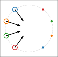
(a)

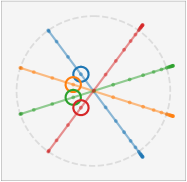
(b)

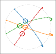
(c)

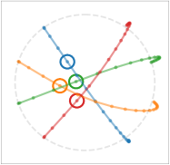
(d)

Figure 4: Minimum-fuel particle avoidance control example. (a) Each particle seeks to reach the opposite side of the circle using minimum fuel while avoiding each other. The circles represent the approximate boundaries around each particle at time $t=5$. (b) The joint strategy $x=({\bf u}_{1},\cdots,{\bf u}_{4})$ is initialized to the minimum fuel solution ignoring interaction between particles. (c) Equilibrium solution achieved by setting the blue agent to have a slower learning rate. (d) Another equilibrium, where the red agent has the slower learning rate.

The final example presents a practical use case for the gradient-based update. Consider a non-cooperative game between four collision-avoiding agents where they seek to arrive at a destination with minimum fuel while avoiding each other. We show that the scaling between agents’ learning rates dictates the equilibrium solution to which they converges. This can be useful in designing non-cooperative open-loop controllers where agents may choose to learn slower in order to deviate less from their initial plan, perhaps in an attempt to incur less ‘risk’.

Suppose there are four collision-avoiding particles traversing across a unit circle. Each particle follows discrete-time linear dynamics

$$z_{i}(t+1)=Az_{i}(t)+Bu_{i}(t)$$

for $t=1,\cdots,N$ where

$$A=\begin{bmatrix}I&hI\\ 0&I\end{bmatrix}\in\mathbb{R}^{4\times 4},\ B=\begin{bmatrix}h^{2}I\\ hI\end{bmatrix}\in\mathbb{R}^{4\times 2},$$

$I$ is the identity matrix, and $h=0.1$. These dynamics represent a typical discretized version of the continuous dynamics $\ddot{r}_{i}=u_{i}$ in which $u_{i}\in\mathbb{R}^{2}$ represents a force vector used to accelerate the particle, and the state $z_{i}=[r_{i},\dot{r}_{i}]$ represents the particles position and velocity. Let ${\bf u}_{i}$ be the concatenated vector of control vectors for player $i$ for all time—i.e., ${\bf u}_{i}=(u_{i}(1),\cdots,u_{i}(N))$ and let ${\bf u}=({\bf u}_{1},\cdots,{\bf u}_{n})$. Each particle $i$ aims to minimize a cost defined by

$$J_{i}({\bf u}) =\sum_{t=1}^{N}\|u_{i}(t)\|_{R}^{2}+\sum_{t=1}^{N+1}\|z_{i}(t)-\bar{z_{i}}\|_{Q}^{2}+\sum_{j\neq i}\sum_{t=1}^{N+1}\rho e^{-\sigma\|z_{i}(t)-z_{j}(t)\|_{S}^{2}}$$

where $\|\cdot\|_{P}$ denotes the quadratic norm—i.e., $\|z\|_{P}^{2}=z^{T}Pz$ with $P$ positive semi-definite. The first two terms of the cost correspond to the minimum fuel objective and quadratic cost from desired final state $\bar{z}_{i}$, a typical setup for optimal control problems. We use $R=\mathrm{diag}(0.1,0.1)$ and $Q=\mathrm{diag}(1,1,0,0)$. The final term of the cost function is the sum of all pairwise interaction terms between the particles, modeled after the shape of a Gaussian which encodes smooth boundaries around the particles. We use constants $\rho=10$ and $\sigma=100$.

Figure 4 (a) visualizes the problem setup. Each particle’s initial position $z_{i}(0)$ is located on the left side of a unit circle; they are separated by $\pi/5$, and their desired final positions, $\bar{z_{i}}$ for each $i\in\{1,\ldots,4\}$, are located directly opposite. The particles begin with zero velocity and must solve for a minimum control solution that also avoids collision with other particles as described by the objectives $J_{i}$ for each $i$.

To initialize the gradient-based learning algorithms in the game setting, we compute the optimal solution for each agent ignoring the pairwise interaction terms, shown in Figure 4 (b). This can be computed using classical discrete-time LQR methods or by gradient descent. Then, using this solution as the intialization for the game setting, each agent descends their own gradient, i.e.

$${\bf u}_{i,k+1}={\bf u}_{i,k}-\gamma_{i}D_{i}J_{i}({\bf u}),$$

with different learning rates $\gamma_{i}$. Just as the previous example shows, the relative learning rates of agents warp the region of attraction for the multiple equilibria. If we allow the red agent to learn slower, then the learning process converges to the equilibria shown in Figure 4 (c), whereas if the blue agent learns quicker, then we converge to Figure 4 (d). Hence, all else being equal, the learning rates adopted by players greatly impact the equilibrium to which they converge.

6 Discussion and Future Work

We analyze the convergence of gradient-based learning for non-cooperative agents with continuous costs. We leverage existing dynamical systems theory and stochastic approximation literature to provide convergence guarantees for agents that learn myopically—that is, only using information about their own gradient $D_{i}f_{i}$ to update their strategy. We provide guarantees for the case where agents are assumed to have oracle access to $D_{i}f_{i}$ and the case where they have sufficient information to compute an unbiased estimator. We also study the effects of non-uniform learning rates.

By preconditioning the gradient dynamics by $\Gamma$, a diagonal matrix where the diagonals represent the agents’ learning rates, we can begin to understand how a changing learning rate relative to others can change the properties of the fixed points of the dynamics. Moreover, players do not know how a change in others’ strategies affects its own cost ($D_{j}f_{i}$ where $j\neq i$). A possible extension to this paper is to develop update schemes that use this to provide more robust convergence guarantees for full information continuous games. Different learning rates amongst agents also affects the region of attraction of the game, hence starting from the same initial condition, agents may converge to a different equilibria. Agents may use this to their benefit, as shown in the last example. Such insights into the learning behavior of agents will be useful for providing guarantees on the design of control or incentive policies to coordinate agents. We also show through numerical examples that, counterintuitively, if an agent decides to learn slower, a stable differential Nash equilibrium can go unstable, resulting in learning dynamics that do not converge to Nash.

Beyond the the effects of learning rates, there are a number of avenues for future inquiry. For instance, the results as stated apply to continuous games with Euclidean strategy spaces. An interesting avenue to pursue is the study of learning in games where the agents decision spaces are constrained sets or Riemannian manifolds. The latter arises in a number of robotics applications and in this case, the update rule will need to be modified by the appropriately defined retraction such as $x_{k+1}=\exp_{x_{k}}(\gamma_{k}(\omega(x_{k})))$ [31]. The former arises in a variety of applications where the learning rules are abstractions of agents learning in, e.g., physically constrained environments. The update rule in this case will also need to be defined in terms of the appropriate proximal map thereby leading to potentially non-smooth dynamics [10, 19] which is even more challenging in the stochastic setting. Yet, such extensions will lead to a framework and set of analysis tools that apply to a broader class of multi-agent learning algorithms.

While we present the work in the context of gradient-based learning in games, there is nothing that precludes the results from applying to update rules in other frameworks. Our results will apply to many other settings where agents myopically update their decision using a process of the form $x_{k+1}=x_{k}-\Gamma g(x_{k})$. In this paper, we consider the special case where $g\equiv[D_{1}f_{1}\cdots D_{n}f_{n}]$. In the stochastic setting, variants of multi-agent Q-learning conform to this setting since Q-learning can be written as a stochastic approximation update.

Finally, as pointed out in [21], not all critical points of the dyanamics $\dot{x}=-\omega(x)$ that are attracting are necessarily Nash equilibria; one can see this simply by constructing a Jacobian with positive eigenvalues with at least one $D^{2}_{i}f_{i}$ with a non-positive eigenvalue. Understanding this phenomena will help us develop computational techniques to avoid them. Recent work has explored this in the context of zero-sum games [22], requiring coordination amongst the learning agents. However, when our objective is to study the learning behavior of autonomous agents seeking an equilibrium, an alternative perspective is needed.

A Proofs

A.1 Deterministic Setting

The following proof follows nearly the same proof as the main result in [2] with a few minor modifications in the conclusion; we provide it here for posterity.

• Since $\|I-\Gamma D\omega(x)\|<1$ for each $x\in B_{r_{0}}(x^{\ast})$, as stated in the proposition statement, there exists $0<r^{\prime}<r^{\prime\prime}<1$ such that $\|I-\Gamma D\omega(x)\|\leq r^{\prime}<r^{\prime\prime}<1$ for all $x\in B_{r}(x^{\ast})$. Since

  $$\lim_{x\rightarrow x^{\ast}}\|R(x-x^{\ast})\|/\|x-x^{\ast}\|=0,$$

  for $0<1-r^{\prime\prime}<1$, there exists $\tilde{r}>0$ such that

  $$\|R(x-x^{\ast})\|\leq(1-r^{\prime\prime})\|x-x^{\ast}\|,\ \ \forall\ x\in B_{\tilde{r}}(x^{\ast}).$$

  As in the proposition statement, let $r$ be the largest, finite such $\tilde{r}$. Note that for arbitrary $c>0$, there exists $\tilde{r}>0$ such that the bound on $\|R(x-x^{\ast})\|$ holds; hence, we choose $c=1-r^{\prime\prime}$ and find the largest such $\tilde{r}$ for which the bound holds. Combining the above bounds with the definition of $g$, we have that

  $$\|g(x)-g(x^{\ast})\|\leq(1-\delta)\|x-x^{\ast}\|,\ \ \forall\ x\in B_{r^{\ast}}(x^{\ast})$$

  where $\delta=r^{\prime\prime}-r^{\prime}$ and $r^{\ast}=\min\{r_{0},r\}$. Hence, applying the result iteratively, we have that

  $$\|x_{t}-x^{\ast}\|\leq(1-\delta)^{t}\|x_{0}-x^{\ast}\|,\ \ \forall\ x_{0}\in B_{r^{\ast}}(x^{\ast}).$$

  Note that $0<1-\delta<1$. Using the approximation $1-\delta<\exp(-\delta)$, we have that

  $$\|x_{T}-x^{\ast}\|\leq\exp(-T\delta)\|x_{0}-x^{\ast}\|$$

  so that $x_{t}\in B_{\varepsilon}(x^{\ast})$ for all $t\geq T=\lceil\delta^{-1}\log(r^{\ast}/\varepsilon)\rceil$.

∎

As noted in the remark, a similar result holds under the relaxed assumption that $\rho(I-\Gamma D\omega(x))<1$ for all $x\in B_{r_{0}}(x^{\ast})$. To see this, we first note that $\rho(I-\Gamma D\omega(x))<1$ implies there exists $c>0$ such that $\rho(I-\Gamma D\omega(x))\leq c<1$. Hence, given any $\epsilon>0$, there is a norm on $\mathbb{R}^{d}$ and a $c>0$ such that $\|I-\Gamma D\omega\|\leq c+\epsilon<1$ on $B_{r_{0}}(x^{\ast})$ [25, 2.2.8]. Then, we can apply the same argument as above using $r^{\prime}=c+\varepsilon$.

A.2 Stochastic Setting

A key tool used in the finite-time two-timescale analysis is the nonlinear variation of constants formula of Alekseev [1], [9].

Theorem 6.

Consider a differential equation

$$\dot{u}(t)=f(t,u(t)),\ t\geq 0,$$

and its perturbation

$$\dot{p}(t)=f(t,p(t))+\tilde{f}(t,p(t)),\ t\geq 0$$

where $f,\tilde{f}:\mathbb{R}\times\mathbb{R}^{d}\rightarrow\mathbb{R}^{d}$, $f\in C^{1}$, and $\tilde{f}\in C$. Let $u(t,t_{0},p_{0})$ and $p(t,t_{0},p_{0})$ denote the solutions of the above nonlinear systems for $t\geq t_{0}$ satisfying $u(t_{0},t_{0},p_{0})=p(t_{0},t_{0},p_{0})=p_{0}$, respectively. Then,

$$p(t,t_{0},p_{0}) =u(t,t_{0},p_{0})+\int_{t_{0}}^{t}\Phi(t,s,p(s,t_{0},p_{0}))\tilde{f}(s,p(s,t_{0},p_{0}))\ ds,\ t\geq t_{0}$$

where $\Phi(t,s,u_{0})$, for $u_{0}\in\mathbb{R}^{d}$, is the fundamental matrix of the linear system

$$\dot{v}(t)=\frac{\partial f}{\partial u}(t,u(t,s,u_{0}))v(t),\ t\geq s$$ (9)

with $\Phi(s,s,u_{0})=I_{d}$, the $d$–dimensional identity matrix.

Consider a locally asymptotically stable differential Nash equilibrium $x^{\ast}=(\lambda(x_{2}^{\ast}),x_{2}^{\ast})\in X$ and let $B_{r_{0}}(x^{\ast})$ be an ${r}_{0}>0$ radius ball around $x^{\ast}$ contained in the region of attraction. Stability implies that the Jacobian $J(\lambda(x_{2}^{\ast}),x_{2}^{\ast})$ is positive definite and by the converse Lyapunov theorem [30, Chapter 5] there exists local Lyapunov functions for the dynamics $\dot{x}_{2}(t)=-\tau D_{2}f_{2}(\lambda(x_{2}(t)),x_{2}(t))$ and for the dynamics $\dot{x}_{1}(t)=-D_{1}f_{1}(x_{1}(t),x_{2})$, for each fixed $x_{2}$. In particular, there exists a local Lyapunov function $V\in C^{1}(\mathbb{R}^{d_{1}})$ with $\lim_{\|x_{2}\|\uparrow\infty}V(x_{2})=\infty$, and $\langle\nabla V(x_{2}),D_{2}f_{2}(\lambda(x_{2}),x_{2})\rangle<0$ for $x_{2}\neq x_{2}^{\ast}$. For $r>0$, let $V^{r}=\{x\in\text{dom}(V):\ V(x)\leq r\}$. Then, there is also $r>r_{0}>0$ and $\epsilon_{0}>0$ such that for $\epsilon<\epsilon_{0}$,

$$\{x_{2}\in\mathbb{R}^{d_{2}}|\ \|x_{2}-x_{2}^{\ast}\|\leq\epsilon\}\subseteq V^{r_{0}}\subset\mathcal{N}_{\epsilon_{0}}(V^{r_{0}})\subseteq V^{r}\subset\text{dom}(V)$$

where $\mathcal{N}_{\epsilon_{0}}(V^{r_{0}})=\{x\in\mathbb{R}^{d_{2}}|\ \exists x^{\prime}\in V^{r_{0}}\ \text{s.t.}\|x^{\prime}-x\|\leq\epsilon_{0}\}$. An analogously defined $\tilde{V}$ exists for the dynamics $\dot{x}_{1}$ for each fixed $x_{2}$.

For now, fix $n_{0}$ sufficiently large; we specify this a bit further down. Define the event

$$\mathcal{E}_{k}=\{\bar{x}_{1}(t)\in V^{r}\ \forall t\in[\tilde{t}_{k_{0}},\tilde{t}_{k}]\}$$

where

$$\bar{x}_{1}(t)=x_{1,k}+\frac{t-\tilde{t}_{k}}{\gamma_{1,k}}(x_{1,k+1}-x_{1,k})$$

are linear interpolates defined for $t\in(\tilde{t}_{k},\tilde{t}_{k+1})$ with $\tilde{t}_{k+1}=\tilde{t}_{k}+\gamma_{1,k}$ and $\tilde{t}_{0}=0$. The basic idea of the proof is to leverage Alekseev’s formula (Theorem 6) to bound the difference between the linearly interpolated trajectories (i.e., asymptotic psuedo-trajectories) and the flow of the corresponding limiting differential equation on each continuous time interval between each of the successive iterates $k$ and $k+1$ by a number that decays asymptotically. Then, for large enough $k$, a union bound is used over all the remaining time intervals to construct a concentration bound. This is done first for fast player (i.e. player 1), to show that $x_{1,k}$ tracks $\lambda(x_{2,k})$, and then for the slow player (i.e., player 2).

Following Borkar and Pattathil [9], we can express the linear interpolates for any $k\geq k_{0}$ as $\bar{x}_{1}(\tilde{t}_{k+1})\textstyle=\bar{x}_{1}(\tilde{t}_{k_{0}})-\sum_{\ell=k_{0}}^{n}\gamma_{1,\ell}(D_{1}f_{1}(x_{\ell})+w_{1,\ell+1})$ where

$$\gamma_{1,\ell}D_{1}f_{1}(x_{\ell})=\int_{\tilde{t}_{\ell}}^{\tilde{t}_{\ell+1}}D_{1}f_{1}(\bar{x}_{1}(\tilde{t}_{\ell}),x_{2,\ell})$$

and similarly for the $w_{1,\ell+1}$ term. Adding and subtracting $\int_{\tilde{t}_{n_{0}}}^{\tilde{t}_{n+1}}D_{1}f_{1}(\bar{x}_{1}(s),x_{2}(s))$, Alekseev’s formula can be applied to get

$$\bar{x}_{1}(t) =x_{1}(t)+\Phi_{1}(t,s,\bar{x}_{1}(\tilde{t}_{k_{0}}),x_{2}(\tilde{t}_{k_{0}}))(\bar{x}_{1}(\tilde{t}_{k_{0}})-x_{1}(\tilde{t}_{k_{0}}))+\int_{\tilde{t}_{k_{0}}}^{t}\Phi_{2}(t,s,\bar{x}_{1}(s),x_{2}(s))\zeta_{1}(s)\ ds$$

where $x_{2}(t)\equiv x_{2}$ is constant (since $\dot{x}_{2}=0$), $x_{1}(t)=\lambda(x_{2})$,

$$\zeta_{1}(s)=-D_{1}f_{1}(\bar{x}_{1}(\tilde{t}_{k}),x_{2}(\tilde{t}_{k}))+D_{1}f_{1}(\bar{x}_{1}(s),x_{2}(s))+w_{1,k+1},$$

and where for $t\geq s$, $\Phi_{1}(\cdot)$ satisfies linear system

$$\dot{\Phi}_{1}(t,s,x_{0})=J_{1}(x_{1}(t),x_{2}(t))\Phi_{1}(t,s,x_{0}),$$

with initial data $\Phi_{1}(t,s,x_{0})=I$ and $x_{0}=(x_{1,0},x_{2,0})$ and where $J_{1}$ the Jacobian of $-D_{1}f_{1}(\cdot,x_{2})$.

Given that $x^{\ast}=(\lambda(x_{2}^{\ast}),x_{2}^{\ast})$ is a stable differential Nash equilibrium, $J_{1}(x^{\ast})$ is positive definite. Hence, as in [32, Lemma 5.3], we can find $M$, $\kappa_{1}>0$ such that for $t\geq s$, $x_{1,0}\in V^{r}$, $\|\Phi_{1}(t,s,x_{1,0},x_{2,0})\|\leq Me^{-\kappa_{1}(t-s)}$; this result follows from standard results on stability of linear systems (see, e.g., Callier and Desoer [11, §7.2, Theorem 33]) along with a bound on

$$\int_{s}^{t}\|D^{2}_{1}f_{1}(x_{1},x_{2}(\tau,s,\tilde{x}_{0}))-D_{1}^{2}f_{1}(x^{\ast})\|d\tau$$

for $\tilde{x}_{0}\in V^{r}$ (see, e.g., [32, Lemma 5.2]).

Consider $z_{k}=\lambda(x_{2,k})$—i.e., where $D_{1}f_{1}(x_{1,k},x_{2,k})=0$. Then, using a Taylor expansion of the implicitly defined $\lambda$, we get

$$z_{k+1}=z_{k}+D\lambda(x_{2,k})(x_{2,k+1}-x_{2,k})+\delta_{k+1}$$ (10)

where $\|\delta_{k+1}\|\leq L_{r}\|x_{2,k+1}-x_{2,k}\|^{2}$ is the error from the remainder terms. Plugging in $x_{2,k+1}$, we have

$$z_{k+1} =z_{k}+\gamma_{1,k}(-D_{1}f_{1}(z_{k},x_{2,k})+\tau_{k}\lambda(x_{2,k})(w_{2,k+1}-D_{2}f_{2}(x_{1,k},x_{2,k}))+\gamma_{1,k}^{-1}\delta_{k+1}).$$

The terms after $-D_{1}f_{1}$ are $o(1)$, and hence asymptotically negligible, so that this $z$ sequence tracks dynamics as $x_{1,k}$. We show that with high probability, they asymptotically contract to one another.

Define constant $H_{k_{0}}=(\|\bar{x}_{1}(\tilde{t}_{k_{0}}-x_{1}(\tilde{t}_{k_{0}})\|+\|\bar{z}(\tilde{t}_{k_{0}})-x_{1}(\tilde{t}_{k_{0}})\|)$ and

$$S_{1,k} =\sum_{\ell=k_{0}}^{k-1}\Big{(}\int_{\tilde{t}_{\ell}}^{\tilde{t}_{\ell+1}}\Phi_{1}(\tilde{t}_{k},s,\bar{x}_{1}(\tilde{t}_{\ell}),x_{2}(\tilde{t}_{\ell}))ds\Big{)}w_{2,\ell+1}.$$

Moreover, let $\tau_{k}=\gamma_{2,k}/\gamma_{1,k}$.

Lemma 2.

For any $k\geq k_{0}$, there exists $K>0$ such that

$$\|x_{1,k}-z_{k}\|\leq K\Big{(}\|S_{1,k}\|+e^{-\kappa_{1}(\tilde{t}_{k}-\tilde{t}_{k_{0}})}H_{k_{0}}+\sup_{k_{0}\leq\ell\leq k-1}\gamma_{1,\ell}+\sup_{k_{0}\leq\ell\leq k-1}\gamma_{1,\ell}\|w_{1,\ell+1}\|^{2}$$

$$+\sup_{k_{0}\leq\ell\leq k-1}\tau_{\ell}+\sup_{k_{0}\leq\ell\leq k-1}\tau_{\ell}\|w_{2,\ell+1}\|^{2}\Big{)}$$

conditioned on ${\mathcal{E}}_{k}$.

In order to construct a high-probability bound for $x_{2,k}$, we need a similar bound as in Lemma 2 can be constructed for $x_{2,k}$. Define the event $\hat{\mathcal{E}}_{k}=\{\bar{x}_{2}(t)\in V^{{r}}\ \forall t\in[\hat{t}_{k_{0}},\hat{t}_{k}]\}$ where $\bar{x}_{2}(t)=x_{2,k}+\frac{t-\hat{t}_{k}}{\gamma_{2,k}}(x_{2,k+1}-x_{2,k})$ is the linear interpolated points between the samples $\{x_{2,k}\}$, $\hat{t}_{k+1}=\hat{t}_{k}+\gamma_{1,k}$, and $\hat{t}_{0}=0$. Then as above, Alekseev’s formula can again be applied to get

$$\bar{x}_{2} (t)=x_{2}(t,\hat{t}_{k_{0}},x_{2}(\hat{t}_{k_{0}}))+\Phi_{2}(t,\hat{t}_{k_{0}},\bar{x}_{2}(\hat{t}_{k_{0}}))(\bar{x}_{2}(\hat{t}_{k_{0}})-x_{2}(\hat{t}_{k_{0}}))+\int_{\hat{t}_{k_{0}}}^{t}\Phi_{2}(t,s,\bar{x}_{2}(s))\zeta_{1}(s)\ ds$$

where $x_{2}(t)\equiv x_{2}^{\ast}$,

$$\zeta_{1}(s) =D_{2}f_{2}(\lambda(x_{2,k}),x_{2,k})-D_{2}f_{2}(\lambda(\bar{x}_{2}(s)),\bar{x}_{2}(s))+D_{2}f_{2}(x_{k})-D_{2}f_{2}(\lambda(x_{2,k}),x_{2,k})+w_{2,k+1},$$

and $\Phi_{2}$ is the solution to a linear system with dynamics $J_{2}(\lambda(x_{2}^{\ast}),x_{2}^{\ast})$, the Jacobian of $-D_{2}f_{2}(\lambda(\cdot),\cdot)$, and with initial data $\Phi_{2}(s,s,x_{2,0})=I$. This linear system, as above, has bound $\|\Phi_{2}(t,s,x_{2,0})\|\leq M_{2}e^{\kappa_{2}(t-1)}$ for some $M_{2},\kappa_{2}>0$. Define

$$S_{2,k} =\sum_{\ell=k_{0}}^{k-1}\Big{(}\int_{\hat{t}_{\ell}}^{\hat{t}_{\ell+1}}\Phi_{2}(\hat{t}_{k},s,\bar{x}_{2}(\hat{t}_{\ell}))ds\Big{)}w_{2,\ell+1}.$$

Lemma 3.

For any $k\geq k_{0}$, there exists $\bar{K}>0$ such that

$$\|\bar{x}_{2}(\hat{t}_{k})-x_{2}(\hat{t}_{k})\|\leq \textstyle\bar{K}\big{(}\|S_{2,k}\|+\sup_{k_{0}\leq\ell\leq k-1}\|S_{1,\ell}\|\textstyle+\sup_{k_{0}\leq\ell\leq k-1}\gamma_{1,\ell}+\sup_{k_{0}\leq\ell\leq k-1}\gamma_{1,\ell}\|w_{1,\ell+1}\|^{2}$$

$$\textstyle+\sup_{k_{0}\leq\ell\leq k-1}\tau_{\ell}+\sup_{k_{0}\leq\ell\leq k-1}\tau_{\ell}\|w_{2,\ell+1}\|^{2}\textstyle+e^{\kappa_{2}(\hat{t}_{k}-\hat{t}_{k_{0}})}\|\bar{x}_{2}(\hat{t}_{k_{0}})-x_{2}(\hat{t}_{k_{0}})\|$$

$$\textstyle+\sup_{k_{0}\leq\ell\leq k-1}\tau_{k}H_{k_{0}}\big{)}$$

conditioned on $\tilde{\mathcal{E}}_{k}$.

Using the above lemmas, we can get the desired guarantees on $x_{1,k}$ and $x_{2,k}$ as in [9].

B Additional Examples

In this appendix, we include additional examples and information about examples contained in the main body of the text.

B.1 LQ game system parameters

The following are the system parameters and resulting Nash feedback gains computed using the coupled Riccatti equations:

$$A=\begin{bmatrix}0.402&1.037&-0.565&0.115\\ -0.021&-0.990&-0.584&0.457\\ 0.377&1.105&0.698&1.192\\ -0.177&-0.332&0.237&-0.286\end{bmatrix},\ B_{1}=\begin{bmatrix}1\\ 1\\ 0\\ 0\end{bmatrix},\ B_{2}=\begin{bmatrix}0\\ 1\\ 1\\ 0\end{bmatrix}\,B_{3}=\begin{bmatrix}0\\ 0\\ 1\\ 1\end{bmatrix}$$

$$Q_{1}=\begin{bmatrix}0.48&0&0&0\\ 0&0.64&0&0\\ 0&0&0.74&0\\ 0&0&0&0.71\end{bmatrix},\ Q_{2}=\begin{bmatrix}0.01&0&0&0\\ 0&0.41&0&0\\ 0&0&0.71&0\\ 0&0&0&0.44\end{bmatrix},\ Q_{3}=\begin{bmatrix}1.00&0&0&0\\ 0&0.55&0&0\\ 0&0&0.86&0\\ 0&0&0&0.63\end{bmatrix},$$

$$R_{11}=\begin{bmatrix}5.47\end{bmatrix},\ R_{12}=\begin{bmatrix}7.16\end{bmatrix},\ R_{13}=\begin{bmatrix}5.31\end{bmatrix},\ R_{21}=\begin{bmatrix}5.21\end{bmatrix},\ R_{22}=\begin{bmatrix}5.36\end{bmatrix},$$

$$R_{23}=\begin{bmatrix}7.63\end{bmatrix},\ R_{31}=\begin{bmatrix}9.71\end{bmatrix},\ R_{32}=\begin{bmatrix}2.34\end{bmatrix},\ R_{33}=\begin{bmatrix}5.26\end{bmatrix},\$$

and

$$K_{1}=\begin{bmatrix}0.023\\ -0.201\\ -0.228\\ 0.104\end{bmatrix}^{T},K_{2}=\begin{bmatrix}0.060\\ 0.029\\ 0.026\\ 0.274\end{bmatrix}^{T},K_{3}=\begin{bmatrix}0.033\\ 0.082\\ 0.138\\ 0.177\end{bmatrix}^{T}.$$

We use the following values for constants used in the LQ game: $\alpha=19.4$ and $2.90\times 10^{5}$; hence, we use $\gamma=1.52\times 10^{-5}$.

B.2 Coupled Riccati equations

We require the following standard assumption adopted in LQ games.

Assumption 5.

Either $(A,B_{1},\sqrt{Q_{1}})$ or $(A,B_{2},\sqrt{Q_{2}})$ is stabilizable-detectable.

Without loss of generality, we assume $(A,B_{1},\sqrt{Q_{1}})$ is stabilizable-detectable. We employ the following iterative Lyapunov algorithm for finding the Nash equilibrium to the linear quadratic game [20]:

step 1.

Initialize $P_{1}^{(0)}$ to be the unique positive definite solution to the Riccati equation,

$$P_{1}^{(0)}=A^{T}P_{1}^{(0)}A-A^{T}P_{1}^{(0)}B_{1}\big{(}R_{1}+B_{1}^{T}P_{1}^{(0)}B_{1}\big{)}^{-1}B_{1}^{T}P_{1}^{(0)}A+Q_{1},$$ (11)

and compute the corresponding gain matrix for player 1 by

$$K_{1}^{(0)} =(R_{1}+B_{1}^{T}P_{1}^{(0)}B_{1})^{-1}B_{1}^{T}P_{1}^{(0)}A.$$ (12)

Solve for $P_{2}^{(0)}$ by

$$P_{2}^{(0)}=\bar{A}^{T}P_{2}^{(0)}\bar{A}-\bar{A}^{T}P_{2}^{(0)}B_{2}\big{(}R_{2}+B_{2}^{T}P_{2}^{(0)}B_{2}\big{)}^{-1}B_{2}^{T}P_{2}^{(0)}\bar{A}+Q_{1}$$ (13)

where $\bar{A}=A-B_{1}K_{1}^{(0)}$ and compute the corresponding gain matrix for player 2 by

$$K_{2}^{(0)} =(R_{2}+B_{2}^{T}P_{2}^{(0)}B_{2})^{-1}B_{2}^{T}P_{2}^{(0)}\big{(}A-B_{1}K_{1}^{(0)}\big{)}.$$ (14)

We note that initializing using this method ensures that the initial closed loop matrix $A-B_{1}K_{1}^{(0)}-B_{2}K_{2}^{(0)}$ is stable.

step 2.

Given $P_{1}^{(k)}$, $P_{2}^{(k)}$, $K_{1}^{(k)}$, and $K_{2}^{(k)}$, update the feedback gains using the following update rules:

$$K_{1}^{(k+1)} =(R_{11}+B_{1}^{T}P_{1}^{(k)}B_{1})^{-1}B_{1}^{T}P_{1}^{(k)}(A-B_{2}K_{2}^{(k)})$$ (15)

$$K_{2}^{(k+1)} =(R_{22}+B_{2}^{T}P_{2}^{(k)}B_{2})^{-1}B_{2}^{T}P_{2}^{(k)}(A-B_{1}K_{1}^{(k)})$$ (16)

step 3.

Update the cost-to-go matrices by solving the Lyapunov equations:

$$P_{1}^{(k)} = (\bar{A}-B_{2}K_{2}^{(k)})^{T}P_{1}^{(k+1)}(\bar{A}-B_{2}K_{2}^{(k)})+(K_{1}^{(k)})^{T}R_{11}K_{1}^{(k)}+(K_{2}^{(k)})^{T}R_{12}K_{2}^{(k)}+Q_{1}$$

$$P_{2}^{(k)} = (\bar{A}-B_{2}K_{2}^{(k)})^{T}P_{2}^{(k+1)}(\bar{A}-B_{2}K_{2}^{(k)})+(K_{1}^{(k)})^{T}R_{21}K_{1}^{(k)}+(K_{2}^{(k)})^{T}R_{22}K_{2}^{(k)}+Q_{2}$$

step 4.

Repeat steps 2–3 until the gains converge.

The extension to $n$-players is fairly straightforward; more detail can be found in the seminal reference [4].

References

• Alekseev [1961] V. M. Alekseev. An estimate for the perturbations of the solutions of ordinary differential equations. Vestnik Moskov. Univ. Ser. I. Mat. Meh., 2:28–36, 1961.
• Argyros [1999] I. K. Argyros. A generalization of ostrowski’s theorem on fixed points. Applied Mathematics Letters, 12:77–79, 1999.
• Balduzzi et al. [2018] David Balduzzi, Sébastien Racaniere, James Martens, Jakob Foerster, Karl Tuyls, and Thore Graepel. The mechanics of n-player differentiable games. CoRR, abs/1802.05642, 2018.
• Basar and Olsder [1998] T. Basar and G. Olsder. Dynamic Noncooperative Game Theory. Society for Industrial and Applied Mathematics, 2nd edition, 1998. doi: 10.1137/1.9781611971132.
• Benaïm [1999] Michel Benaïm. Dynamics of stochastic approximation algorithms. In Seminaire de Probabilites XXXIII, pages 1–68, 1999.
• Benaim and Hirsch [1999] Michel Benaim and Morris W. Hirsch. Mixed equilibria and dynamical systems arising from fictitious play in perturbed games. Games and Economic Behavior, 29(1-2):36–72, 1999.
• Benaïm et al. [2012] Michel Benaïm, Josef Hofbauer, and Sylvain Sorin. Perturbations of set-valued dynamical systems, with applications to game theory. Dynamic Games and Applications, 2(2):195–205, 2012.
• Bhatnagar and Prasad [2013] S. Bhatnagar and H. L. Prasad. Stochastic Recursive Algorithms for Optimization. Springer, 2013.
• Borkar and Pattathil [2018] Vivek S. Borkar and Sarath Pattathil. Concentration bounds for two time scale stochastic approximation. arxiv:1806.10798, 2018.
• Borkar [2008] V.S. Borkar. Stochastic Approximation: A Dynamical Systems Viewpoint. Springer, 2008.
• Callier and Desoer [1991] F. Callier and C. Desoer. Linear Systems Theory. Springer, 1991.
• Daskalakis et al. [2017] Constantinos Daskalakis, Andrew Ilyas, Vasilis Syrgkanis, and Haoyang Zeng. Traning GANs with Optimism. arxiv:1711.00141, 2017.
• Fudenberg and Levine [1998] Drew Fudenberg and David K Levine. The theory of learning in games, volume 2. MIT press, 1998.
• Hart and Mas-Colell [2003] Sergiu Hart and Andreu Mas-Colell. Uncoupled dynamics do not lead to nash equilibrium. American Economic Review, 93(5):1830–1836, December 2003. doi: 10.1257/000282803322655581.
• Heinrich and Silver [2016] J. Heinrich and D. Silver. Deep reinforcement learning from self-play in imperfect-information games. arxiv:1603.01121, 2016.
• Hofbauer [1996] Josef Hofbauer. Evolutionary dynamics for bimatrix games: A hamiltonian system? Journal of Mathematical Biology, 34(5):675, May 1996.
• Hommes and Ochea [2012] Cars H. Hommes and Marius I. Ochea. Multiple equilibria and limit cycles in evolutionary games with logit dynamics. Games and Economic Behavior, 74(1):434 –441, 2012. doi: 10.1016/j.geb.2011.05.014.
• Karmakar and Bhatnagar [2018] Prasenjit Karmakar and Shalabh Bhatnagar. Two time-scale stochastic approximation with controlled markov noise and off-policy temporal-difference learning. Mathematics of Operations Research, 2018.
• Kushner and Yin [2003] H. J. Kushner and G. G. Yin. Stochastic Approximation and Recursive Algorithms and Applications. Springer, 2nd edition, 2003.
• Li and Gajic [1995] T-Y. Li and Z. Gajic. Lyapunov iterations for solving coupled algebraic riccati equations of nash differential games and algebraic riccati equations of zero-sum games. In Geert Jan Olsder, editor, New Trends in Dynamic Games and Applications, pages 333–351, Boston, MA, 1995. Birkhäuser Boston. ISBN 978-1-4612-4274-1.
• Mazumdar and Ratliff [2018] E. Mazumdar and L. J. Ratliff. On the convergence of competitive, multi-agent gradient-based learning algorithms. arxiv:1804.05464, 2018.
• Mazumdar et al. [2019] E. Mazumdar, M. Jordan, and S. S. Sastry. On finding local nash equilibria (and only local nash equilibria) in zero-sum games. arxiv:1901.00838, 2019.
• Mertikopoulos and Zhou [2019] Panayotis Mertikopoulos and Zhengyuan Zhou. Learning in games with continuous action sets and unknown payoff functions. Mathematical Programming, 173(1–2):456–507, 2019.
• Monderer and Shapley [1996] Dov Monderer and Lloyd S. Shapley. Potential games. Games and Economic Behavior, 14(1):124–143, 1996. doi: 10.1006/game.1996.0044.
• Ortega and Rheinboldt [1970] J. M. Ortega and W. C. Rheinboldt. Iterative Solutions to Nonlinear Equations in Several Variables. Academic Press, 1970.
• Ostrowski [1966] A. M. Ostrowski. Solution of Equations and Systems of Equations. Academic Press, 1966.
• Papadimitriou and Piliouras [2018] Christos H. Papadimitriou and G. Piliouras. Game dynamics as the meaning of a game. Sigecom, 2018.
• Ratliff et al. [2016] L. J. Ratliff, S. A. Burden, and S. S. Sastry. On the Characterization of Local Nash Equilibria in Continuous Games. IEEE Transactions on Automatic Control, 61(8):2301–2307, Aug 2016. doi: 10.1109/TAC.2016.2583518.
• Ratliff et al. [2014] Lillian J. Ratliff, Samuel A. Burden, and S. Shankar Sastry. Generictiy and Structural Stability of Non–Degenerate Differential Nash Equilibria. In Proc. 2014 Amer. Controls Conf., 2014.
• Sastry [1999] Shankar Sastry. Nonlinear Systems. Springer New York, 1999. doi: 10.1007/978-1-4757-3108-8.
• Shah [2017] Suhail M Shah. Stochastic approximation on riemannian manifolds. arXiv, November 2017.
• Thoppe and Borkar [2018] G. Thoppe and V. S. Borkar. A concentration bound for stochastic approximation via alekseev’s formula. arXiv:1506.08657v3, 2018.
• Tuyls et al. [2018] Karl Tuyls, Julien Pérolat, Marc Lanctot, Georg Ostrovski, Rahul Savani, Joel Z Leibo, Toby Ord, Thore Graepel, and Shane Legg. Symmetric decomposition of asymmetric games. Scientific Reports, 8(1):1015, 2018. doi: 10.1038/s41598-018-19194-4.