Policy Optimization Provably Converges to Nash
Equilibria in Zero-Sum Linear Quadratic Games

Abstract

We study the global convergence of policy optimization for finding the Nash equilibria (NE) in zero-sum linear quadratic (LQ) games. To this end, we first investigate the landscape of LQ games, viewing it as a nonconvex-nonconcave saddle-point problem in the policy space. Specifically, we show that despite its nonconvexity and nonconcavity, zero-sum LQ games have the property that the stationary point of the objective function with respect to the linear feedback control policies constitutes the NE of the game. Building upon this, we develop three projected nested-gradient methods that are guaranteed to converge to the NE of the game. Moreover, we show that all of these algorithms enjoy both globally sublinear and locally linear convergence rates. Simulation results are also provided to illustrate the satisfactory convergence properties of the algorithms. To the best of our knowledge, this work appears to be the first one to investigate the optimization landscape of LQ games, and provably show the convergence of policy optimization methods to the Nash equilibria. Our work serves as an initial step toward understanding the theoretical aspects of policy-based reinforcement learning algorithms for zero-sum Markov games in general.

1 Introduction

Reinforcement learning (RL) (Sutton and Barto, 2018) has achieved sensational progress recently in several prominent decision-making problems, e.g., playing the game of Go (Silver et al., 2016, 2017) and playing real-time strategy games (OpenAI, 2018; Vinyals et al., 2019). Interestingly, all of these problems can be formulated as zero-sum Markov games involving two opposing players or teams. Moreover, their algorithmic frameworks are all based upon policy optimization (PO) methods such as actor-critic (Konda and Tsitsiklis, 2000) and proximal policy optimization (PPO) (Schulman et al., 2017), where the policies are parametrized and iteratively updated. Such popularity of PO methods are mainly attributed to the facts that: (i) they are easy to implement and can handle high-dimensional and continuous action spaces; (ii) they can readily incorporate advanced optimization results to facilitate the algorithm design (Schulman et al., 2017, 2015; Mnih et al., 2016). Moreover, empirically, some observations have shown that PO methods usually converge faster than value-based ones (Mnih et al., 2016; O’Donoghue et al., 2016).

In contrast to the tremendous empirical success, theoretical understanding of policy optimization methods for the multi-agent RL settings (Littman, 1994; Hu and Wellman, 2003; Conitzer and Sandholm, 2007; Pérolat et al., 2016; Zhang et al., 2018b, a), especially the zero-sum Markov game setting, lags behind. Although the convergence of policy optimization algorithms to locally optimal policies has been established in the classical RL setting with a single-agent/player (Sutton et al., 2000; Konda and Tsitsiklis, 2000; Kakade, 2002; Schulman et al., 2017; Papini et al., 2018; Zhang et al., 2019b), extending those theoretical guarantees to Nash equilibrium (NE) policies, a common solution concept in game theory also known as the saddle-point equilibrium (SPE) in the zero-sum setting (Başar and Bernhard, 2008), suffers from the following two caveats.

First, since the players simultaneously determine their actions in the games, the decision-making problem faced by each player becomes non-stationary. As a result, single-agent algorithms fail to work due to lack of Markov property (Hernandez-Leal et al., 2017). Second, with parametrized policies, the policy optimization for finding NE in a function space is reduced to solving for NE in the policy parameter space, where the underlying game is in general nonconvex-nonconcave. Since nonconvex optimization problems are NP-hard (Murty and Kabadi, 1987) in the worst case, so is finding NE in nonconvex-nonconcave saddle-point problems (Chen et al., 2017). In fact, it has been showcased recently that vanilla gradient-based algorithms might have cyclic behaviors and fail to converge to any NE (Balduzzi et al., 2018; Mazumdar and Ratliff, 2018; Adolphs et al., 2019) in both zero-sum and general-sum games.

As an initial attempt in merging the gap between theory and practice, we study the performance of PO methods on a simple but quintessential example of zero-sum Markov games, namely, zero-sum linear quadratic (LQ) games. In LQ games, the system evolves following linear dynamics controlled by both players, while the cost function is quadratically dependent on the states and joint control actions. Zero-sum LQ games find broad applications in $\mathcal{H}_{\infty}$-control for robust control synthesis (Başar and Bernhard, 2008; Zhang et al., 2019a), and risk-sensitive control (Jacobson, 1973; Whittle, 1981). In fact, such an LQ setting can be used for studying general continuous control problems with adversarial disturbances/opponents, by linearizing the system of interest around the operational point (Başar and Bernhard, 2008). Therefore, developing theory for the LQ setting may provide some insights into the local property of the general control settings. Our study is pertinent to the recent efforts on policy optimization for linear quadratic regulator (LQR) problems (Fazel et al., 2018; Malik et al., 2018; Tu and Recht, 2018), a single-player counterpart of LQ games. As to be shown later, LQ games are more challenging to solve using PO methods, since they are not only nonconvex in the policy space for one player (as LQR), but also nonconcave for the other. Compared to PO for LQR, such nonconvexity-nonconcavity has caused technical difficulties in showing the stabilizing properties along the iterations, an essential requirement for the iterative PO algorithms to be feasible. Additionally, in contrast to the recent non-asymptotic analyses on gradient methods for nonconvex-nonconcave saddle-point problems (Nouiehed et al., 2019), the objective function lacks smoothness in LQ games, as the main challenge identified in (Fazel et al., 2018) for LQR.

To address these technical challenges, we first investigate the optimization landscape of LQ games, showing that the stationary point of the objective function constitutes the NE of the game, despite its nonconvexity and nonconcavity. We then propose three projected nested-gradient methods, which separate the updates into two loops with both gradient-based iterations. Such a nested-loop update mitigates the inherent non-stationarity of learning in games. The projection ensures the stabilizing property of the control along the iterations. The algorithms are guaranteed to converge to the NE, with provably globally sublinear and locally linear rates.

Related Work. There is a huge body of literature on applying value-based methods to solve zero-sum Markov games; see, e.g, (Littman, 1994; Lagoudakis and Parr, 2002; Conitzer and Sandholm, 2007; Pérolat et al., 2016; Zhang et al., 2018c; Zou et al., 2019) and the references therein. Specially, for the linear quadratic setting, Al-Tamimi et al. (2007) proposed a Q-learning approximate dynamic programming approach. In contrast, the study of PO methods for zero-sum Markov games is limited, which are either empirical without any theoretical guarantees (Pinto et al., 2017), or developed only for the tabular setting (Bowling and Veloso, 2001; Banerjee and Peng, 2003; Pérolat et al., 2018; Srinivasan et al., 2018). Within the LQ setting, our work is related to the recent work on the global convergence of policy gradient (PG) methods for LQR (Fazel et al., 2018; Malik et al., 2018). However, our setting is more challenging since it concerns a saddle-point problem with not only nonconvexity on the minimizer, but also nonconcavity on the maximizer.

Our work also falls into the realm of solving nonconvex-(non)concave saddle-point problems (Cherukuri et al., 2017; Rafique et al., 2018; Daskalakis and Panageas, 2018; Mertikopoulos et al., 2019; Mazumdar et al., 2019; Jin et al., 2019), which has recently drawn great attention due to the popularity of training generative adversarial networks (GANs) (Heusel et al., 2017; Nagarajan and Kolter, 2017; Rafique et al., 2018; Lu et al., 2018). However, most of the existing results are either for the nonconvex but concave minimax setting (Grnarova et al., 2017; Rafique et al., 2018; Lu et al., 2018), or only have asymptotic convergence results (Cherukuri et al., 2017; Heusel et al., 2017; Nagarajan and Kolter, 2017; Daskalakis and Panageas, 2018; Mertikopoulos et al., 2019). Two recent pieces of results on non-asymptotic analyses for solving this problem have been established under strong assumptions that the objective function is either weakly-convex and weakly-concave (Lin et al., 2018), or smooth (Sanjabi et al., 2018; Nouiehed et al., 2019). However, LQ games satisfy neither of these assumptions. In addition, even asymptotically, basic gradient-based approaches may not converge to (local) Nash equilibria (Mazumdar et al., 2019; Jin et al., 2019), not even to stationary points, due to the oscillatory behaviors (Mazumdar and Ratliff, 2018). In contrast to Mazumdar et al. (2019); Jin et al. (2019), our results show the global convergence to actual NE (instead of any surrogate as local minimax in Jin et al. (2019)) of the game.

Contribution. Our contribution is two-fold: i) we investigate the optimization landscape of zero-sum LQ games in the parametrized feedback control policy space, showing its desired property that stationary points constitute the Nash equilibria; ii) we develop projected nested-gradient methods that are proved to converge to the NE with globally sublinear and locally linear rates. We also provide several interesting simulation findings on solving this problem with PO methods. To the best of our knowledge, for the first time, policy-based methods are shown to converge to the global Nash equilibria in a class of zero-sum Markov games, and also with convergence rate guarantees.

Notation. For any vector $x\in\mathbb{R}^{n}$ and matrix $Y\in\mathbb{R}^{m\times n}$, we use $\|x\|$, $\|Y\|$, and $\|Y\|_{F}$ to denote the Euclidean norm of $x$, the induced $2$-norm, and the Frobenius norm of $Y$, respectively. We use $\text{vec}(Y)\in\mathbb{R}^{mn}$ to denote the vectorization of the matrix $Y$. For any symmetric matrix $M\in\mathbb{R}^{n\times n}$, we use $M\geq 0$ and $M>0$ to denote the nonnegative-definiteness and positive definiteness of $M$, respectively. For any set ${\mathcal{S}}$, we use ${\mathcal{S}}^{c}$ to denote the complement set of ${\mathcal{S}}$. For any square matrix $A$, we use $\rho(A)$ to denote its spectral radius, i.e., the largest absolute value of its eigenvalues, of matrix $A$. For any matrix $M\in\mathbb{R}^{m\times n}$, we use $\sigma_{\min}(M)$ and $\sigma_{\max}(M)$ to denote its smallest and largest singular values, respectively. For any real symmetric matrix $M\in\mathbb{R}^{n\times n}$, we use $\lambda_{\min}(M)$ and $\lambda_{\max}(M)$ to denote its smallest and largest eigenvalues, respectively. We use $\otimes$ to denote the Kronecker product. For any positive integer $m$, we use $[m]$ to denote the set of integers $\{1,\cdots,m\}$. We use $\mathrm{I}$ to denote the identity matrix with proper dimensions.

2 Background

Consider a zero-sum LQ game, where the system dynamics are characterized by a linear dynamical system

$$x_{t+1}=Ax_{t}+Bu_{t}+Cv_{t},$$

where the system state is $x_{t}\in\mathbb{R}^{d}$, the control inputs of players $1$ and $2$ are $u_{t}\in\mathbb{R}^{m_{1}}$ and $v_{t}\in\mathbb{R}^{m_{2}}$, respectively. The matrices satisfy $A\in\mathbb{R}^{d\times d}$, $B\in\mathbb{R}^{d\times m_{1}}$, and $C\in\mathbb{R}^{d\times m_{2}}$. The objective of player $1$ (player $2$) is to minimize (maximize) the infinite-horizon value function,

$$\inf_{\{u_{t}\}_{t\geq 0}}\sup_{\{v_{t}\}_{t\geq 0}}\quad\mathbb{E}_{x_{0}\sim\mathcal{D}}\bigg{[}\sumop\displaylimits_{t=0}^{\infty}c_{t}(x_{t},u_{t},v_{t})\bigg{]}=\mathbb{E}_{x_{0}\sim\mathcal{D}}\bigg{[}\sumop\displaylimits_{t=0}^{\infty}(x_{t}^{\top}Qx_{t}+u_{t}^{\top}R^{u}u_{t}-v_{t}^{\top}R^{v}v_{t})\bigg{]},$$ (2.1)

where $x_{0}\sim\mathcal{D}$ is the initial state drawn from a distribution $\mathcal{D}$, the matrices $Q\in\mathbb{R}^{d\times d}$, $R^{u}\in\mathbb{R}^{m_{1}\times m_{1}}$, and $R^{v}\in\mathbb{R}^{m_{2}\times m_{2}}$ are all positive definite. If the solution to (2.1) exists and the infimum and supremum in (2.1) can be interchanged, we refer to the solution value in (2.1) as the value of the game.

To investigate the property of the solution to (2.1), we first introduce the generalized algebraic Riccati equation (GARE) as follows

$$P^{*}=A^{\top}P^{*}A+Q-\begin{bmatrix}A^{\top}P^{*}B&A^{\top}P^{*}C\end{bmatrix}\begin{bmatrix}R^{u}+B^{\top}P^{*}B&B^{\top}P^{*}C\\ C^{\top}P^{*}B&-R^{v}+C^{\top}P^{*}C\end{bmatrix}^{-1}\begin{bmatrix}B^{\top}P^{*}A\\ C^{\top}P^{*}A\end{bmatrix},$$ (2.2)

where $P^{*}$ denotes the minimal non-negative definite solution to (2.2). Under some standard assumptions to be specified shortly, the value exists and can be characterized by a matrix $P^{*}\in\mathbb{R}^{d\times d}$ (Başar and Bernhard, 2008) satisfying

$$\forall~{}~{}x_{0}\in\mathbb{R}^{d},\quad x_{0}^{\top}P^{*}x_{0}=\inf_{\{u_{t}\}_{t\geq 0}}\sup_{\{v_{t}\}_{t\geq 0}}~{}\sumop\displaylimits_{t=0}^{\infty}c_{t}(x_{t},u_{t},v_{t})=\sup_{\{v_{t}\}_{t\geq 0}}\inf_{\{u_{t}\}_{t\geq 0}}~{}\sumop\displaylimits_{t=0}^{\infty}c_{t}(x_{t},u_{t},v_{t}).$$ (2.3)

Moreover, there exists a pair of linear feedback stabilizing polices that attain the equality in (2.3), i.e., the optimal actions $\{u_{t}^{*}\}_{t\geq 0}$ and $\{v_{t}^{*}\}_{t\geq 0}$ in (2.1) can be written as

$$u_{t}^{*}=-K^{*}x_{t},\qquad v_{t}^{*}=-L^{*}x_{t},$$ (2.4)

where $K^{*}\in\mathbb{R}^{m_{1}\times d}$ and $L^{*}\in\mathbb{R}^{m_{2}\times d}$ are called the control gain matrices for the minimizer and the maximizer, respectively. The values of $K^{*}$ and $L^{*}$ can be given by

$$K^{*}= [R^{u}+B^{\top}P^{*}B-B^{\top}P^{*}C(-R^{v}+C^{\top}P^{*}C)^{-1}C^{\top}P^{*}B]^{-1}$$

$$\quad\times[B^{\top}P^{*}A-B^{\top}P^{*}C(-R^{v}+C^{\top}P^{*}C)^{-1}C^{\top}P^{*}A],$$ (2.5)

$$L^{*}= [-R^{v}+C^{\top}P^{*}C-C^{\top}P^{*}B(R^{u}+B^{\top}P^{*}B)^{-1}B^{\top}P^{*}C]^{-1}$$

$$\quad\times[C^{\top}P^{*}A-C^{\top}P^{*}B(R^{u}+B^{\top}P^{*}B)^{-1}B^{\top}P^{*}A].$$ (2.6)

Since the controller pair $(K^{*},L^{*})$ achieves the value (2.3) for any $x_{0}$, the value of the game is thus $\mathbb{E}_{x_{0}\sim\mathcal{D}}\big{(}x_{0}^{\top}P^{*}x_{0}\big{)}$. Now we introduce the following assumption that guarantees the arguments above to hold.

Assumption 2.1.

The following conditions hold: i) there exists a minimal positive definite solution $P^{*}$ to the GARE (2.2) that satisfies $R^{v}-C^{\top}P^{*}C>0$; ii) $L^{*}$ satisfies $Q-(L^{*})^{\top}R^{v}L^{*}>0$.

The condition i) in Assumption 2.1 is a standard sufficient condition that ensures the existence of the value of the game (Başar and Bernhard, 2008; Al-Tamimi et al., 2007; Stoorvogel and Weeren, 1994). In addition, condition ii) leads to the saddle-point property of the control pair $(K^{*},L^{*})$, i.e., the controller sequence $(\{u_{t}^{*}\}_{t\geq 0},\{v_{t}^{*}\}_{t\geq 0})$ generated by (2.4) constitutes the NE of the game (2.1), which is also unique. We formally state the arguments regarding (2.2)-(2.6) in the following lemma, whose proof is deferred to §B.1.

Lemma 2.2.

Under Assumption 2.1 i), for any $x_{0}\in\mathbb{R}^{d}$, the value of the minimax game

$$\inf_{\{u_{t}\}_{t\geq 0}}\sup_{\{v_{t}\}_{t\geq 0}}\quad\sumop\displaylimits_{t=0}^{\infty}c_{t}(x_{t},u_{t},v_{t})$$ (2.7)

exists, i.e., (2.3) holds, and $(K^{*},L^{*})$ is stabilizing. Furthermore, under Assumption 2.1 ii), the controller sequence $(\{u_{t}^{*}\}_{t\geq 0},\{v_{t}^{*}\}_{t\geq 0})$ generated from (2.4) constitutes the saddle-point of (2.7), i.e., the NE of the game, and it is unique.

Lemma 2.2 implies that the solution to (2.1) can be found by searching for $(K^{*},L^{*})$ in the matrix space $\mathbb{R}^{m_{1}\times d}\times\mathbb{R}^{m_{2}\times d}$, given by (2.5)-(2.6) for some $P^{*}>0$ satisfying (2.2). Next, we aim to develop policy optimization methods that provably converge to the NE $(K^{*},L^{*})$.

3 Policy Gradient and Landscape

By Lemma 2.2, we focus on finding the state feedback policies of players parameterized by $u_{t}=-Kx_{t}$, and $v_{t}=-Lx_{t},$ such that $\rho(A-BK-CL)<1$. Accordingly, we denote the corresponding expected cost in (2.1) as

$$\mathcal{C}(K,L):= ~{}\mathbb{E}_{x_{0}\sim\mathcal{D}}\bigg{\{}\sumop\displaylimits_{t=0}^{\infty}\big{[}x_{t}^{\top}Qx_{t}+(Kx_{t})^{\top}R^{u}(Kx_{t})-(Lx_{t})^{\top}R^{v}(Lx_{t})\big{]}\bigg{\}}.$$

Also, define $P_{K,L}$ as the unique solution to the Lyapunov equation

$$P_{K,L}=Q+K^{\top}R^{u}K-L^{\top}R^{v}L+(A-BK-CL)^{\top}P_{K,L}(A-BK-CL).$$ (3.1)

Then for any stablilizing control pair $(K,L)$, it follows that $\mathcal{C}(K,L)=\mathbb{E}_{x_{0}\sim\mathcal{D}}\big{(}x_{0}^{\top}P_{K,L}x_{0}\big{)}.$ Also, we define _K,L as the state correlation matrix, i.e., ${}_{K,L}:=\mathbb{E}_{x_{0}\sim\mathcal{D}}\sumop\displaylimits_{t=0}^{\infty}x_{t}x_{t}^{\top}$. Our goal is to find the NE $(K^{*},L^{*})$ using policy optimization methods that solve the following minimax problem

$$\min_{K}\max_{L}~{}~{}\mathcal{C}(K,L)$$ (3.2)

such that for any $K\in\mathbb{R}^{m_{1}\times d}$ and $L\in\mathbb{R}^{m_{2}\times d}$, $\mathcal{C}(K^{*},L)\leq\mathcal{C}(K^{*},L^{*})\leq\mathcal{C}(K,L^{*})$.

As has been recognized in Fazel et al. (2018) that the LQR problem is nonconvex with respect to (w.r.t.) the control gain $K$, we note that in general, for some given $L$ (or $K$), the minimization (or maximization) problem is not convex (or concave). This has in fact caused the main challenge for the design of equilibrium-seeking algorithms for zero-sum LQ games. We formally state this in the following lemma, which is proved in §B.2.

Lemma 3.1 (Nonconvexity-Nonconcavity of $\mathcal{C}(K,L)$).

Define a subset $\underline{\Omega}\subset\mathbb{R}^{m_{2}\times d}$ as

$$\underline{\Omega}:=\big{\{}L\in\mathbb{R}^{m_{2}\times d}\colon Q-L^{\top}R^{v}L>0\big{\}}.$$ (3.3)

Then there exists $L\in\underline{\Omega}$ such that $\min_{K}\mathcal{C}(K,L)$ is a nonconvex minimization problem; there exists $K$ such that $\max_{L\in\underline{\Omega}}\mathcal{C}(K,L)$ is a nonconcave maximization problem.

To facilitate the algorithm design, we establish the explicit expression of the policy gradient w.r.t. the parameters $K$ and $L$ in the following lemma, with a proof provided in §B.3.

Lemma 3.2 (Policy Gradient Expression).

The policy gradients of $\mathcal{C}(K,L)$ have the form

$$\nabla_{K}\mathcal{C}(K,L)= ~{}2[(R^{u}+B^{\top}P_{K,L}B)K-B^{\top}P_{K,L}(A-CL)]{}_{K,L}$$ (3.4)

$$\nabla_{L}\mathcal{C}(K,L)= ~{}2[(-R^{v}+C^{\top}P_{K,L}C)L-C^{\top}P_{K,L}(A-BK)]{}_{K,L}.$$ (3.5)

To study the landscape of this nonconvex-nonconcave problem, we first examine the property of the stationary points of $\mathcal{C}(K,L)$, which are the points that gradient-based methods converge to.

Lemma 3.3 (Stationary Point Property).

For a stabilizing control pair $(K,L)$, i.e., $\rho(A-BK-CL)<1$, suppose _K,L is full-rank and $(-R^{v}+C^{\top}P_{K,L}C)$ is invertible. If $\nabla_{K}\mathcal{C}(K,L)=\nabla_{L}\mathcal{C}(K,L)=0$ and the induced matrix $P_{K,L}$ defined in (3.1) is positive definite, then $(K,L)$ constitutes the control gain pair at the Nash equilibrium.

Lemma 3.3, proved in §B.4, shows that the stationary point of $\mathcal{C}(K,L)$ suffices to characterize the NE of the game under certain conditions. In fact, for _K,L to be full-rank, it suffices to let $\mathbb{E}_{x_{0}\sim\mathcal{D}}x_{0}x_{0}^{\top}$ be full-rank, i.e., to use a random initial state $x_{0}$ whose covariance matrix is non-degenerate. This can be easily satisfied in practice.

4 Policy Optimization Algorithms

In this section, we propose three PO methods, based on policy gradients, to find the global NE of the LQ game. In particular, we develop nested-gradient (NG) methods, which first solve the inner optimization by policy-gradient methods, and then use the stationary-point solution to perform gradient-update for the outer optimization. One way to solve for the NE is to directly address the minimax problem (2.1). Success of this procedure, as pointed out in Fazel et al. (2018) for LQR, requires the stability guarantee of the system along the outer policy-gradient updates. However, unlike LQR, it is not clear so far if there exists a stepsize and/or condition on $K$ that ensures such stability of the system along the outer-loop policy-gradient update. Instead, if we solve the maximin problem, which has the same value as (2.1) (see Lemma 2.2), then a simple projection step on the iterate $L$, as to be shown later, can guarantee the stability of the updates. Therefore, we aim to solve $\max_{L}\min_{K}~{}~{}\mathcal{C}(K,L)$.

For some given $L$, the inner minimization problem becomes an LQR problem with equivalent cost matrix $\widetilde{Q}_{L}=Q-L^{\top}R^{v}L$, and state transition matrix $\widetilde{A}_{L}=A-CL$. Motivated by Fazel et al. (2018), we propose to find the stationary point of the inner problem, since the stationary point suffices to be the global optimum under certain conditions (see Corollary $4$ in Fazel et al. (2018)). Let the stationary-point solution be $K(L)$. By setting $\nabla_{K}{\mathcal{C}}(K,L)=0$ and by Lemma 3.2, we have

$$K(L)=(R^{u}+B^{\top}P_{K(L),L}B)^{-1}B^{\top}P_{K(L),L}(A-CL).$$ (4.1)

We then substitute (4.1) into (3.1) to obtain the Riccati equation for the inner problem:

$$P_{K(L),L}=\widetilde{Q}_{L}+\widetilde{A}_{L}^{\top}P_{K(L),L}\widetilde{A}_{L}-\widetilde{A}_{L}^{\top}P_{K(L),L}C(R^{u}+B^{\top}P_{K(L),L}B)^{-1}C^{\top}P_{K(L),L}\widetilde{A}_{L}.$$ (4.2)

Note that as in Fazel et al. (2018), $K(L)$ can be obtained using gradient-based algorithms. For example, one can use the basic policy gradient update in the inner-loop, i.e.,

$$K^{\prime}=K-\alpha\nabla_{K}\mathcal{C}(K,L)=K-2\alpha[(R^{u}+B^{\top}P_{K,L}B)K-B^{\top}P_{K,L}\widetilde{A}_{L}]{}_{K,L},$$ (4.3)

where $\alpha>0$ denotes the stepsize, $P_{K,L}$ denotes the solution to (3.1) for given $(K,L)$, and $\nabla_{K}\mathcal{C}(K,L)$ denotes the partial gradient w.r.t. $K$ given in (3.4). Alternatively, one can also use the approximate second-order information to accelerate the update, which yields the natural policy gradient update

$$K^{\prime}=K-\alpha\nabla_{K}\mathcal{C}(K,L){}_{K,L}^{-1}=K-2\alpha[(R^{u}+B^{\top}P_{K,L}B)K-B^{\top}P_{K,L}\widetilde{A}_{L}],$$ (4.4)

that utilizes the Fisher’s information, and the Gauss-Newton update

$$K^{\prime} =K-\alpha(R^{u}+B^{\top}P_{K,L}B)^{-1}\nabla_{K}\mathcal{C}(K,L){}_{K,L}^{-1}$$

$$=K-2\alpha(R^{u}+B^{\top}P_{K,L}B)^{-1}[(R^{u}+B^{\top}P_{K,L}B)K-B^{\top}P_{K,L}\widetilde{A}_{L}].$$ (4.5)

Suppose $K(L)$ in (4.1) can be obtained, regardless of the algorithms used. Then, we substitute $K(L)$ back to the gradient of $\widetilde{\mathcal{C}}(L):={\mathcal{C}}(K(L),L)$ to obtain the nested-gradient:

$$\nabla_{L}\widetilde{\mathcal{C}}(L) =\nabla_{L}{\mathcal{C}}(K(L),L)$$

$$=2\Big{\{}\big{[}-R^{v}+C^{\top}P_{K(L),L}C-C^{\top}P_{K(L),L}B(R^{u}+B^{\top}P_{K(L),L}B)^{-1}B^{\top}P_{K(L),L}C\big{]}L$$

$$\qquad-C^{\top}P_{K(L),L}\big{[}A-B(R^{u}+B^{\top}P_{K(L),L}B)^{-1}B^{\top}P_{K(L),L}A\big{]}\Big{\}}{}_{K(L),L},$$

where $\nabla_{L}\widetilde{\mathcal{C}}(L)$ denotes the nested-gradient for the outer-loop. Note that the stationary-point condition of the outer-loop that $\nabla_{L}\widetilde{\mathcal{C}}(L)=0$ is identical to that of $\nabla_{L}{\mathcal{C}}(K(L),L)=0$, since

$$\nabla_{L}\widetilde{\mathcal{C}}(L)=\nabla_{L}{\mathcal{C}}(K(L),L)+\nabla_{L}K(L)\cdot\nabla_{K}{\mathcal{C}}(K(L),L)=\nabla_{L}{\mathcal{C}}(K(L),L),$$

where $\nabla_{K}{\mathcal{C}}(K(L),L)=0$ by definition of $K(L)$. Thus, the convergent point $(K(L),L)$ that makes $\nabla_{L}\widetilde{\mathcal{C}}(L)=0$ satisfy both conditions $\nabla_{K}{\mathcal{C}}(K(L),L)=0$ and $\nabla_{L}{\mathcal{C}}(K(L),L)=0$, which implies from Lemma 3.3 that the convergent control pair $(K(L),L)$ constitutes the Nash equilibrium.

Thus, we propose the following projected nested-gradient update in the outer-loop to find the pair $(K(L),L)$:

$${\rm\textbf{Projected Nested-Gradient:}}\qquad\qquad\quad~{}~{}L^{\prime}=\mathbb{P}^{GD}[L+\eta\nabla_{L}\widetilde{\mathcal{C}}(L)],$$ (4.6)

where is some convex set in $\mathbb{R}^{m_{2}\times d}$, and $\mathbb{P}^{GD}[\cdot]$ is the projection operator onto that is defined as

$$\mathbb{P}^{GD}[\widetilde{L}]=\mathop{\mathrm{argmin}}_{L\in\Omega}~{}\mathop{\mathrm{Tr}}\Big{[}\big{(}L-\widetilde{L}\big{)}\big{(}L-\widetilde{L}\big{)}^{\top}\Big{]},$$ (4.7)

i.e., the minimizer of the distance between $\widetilde{L}$ and $L$ in Frobenius norm. It is assumed that the set is large enough such that it contains the Nash equilibrium $(K^{*},L^{*})$. Under Assumption 2.1, there exists a constant $\zeta$ with $0<\zeta<\sigma_{\min}(\widetilde{Q}_{L^{*}})$, with one example of that serves the purpose is

$$\Omega:=\big{\{}L\in\mathbb{R}^{m_{2}\times d}{\,|\,}Q-L^{\top}R^{v}L\geq\zeta\cdot\mathrm{I}\big{\}},$$ (4.8)

which contains $L^{*}$ at the NE. Thus, the projection does not exclude the convergence to the NE. The following lemma, proved in §B.5, shows that is indeed convex and compact.

Lemma 4.1.

The subset $\Omega\subset\mathbb{R}^{m_{2}\times d}$ defined in (4.8) is a convex and compact set.

The projection is mainly for the purpose of theoretical analysis, and is not necessarily used in the implementation of the algorithm in practice. In fact, the simulation results in §7 show that the algorithms converge without this projection in many cases. Such a projection is also implementable, since the set to project on is convex, and the constraint is directly imposed on the policy parameter iterate $L$ (not on some derivative quantities, e.g., $P_{K(L),L}$). Similarly, we develop the following projected natural nested-gradient update:

$${\rm\textbf{Projected Natural Nested-Gradient:}}\qquad~{}~{}L^{\prime}=\mathbb{P}^{NG}\big{[}L+\eta\nabla_{L}\widetilde{\mathcal{C}}(L){}_{K(L),L}^{-1}\big{]},$$ (4.9)

where the projection operator $\mathbb{P}^{NG}[\cdot]$ for natural nested-gradient is defined as

$$\mathbb{P}^{NG}[\widetilde{L}]=\mathop{\mathrm{argmin}}_{\check{L}\in\Omega}~{}\mathop{\mathrm{Tr}}\Big{[}\big{(}\check{L}-\widetilde{L}\big{)}{}_{K(L),L}\big{(}\check{L}-\widetilde{L}\big{)}^{\top}\Big{]}.$$ (4.10)

Here a weight matrix _K(L),L is added for the convenience of subsequent theoretical analysis. We note that the weight matrix _K(L),L depends on the current iterate $L$ in (4.9).

Moreover, we can develop the projected nested-gradient algorithm with preconditioning matrices. For example, if we assume that $R^{v}-C^{\top}P_{K(L),L}C$ is positive definite, and define

$$W_{L} =R^{v}-C^{\top}\big{[}P_{K(L),L}-P_{K(L),L}B(R^{u}+B^{\top}P_{K(L),L}B)^{-1}B^{\top}P_{K(L),L}\big{]}C,$$ (4.11)

we obtain the projected Gauss-Newton nested-gradient update

Projected Gauss-Newton Nested-Gradient:

$$\qquad\qquad\qquad\qquad\qquad\qquad\qquad L^{\prime}=\mathbb{P}^{GN}\big{[}L+\eta W_{L}^{-1}\nabla_{L}\widetilde{\mathcal{C}}(L){}_{K(L),L}^{-1}\big{]},$$ (4.12)

where the projection operator $\mathbb{P}^{GN}[\cdot]$ is defined as

$$\mathbb{P}^{GN}[\widetilde{L}]=\mathop{\mathrm{argmin}}_{\check{L}\in\Omega}~{}\mathop{\mathrm{Tr}}\Big{[}W_{L}^{1/2}\big{(}\check{L}-\widetilde{L}\big{)}{}_{K(L),L}\big{(}\check{L}-\widetilde{L}\big{)}^{\top}W_{L}^{1/2}\Big{]}.$$ (4.13)

The weight matrices _K(L),L and $W_{L}$ both depend on the current iterate $L$ in (4.12).

Based on the updates above, it is straightforward to develop model-free versions of NG algorithms using sampled data. In particular, we propose to first use zeroth-order optimization algorithms to find the stationary point of the inner LQR problem after a finite number of iterations. Since the Gauss-Newton update cannot be estimated via sampling, only the PG and natural PG updates are converted to model-free versions. The approximate stationary point is then substituted into the outer-loop to perform the projected (natural) NG updates. Details of our model-free version updates are provided in §A. Building upon our theory next, high-probability convergence guarantees for these model-free counterparts can be established as in the LQR setting in Fazel et al. (2018).

5 Convergence Results

We start by showing the convergence results for the inner optimization problem as follows, which establishes the globally linear convergence rates of the inner-loop policy gradient updates in (4.3)-(4).

Proposition 5.1 (Global Convergence Rate of Inner-Loop Update).

Suppose $\mathbb{E}_{x_{0}\sim\mathcal{D}}x_{0}x_{0}^{\top}>0$ and Assumption 2.1 holds. For any $L\in\underline{\Omega}$, where $\underline{\Omega}$ is defined in (3.3), it follows that: i) the inner-loop LQR problem always admits a solution, with a positive definite $P_{K(L),L}$ and a stabilizing control pair $(K(L),L)$; ii) there exists a constant stepsize $\alpha>0$ for each of the updates (4.3)-(4) such that the generated control pair sequences $\{(K_{\tau},L)\}_{\tau\geq 0}$ are always stabilizing; iii) the updates (4.3)-(4) enables the convergence of the cost value sequence $\{\mathcal{C}(K_{\tau},L)\}_{\tau\geq 0}$ to the optimum $\mathcal{C}(K(L),L)$ with linear rate.

Proof of Proposition 5.1, deferred to §6.2, primarily follows that for Theorem $7$ in Fazel et al. (2018). However, we provide additional stability arguments for the control pair $(K_{\tau},L)$ as the inner loop update proceeds.

We then establish the global convergence of the projected NG updates (4.6), (4.9), and (4.12). Before we state the results, we define the gradient mapping for all three projection operators $\mathbb{P}^{GN},\mathbb{P}^{NG},$ and $\mathbb{P}^{GD}$ at any $L\in\Omega$ as follows

$$\hat{G}_{L}^{*}:=\frac{\mathbb{P}^{GN}\big{[}L+\eta W_{L}^{-1}\nabla_{L}\widetilde{\mathcal{C}}(L){}_{K(L),L}^{-1}\big{]}-L}{2\eta}\quad\qquad\widetilde{G}_{L}^{*}:=\frac{\mathbb{P}^{NG}\big{[}L+\eta\nabla_{L}\widetilde{\mathcal{C}}(L){}_{K(L),L}^{-1}\big{]}-L}{2\eta}$$

$$\qquad\qquad\qquad\qquad\qquad\qquad\check{G}_{L}^{*}:=\frac{\mathbb{P}^{GD}\big{[}L+\eta\nabla_{L}\widetilde{\mathcal{C}}(L)]\big{]}-L}{2\eta}.$$ (5.1)

Note that gradient mappings have been commonly adopted in the analysis of projected gradient descent methods in constrained optimization (Nesterov, 2013).

Theorem 5.2 (Global Convergence Rate of Outer-Loop Update).

Suppose $\mathbb{E}_{x_{0}\sim\mathcal{D}}x_{0}x_{0}^{\top}>0$, Assumption 2.1 holds, and the initial maximizer control $L_{0}\in\Omega$, where is defined in (4.8). Then it follows that: i) at iteration $t$ of the projected NG updates (4.6), (4.9), and (4.12), the inner-loop updates (4.3)-(4) converge to $K(L_{t})$ with linear rate; ii) the control pair sequences $\{(K(L_{t}),L_{t})\}_{t\geq 0}$ generated from (4.6), (4.9), and (4.12) are always stabilizing (regardless of the stepsize choice $\eta$); iii) with proper choices of the stepsize $\eta$, the updates (4.6), (4.9), and (4.12) all converge to the Nash equilibrium $(K^{*},L^{*})$ of the zero-sum LQ game (3.2) with $\mathcal{O}(1/{t})$ rate, in the sense that the sequences $\big{\{}t^{-1}\sumop\displaylimits_{\tau=0}^{t-1}\big{\|}\hat{G}_{L_{\tau}}^{*}\big{\|}^{2}\big{\}}_{t\geq 1}$, $\big{\{}t^{-1}\sumop\displaylimits_{\tau=0}^{t-1}\big{\|}\widetilde{G}_{L_{\tau}}^{*}\big{\|}^{2}\big{\}}_{t\geq 1}$, and $\big{\{}t^{-1}\sumop\displaylimits_{\tau=0}^{t-1}\big{\|}\check{G}_{L_{\tau}}^{*}\big{\|}^{2}\big{\}}_{t\geq 1}$ all converge to zero with $\mathcal{O}(1/{t})$ rate.

Since $\Omega\subset\underline{\Omega}$, the first two arguments follow directly from Proposition 5.1. The last argument shows that the iterate $(K(L_{t}),L_{t})$ generated from the projected NG updates converges with a sublinear rate. Detailed proof of Theorem 5.2 is provided in §6.3.

Due to the nonconvexity-nonconcavity of the problem (see Lemma 3.1), our result is pertinent to the recent work on finding a first-order stationary point for nonconvex-nonconcave minimax games under the Polyak-Łojasiewicz (PŁ)-condition for one of the players (Sanjabi et al., 2018). Interestingly, the LQ games considered here also satisfy the one-sided PŁ-condition in Sanjabi et al. (2018), since for a given $L\in\underline{\Omega}$, the inner problem is an LQR, which enables the use of Lemma $11$ in Fazel et al. (2018) to show this. However, as recognized by Fazel et al. (2018) for LQR problems, the main challenge of the LQ games here in contrast to the minimax game setting in Sanjabi et al. (2018) is coping with the lack of smoothness in the objective function.

This $O(1/t)$ rate matches the sublinear convergence rate to first-order stationary points, instead of (local) Nash equilibrium, in Sanjabi et al. (2018); Nouiehed et al. (2019). In contrast, by the landscape of zero-sum LQ games shown in Lemma 3.3, our convergence is to the global NE of the game, if the projection is not effective at the accumulation point. In fact, in this case, the convergence rate can be improved to be linear, as to be introduced next in Theorem 5.3. In addition, our rate also matches the (worst-case) global convergence rate of gradient descent and second-order algorithms for nonconvex optimization, either under the smoothness assumption of the objective (Cartis et al., 2010, 2017), or for a certain class of non-smooth objectives (Khamaru and Wainwright, 2018).

Compared to Fazel et al. (2018), the nested-gradient algorithms cannot be shown to have globally linear convergence rates so far, owing to the additional nonconcavity on $L$ added to the standard LQR problems. Nonetheless, the PŁ property of the LQ games still enables linear convergence rate near the Nash equilibrium. We formally establish the local convergence results in the following theorem, whose proof is provided in §6.4.

Theorem 5.3 (Local Convergence Rate of Outer-Loop Update).

Under the conditions of Theorem 5.2, the projected NG updates (4.6), (4.9), and (4.12) all have locally linear convergence rates around the Nash equilibrium $(K^{*},L^{*})$ of the LQ game (3.2), in the sense that the cost value sequence $\{\mathcal{C}(K(L_{t}),L_{t})\}_{t\geq 0}$ converges to $\mathcal{C}(K^{*},L^{*})$, and the nested gradient norm square sequence $\{\|\nabla_{L}\widetilde{\mathcal{C}}(L_{t})\|^{2}\}_{t\geq 0}$ converges to zero, both with linear rates.

Theorem 5.3 shows that when the proposed NG updates (4.6), (4.9), and (4.12) get closer to the NE $(K^{*},L^{*})$, the local convergence rates can be improved from sublinear (see Theorem 5.2) to linear. This resembles the convergence property of (Quasi)-Newton methods for nonconvex optimization, with globally sublinear and locally linear convergence rates. To the best of our knowledge, this appears to be the first such result on equilibrium-seeking for nonconvex-nonconcave minimax games, even with the smoothness assumption as in Sanjabi et al. (2018).

We note that for the class of zero-sum LQ games that Assumption 2.1 ii) fails to hold, there may not exists a set of the form (4.8) that contains the NE $(K^{*},L^{*})$. Even then, our global convergence results in Proposition 5.1 and Theorem 5.2 still hold. This is because the convergence is established in the sense of gradient mappings. However, this may invalidate the statements on local convergence in Theorem 5.3, as the proof relies on the ineffectiveness of the projection operator.

6 Proofs of Main Results

In this section, we provide proofs for the main results on the convergence of the nested-gradient algorithms stated in §5.

For notational convenience, we (re-)define the following functions

value: $$\qquad V_{K,L}(x)=x^{\top}P_{K,L}x,$$

action-value: $$\qquad Q_{K,L}(x,u,v)=x^{\top}Qx+u^{\top}R^{u}u-v^{\top}R^{v}v+V_{K,L}(Ax+Bu+Cv),$$

advantage: $$\qquad A_{K,L}(x,u,v)=Q_{K,L}(x,u,v)-V_{K,L}(x).$$

Also, we define

$$E_{K,L} =(R^{u}+B^{\top}P_{K,L}B)K-B^{\top}P_{K,L}(A-CL),$$ (6.1)

$$F_{K,L} =(-R^{v}+C^{\top}P_{K,L}C)L-C^{\top}P_{K,L}(A-BK),$$ (6.2)

$$\mu =\sigma_{\min}\big{(}\mathbb{E}_{x_{0}\sim\mathcal{D}}x_{0}x_{0}^{\top}\big{)},\quad\nu=\sigma_{\min}\big{(}W_{L^{*}}\big{)},$$ (6.3)

where we recall the definitions of $P_{K,L}$ and $W_{L}$ in (3.1) and (4.11), respectively. To simplify the notation, we denote $\zeta_{K(L),L}$ by $\zeta_{L}^{*}$, for any notation $\zeta_{K,L}$, for example, $V_{K,L}$, $Q_{K,L}$, $A_{K,L}$, $P_{K,L}$, etc.

6.1 Auxiliary Lemmas

To proceed with the analysis, we first establish several lemmas that are useful in the ensuing analysis. The first lemma links the value function $V_{K,L}$ and the advantage function $A_{K,L}$, when varying $K$ and $L$, which plays a similar role as Lemma $7$ in Fazel et al. (2018).

Lemma 6.1 (Cost Difference Lemma).

Suppose both $(K,L)$ and $(K^{\prime},L^{\prime})$ are stabilizing. Let $\{x_{t}^{\prime}\}_{t\geq 0}$ and $\{(u^{\prime}_{t},v^{\prime}_{t})\}_{t\geq 0}$ be the sequences of state and action pairs generated by $(K^{\prime},L^{\prime})$, i.e., starting from $x_{0}^{\prime}=x$ and satisfying $u^{\prime}_{t}=-K^{\prime}x_{t}^{\prime},~{}v^{\prime}_{t}=-L^{\prime}x_{t}^{\prime}$. Then, it follows that

$$V_{K^{\prime},L^{\prime}}(x)-V_{K,L}(x)=\sumop\displaylimits_{t\geq 0}A_{K,L}(x^{\prime}_{t},u^{\prime}_{t},v^{\prime}_{t}).$$ (6.4)

Moreover, we have

$$A_{K,L}(x,-K^{\prime}x,-L^{\prime}x)= 2x^{\top}(K^{\prime}-K)^{\top}E_{K,L}x+x^{\top}(K^{\prime}-K)^{\top}(R^{u}+B^{\top}P_{K,L}B)(K^{\prime}-K)x$$

$$\quad+2x^{\top}(L^{\prime}-L)^{\top}F_{K,L}x+x^{\top}(L^{\prime}-L)^{\top}(-R^{v}+C^{\top}P_{K,L}C)(L^{\prime}-L)x$$

$$\quad+2x^{\top}(L^{\prime}-L)^{\top}C^{\top}P_{K,L}B(K^{\prime}-K)x.$$ (6.5)

Proof.

Let the sequence of costs generated under $(K^{\prime},L^{\prime})$ be denoted by $c^{\prime}_{t}$. Then

$$V_{K^{\prime},L^{\prime}}(x)-V_{K,L}(x)= ~{}\sumop\displaylimits_{t\geq 0}c^{\prime}_{t}-V_{K,L}(x)=\sumop\displaylimits_{t\geq 0}\big{[}c^{\prime}_{t}+V_{K,L}(x^{\prime}_{t})-V_{K,L}(x^{\prime}_{t})\big{]}-V_{K,L}(x)$$

$$= ~{}\sumop\displaylimits_{t\geq 0}\big{[}c^{\prime}_{t}+V_{K,L}(x^{\prime}_{t+1})-V_{K,L}(x^{\prime}_{t})\big{]}=\sumop\displaylimits_{t\geq 0}A_{K,L}(x^{\prime}_{t},u^{\prime}_{t},v^{\prime}_{t}).$$

Thus, we establish the first argument.

Moreover, for the second claim, let $u=-K^{\prime}x$ and $v=-L^{\prime}x$. Then

$$A_{K,L}(x,u,v)=Q_{K,L}(x,u,v)-V_{K,L}(x)$$

$$=x^{\top}\big{[}Q+(K^{\prime})^{\top}R^{u}K^{\prime}-(L^{\prime})^{\top}R^{v}L^{\prime}\big{]}x+x^{\top}(A-BK^{\prime}-CL^{\prime})^{\top}P_{K,L}(A-BK^{\prime}-CL^{\prime})x-V_{K,L}(x)$$

$$=2x^{\top}(K^{\prime}-K)^{\top}\big{[}(R^{u}+B^{\top}P_{K,L}B)K-B^{\top}P_{K,L}(A-CL)\big{]}x+x^{\top}(K^{\prime}-K)^{\top}(R^{u}+B^{\top}P_{K,L}B)$$

$$\quad\cdot(K^{\prime}-K)x+2x^{\top}(L^{\prime}-L)^{\top}\big{[}(-R^{v}+C^{\top}P_{K,L}C)L-C^{\top}P_{K,L}(A-BK)\big{]}x$$

$$\quad+2x^{\top}(L^{\prime}-L)^{\top}C^{\top}P_{K,L}B(K^{\prime}-K)x+x^{\top}(L^{\prime}-L)^{\top}(-R^{v}+C^{\top}P_{K,L}C)(L^{\prime}-L)x$$

$$=2x^{\top}(K^{\prime}-K)^{\top}E_{K,L}x+x^{\top}(K^{\prime}-K)^{\top}(R^{u}+B^{\top}P_{K,L}B)(K^{\prime}-K)x+2x^{\top}(L^{\prime}-L)^{\top}F_{K,L}x$$

$$\quad+x^{\top}(L^{\prime}-L)^{\top}(-R^{v}+C^{\top}P_{K,L}C)(L^{\prime}-L)x+2x^{\top}(L^{\prime}-L)^{\top}C^{\top}P_{K,L}B(K^{\prime}-K)x,$$

which completes the proof. ∎

For any $L\in\underline{\Omega}$, recall that $P_{L}^{*}$ is the solution to the inner-loop Riccati equation (4.2), and $K(L)$ is the stationary point solution defined in (4.1). We have the following properties of $P_{L}^{*}$ and $K(L)$.

Lemma 6.2 (Optimality of $K(L)$ and Boundedness of $P_{L}^{*}$).

Suppose _K,L is full-rank for any $K$ and $L$. Recall the definition of $\underline{\Omega}$ in (3.3). Then under Assumption 2.1, for any $L\in\underline{\Omega}$, the inner-loop Riccati equation (4.2) always admits a solution $P_{L}^{*}>0$, and the control pair $(K(L),L)$ is stabilizing. Moreover, for any $x\in\mathbb{R}^{d}$, $V_{L}^{*}(x)\leq V_{\widetilde{K},L}(x)$ for any $\widetilde{K}\in\mathbb{R}^{m_{1}\times d}$. Taking expectation on both sides further yields that $\mathcal{C}(K(L),L)\leq\mathcal{C}(\widetilde{K},L)$. In addition, $P_{L}^{*}$ is bounded and satisfies $Q-L^{\top}R^{v}L\leq P_{L}^{*}\leq P^{*}$, which implies that $\mathcal{C}(K(L),L)\leq\mathcal{C}(K^{*},L^{*})$.

Proof.

Since $\widetilde{Q}_{L}=Q-L^{\top}R^{v}L>0$, it follows that $(\widetilde{A}_{L},\widetilde{Q}_{L})$ is observable. Moreover, Lemma 2.2 shows the existence of the saddle-point $(K^{*},L^{*})$, which implies that for any $L\in\underline{\Omega}$ and any $x_{0}\in\mathbb{R}^{d}$

$$V_{K^{*},L}(x_{0})\leq V_{K^{*},L^{*}}(x_{0})<\infty,$$ (6.6)

which further implies that $0\leq P_{K^{*},L}\leq P_{K^{*},L^{*}}$. Thus, for the inner LQR problem with any $L\in\underline{\Omega}$, there always exists a stabilizing control $K^{*}$, i.e., $(\widetilde{A}_{L},B)$ is always stabilizable (Kwakernaak and Sivan, 1972). Hence, by Proposition $4.4.1$ in Bertsekas (2005), we know that the inner-loop Riccati equation (4.2) always admits a solution $P_{L}^{*}>0$, and the control pair $(K(L),L)$ is stabilizing. Moreover, $K(L)$ yields the optimal cost, i.e.,

$$V_{K(L),L}(x_{0})\leq V_{\widetilde{K},L}(x_{0}),$$ (6.7)

for any $K$. Taking expectation over (6.7) on $x_{0}\sim\mathcal{D}$ yields $\mathcal{C}(K(L),L)\leq\mathcal{C}(\widetilde{K},L)$.

Furthermore, combining (6.6) and (6.7) yields

$$V_{K(L),L}(x_{0})\leq V_{K^{*},L}(x_{0})\leq V_{K^{*},L^{*}}(x_{0}),$$ (6.8)

for any $x_{0}$. As a result, we have $P_{L}^{*}\leq P^{*}$. Taking expectation over (6.8) further gives $\mathcal{C}(K(L),L)\leq\mathcal{C}(K^{*},L^{*})$. Also, since $P_{L}^{*}$ is a solution to Lyapunov equation

$$P_{L}^{*}=\widetilde{Q}_{L}+K^{\top}R^{u}K+[\widetilde{A}_{L}-BK(L)]^{\top}P_{L}^{*}[\widetilde{A}_{L}-BK(L)],$$

it holds that $P_{L}^{*}\geq Q_{L}$, which completes the proof. ∎

Moreover, we also need the following lemma that characterizes the property of the projection operator in the projected NG updates (4.6), (4.9), and (4.12). The proof of the lemma is provided in §B.6.

Lemma 6.3.

For any $L_{1},L_{2}\in\mathbb{R}^{m_{2}\times d}$, the projection operators defined in (4.7), (4.10), and (4.13) at iterate $L$ have the following properties:

$$\mathop{\mathrm{Tr}}\Big{[}\big{(}L_{1}-L_{2}\big{)}{}_{L}^{*}\big{(}\mathbb{P}^{GN}[L_{1}]-\mathbb{P}^{GN}[L_{2}]\big{)}^{\top}W_{L}\Big{]}\geq\mathop{\mathrm{Tr}}\Big{[}\big{(}\mathbb{P}^{GN}[L_{1}]-\mathbb{P}^{GN}[L_{2}]\big{)}{}_{L}^{*}\big{(}\mathbb{P}^{GN}[L_{1}]-\mathbb{P}^{GN}[L_{2}]\big{)}^{\top}W_{L}\Big{]},$$

$$\mathop{\mathrm{Tr}}\Big{[}\big{(}L_{1}-L_{2}\big{)}{}_{L}^{*}\big{(}\mathbb{P}^{NG}[L_{1}]-\mathbb{P}^{NG}[L_{2}]\big{)}^{\top}\Big{]}\geq\mathop{\mathrm{Tr}}\Big{[}\big{(}\mathbb{P}^{NG}[L_{1}]-\mathbb{P}^{NG}[L_{2}]\big{)}{}_{L}^{*}\big{(}\mathbb{P}^{NG}[L_{1}]-\mathbb{P}^{NG}[L_{2}]\big{)}^{\top}\Big{]},$$

$$\mathop{\mathrm{Tr}}\Big{[}\big{(}L_{1}-L_{2}\big{)}\big{(}\mathbb{P}^{GD}[L_{1}]-\mathbb{P}^{GD}[L_{2}]\big{)}^{\top}\Big{]}\geq\mathop{\mathrm{Tr}}\Big{[}\big{(}\mathbb{P}^{GD}[L_{1}]-\mathbb{P}^{GD}[L_{2}]\big{)}\big{(}\mathbb{P}^{GD}[L_{1}]-\mathbb{P}^{GD}[L_{2}]\big{)}^{\top}\Big{]}.$$

Another important result used later is the continuity of $P_{L}^{*}$ w.r.t. $L$, for any $L\in\underline{\Omega}$, whose proof is deferred to §B.7.

Lemma 6.4.

For any $L\in\underline{\Omega}$, let $P_{L}^{*}>0$ be the solution to the inner-loop Riccati equation (4.2). Then $P_{L}^{*}$ is a continuous function w.r.t $L$.

Similarly, we also establish the following lemma on the continuity of the correlation matrix _K,L and $P_{K,L}$ w.r.t. $K$ and $L$, respectively.

Lemma 6.5.

For any stabilizing control pair $(K,L)$, the correlation matrix _K,L, and the solution $P_{K,L}$ to Lyapunov equation (3.1) are both continuous w.r.t. $K$ and $L$.

Proof.

For stabilizing $(K,L)$, _K,L is the unique solution to the Lyapunov equation

$$(A-BK-CL){}_{K,L}(A-BK-CL)^{\top}+{}_{0}={}_{K,L},$$ (6.9)

where we denote $\mathbb{E}_{x_{0}\sim\mathcal{D}}x_{0}x_{0}^{\top}>0$ by ₀. By vectorizing both sides, we can rewrite (6.9) as

$$\Psi\big{(}\text{vec}({}_{K,L}),K,L\big{)}=\text{vec}({}_{K,L}),$$

where the operator $\Psi:\mathbb{R}^{d^{2}}\times\mathbb{R}^{m_{1}\times d}\times\mathbb{R}^{m_{2}\times d}\to\mathbb{R}^{d^{2}}$ is defined as

$$\Psi\big{(}\text{vec}({}_{K,L}),K,L\big{)}:=\big{[}(A-BK-CL)\otimes(A-BK-CL)\big{]}\cdot\text{vec}({}_{K,L})+\text{vec}({}_{0}).$$

Notice that

$$\frac{\partial\big{[}\Psi\big{(}\text{vec}({}_{K,L}),K,L\big{)}-\text{vec}({}_{K,L})\big{]}}{\partial\text{vec}^{\top}({}_{K,L})}=\big{[}(A-BK-CL)\otimes(A-BK-CL)\big{]}-I,$$

which is invertible for stabilizing $(K,L)$, since the eigenvalues of $\big{[}(A-BK-CL)\otimes(A-BK-CL)\big{]}$ have absolute values smaller than one. Hence, by the implicit function theorem (Krantz and Parks, 2012), $\text{vec}({}_{K,L})$ is continuously differentiable, and also continuous, w.r.t. $K$ and $L$, which completes the proof. The proof for $P_{K,L}$ is almost identical, which is omitted here for brevity. ∎

In addition, recalling the definition of in (4.8), we have $\Omega\subset\underline{\Omega}$. Hence, by Lemma 6.2, for any $L\in\Omega$, $P_{L}^{*}$ exists and $(K(L),L)$ is stabilizing. Hence, ${}_{L}^{*}$ also exists. We can then bound the spectral norm of $P_{L}^{*}$ and ${}_{L}^{*}$. Also, since $P_{L}^{*}\leq P^{*}$, we can also bound $W_{L}$ (see definition in (4.11)) as follows.

Lemma 6.6 (Bounds for $\|P_{K,L}\|,\|{}_{K,L}\|$, and $W_{L}$).

Recalling the definition of in (4.8) as

$$\Omega:=\big{\{}L\in\mathbb{R}^{m_{2}\times d}{\,|\,}Q-L^{\top}R^{v}L\geq\zeta\cdot\mathrm{I}\big{\}},$$

it follows that for any $L\in\Omega$ and any $K$ that makes $(K,L)$ stabilizing

$$\|P_{K,L}\|\leq{\mathcal{C}(K,L)}/{\mu},\qquad\qquad\qquad\qquad\qquad\qquad\qquad\|{}_{K,L}\|\leq{\mathcal{C}(K,L)}/{\zeta},$$

$$0<R^{v}-C^{\top}P^{*}C\leq W_{L^{*}}\leq W_{L}\leq R^{v}-C^{\top}\big{[}\xi^{-1}\cdot\mathrm{I}+B(R^{u})^{-1}B^{\top}\big{]}^{-1}C\leq R^{v}.$$

Proof.

Since $(K,L)$ is stabilizing, $\mathcal{C}(K,L)$ can be bounded as

$$\mathcal{C}(K,L)=\mathbb{E}_{x_{0}\sim\mathcal{D}}x_{0}^{\top}P_{K,L}x_{0}\geq\|P_{K,L}\|\sigma_{\min}(\mathbb{E}x_{0}x_{0}^{\top}),$$

since $P_{K,L}\geq P_{L}^{*}>0$ is positive definite by Lemma 6.2. Moreover, $\mathcal{C}(K,L)$ can also be bounded as

$$\mathcal{C}(K,L) =\mathop{\mathrm{Tr}}[{}_{K,L}(Q+K^{\top}R^{u}K-L^{\top}R^{v}L)]\geq\mathop{\mathrm{Tr}}({}_{K,L})\sigma_{\min}(Q-L^{\top}R^{v}L)$$

$$\geq\|{}_{K,L}\|\sigma_{\min}(Q-L^{\top}R^{v}L)\geq\|{}_{K,L}\|\cdot\zeta,$$

where the first inequality uses the fact that $Q-L^{\top}R^{v}L$ is positive definite, and the last inequality is due to the definition of the set .

In addition, by matrix inversion lemma, $W_{L}$ can be written as

$$W_{L} =R^{v}+C^{\top}\big{[}-P_{L}^{*}+P_{L}^{*}B(R^{u}+B^{\top}P_{L}^{*}B)^{-1}B^{\top}P_{L}^{*}\big{]}C$$

$$=R^{v}-C^{\top}\big{[}(P_{L}^{*})^{-1}+B(R^{u})^{-1}B^{\top}\big{]}^{-1}C.$$

Since Lemma 6.2 shows that $\xi\cdot\mathrm{I}\leq P_{L}^{*}\leq P^{*}$, we know that

$$0 <R^{v}-C^{\top}P^{*}C\leq R^{v}-C^{\top}\big{[}(P^{*})^{-1}+B(R^{u})^{-1}B^{\top}\big{]}^{-1}C\leq W_{L}$$

$$\leq R^{v}-C^{\top}\big{[}\xi^{-1}\cdot\mathrm{I}+B(R^{u})^{-1}B^{\top}\big{]}^{-1}C\leq R^{v},$$

which completes the proof. ∎

Next, we provide proofs for the convergence of the proposed algorithms.

6.2 Proof of Proposition 5.1

We first prove the global convergence of the inner-loop updates in (4.3)-(4) for given $L\in\underline{\Omega}$. Note that the proof roughly follows that of Theorem $7$ in Fazel et al. (2018), but requires additional arguments on the stability of the control pair $(K_{\tau},L)$, where $\{K_{\tau}\}_{\tau\geq 0}$ is generated by the updates in (4.3)-(4). From Lemma 6.2, we know that under Assumption 2.1, for any $L\in\underline{\Omega}$, the inner LQR problem always has a solution, and $K(L)$ is such an optimal solution. Thus, there always exists some $K$ such that $(K,L)$ is stabilizing, namely, $(K(L),L)$, which proves the first argument of Proposition 5.1.

Suppose the updates in (4.3)-(4) all start with such a stabilizing $K$. Thus we have

$$(\widetilde{A}_{L}-BK)^{\top}P_{K,L}(\widetilde{A}_{L}-BK)-P_{K,L}=-\widetilde{Q}_{L}-K^{\top}R^{u}K.$$ (6.10)

By Lemma 6.2, $P_{K,L}\geq P_{L}^{*}>0$. Hence, $P_{K,L}$ is invertible, and (6.10) can be rewritten as

$$P_{K,L}^{-\frac{1}{2}}(\widetilde{A}_{L}-BK)^{\top}P_{K,L}^{\frac{1}{2}}P_{K,L}^{\frac{1}{2}}(\widetilde{A}_{L}-BK)P_{K,L}^{-\frac{1}{2}}=I-P_{K,L}^{-\frac{1}{2}}(\widetilde{Q}_{L}+K^{\top}R^{u}K)P_{K,L}^{-\frac{1}{2}},$$

which gives that

$$\big{[}\rho(\widetilde{A}_{L}-BK)\big{]}^{2}=1-\sigma_{\min}\big{[}P_{K,L}^{-\frac{1}{2}}(\widetilde{Q}_{L}+K^{\top}R^{u}K)P_{K,L}^{-\frac{1}{2}}\big{]}\leq 1-\sigma_{\min}\big{(}P_{K,L}^{-\frac{1}{2}}\widetilde{Q}_{L}P_{K,L}^{-\frac{1}{2}}\big{)}<1,$$ (6.11)

where the equation is due to that $P_{K,L}^{-\frac{1}{2}}(\widetilde{A}_{L}-BK)^{\top}P_{K,L}^{\frac{1}{2}}$ has identical spectrum as $\widetilde{A}_{L}-BK$, the last inequality is due to that $\widetilde{Q}_{L}>0$. Also noticing that

$$\sigma_{\min}(P_{K,L}^{-1/2}\widetilde{Q}_{L}P_{K,L}^{-1/2})=\sigma_{\min}(\widetilde{Q}_{L}^{1/2}P_{K,L}^{-1}\widetilde{Q}_{L}^{1/2}),$$

we can thus assert that, if $P_{K^{\prime},L}\leq P_{K,L}$, we have

$$1-\sigma_{\min}(P_{K^{\prime},L}^{-1/2}\widetilde{Q}_{L}P_{K^{\prime},L}^{-1/2})\leq 1-\sigma_{\min}(P_{K,L}^{-1/2}\widetilde{Q}_{L}P_{K,L}^{-1/2}).$$ (6.12)

Note that for all the inner updates in (4.3)-(4), as long as $K\neq K(L)$, it holds that $\|\nabla_{K}\mathcal{C}(K,L)\|>0$, i.e., there exists a constant $\epsilon_{K}>0$ such that $\|\nabla_{K}\mathcal{C}(K,L)\|\geq\epsilon_{K}$. Moreover, the gradient norm $\|\nabla_{K}\mathcal{C}(K,L)\|$ must also be upper bounded, since $K$ is stabilizing, and thus both $\|K\|$ and $\|P_{K}\|$ are bounded. Also note that both matrices $(R^{u}+B^{\top}P_{K,L}B)^{-1}$ and ${}_{K,L}^{-1}$ have upper and lower-bounds, since $R^{u}+B^{\top}P_{K,L}B\geq R^{u}>0$ and ${}_{K,L}\geq\mathbb{E}_{x_{0}\sim\mathcal{D}}x_{0}x_{0}^{\top}>0$, and $P_{K,L}$ is bounded. Therefore, at each $K\neq K(L)$, there exist constants $\text{Upper}_{K},\text{Lower}_{K}>0$ such that

$$\alpha\cdot\text{Lower}_{K}\leq\|K^{\prime}-K\|\leq\alpha\cdot\text{Upper}_{K},$$

where $K^{\prime}$ is obtained from the one-step updates in of any of (4.3)-(4). We thus define a set ${}^{1}_{K}$, which depends on $K$, as

$${}^{1}_{K}:=\Big{\{}K^{\prime}{\,\big{|}\,}\|K^{\prime}-K\|\leq\alpha\cdot\text{Upper}_{K}\Big{\}},$$

which is compact. On the other hand, define ${}^{2}_{K}$, the lower-level set of $K^{\prime}$ as

$${}^{2}_{K}:=\Big{\{}K^{\prime}{\,\big{|}\,}\rho(\widetilde{A}_{L}-BK^{\prime})\leq[1-\sigma_{\min}(P_{K,L}^{-{1}/{2}}\widetilde{Q}_{L}P_{K,L}^{-{1}/{2}})]^{1/2}<1\Big{\}},$$

which is closed by the continuity and lower-boundedness of $\rho(\widetilde{A}_{L}-BK)$ w.r.t. $K$ (Tyrtyshnikov, 2012). Hence, the intersection ${}_{K}={}^{1}_{K}\bigcapop\displaylimits{}^{2}_{K}$ is compact. Note that ${}_{K}\neq\emptyset$, since it at least contains $K$. Also, the upper-level set that ensures $\rho(\widetilde{A}_{L}-BK^{\prime})\geq 1$ is closed. Thus, by Lemma B.6, there exists a positive distance between the two disjoint sets. Denote this distance by $\delta_{K}$. Then any $K^{\prime}$ such that $\|K^{\prime}-K\|\leq\delta_{K}$ is stabilizing.

Now we take the analysis for Gauss-Newton update (4) as an example. If $\alpha\cdot\text{Upper}_{K}\leq\delta_{K}$ for any $\alpha\in[0,1/2]$, i.e., the range of $\alpha$ in Lemma $14$ of Fazel et al. (2018) that ensures the contraction of the cost, then both $K^{\prime}$ and $K$ are stabilizing. By further applying Lemma $10$ in Fazel et al. (2018) and the form of (4), we have that for any $\alpha\in[0,1/2]$

$$V_{K^{\prime},L}(x)-V_{K,L}(x) =(-4\alpha+4\alpha^{2})\mathop{\mathrm{Tr}}\bigg{[}\sumop\displaylimits_{t\geq 0}(x^{\prime}_{t})(x^{\prime}_{t})^{\top}E_{K,L}^{\top}(R^{u}+B^{\top}P_{K,L}B)^{-1}E_{K,L}\bigg{]}$$

$$\leq-2\alpha\mathop{\mathrm{Tr}}\bigg{[}\sumop\displaylimits_{t\geq 0}(x^{\prime}_{t})(x^{\prime}_{t})^{\top}E_{K,L}^{\top}(R^{u}+B^{\top}P_{K,L}B)^{-1}E_{K,L}\bigg{]}\leq 0,$$ (6.13)

where $\{x^{\prime}_{t}\}_{t\geq 0}$ is the sequence of states generated by $(K^{\prime},L)$ with $x^{\prime}_{0}=x$ for any $x\in\mathbb{R}^{d}$. Hence, we show the monotonicity of $P_{K^{\prime},L}$, i.e., $P_{K^{\prime},L}\leq P_{K,L}$, after one-step update of (4).

If $\alpha\cdot\text{Upper}_{K}>\delta_{K}$ for some $\alpha\in[0,1/2]$, the one-step update (4) may go beyond the stabilizing region with radius $\delta_{K}$. However, we can show as follows that for all the $\alpha$ changing from $0$ to $1/2$, the updated $K^{\prime}$ remains to be stabilizing. First, there must exist some stepsize $\beta\in(0,1/2)$ such that $\beta\cdot\text{Upper}_{K}\leq\delta_{K}$. Let the arrived control gain be $K^{\prime}_{\beta}$. Then by the argument in the previous paragraph, we know that $P_{K^{\prime}_{\beta},L}\leq P_{K,L}$. Thus, any $K^{\prime}$ such that $\|K^{\prime}-K^{\prime}_{\beta}\|\leq\delta_{K}$ is also stabilizing, including the control gain $K{{}^{\prime\prime}}_{\beta}$ updated from $K$ using stepsize $2\beta$. If $2\beta\geq 1/2$, then simply choosing $\alpha\in[0,1/2]$ ensures the stability of $K^{\prime}$; if $2\beta<1/2$, then $K{{}^{\prime\prime}}_{\beta}$ can also be shown to lead to that $P_{K{{}^{\prime\prime}}_{\beta},L}\leq P_{K,L}$ using the argument in (6.2), which further implies that any $K^{\prime}$ such that $\|K^{\prime}-K{{}^{\prime\prime}}_{\beta}\|\leq\delta_{K}$ is also stabilizing. This enables the choice of stepsize $3\beta$ starting from $K$. Repeating the argument concludes that any choice of $\alpha\in[0,1/2]$ guarantees the stability of the update. Thus, the linear convergence rate of Gauss-Newton update can be obtained by the proof of Theorem $7$ in Fazel et al. (2018). In particular, along the iteration $\tau\geq 0$, the sequence $\{P_{K_{\tau},L}\}_{\tau\geq 0}$ satisfies $P_{K_{\tau},L}\geq P_{K_{\tau+1},L}\geq P_{K(L),L}$.

The proof for natural PG update is similar, except that the upper bound for the stepsize choice is changed from $1/2$ to $1/\|R^{u}+B^{\top}P_{K,L}B\|$ (see Lemma $15$ in Fazel et al. (2018)), which can also be covered by finite times of some $\beta>0$.

For the stability proof of the gradient update, such an idea of using (6.11) and the monotonicity of $P_{K,L}$ to upper bound the spectral radius $\rho(\widetilde{A}_{L}-BK)$ does not apply, since only the monotonicity of $\mathcal{C}(K,L)$ instead of $P_{K,L}$ can be shown. Hence, we follow the stability argument in Fazel et al. (2018) for the gradient update; see Appendix §C.4 therein.

With the stability arguments verified as above, the last two arguments of the proposition on the algorithm convergence then follow from Theorem $7$ in Fazel et al. (2018), which completes the proof. ∎

6.3 Proof of Theorem 5.2

We now prove the global convergence of the nested-gradient algorithms. First, since the projection set $\Omega\subseteq\underline{\Omega}$, we have from Lemma 6.2 that the control pair sequence $\{K(L_{t}),L_{t}\}_{t\geq 0}$ generated by the projected updates are always stabilizing, namely, the stability argument holds regardless of the choice of the stepsize $\eta$. Moreover, since $\Omega\subseteq\underline{\Omega}$, the inner-loop updates in (4.3)-(4) converge to $K(L_{t})$ with linear rate by Proposition 5.1.

To establish the global convergence result, we first need the following lemma that characterizes the difference in value functions for any two pairs of control gains $(K(L),L)$ and $(K(L^{\prime}),L^{\prime})$ when $L,L^{\prime}\in\Omega$.

Lemma 6.7 (Value Difference Between $(K(L),L)$ and $(K(L^{\prime}),L^{\prime})$).

For any matrices $L,L^{\prime}\in\Omega$, recalling the definition of $W_{L}$ in (4.11), it follows that

$$V_{L^{\prime}}^{*}(x)-V_{L}^{*}(x) \geq 2\mathop{\mathrm{Tr}}\biggl{[}\sumop\displaylimits_{t\geq 0}x_{t}^{\prime*}(x_{t}^{\prime*})^{\top}(L^{\prime}-L)^{\top}F_{L}^{*}\biggr{]}-\mathop{\mathrm{Tr}}\biggl{[}\sumop\displaylimits_{t\geq 0}x_{t}^{\prime*}(x_{t}^{\prime*})^{\top}(L^{\prime}-L)^{\top}W_{L}(L^{\prime}-L)\biggr{]},$$

where $\{x_{t}^{\prime*}\}_{t\geq 0}$ is the sequence of states generated by the control pairs $(K(L^{\prime}),L^{\prime})$ with $x_{0}^{\prime*}=x$. Also, letting $\widetilde{K}(L,L^{\prime})=K(L)-(R^{u}+B^{\top}P_{L}^{*}B)^{-1}B^{\top}P_{L}^{*}C(L^{\prime}-L)$, we have that for any $x$

$$V_{L^{\prime}}^{*}(x)-V_{L}^{*}(x) \leq 2\mathop{\mathrm{Tr}}\biggl{[}\sumop\displaylimits_{t\geq 0}\widetilde{x}^{\prime}_{t}\widetilde{x}^{\prime\top}_{t}(L^{\prime}-L)^{\top}F_{L}^{*}\biggr{]}-\mathop{\mathrm{Tr}}\biggl{[}\sumop\displaylimits_{t\geq 0}\widetilde{x}^{\prime}_{t}\widetilde{x}^{\prime\top}_{t}(L^{\prime}-L)^{\top}W_{L}(L^{\prime}-L)\biggr{]},$$

where $\{\widetilde{x}^{\prime}_{t}\}_{t\geq 0}$ is the sequence of states generated by the control pairs $(\widetilde{K}(L,L^{\prime}),L^{\prime})$, with $\widetilde{x}^{\prime}_{0}=x$.

Proof.

First by Lemma 6.2, both $P_{L}^{*}>0$ and $P_{L^{\prime}}^{*}>0$, $(K(L),L)$ and $(K(L^{\prime}),L^{\prime})$ are stabilizing. Also, from Lemma 6.1, we have that for any stabilizing control pair $(K^{\prime},L^{\prime})$ and any $x\in\mathbb{R}^{d}$

$$V_{K^{\prime},L^{\prime}}(x)-V_{L}^{*}(x)=\sumop\displaylimits_{t\geq 0}A_{L}^{*}(x^{\prime}_{t},u^{\prime}_{t},v^{\prime}_{t}),$$

with $x^{\prime}_{0}=x$, $u^{\prime}_{t}=-K^{\prime}x^{\prime}_{t}$, and $v^{\prime}_{t}=-L^{\prime}x^{\prime}_{t}$. Moreover, by definitions of $E_{K,L}$ in (6.2) and $K(L)$ in (4.1), we have $E_{L}^{*}=0$, which combined with (6.1) further gives that

$$A_{L}^{*}(x,-K^{\prime}x,-L^{\prime}x) =x^{\top}(K^{\prime}-K(L))^{\top}(R^{u}+B^{\top}P_{L}^{*}B)(K^{\prime}-K(L))x$$ (6.14)

$$\qquad+2x^{\top}(L^{\prime}-L)^{\top}F_{L}^{*}x+x^{\top}(L^{\prime}-L)^{\top}(-R^{v}+C^{\top}P_{L}^{*}C)(L^{\prime}-L)x$$

$$\qquad+2x^{\top}(L^{\prime}-L)^{\top}C^{\top}P_{L}^{*}B(K^{\prime}-K(L))x.$$

Completing the squares w.r.t. $K^{\prime}$ in (6.14) yields

$$A_{L}^{*}(x,-K^{\prime}x,-L^{\prime}x) =2x^{\top}(L^{\prime}-L)^{\top}F_{L}^{*}x+x^{\top}(L^{\prime}-L)^{\top}(-R^{v}+C^{\top}P_{L}^{*}C)(L^{\prime}-L)x$$

$$\qquad+x^{\top}\bigl{[}K^{\prime}-K(L)+(R^{u}+B^{\top}P_{L}^{*}B)^{-1}B^{\top}P_{L}^{*}C(L^{\prime}-L)\bigr{]}^{\top}(R^{u}+B^{\top}P_{L}^{*}B)$$

$$\qquad\qquad\qquad\bigl{[}K^{\prime}-K(L)+(R^{u}+B^{\top}P_{L}^{*}B)^{-1}B^{\top}P_{L}^{*}C(L^{\prime}-L)\bigr{]}x$$

$$\qquad-x^{\top}(L^{\prime}-L)^{\top}C^{\top}P_{L}^{*}B(R^{u}+B^{\top}P_{L}^{*}B)^{-1}B^{\top}P_{L}^{*}C(L^{\prime}-L)x$$

$$\geq 2x^{\top}(L^{\prime}-L)^{\top}F_{L}^{*}x-x^{\top}(L^{\prime}-L)^{\top}W_{L}(L^{\prime}-L)x,$$ (6.15)

where $W_{L}$ is as defined in (4.11), and the last inequality follows from the fact that $R^{u}+B^{\top}P_{L}^{*}B\geq 0$ (since $P_{L}^{*}>0$). Thus, replacing $K^{\prime}$ in (6.3) with $K(L^{\prime})$ yields

$$V_{L^{\prime}}^{*}(x)-V_{L}^{*}(x)\geq 2\mathop{\mathrm{Tr}}\biggl{[}\sumop\displaylimits_{t\geq 0}x_{t}^{\prime*}(x_{t}^{\prime*})^{\top}(L^{\prime}-L)^{\top}F_{L}^{*}\biggr{]}-\mathop{\mathrm{Tr}}\biggl{[}\sumop\displaylimits_{t\geq 0}x_{t}^{\prime*}(x_{t}^{\prime*})^{\top}(L^{\prime}-L)^{\top}W_{L}(L^{\prime}-L)\biggr{]},$$

where $x_{0}^{\prime*}=x$ and $x_{t+1}^{\prime*}=[A-BK(L^{\prime})-CL^{\prime}]\cdot x_{t}^{\prime*}$ follows the trajectory generated by the control $(K(L^{\prime}),L^{\prime})$. This completes the proof of the lower bound.

On the other hand, by defining $\widetilde{K}(L,L^{\prime})=K(L)-(R^{u}+B^{\top}P_{L}^{*}B)^{-1}B^{\top}P_{L}^{*}C(L^{\prime}-L)$, and letting $K^{\prime}=\widetilde{K}(L,L^{\prime})$ in (6.3), we obtain that

$$V_{\widetilde{K}(L,L^{\prime}),L^{\prime}}(x)-V_{L}^{*}(x)=2\mathop{\mathrm{Tr}}\biggl{[}\sumop\displaylimits_{t\geq 0}\widetilde{x}^{\prime}_{t}\widetilde{x}^{\prime\top}_{t}(L^{\prime}-L)^{\top}F_{L}^{*}\biggr{]}-\mathop{\mathrm{Tr}}\biggl{[}\sumop\displaylimits_{t\geq 0}\widetilde{x}^{\prime}_{t}\widetilde{x}^{\prime\top}_{t}(L^{\prime}-L)^{\top}W_{L}(L^{\prime}-L)\biggr{]}$$ (6.16)

where $\widetilde{x}^{\prime}_{0}=x$, $\widetilde{x}^{\prime}_{t+1}=[A-B\widetilde{K}(L,L^{\prime})-CL^{\prime}]\cdot\widetilde{x}^{\prime}_{t}$ follows the trajectory generated by the control $(\widetilde{K}(L,L^{\prime}),L^{\prime})$. Moreover, since $P_{L^{\prime}}^{*}>0$ and the optimality of $K(L^{\prime})$ from Lemma 6.2, we have $V_{K(L^{\prime}),L^{\prime}}(x)\leq V_{\widetilde{K}(L,L^{\prime}),L^{\prime}}(x)$. Therefore, (6.16) further gives

$$V_{L^{\prime}}^{*}(x)-V_{L}^{*}(x)\leq 2\mathop{\mathrm{Tr}}\biggl{[}\sumop\displaylimits_{t\geq 0}\widetilde{x}^{\prime}_{t}\widetilde{x}^{\prime\top}_{t}(L^{\prime}-L)^{\top}F_{L}^{*}\biggr{]}-\mathop{\mathrm{Tr}}\biggl{[}\sumop\displaylimits_{t\geq 0}\widetilde{x}^{\prime}_{t}\widetilde{x}^{\prime\top}_{t}(L^{\prime}-L)^{\top}W_{L}(L^{\prime}-L)\biggr{]},$$

which proves the upper bound in the lemma, and thus completes the proof. ∎

Moreover, we establish the following important lemma on the perturbation of the covariance matrix ${}_{L}^{*}$, whose proof is a little involved and deferred to §B.8.

Lemma 6.8 (Perturbation of ${}_{L}^{*}$).

Under Assumption 2.1, for any $L,L^{\prime}\in\Omega$, there exist some constants $\mathcal{B}^{L},\mathcal{B}^{P},\mathcal{B}^{K}>0$, such that if

$$\|L^{\prime}-L\|\leq\min\Bigg{\{}\mathcal{B}^{L},\frac{\|B\|\big{[}\mathcal{B}^{P}\|\widetilde{A}_{L}-BK(L)\|+\|P_{L}^{*}\|\|C\|\big{]}}{\mathcal{B}^{P}\|B\|\|C\|},\frac{2\big{(}\|\widetilde{A}_{L}-BK(L)\|+1\big{)}\big{(}\mathcal{B}^{K}\|B\|+\|C\|\big{)}}{\big{(}\mathcal{B}^{K}\big{)}^{2}\|B\|^{2}+\|C\|^{2}+2\mathcal{B}^{K}\|B\|\|C\|}\Bigg{\}},$$ (6.17)

if follows that

$$\|{}_{L^{\prime}}^{*}-{}_{L}^{*}\|\leq 4\big{(}\|\widetilde{A}_{L}-BK(L)\|+1\big{)}\big{(}\mathcal{B}^{K}\|B\|+\|C\|\big{)}\cdot\|L^{\prime}-L\|.$$

In addition, we can also bound the norm of the nested-gradient $\|\nabla_{L}\widetilde{\mathcal{C}}(L)\|$, and the norms of the gradient-mappings, as follows.

Lemma 6.9.

For any $L\in\Omega$, recall the gradient mappings $\hat{G}_{L}^{*},\widetilde{G}_{L}^{*},\check{G}_{L}^{*}$ defined in (5.1), then

$$\frac{2}{\sqrt{q}}\cdot\max\Big{\{}\mu\nu\big{\|}\hat{G}_{L}^{*}\big{\|},\mu\big{\|}\widetilde{G}^{*}_{L}\big{\|},\big{\|}\check{G}^{*}_{L}\big{\|}\Big{\}}\leq\big{\|}\nabla_{L}\widetilde{\mathcal{C}}(L)\big{\|}$$

$$\quad\leq\frac{2\mathcal{C}(K(L),L)}{\zeta}\sqrt{\frac{\|W_{L}\|[\mathcal{C}(K^{*},L^{*})-\mathcal{C}(K(L),L)]}{\mu}},$$

where $q=\min\{m_{2},d\}$.

Proof.

Recall that by definition $\nabla_{L}\widetilde{\mathcal{C}}(L)=2F_{L}^{*}{}_{L}^{*}$. Hence, by Lemma 6.6,

$$\|\nabla_{L}\widetilde{\mathcal{C}}(L)\|^{2}\leq 4\mathop{\mathrm{Tr}}\Big{(}{}_{L}^{*}F_{L}^{*^{\top}}F_{L}^{*}{}_{L}^{*}\Big{)}\leq\|{}_{L}^{*}\|^{2}\mathop{\mathrm{Tr}}\big{(}F_{L}^{*^{\top}}F_{L}^{*}\big{)}$$

$$\quad\leq\frac{[\mathcal{C}(K(L),L)]^{2}}{\zeta^{2}}\mathop{\mathrm{Tr}}\big{(}F_{L}^{*^{\top}}F_{L}^{*}\big{)}.$$ (6.18)

On the other hand, by plugging-in $L^{\prime}=L+W_{L}^{-1}F_{L}^{*}$, we have

$$\mathcal{C}(K^{*},L^{*})-\mathcal{C}(K(L),L)\geq\mathcal{C}(K(L^{\prime}),L^{\prime})-\mathcal{C}(K(L),L)$$

$$\quad\geq 2\mathop{\mathrm{Tr}}\bigl{[}{}_{L^{\prime}}^{*}(L^{\prime}-L)^{\top}F_{L}^{*}\bigr{]}-\mathop{\mathrm{Tr}}\bigl{[}{}_{L^{\prime}}^{*}(L^{\prime}-L)^{\top}W_{L}(L^{\prime}-L)\bigr{]}=\mathop{\mathrm{Tr}}\bigl{(}{}_{L^{\prime}}^{*}F_{L}^{*^{\top}}W_{L}^{-1}F_{L}^{*}\bigr{)}$$

$$\quad\geq\frac{\mu}{\|W_{L}\|}\mathop{\mathrm{Tr}}\bigl{(}F_{L}^{*^{\top}}F_{L}^{*}\bigr{)},$$ (6.19)

where the first inequality is due to $\mathcal{C}(K^{*},L^{*})\geq\mathcal{C}(K(L^{\prime}),L^{\prime})$ for any $L^{\prime}$, the second inequality follows by taking expectation on both sides of the lower bound in Lemma 6.7, and the last inequality is due to ${}_{L^{\prime}}^{*}\geq\mu\cdot\mathrm{I}$ and $\sigma_{\min}(W_{L}^{-1})=1/\|W_{L}\|$. Combining (6.3) and (6.3) yields the upper bound on $\|\nabla_{L}\widetilde{\mathcal{C}}(L)\|$.

Moreover, by definitions of $\hat{G}_{L}^{*},\widetilde{G}_{L}^{*},\check{G}_{L}^{*}$, we have

$$\mathop{\mathrm{Tr}}\big{(}W_{L}^{*^{1/2}}\hat{G}_{L}^{*}{}_{L}^{*}\hat{G}_{L}^{*^{\top}}W_{L}^{*^{1/2}}\big{)}\leq\mathop{\mathrm{Tr}}\big{(}W_{L}^{*^{1/2}}W_{L}^{*^{-1}}F_{L}^{*}{}_{L}^{*}\hat{G}_{L}^{*^{\top}}W_{L}^{*^{1/2}}\big{)}\leq\big{\|}F_{L}^{*}{}_{L}^{*}\big{\|}_{F}\cdot\big{\|}\hat{G}_{L}^{*}\big{\|}_{F},$$ (6.20)

$$\mathop{\mathrm{Tr}}\big{(}\widetilde{G}_{L}^{*}{}_{L}^{*}\widetilde{G}_{L}^{*^{\top}}\big{)}\leq\mathop{\mathrm{Tr}}\big{(}F_{L}^{*}{}_{L}^{*}\widetilde{G}_{L}^{*^{\top}}\big{)}\leq\big{\|}F_{L}^{*}{}_{L}^{*}\big{\|}_{F}\cdot\big{\|}\widetilde{G}_{L}^{*}\big{\|}_{F},$$ (6.21)

$$\mathop{\mathrm{Tr}}\big{(}\check{G}_{L}^{*}\check{G}_{L}^{*^{\top}}\big{)}\leq\mathop{\mathrm{Tr}}\big{(}F_{L}^{*}{}_{L}^{*}\check{G}_{L}^{*^{\top}}\big{)}\leq\big{\|}F_{L}^{*}{}_{L}^{*}\big{\|}_{F}\cdot\big{\|}\check{G}_{L}^{*}\big{\|}_{F},$$ (6.22)

where for all (6.20)-(6.22), the first inequality is due to Lemma 6.3, and the second one follows from Cauchy-Schwartz inequality. Note that

$$\mathop{\mathrm{Tr}}\big{(}W_{L}^{*^{1/2}}\hat{G}_{L}^{*}{}_{L}^{*}\hat{G}_{L}^{*^{\top}}W_{L}^{*^{1/2}}\big{)}\geq\mu\sigma_{\min}(W_{L})\big{\|}\hat{G}_{L}^{*}\big{\|}_{F}^{2}\geq\mu\nu\big{\|}\hat{G}_{L}^{*}\big{\|}_{F}^{2}, \mathop{\mathrm{Tr}}\big{(}\widetilde{G}_{L}^{*}{}_{L}^{*}\widetilde{G}_{L}^{*^{\top}}\big{)}\geq\mu\|\widetilde{G}_{L}^{*}\|^{2}_{F},$$

which uses the fact that $\sigma_{\min}(W_{L})\geq\sigma_{\min}(W_{L^{*}})=\nu$ from Lemma 6.6. This together with (6.20)-(6.22) gives that

$$\max\Big{\{}\mu\nu\big{\|}\hat{G}_{L}^{*}\big{\|}_{F},\mu\big{\|}\widetilde{G}^{*}_{L}\big{\|}_{F},\big{\|}\check{G}^{*}_{L}\big{\|}_{F}\Big{\}}\leq{\big{\|}F_{L}^{*}{}_{L}^{*}\big{\|}_{F}}\leq\frac{\sqrt{q}}{2}\cdot\big{\|}\nabla_{L}\widetilde{\mathcal{C}}(L)\big{\|},$$ (6.23)

where the second inequality uses the fact that $\|F_{L}^{*}{}_{L}^{*}\|_{F}^{2}=\|\nabla_{L}\widetilde{\mathcal{C}}(L)\|_{F}^{2}/4$ and $\|X\|_{F}\leq\sqrt{r}\|X\|\leq\sqrt{\min\{m,n\}}\cdot\|X\|$ for matrix $X\in\mathbb{R}^{m\times n}$ of rank $r$. Dividing both sides by $\sqrt{q}/2$, and using the fact that $\|X\|_{F}\geq\|X\|$, we obtain the first inequality in the lemma. ∎

Now we are ready to establish the global convergence of the three proposed algorithms.

Projected Gauss-Newton Nested-Gradient:

First note that the projected Gauss-Newton nested-gradient update in (4.12) can be written as

$$L_{t+1}=\mathbb{P}^{GN}\big{[}L_{t}+2\eta\cdot W^{-1}_{L_{t}}F_{L_{t}}^{*}\big{]}=L_{t}+2\eta\cdot\hat{G}_{L}^{*},$$ (6.24)

where we recall that $\mathbb{P}^{GN}$ is the projection operator defined in (4.10) and the gradient mapping $\hat{G}_{L}^{*}$ is defined in (5.1). Since both $L_{t}$ and $L_{t+1}$ lie in , by the lower bound in Lemma 6.7 and (6.24), we can bound the difference between $V_{L_{t+1}}^{*}$ and $V_{L_{t}}^{*}$ as

$$V_{L_{t+1}}^{*}(x)-V_{L_{t}}^{*}(x)\geq 2\eta\mathop{\mathrm{Tr}}\biggl{[}\sumop\displaylimits_{t\geq 0}x_{t}^{\prime*}x_{t}^{\prime*^{\top}}\big{(}\hat{G}_{L_{t}}^{*^{\top}}F_{L_{t}}^{*}+F_{L_{t}}^{*^{\top}}\hat{G}_{L_{t}}^{*}\big{)}\biggr{]}-4\eta^{2}\mathop{\mathrm{Tr}}\biggl{(}\sumop\displaylimits_{t\geq 0}x_{t}^{\prime*}x_{t}^{\prime*^{\top}}\hat{G}_{L_{t}}^{*^{\top}}W_{L_{t}}\hat{G}_{L_{t}}^{*}\biggr{)},$$

where $\{{x}^{*}_{\tau}\}_{\tau\geq 0}$ is the state sequence generated by the control $(K(L_{t+1}),L_{t+1})$ with ${x}^{*}_{0}=x$. Taking expectation over $x_{0}\sim\mathcal{D}$, we have

$$\mathcal{C}\bigl{(}K(L_{t+1}),L_{t+1}\bigr{)}-\mathcal{C}\bigl{(}K(L_{t}),L_{t}\bigr{)}$$

$$\qquad\geq 2\eta\cdot\mathop{\mathrm{Tr}}\Bigl{[}{}_{L_{t+1}}^{*}\big{(}\hat{G}_{L_{t}}^{*^{\top}}F_{L_{t}}^{*}+F_{L_{t}}^{*^{\top}}\hat{G}_{L_{t}}^{*}\big{)}\Bigr{]}-4\eta^{2}\cdot\mathop{\mathrm{Tr}}\Bigl{(}{}_{L_{t+1}}^{*}\hat{G}_{L_{t}}^{*^{\top}}W_{L_{t}}\hat{G}_{L_{t}}^{*}\Bigr{)}.$$ (6.25)

In the following, we bound the two terms on the right-hand side of (6.3) separately. For the first term, since $L_{t}\in\Omega$, applying the property of $\mathbb{P}^{GN}$ in Lemma 6.3 with $L_{1}=L_{t}+2\eta\cdot W_{L_{t}}^{-1}F_{L_{t}}^{*}$ and $L_{2}=L_{t}$ yields

$$\mathop{\mathrm{Tr}}\Bigl{(}W_{L_{t}}^{-1}F_{L_{t}}^{*}{}_{L_{t}}^{*}\hat{G}_{L_{t}}^{*^{\top}}W_{L_{t}}\Bigr{)}=\mathop{\mathrm{Tr}}\Bigl{(}F_{L_{t}}^{*}{}_{L_{t}}^{*}\hat{G}_{L_{t}}^{*^{\top}}\Bigr{)}\geq\mathop{\mathrm{Tr}}\Bigl{(}\hat{G}_{L_{t}}^{*}{}_{L_{t}}^{*}\hat{G}_{L_{t}}^{*^{\top}}W_{L_{t}}\Bigr{)},$$

which implies that

$$\mathop{\mathrm{Tr}}\Bigl{[}{}_{L_{t+1}}^{*}\big{(}\hat{G}_{L_{t}}^{*^{\top}}F_{L_{t}}^{*}+F_{L_{t}}^{*^{\top}}\hat{G}_{L_{t}}^{*}\big{)}\Bigr{]}$$

$$\qquad=\mathop{\mathrm{Tr}}\Bigl{[}{}_{L_{t}}^{*}\big{(}\hat{G}_{L_{t}}^{*^{\top}}F_{L_{t}}^{*}+F_{L_{t}}^{*^{\top}}\hat{G}_{L_{t}}^{*}\big{)}\Bigr{]}+\mathop{\mathrm{Tr}}\Bigl{[}\bigl{(}{}_{L_{t+1}}^{*}-{}_{L_{t}}^{*}\bigr{)}\big{(}\hat{G}_{L_{t}}^{*^{\top}}F_{L_{t}}^{*}+F_{L_{t}}^{*^{\top}}\hat{G}_{L_{t}}^{*}\big{)}\Bigr{]}$$

$$\qquad\geq 2\mathop{\mathrm{Tr}}\Bigl{(}{}_{L_{t}}^{*}\hat{G}_{L_{t}}^{*^{\top}}W_{L_{t}}\hat{G}_{L_{t}}^{*}\Bigr{)}-\bigl{\|}{}_{L_{t+1}}^{*}-{}_{L_{t}}^{*}\bigr{\|}\cdot\mathop{\mathrm{Tr}}\Bigl{[}\big{(}\hat{G}_{L_{t}}^{*^{\top}}F_{L_{t}}^{*}+F_{L_{t}}^{*^{\top}}\hat{G}_{L_{t}}^{*}\big{)}\Bigr{]}$$

$$\qquad\geq 2\mu\nu\big{\|}\hat{G}_{L_{t}}^{*}\big{\|}^{2}_{F}-16\eta\big{(}\|\widetilde{A}_{L_{t}}-BK(L_{t})\|+1\big{)}\big{(}\mathcal{B}^{K}\|B\|+\|C\|\big{)}\big{\|}\hat{G}_{L_{t}}^{*}\big{\|}^{2}_{F}\big{\|}F_{L_{t}}^{*}\big{\|}_{F}.$$ (6.26)

The first inequality uses triangle inequality. The last inequality uses the following facts: i) since $\sigma_{\min}({}_{L_{t}}^{*})\geq\sigma_{\min}(\mathbb{E}_{x_{0}\sim\mathcal{D}}x_{0}x_{0}^{\top})=\mu$ and $\sigma_{\min}(W_{L_{t}})\geq\sigma_{\min}(W_{L^{*}})=\nu$ (see Lemma 6.6), it follows that

$$\mathop{\mathrm{Tr}}\Bigl{(}{}_{L_{t}}^{*}\hat{G}_{L_{t}}^{*^{\top}}W_{L_{t}}\hat{G}_{L_{t}}^{*}\Bigr{)}\geq\nu\mathop{\mathrm{Tr}}\Bigl{(}{}_{L_{t}}^{*}\hat{G}_{L_{t}}^{*^{\top}}\hat{G}_{L_{t}}^{*}\Bigr{)}\geq\mu\nu\big{\|}\hat{G}_{L_{t}}^{*}\big{\|}^{2}_{F};$$

ii) from Lemma 6.8, if

$$\|L_{t+1}-L_{t}\|=2\eta\|\hat{G}_{L_{t}}^{*}\|\leq\mathcal{K}^{L},$$

where

$$\mathcal{K}^{L}=\inf_{L\in\Omega}\min\Bigg{\{}\mathcal{B}^{L},\frac{\|B\|\big{[}\mathcal{B}^{P}\|\widetilde{A}_{L}-BK(L)\|+\|P_{L}^{*}\|\|C\|\big{]}}{\mathcal{B}^{P}\|B\|\|C\|},\frac{2\big{(}\|\widetilde{A}_{L}-BK(L)\|+1\big{)}\big{(}\mathcal{B}^{K}\|B\|+\|C\|\big{)}}{\big{(}\mathcal{B}^{K}\big{)}^{2}\|B\|^{2}+\|C\|^{2}+2\mathcal{B}^{K}\|B\|\|C\|}\Bigg{\}},$$ (6.27)

is the infimum for the required upper-bound on $\|L^{\prime}-L\|$ in Lemma 6.8, i.e., (6.17), then the perturbation $\|{}_{L_{t+1}}^{*}-{}_{L_{t}}^{*}\|$ can be bounded as

$$\|{}_{L_{t+1}}^{*}-{}_{L_{t}}^{*}\| \leq 4\big{(}\|\widetilde{A}_{L_{t}}-BK(L_{t})\|+1\big{)}\big{(}\mathcal{B}^{K}\|B\|+\|C\|\big{)}\cdot\|L_{t+1}-L_{t}\|$$

$$\leq 8\eta\big{(}\|\widetilde{A}_{L_{t}}-BK(L_{t})\|+1\big{)}\big{(}\mathcal{B}^{K}\|B\|+\|C\|\big{)}\cdot\|\hat{G}_{L_{t}}^{*}\|;$$

iii) Cauchy-Schwartz inequality yields

$$\mathop{\mathrm{Tr}}[(\hat{G}_{L_{t}}^{*^{\top}}F_{L_{t}}^{*}+F_{L_{t}}^{*^{\top}}\hat{G}_{L_{t}}^{*})]\leq 2\big{\|}\hat{G}_{L_{t}}^{*}\big{\|}_{F}\big{\|}F_{L_{t}}^{*}\big{\|}_{F}.$$

Note that by definition (6.27), $\mathcal{K}^{L}>0$ since it is the infimum of a strictly positive function of $L$ that is continuous over a compact set . Combined with the bound on $\|\hat{G}_{L_{t}}^{*}\|$ from Lemma 6.9, we further obtain the requirement for the stepsize $\eta$:

$$\eta\leq\frac{\mathcal{K}^{L}\zeta\mu\nu}{2\sqrt{q}\cdot\mathcal{C}(K(L_{t}),L_{t})}\sqrt{\frac{\mu}{\|W_{L_{t}}\|[\mathcal{C}(K^{*},L^{*})-\mathcal{C}(K(L_{t}),L_{t})]}}.$$ (6.28)

Moreover, notice that

$$\mathop{\mathrm{Tr}}\Bigl{(}{}_{L_{t+1}}^{*}\hat{G}_{L_{t}}^{*^{\top}}W_{L_{t}}\hat{G}_{L_{t}}^{*}\Bigr{)}\leq\big{\|}{}_{L_{t+1}}^{*}\big{\|}_{F}\big{\|}W_{L_{t}}\big{\|}_{F}\big{\|}\hat{G}_{L_{t}}^{*}\big{\|}_{F}^{2}\leq\frac{\sqrt{m}\cdot\mathcal{C}(K(L_{t}),L_{t})\|R^{v}\|_{F}}{\mu}\big{\|}\hat{G}_{L_{t}}^{*}\big{\|}_{F}^{2},$$ (6.29)

where the first inequality is due to Cauchy-Schwartz inequality, and the second one follows from Lemma 6.6 and the fact that $\|X\|_{F}\leq\sqrt{r}\|X\|$ for any matrix $X$ with rank $r$. Substituting (6.3) and (6.29) into (6.3) yields

$$\mathcal{C}\bigl{(}K(L_{t+1}),L_{t+1}\bigr{)}-\mathcal{C}\bigl{(}K(L_{t}),L_{t}\bigr{)}\geq {4}{\mu}\nu\eta\big{\|}\hat{G}_{L_{t}}^{*}\big{\|}_{F}^{2}\bigg{[}1-\eta\frac{\sqrt{m}\cdot\mathcal{C}(K(L_{t}),L_{t})\|R^{v}\|_{F}}{\mu^{2}\nu}$$ (6.30)

$$-\frac{8\eta}{\mu\nu}\big{(}\|\widetilde{A}_{L_{t}}-BK(L_{t})\|+1\big{)}\big{(}\mathcal{B}^{K}\|B\|+\|C\|\big{)}\big{\|}F_{L_{t}}^{*}\big{\|}_{F}\bigg{]},$$

which gives us another requirement for the stepsize $\eta$:

$$\eta\leq\frac{1}{2}\cdot\bigg{[}\frac{\sqrt{m}\cdot\mathcal{C}(K(L_{t}),L_{t})\|R^{v}\|_{F}}{\mu^{2}\nu}+\frac{8}{\mu\nu}\big{(}\|\widetilde{A}_{L_{t}}-BK(L_{t})\|+1\big{)}\big{(}\mathcal{B}^{K}\|B\|+\|C\|\big{)}\big{\|}F_{L_{t}}^{*}\big{\|}_{F}\bigg{]}^{-1}.$$ (6.31)

By requiring both (6.28) and (6.31), we can further bound (6.30) as

$$\mathcal{C}\bigl{(}K(L_{t+1}),L_{t+1}\bigr{)}-\mathcal{C}\bigl{(}K(L_{t}),L_{t}\bigr{)}\geq{2}{\mu}\nu\eta\big{\|}\hat{G}_{L_{t}}^{*}\big{\|}_{F}^{2}.$$ (6.32)

Note that both the upper bounds in (6.28) and (6.31) are lower bounded above from zero, since the numerators of both bounds are constants, and the denominators are upper bounded for $L\in\Omega$, due to the boundedness of $P_{L}^{*}$, $\mathcal{C}(K(L),L)$, and $L$. Summing up both sides of (6.32) from $0$ to $t\geq 1$ yields

$${\frac{1}{t}\sumop\displaylimits_{\tau=0}^{t-1}\big{\|}\hat{G}_{L_{\tau}}^{*}\big{\|}_{F}^{2}}\leq{\frac{\mathcal{C}\big{(}K^{*},L^{*}\big{)}-\mathcal{C}\big{(}K(L_{0}),L_{0}\big{)}}{2\mu\nu\eta t}},$$

which shows that $(K(L_{t}),L_{t})$ converges to the NE with sublinear rate, namely, the sequence of the average of the gradient mapping norm square $\big{\{}t^{-1}\sumop\displaylimits_{\tau=0}^{t-1}\big{\|}\hat{G}_{L_{\tau}}^{*}\big{\|}_{F}^{2}\big{\}}_{t\geq 1}$ converges to zero with $\mathcal{O}(1/{t})$ rate, so does the sequence $\big{\{}t^{-1}\sumop\displaylimits_{\tau=0}^{t-1}\big{\|}\hat{G}_{L_{\tau}}^{*}\big{\|}^{2}\big{\}}_{t\geq 1}$.

Projected Natural Nested-Gradient:

The proof for the projected natural NG update (4.9) is similar. We will only cover the argument that is different from above. Note that (4.9) can be written as

$$L_{t+1}=\mathbb{P}^{NG}\big{[}L_{t}+2\eta\cdot F_{L_{t}}^{*}\big{]}=L_{t}+2\eta\cdot\widetilde{G}_{L_{t}}^{*},$$ (6.33)

where $\mathbb{P}^{NG}$ is defined in (4.10) with weight matrix ${}_{L_{t}}^{*}$ and $\widetilde{G}_{L}^{*}$ is defined in (5.1). Then by Lemma 6.7 and taking expectation $x_{0}\sim\mathcal{D}$, we also have (6.3) but with $\hat{G}_{L}^{*}$ replaced by $\widetilde{G}_{L}^{*}$. Then, by the property of $\mathbb{P}^{NG}$ and letting $L_{1}=L_{t}+2\eta\cdot F_{L_{t}}^{*}$ and $L_{2}=L_{t}$ in Lemma 6.3 gives

$$\mathop{\mathrm{Tr}}\Bigl{[}{}_{L_{t}}^{*}\big{(}\widetilde{G}_{L_{t}}^{*^{\top}}F_{L_{t}}^{*}+F_{L_{t}}^{*^{\top}}\widetilde{G}_{L_{t}}^{*}\big{)}\Bigr{]}\geq 2\mathop{\mathrm{Tr}}\Bigl{(}{}_{L_{t}}^{*}\widetilde{G}_{L_{t}}^{*^{\top}}\widetilde{G}_{L_{t}}^{*}\Bigr{)}.$$

Hence, we have

$$\mathop{\mathrm{Tr}}\Bigl{[}{}_{L_{t+1}}^{*}\big{(}\widetilde{G}_{L_{t}}^{*^{\top}}F_{L_{t}}^{*}+F_{L_{t}}^{*^{\top}}\widetilde{G}_{L_{t}}^{*}\big{)}\Bigr{]}$$

$$\qquad=\mathop{\mathrm{Tr}}\Bigl{[}{}_{L_{t}}^{*}\big{(}\widetilde{G}_{L_{t}}^{*^{\top}}F_{L_{t}}^{*}+F_{L_{t}}^{*^{\top}}\widetilde{G}_{L_{t}}^{*}\big{)}\Bigr{]}+\mathop{\mathrm{Tr}}\Bigl{[}\bigl{(}{}_{L_{t+1}}^{*}-{}_{L_{t}}^{*}\bigr{)}\big{(}\widetilde{G}_{L_{t}}^{*^{\top}}F_{L_{t}}^{*}+F_{L_{t}}^{*^{\top}}\widetilde{G}_{L_{t}}^{*}\big{)}\Bigr{]}$$

$$\qquad\geq{2}{\mu}\big{\|}\widetilde{G}_{L_{t}}^{*}\big{\|}^{2}_{F}-16\eta\big{(}\|\widetilde{A}_{L}-BK(L)\|+1\big{)}\big{(}\mathcal{B}^{K}\|B\|+\|C\|\big{)}\big{\|}\widetilde{G}_{L_{t}}^{*}\big{\|}^{2}_{F}\big{\|}F_{L_{t}}^{*}\big{\|}_{F},$$

where the last inequality uses Lemma 6.8, which requires that $\|L_{t+1}-L_{t}\|=2\eta\|\widetilde{G}_{L_{t}}^{*}\|\leq\mathcal{K}^{L}$ (see $\mathcal{K}^{L}$ as defined in (6.27)). This further results in the following bound on the stepsize $\eta$, due to the bound on $\|\widetilde{G}_{L_{t}}^{*}\|$ from Lemma 6.9:

$$\eta\leq\frac{\mathcal{K}^{L}\zeta\mu}{2\sqrt{q}\cdot\mathcal{C}(K(L_{t}),L_{t})}\sqrt{\frac{\mu}{\|W_{L_{t}}\|[\mathcal{C}(K^{*},L^{*})-\mathcal{C}(K(L_{t}),L_{t})]}}.$$ (6.34)

Moreover, we can have another requirement for $\eta$, similar to (6.31), as

$$\eta\leq\frac{1}{2}\cdot\bigg{[}\frac{\sqrt{m}\cdot\mathcal{C}(K(L_{t}),L_{t})\|R^{v}\|_{F}}{\mu^{2}}+\frac{8}{\mu}\big{(}\|\widetilde{A}_{L_{t}}-BK(L_{t})\|+1\big{)}\big{(}\mathcal{B}^{K}\|B\|+\|C\|\big{)}\big{\|}F_{L_{t}}^{*}\big{\|}_{F}\bigg{]}^{-1}.$$ (6.35)

Thus, if $\eta$ satisfies (6.34) and (6.35), we have

$$\mathcal{C}\bigl{(}K(L_{t+1}),L_{t+1}\bigr{)}-\mathcal{C}\bigl{(}K(L_{t}),L_{t}\bigr{)}\geq{2}{\mu}\eta\big{\|}\widetilde{G}_{L_{t}}^{*}\big{\|}_{F}^{2}.$$ (6.36)

Summing up both sides of (6.36) from $0$ to $t\geq 1$ yields

$${\frac{1}{t}\sumop\displaylimits_{\tau=0}^{t-1}\big{\|}\widetilde{G}_{L_{\tau}}^{*}\big{\|}_{F}^{2}}\leq{\frac{\mathcal{C}\big{(}K^{*},L^{*}\big{)}-\mathcal{C}\big{(}K(L_{0}),L_{0}\big{)}}{2\mu\eta t}},$$

which completes the proof of $\mathcal{O}(1/{t})$ convergence rate for the sequence $\big{\{}t^{-1}\sumop\displaylimits_{\tau=0}^{t-1}\big{\|}\widetilde{G}_{L_{\tau}}^{*}\big{\|}^{2}\big{\}}_{t\geq 1}$.

Projected Nested-Gradient:

The projected nested-gradient update (4.6) can be written as

$$L_{t+1}=\mathbb{P}^{GD}\big{[}L_{t}+2\eta\cdot F_{L_{t}}^{*}{}_{L_{t}}^{*}\big{]}=L_{t}+2\eta\cdot\check{G}_{L_{t}}^{*},$$

where $\mathbb{P}^{GD}$ is defined in (4.7) and $\check{G}_{L}^{*}$ is defined in (5.1). By the property of $\mathbb{P}^{GD}$ and Lemma 6.3, we have

$$\mathop{\mathrm{Tr}}\big{(}\check{G}_{L_{t}}^{*^{\top}}F_{L_{t}}^{*}{}_{L_{t}}^{*}\big{)}=\mathop{\mathrm{Tr}}\big{(}{}_{L_{t}}^{*}\check{G}_{L_{t}}^{*^{\top}}F_{L_{t}}^{*}\big{)}\geq\mathop{\mathrm{Tr}}\Bigl{(}\check{G}_{L_{t}}^{*^{\top}}\check{G}_{L_{t}}^{*}\Bigr{)},$$

which implies that

$$\mathop{\mathrm{Tr}}\Bigl{[}{}_{L_{t+1}}^{*}\big{(}\check{G}_{L_{t}}^{*^{\top}}F_{L_{t}}^{*}+F_{L_{t}}^{*^{\top}}\check{G}_{L_{t}}^{*}\big{)}\Bigr{]}$$

$$\qquad=\mathop{\mathrm{Tr}}\Bigl{[}{}_{L_{t}}^{*}\big{(}\check{G}_{L_{t}}^{*^{\top}}F_{L_{t}}^{*}+F_{L_{t}}^{*^{\top}}\check{G}_{L_{t}}^{*}\big{)}\Bigr{]}+\mathop{\mathrm{Tr}}\Bigl{[}\bigl{(}{}_{L_{t+1}}^{*}-{}_{L_{t}}^{*}\bigr{)}\big{(}\check{G}_{L_{t}}^{*^{\top}}F_{L_{t}}^{*}+F_{L_{t}}^{*^{\top}}\check{G}_{L_{t}}^{*}\big{)}\Bigr{]}$$

$$\qquad\geq{2}\big{\|}\check{G}_{L_{t}}^{*}\big{\|}^{2}_{F}-16\eta\big{(}\|\check{A}_{L}-BK(L)\|+1\big{)}\big{(}\mathcal{B}^{K}\|B\|+\|C\|\big{)}\big{\|}\check{G}_{L_{t}}^{*}\big{\|}^{2}_{F}\big{\|}F_{L_{t}}^{*}\big{\|}_{F},$$

if, by Lemma 6.8, $\|L_{t+1}-L_{t}\|=2\eta\|\check{G}_{L_{t}}^{*}\|\leq\mathcal{K}^{L}$ holds. By the bound on $\|\check{G}_{L_{t}}^{*}\|$ from Lemma 6.9, we further require

$$\eta\leq\frac{\mathcal{K}^{L}\zeta}{2\sqrt{q}\cdot\mathcal{C}(K(L_{t}),L_{t})}\sqrt{\frac{\mu}{\|W_{L_{t}}\|[\mathcal{C}(K^{*},L^{*})-\mathcal{C}(K(L_{t}),L_{t})]}}.$$ (6.37)

Also, similar to (6.31), we also require

$$\eta\leq\frac{1}{2}\cdot\bigg{[}\frac{\sqrt{m}\cdot\mathcal{C}(K(L_{t}),L_{t})\|R^{v}\|_{F}}{\mu}+{8}\big{(}\|\widetilde{A}_{L_{t}}-BK(L_{t})\|+1\big{)}\big{(}\mathcal{B}^{K}\|B\|+\|C\|\big{)}\big{\|}F_{L_{t}}^{*}\big{\|}_{F}\bigg{]}^{-1}.$$ (6.38)

Thus, if $\eta$ satisfies (6.37) and (6.38), we have

$$\mathcal{C}\bigl{(}K(L_{t+1}),L_{t+1}\bigr{)}-\mathcal{C}\bigl{(}K(L_{t}),L_{t}\bigr{)}\geq{2}\eta\big{\|}\check{G}_{L_{t}}^{*}\big{\|}_{F}^{2}.$$ (6.39)

Summing up both sides of (6.39) from $0$ to $t\geq 1$ yields the desired $\mathcal{O}(1/{t})$ convergence rate for the sequence $\big{\{}t^{-1}\sumop\displaylimits_{\tau=0}^{t-1}\big{\|}\check{G}_{L_{\tau}}^{*}\big{\|}^{2}\big{\}}_{t\geq 1}$, which thus completes the proof. ∎

6.4 Proof of Theorem 5.3

Now we analyze the locally linear convergence rates of the proposed algorithms.

Projected Gauss-Newton Nested-Gradient:

First, by Assumption 2.1 and the definition of in (4.8), $L^{*}$ is an interior point of . Letting $L^{\prime}=L^{*}$ and $L=L_{t}$ in the upper bound of Lemma 6.7, we have

$$\mathcal{C}(K^{*},L^{*})-\mathcal{C}\bigl{(}K(L_{t}),L_{t}\bigr{)}\leq 2\mathop{\mathrm{Tr}}\bigl{[}{}_{\widetilde{K}_{t},L^{*}}(L^{*}-L_{t})^{\top}F_{L_{t}}^{*}\bigr{]}-\mathop{\mathrm{Tr}}\bigl{[}{}_{\widetilde{K}_{t},L^{*}}(L^{*}-L_{t})^{\top}W_{L_{t}}(L^{*}-L_{t})\bigr{]}$$

$$\quad\leq\mathop{\mathrm{Tr}}\Bigl{(}{}_{\widetilde{K}_{t},L^{*}}F_{L_{t}}^{*^{\top}}W_{L_{t}}^{-1}F_{L_{t}}^{*}\Bigr{)}\leq\big{\|}{}_{\widetilde{K}_{t},L^{*}}\big{\|}\cdot\mathop{\mathrm{Tr}}\Bigl{(}F_{L_{t}}^{*^{\top}}W_{L_{t}}^{-1}F_{L_{t}}^{*}\Bigr{)},$$ (6.40)

where $\widetilde{K}_{t}$ is defined as follows

$$\widetilde{K}_{t}=K(L_{t})-(R^{u}+B^{\top}P_{L_{t}}^{*}B)^{-1}B^{\top}P_{L_{t}}^{*}C(L^{*}-L_{t})=(R^{u}+B^{\top}P_{L_{t}}^{*}B)^{-1}B^{\top}P_{L_{t}}^{*}(A-CL^{*}),$$

and the second inequality follows by completing squares. Note that the correlation matrix ${}_{\widetilde{K}_{t},L^{*}}$ may be unbounded, since the control pair $(\widetilde{K}_{t},L^{*})$, where $\widetilde{K}_{t}$ is generated by $L_{t}$, may not be stabilizing, unless $L_{t}$ is close to $L^{*}$, since we know by Assumption 2.1 that $(K^{*},L^{*})$ is stabilizing. In fact, by the continuity of $P_{L}^{*}$ w.r.t. $L$ from Lemma 6.4, and the continuity of $\rho(A-BK-CL^{*})$ w.r.t. $K$ (Tyrtyshnikov, 2012), there exists a ball centered at $L^{*}$ with radius $\omega_{1}>0$, denoted by $\mathcal{B}(L^{*},\omega_{1})$, such that $\mathcal{B}(L^{*},\omega_{1})\subseteq\Omega$, and for any $L_{t}\in\mathcal{B}(L^{*},\omega_{1})$, $\rho(A-B\widetilde{K}_{t}-CL^{*})<1$, i.e., $(\widetilde{K}_{t},L^{*})$ is stabilizing. Thus by Lemma 6.6, (6.4) can be bounded as

$$\mathcal{C}(K^{*},L^{*})-\mathcal{C}\bigl{(}K(L_{t}),L_{t}\bigr{)}\leq\frac{\mathcal{C}(\widetilde{K}_{t},L^{*})}{\zeta}\cdot\mathop{\mathrm{Tr}}\Bigl{(}F_{L_{t}}^{*^{\top}}W_{L_{t}}^{-1}F_{L_{t}}^{*}\Bigr{)}\leq\frac{\mathcal{C}(K^{*},L^{*})+\vartheta}{\zeta}\cdot\mathop{\mathrm{Tr}}\Bigl{(}F_{L_{t}}^{*^{\top}}W_{L_{t}}^{-1}F_{L_{t}}^{*}\Bigr{)},$$ (6.41)

for some constant $\vartheta\geq 0$, where the last inequality is due to the continuity of $P_{K,L}$, and thus $\mathcal{C}(K,L)=\mathop{\mathrm{Tr}}({}_{0}P_{K,L})$ where ${}_{0}=\mathbb{E}x_{0}x_{0}^{\top}$, w.r.t. $K$, for given $L$, from Lemma 6.5.

On the other hand, due to the continuity of $P_{L}^{*}$ from Lemma 6.4, $\mathcal{C}(K(L),L)=\mathop{\mathrm{Tr}}({}_{0}P_{L}^{*})$ is continuous w.r.t. $L$ for any $L\in\Omega$. Let $\bar{\mathcal{C}}=\sup_{L\in\partial\Omega}\mathcal{C}(K(L),L)$, where $\partial\Omega$ denotes the boundary of the set . Then by continuity and the uniqueness of the maximizer $L^{*}$, there exists some $L_{t}\in\mathcal{B}(L^{*},\omega_{1})$ around $L^{*}$ such that $\bar{\mathcal{C}}<\mathcal{C}(K(L_{t}),L_{t})<\mathcal{C}(K^{*},L^{*})$, and the upper-level set $\mathcal{A}^{L_{t}}:=\{L{\,|\,}\mathcal{C}(K(L),L)\geq\mathcal{C}(K(L_{t}),L_{t})\}$ lies in $\mathcal{B}(L^{*},\omega_{1})$ (thus also lies in ). Since $\mathcal{C}(K^{*},L^{*})$ is the upper bound of $\mathcal{C}(K(L),L)$, the upper-level set $\mathcal{A}^{L_{t}}$ is compact. Also, letting ${}^{c}:=\mathbb{R}^{m_{2}\times d}/\{\Omega/\partial\Omega\}$, then we know that ${}^{c}=\{L{\,|\,}\lambda_{\max}(L^{\top}R^{v}L-Q+\zeta\cdot\mathrm{I})\geq 0\}$, which is closed since $\lambda_{\max}(\cdot)$ is a continuous function. Thus, by Lemma B.6, there exists a distance $\omega_{2}>0$ between the disjoint sets $\mathcal{A}^{L_{t}}$ and ^c. Thus, for any $L_{t+1}$ such that $\|L_{t+1}-L_{t}\|\leq\omega_{2}$, $L_{t+1}$ belongs to , namely, the projection is ineffective, i.e., $\mathbb{P}^{GN}(L_{t+1})=L_{t+1}$. Letting $L_{t+1}=L_{t}+2\eta W_{L_{t}}^{-1}F_{L_{t}}^{*}$. In addition, we have

$$\big{\|}F_{L}^{*}\big{\|}\leq\big{\|}F_{L}^{*}{}_{L}^{*}\big{\|}\big{\|}{}_{L}^{*^{-1}}\big{\|}\leq\frac{\sqrt{q}}{2}\cdot\big{\|}\nabla_{L}\widetilde{\mathcal{C}}(L)\big{\|}\cdot\frac{1}{\sigma_{\min}\big{(}{}_{L}^{*}\big{)}}\leq\frac{\sqrt{q}}{2\mu}\cdot\big{\|}\nabla_{L}\widetilde{\mathcal{C}}(L)\big{\|},$$

where the second inequality follows from (6.23) in the proof of Lemma 6.9, and the fact that $\|{}_{L}^{*^{-1}}\|=\sigma_{\min}^{-1}\big{(}{}_{L}^{*}\big{)}$. By Lemma 6.9, we further have

$$\big{\|}F_{L}^{*}\big{\|}\leq\frac{\sqrt{q}}{2\mu}\cdot\big{\|}\nabla_{L}\widetilde{\mathcal{C}}(L)\big{\|}\leq\frac{\sqrt{q}\mathcal{C}(K(L),L)}{\mu\zeta}\sqrt{\frac{\|W_{L}\|[\mathcal{C}(K^{*},L^{*})-\mathcal{C}(K(L),L)]}{\mu}}.$$ (6.42)

Also, notice that

$$\big{\|}W_{L}^{-1}F_{L}^{*}\big{\|}\leq\big{\|}W_{L}^{-1}\big{\|}\big{\|}F_{L}^{*}\big{\|}=\frac{\big{\|}F_{L}^{*}\big{\|}}{\sigma_{\min}(W_{L})}\leq\frac{\big{\|}F_{L}^{*}\big{\|}}{\nu}.$$ (6.43)

Thus, by (6.42) and (6.43), to ensure $\|L_{t+1}-L_{t}\|\leq\omega_{2}$ we require

$$\eta\leq\frac{\omega_{2}\mu\nu\zeta}{2\sqrt{q}\mathcal{C}(K(L),L)}\sqrt{\frac{\mu}{\|W_{L}\|[\mathcal{C}(K^{*},L^{*})-\mathcal{C}(K(L),L)]}},$$

which can be satisfied by the following sufficient condition

$$\eta\leq\frac{\omega_{2}\mu\nu\zeta}{2\sqrt{q}\mathcal{C}(K^{*},L^{*})}\sqrt{\frac{\mu}{\|R^{v}\|\mathcal{C}(K^{*},L^{*})}},$$ (6.44)

where $\|W_{L}\|\leq\|R^{v}\|$ by Lemma 6.6. Note that the bound in (6.44) is independent of $L$.

In sum, as long as $\eta$ satisfies (6.44), we know that $L_{t+1}=L_{t}+2\eta W_{L}^{-1}F_{L}^{*}$ still lies in . Hence, by the lower bound in Lemma 6.7, we have

$$\mathcal{C}\bigl{(}K(L_{t+1}),L_{t+1}\bigr{)}-\mathcal{C}\bigl{(}K(L_{t}),L_{t}\bigr{)} \geq 4\eta\mathop{\mathrm{Tr}}\Big{(}{}_{L_{t+1}}^{*}F_{L_{t}}^{*^{\top}}W_{L_{t}}^{-1}F_{L_{t}}^{*}\Big{)}-4\eta^{2}\mathop{\mathrm{Tr}}\Big{(}{}_{L_{t+1}}^{*}F_{L_{t}}^{*^{\top}}W_{L_{t}}^{-1}F_{L_{t}}^{*}\Big{)}$$

$$\geq 2\eta\mu\cdot\mathop{\mathrm{Tr}}\bigl{(}F_{L_{t}}^{*^{\top}}W_{L_{t}}^{-1}F_{L_{t}}^{*}\bigr{)},$$ (6.45)

provided that the stepsize $\eta\leq 1/2$.

Combining (6.41) and (6.4) yields

$$\mathcal{C}\bigl{(}K(L_{t+1}),L_{t+1}\bigr{)}-\mathcal{C}\bigl{(}K(L_{t}),L_{t}\bigr{)}\geq\frac{2\eta\mu\zeta}{\mathcal{C}(K^{*},L^{*})+\vartheta}\cdot\big{[}\mathcal{C}(K^{*},L^{*})-\mathcal{C}\bigl{(}K(L_{t}),L_{t}\bigr{)}\big{]},$$

which further leads to

$$\mathcal{C}(K^{*},L^{*})-\mathcal{C}\bigl{(}K(L_{t+1}),L_{t+1}\bigr{)}\leq\bigg{(}1-\frac{2\eta\mu\zeta}{\mathcal{C}(K^{*},L^{*})+\vartheta}\bigg{)}\cdot\big{[}\mathcal{C}(K^{*},L^{*})-\mathcal{C}\bigl{(}K(L_{t}),L_{t}\bigr{)}\big{]}.$$ (6.46)

That is, the sequence $\{\mathcal{C}\bigl{(}K(L_{t}),L_{t}\bigr{)}\}_{t\geq 0}$ converges to $\mathcal{C}(K^{*},L^{*})$ with linear rate, provided that

$$\eta\leq\min\Bigg{\{}\frac{1}{2},\frac{\omega_{2}\mu\nu\zeta}{2\sqrt{q}\mathcal{C}(K^{*},L^{*})}\sqrt{\frac{\mu}{\|R^{v}\|\mathcal{C}(K^{*},L^{*})}},\frac{\mathcal{C}(K^{*},L^{*})+\vartheta}{4\mu\zeta}\Bigg{\}}.$$

In addition, by Lemma 6.9

$$\big{\|}\nabla_{L}\widetilde{\mathcal{C}}(L_{t})\big{\|}^{2}\leq\frac{4\mathcal{C}(K^{*},L^{*})^{2}\|R^{v}\|}{\mu\zeta^{2}}\cdot{{[\mathcal{C}(K^{*},L^{*})-\mathcal{C}(K(L_{t}),L_{t})]}},$$

where we use that $\mathcal{C}(K(L_{t}),L_{t})\leq\mathcal{C}(K^{*},L^{*})$ and $W_{L_{t}}\leq R^{v}$. Thus, (6.46) also implies the locally linear convergence rate of $\{\|\nabla_{L}\widetilde{\mathcal{C}}(L_{t})\|^{2}\}_{t\geq 0}$, which completes the proof.

Projected Natural Nested-Gradient:

The proof for projected natural nested-gradient is similar to the one above. (6.41) and (6.42) still hold. Now since the update becomes $L_{t+1}=L_{t}+2\eta F_{L_{t}}^{*}$, to ensure $\|L_{t+1}-L_{t}\|\leq\omega_{2}$ we require

$$\eta\leq\frac{\omega_{2}\mu\zeta}{2\sqrt{q}\mathcal{C}(K(L),L)}\sqrt{\frac{\mu}{\|W_{L}\|[\mathcal{C}(K^{*},L^{*})-\mathcal{C}(K(L),L)]}},$$

which can be satisfied by

$$\eta\leq\frac{\omega_{2}\mu\zeta}{2\sqrt{q}\mathcal{C}(K^{*},L^{*})}\sqrt{\frac{\mu}{\|R^{v}\|\mathcal{C}(K^{*},L^{*})}}.$$ (6.47)

Then, by the lower bound in Lemma 6.7, it follows that

$$\mathcal{C}\bigl{(}K(L_{t+1}),L_{t+1}\bigr{)}-\mathcal{C}\bigl{(}K(L_{t}),L_{t}\bigr{)}\geq 4\eta\mathop{\mathrm{Tr}}\Big{(}{}_{L_{t+1}}^{*}F_{L_{t}}^{*^{\top}}F_{L_{t}}^{*}\Big{)}-4\eta^{2}\mathop{\mathrm{Tr}}\Big{(}{}_{L_{t+1}}^{*}F_{L_{t}}^{*^{\top}}W_{L_{t}}F_{L_{t}}^{*}\Big{)}$$

$$\quad\geq 4\eta\mathop{\mathrm{Tr}}\Big{(}{}_{L_{t+1}}^{*}F_{L_{t}}^{*^{\top}}F_{L_{t}}^{*}\Big{)}-4\eta^{2}\|R^{v}\|\mathop{\mathrm{Tr}}\Big{(}{}_{L_{t+1}}^{*}F_{L_{t}}^{*^{\top}}F_{L_{t}}^{*}\Big{)}\geq 2\eta\mu\cdot\mathop{\mathrm{Tr}}\bigl{(}F_{L_{t}}^{*^{\top}}F_{L_{t}}^{*}\bigr{)},$$ (6.48)

where the second inequality is due to $\|W_{L_{t}}\|\leq\|R^{v}\|$ from Lemma 6.6, and the last inequality holds if $\eta\leq 1/(2\|R^{v}\|)$. Note that (6.41) further gives

$$\mathcal{C}(K^{*},L^{*})-\mathcal{C}\bigl{(}K(L_{t}),L_{t}\bigr{)}\leq\frac{\mathcal{C}(K^{*},L^{*})+\vartheta}{\zeta\sigma_{\min}(W_{L_{t}})}\mathop{\mathrm{Tr}}\Bigl{(}F_{L_{t}}^{*^{\top}}F_{L_{t}}^{*}\Bigr{)}\leq\frac{\mathcal{C}(K^{*},L^{*})+\vartheta}{\zeta\nu}\mathop{\mathrm{Tr}}\Bigl{(}F_{L_{t}}^{*^{\top}}F_{L_{t}}^{*}\Bigr{)},$$ (6.49)

which combined with (6.4) yields

$$\mathcal{C}\bigl{(}K(L_{t+1}),L_{t+1}\bigr{)}-\mathcal{C}\bigl{(}K(L_{t}),L_{t}\bigr{)}\geq\frac{2\eta\mu\zeta\nu}{\mathcal{C}(K^{*},L^{*})+\vartheta}\cdot\big{[}\mathcal{C}(K^{*},L^{*})-\mathcal{C}\bigl{(}K(L_{t}),L_{t}\bigr{)}\big{]}.$$

Therefore, the linear convergence rate follows as

$$\mathcal{C}\bigl{(}K^{*},L^{*}\bigr{)}-\mathcal{C}\bigl{(}K(L_{t+1}),L_{t+1}\bigr{)}\leq\bigg{(}1-\frac{2\eta\mu\zeta\nu}{\mathcal{C}(K^{*},L^{*})+\vartheta}\bigg{)}\cdot\big{[}\mathcal{C}(K^{*},L^{*})-\mathcal{C}\bigl{(}K(L_{t}),L_{t}\bigr{)}\big{]},$$ (6.50)

provided that the stepsize $\eta$ satisfies

$$\eta\leq\min\Bigg{\{}\frac{1}{2\|R^{v}\|},\frac{\omega_{2}\mu\zeta}{2\sqrt{q}\mathcal{C}(K^{*},L^{*})}\sqrt{\frac{\mu}{\|R^{v}\|\mathcal{C}(K^{*},L^{*})}},\frac{\mathcal{C}(K^{*},L^{*})+\vartheta}{4\mu\zeta\nu}\Bigg{\}}.$$

Note that (6.50) also implies the locally linear rate of $\{\|\nabla_{L}\widetilde{\mathcal{C}}(L_{t})\|^{2}\}_{t\geq 0}$, completing the proof.

Projected Nested-Gradient:

By (6.22) and Lemma 6.9, we have

$$\big{\|}F_{L}^{*}{}_{L}^{*}\big{\|}\leq\big{\|}F_{L}^{*}{}_{L}^{*}\big{\|}_{F}\leq\frac{\sqrt{q}}{2}\cdot\big{\|}\nabla_{L}\widetilde{\mathcal{C}}(L)\big{\|}$$

$$\quad\leq\frac{\sqrt{q}\mathcal{C}(K(L),L)}{\zeta}\sqrt{\frac{\|W_{L}\|[\mathcal{C}(K^{*},L^{*})-\mathcal{C}(K(L),L)]}{\mu}}.$$ (6.51)

Since the update becomes $L_{t+1}=L_{t}+2\eta F_{L_{t}}^{*}{}_{L_{t}}^{*}$, to ensure $\|L_{t+1}-L_{t}\|\leq\omega_{2}$, we require

$$\eta\leq\frac{\omega_{2}\zeta}{2\sqrt{q}\mathcal{C}(K^{*},L^{*})}\sqrt{\frac{\mu}{\|R^{v}\|\mathcal{C}(K^{*},L^{*})}}.$$ (6.52)

Then, applying Lemma 6.7 we have

$$\mathcal{C}\bigl{(}K(L_{t+1}),L_{t+1}\bigr{)}-\mathcal{C}\bigl{(}K(L_{t}),L_{t}\bigr{)}\geq 4\eta\mathop{\mathrm{Tr}}\Big{(}{}_{L_{t+1}}^{*}{}_{L_{t}}^{*}F_{L_{t}}^{*^{\top}}F_{L_{t}}^{*}\Big{)}-4\eta^{2}\mathop{\mathrm{Tr}}\Big{(}{}_{L_{t+1}}^{*}{}_{L_{t}}^{*}F_{L_{t}}^{*^{\top}}W_{L_{t}}F_{L_{t}}^{*}{}_{L_{t}}^{*}\Big{)}$$

$$\quad\geq\big{(}4\eta-4\eta^{2}\|R^{v}\|\|{}_{L_{t+1}}^{*}\|\big{)}\mathop{\mathrm{Tr}}\Big{(}{}_{L_{t}}^{*}{}_{L_{t}}^{*}F_{L_{t}}^{*^{\top}}F_{L_{t}}^{*}\Big{)}-4\eta\big{\|}{}_{L_{t+1}}^{*}-{}_{L_{t}}^{*}\big{\|}\mathop{\mathrm{Tr}}\Big{(}{}_{L_{t}}^{*}F_{L_{t}}^{*^{\top}}F_{L_{t}}^{*}\Big{)}$$

$$\quad\geq\big{(}4\eta-4\eta^{2}\|R^{v}\|\|{}_{L_{t+1}}^{*}\|\big{)}\mathop{\mathrm{Tr}}\Big{(}{}_{L_{t}}^{*}{}_{L_{t}}^{*}F_{L_{t}}^{*^{\top}}F_{L_{t}}^{*}\Big{)}-4\eta\frac{\big{\|}{}_{L_{t+1}}^{*}-{}_{L_{t}}^{*}\big{\|}}{\mu}\mathop{\mathrm{Tr}}\Big{(}{}_{L_{t}}^{*}F_{L_{t}}^{*^{\top}}F_{L_{t}}^{*}{}_{L_{t}}^{*}\Big{)}$$

$$\quad=4\eta\Bigg{(}1-\eta\|R^{v}\|\|{}_{L_{t+1}}^{*}\|-\frac{\big{\|}{}_{L_{t+1}}^{*}-{}_{L_{t}}^{*}\big{\|}}{\mu}\Bigg{)}\big{\|}F_{L}^{*}{}_{L}^{*}\big{\|}_{F}^{2}.$$ (6.53)

By recalling Lemma 6.8 and the definition of $\mathcal{K}^{L}$ in (6.27), if $\eta$ makes $\|L_{t+1}-L_{t}\|=2\eta\|F_{L_{t}}^{*}{}_{L_{t}}^{*}\|\leq\mathcal{K}^{L}$, i.e.,

$$\eta\leq\frac{\mathcal{K}^{L}\zeta}{2\sqrt{q}\mathcal{C}(K^{*},L^{*})}\sqrt{\frac{\mu}{\|R^{v}\|\mathcal{C}(K^{*},L^{*})}},$$ (6.54)

then it follows that

$$\frac{\big{\|}{}_{L_{t+1}}^{*}-{}_{L_{t}}^{*}\big{\|}}{\mu}\leq\frac{4\eta}{\mu}\big{(}\|\widetilde{A}_{L_{t}}-BK(L_{t})\|+1\big{)}\big{(}\mathcal{B}^{K}\|B\|+\|C\|\big{)}\cdot\|L_{t+1}-L_{t}\|$$

$$\quad\leq\frac{4\eta\mathcal{K}^{L}}{\mu}\big{(}\|\widetilde{A}_{L_{t}}-BK(L_{t})\|+1\big{)}\big{(}\mathcal{B}^{K}\|B\|+\|C\|\big{)}.$$

If we further require

$$\eta\leq\frac{\mu}{16\eta\mathcal{K}^{L}\big{(}\|\widetilde{A}_{L_{t}}-BK(L_{t})\|+1\big{)}\big{(}\mathcal{B}^{K}\|B\|+\|C\|\big{)}},$$ (6.55)

then ${\big{\|}{}_{L_{t+1}}^{*}-{}_{L_{t}}^{*}\big{\|}}/{\mu}\leq 1/4$, which also implies that

$$\big{\|}{}_{L_{t+1}}^{*}\big{\|}\leq\big{\|}{}_{L_{t}}^{*}\big{\|}+\big{\|}{}_{L_{t+1}}^{*}-{}_{L_{t}}^{*}\big{\|}\leq\frac{\mathcal{C}(K(L_{t}),L_{t})}{\zeta}+\frac{\mu}{4}\leq\frac{\mathcal{C}(K(L_{t}),L_{t})}{\zeta}+\frac{\big{\|}{}_{L_{t+1}}^{*}\big{\|}}{4}.$$

Thus, we can bound $\big{\|}{}_{L_{t+1}}^{*}\big{\|}\leq 4\mathcal{C}(K(L_{t}),L_{t})/(3\zeta)$. Then if $\eta$ further satisfies

$$\eta\leq\frac{3\zeta}{16\mathcal{C}\bigl{(}K(L_{t}),L_{t}\bigr{)}\|R^{v}\|},$$ (6.56)

we have $1-\eta\|R^{v}\|\cdot\|{}_{L_{t+1}}^{*}\|-\|{}_{L_{t+1}}^{*}-{}_{L_{t}}^{*}\|/\mu\geq 1-1/4-1/4=1/2,$ which establishes the bound in (6.4) as

$$\mathcal{C}\bigl{(}K(L_{t+1}),L_{t+1}\bigr{)}-\mathcal{C}\bigl{(}K(L_{t}),L_{t}\bigr{)}\geq 2\eta\big{\|}F_{L}^{*}{}_{L}^{*}\big{\|}_{F}^{2}.$$ (6.57)

On the other hand, by (6.49), we also have

$$\mathcal{C}(K^{*},L^{*})-\mathcal{C}\bigl{(}K(L_{t}),L_{t}\bigr{)}\leq\frac{\mathcal{C}(K^{*},L^{*})+\vartheta}{\zeta\nu\mu^{2}}\mathop{\mathrm{Tr}}\Bigl{(}{}_{L_{t}}^{*}F_{L_{t}}^{*^{\top}}F_{L_{t}}^{*}{}_{L_{t}}^{*}\Bigr{)}.$$ (6.58)

Combining (6.57) and (6.58) yields

$$\mathcal{C}\bigl{(}K^{*},L^{*}\bigr{)}-\mathcal{C}\bigl{(}K(L_{t+1}),L_{t+1}\bigr{)}\leq\bigg{(}1-\frac{2\eta\mu^{2}\zeta\nu}{\mathcal{C}(K^{*},L^{*})+\vartheta}\bigg{)}\cdot\big{[}\mathcal{C}(K^{*},L^{*})-\mathcal{C}\bigl{(}K(L_{t}),L_{t}\bigr{)}\big{]},$$

which gives the locally linear convergence rate if

$$\eta\leq\frac{\mathcal{C}(K^{*},L^{*})+\vartheta}{4\mu\zeta\nu}.$$ (6.59)

In sum, there exists some $\eta$ that satisfies (6.52), (6.54), (6.55), (6.56), and (6.59), to guarantee the locally linear convergence rates of both $\{\mathcal{C}\bigl{(}K(L_{t}),L_{t}\bigr{)}\}_{t\geq 0}$ and $\{\|\nabla_{L}\widetilde{\mathcal{C}}(L_{t})\|^{2}\}_{t\geq 0}$, which concludes the proof. ∎

7 Simulation Results

In this section, we provide some numerical results to show the superior convergence property of several PO methods. We consider two settings referred to as Case $1$ and Case $2$, which are created based on the simulations in Al-Tamimi et al. (2007), with

$$A=\left[\begin{matrix}0.956488&0.0816012&-0.0005\\ 0.0741349&0.94121&-0.000708383\\ 0&0&0.132655\end{matrix}\right],\quad B=\left[\begin{matrix}-0.00550808&-0.096&0.867345\end{matrix}\right]^{\top},$$

and $R^{u}=R^{v}=\mathrm{I}$, ${}_{0}=0.03\cdot\mathrm{I}.$ We choose $Q=\mathrm{I}$ and $C=\left[0.00951892,~{}0.0038373,~{}0.001\right]^{\top}$ for Case $1$; while $Q=0.01\cdot\mathrm{I}$ and $C=\left[0.00951892,~{}0.0038373,~{}0.2\right]^{\top}$ for Case $2$. By direct calculation, we have that

$${\textbf{Case $1$:}~{}}P^{*}=\left[\begin{matrix}23.7658&16.8959&0.0937\\ 16.8959&18.4645&0.1014\\ 0.0937&0.1014&1.0107\end{matrix}\right],\quad{\textbf{Case $2$:}~{}}P^{*}=\left[\begin{matrix}6.0173&5.6702&-0.0071\\ 5.6702&5.4213&-0.0067\\ -0.0071&-0.0067&0.0102\end{matrix}\right].$$

Thus, one can easily check that $R^{v}-C^{\top}P^{*}C>0$ is satisfied for both Case $1$ and Case $2$, i.e., Assumption 2.1 i) holds. However, for Case $1$, $\lambda_{\min}(Q-(L^{*})^{\top}R^{v}L^{*})=0.8739>0$ satisfies Assumption 2.1 ii); for Case $2$, $\lambda_{\min}(Q-(L^{*})^{\top}R^{v}L^{*})=-0.0011<0$ fails to satisfy it.

In both settings, we evaluate the convergence performance of not only our nested-gradient methods, but also two types of their variants, alternating-gradient (AG) and gradient-descent-ascent (GDA) methods. AG methods are based on the nested-gradient methods, but at each outer-loop iteration, the inner-loop gradient-based updates only perform a finite number of iterations, instead of converging to the exact solution $K(L_{t})$ as nested-gradient methods, which follows the idea in (Nouiehed et al., 2019). The GDA methods perform policy gradient descent for the minimizer and ascent for the maximizer simultaneously. Detailed updates of these two types of methods are deferred to §C.

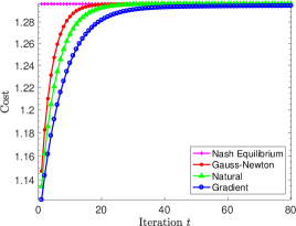
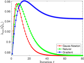
(a) $\mathcal{C}(K(L),L)$	(b) Grad. Mapp. Norm Square	(c) $\lambda_{\min}(\widetilde{Q}_{L})$

Figure 1: Performance of the three projected NG methods for Case $1$ where Assumption 2.1 ii) is satisfied. (a) shows the monotone convergence of the expected cost $\mathcal{C}(K(L),L)$ to the NE cost $\mathcal{C}(K^{*},L^{*})$; (b) shows the convergence of the gradient mapping norm square; (c) shows the change of the smallest eigenvalue of $\widetilde{Q}_{L}=Q-L^{\top}R^{v}L$.

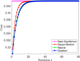
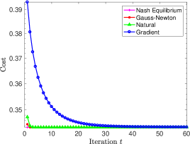
(a) Nested-Gradient	(b) Alternating-Gradient	(c) Gradient-Descent-Ascent

Figure 2: Convergence of the cost for Case $2$ where Assumption 2.1 ii) is not satisfied. (a), (b), and (c) show convergence of the NG, AG, and GDA methods, respectively.

Figure 1 shows that for Case $1$, our nested-gradient methods indeed enjoy the global convergence to the NE. The cost $\mathcal{C}(K(L),L)$ monotonically increases to that at the NE, and the convergence rate of natural NG sits between that of the other two NG methods. Also, we note that the convergence rates of gradient mapping square in (b) are linear, which are due to (c) that $\lambda(\widetilde{Q}_{L})$ is always positive along the iteration, i.e., the projection is not effective. This way, our convergence results follow from the local convergence rates in Theorem 5.3, although the initialization is random (global). We have also shown in Figure 2 that even without Assumption 2.1 ii), i.e., in Case $2$, all the PO methods mentioned successfully converge to the NE, although the cost sequences do not converge monotonically. This motivates us to provide theory for other policy optimization methods, also for more general settings of LQ games. We note that no projection was imposed when implementing these algorithms in all our experiments, which justifies that the projection here is just for the purpose of theoretical analysis. In fact, we have not found an instance of LQ games that makes the projections effective as the algorithms proceed. This motivates the theoretical study of projection-free algorithms in our future work. More simulation results can be found in §C.

8 Concluding Remarks

This paper has developed policy optimization methods, specifically, projected nested-gradient methods, to solve for the Nash equilibria of zero-sum LQ games. In spite of the nonconvexity-nonconcavity of the problem, the gradient-based algorithms have been shown to converge to the NE with globally sublinear and locally linear rates. This work appears to be the first one showing that policy optimization methods can converge to the NE of a class of zero-sum Markov games, with finite-iteration analyses. Interesting simulation results have demonstrated the superior convergence property of our algorithms, even without the projection operator, and that of the gradient-descent-ascent algorithms with simultaneous updates of both players, even when Assumption 2.1 ii) is relaxed. Based on both the theory and simulation, future directions include convergence analysis for the setting under a relaxed version of Assumption 2.1, and that for the projection-free versions of the algorithms, which we believe can be done by the techniques in our recent work Zhang et al. (2019a). Besides, developing policy optimization methods for general-sum LQ games is another interesting yet challenging future direction.

Appendix A Pseudocode for Model-Free Nested-Gradient Algorithms

In this section, we provide the pseudocode of the model-free nested-gradient algorithms, which are built upon the nested-gradient updates proposed in §4.

First, as essential elements in the nested-gradient, the gradient ${\nabla_{K}\mathcal{C}(K,L)}$ and the correlation matrix _K,L for given $K,L$ can be estimated via samples. The estimates are obtained from the function Est($K$;$L$), which is tabulated in Algorithm 1. The estimate of ${\nabla_{K}\mathcal{C}(K,L)}$, denoted by $\widehat{\nabla_{K}\mathcal{C}(K,L)}$, is obtained via zeroth-order optimization algorithms, where the perturbation $U_{i}$ is drawn from a ball with fixed radius.

Algorithm 1 Est($K$;$L$): Estimating $\widehat{\nabla_{K}\mathcal{C}(K,L)}$ and $\widehat{\Sigma}_{K,L}$ at $K$ for given $L$

1:  Input: $K,L$, number of trajectories $m$, rollout length $\mathcal{R}$, smooth parameter $r$, dimension $\widetilde{d}=m_{1}d$

2:  for $i=1,\cdots m$ do

3:     Sample a policy $\widehat{K}_{i}=K+U_{i}$, where $U_{i}$ is drawn uniformly at random over matrices with $\|U_{i}\|_{F}=r$

4:     Simulate $(\widehat{K}_{i},L)$ for $\mathcal{R}$ steps starting from $x_{0}\sim\mathcal{D}$, and collect the empirical estimates $\widehat{\mathcal{C}}_{i}$ and $\widehat{\Sigma}_{i}$ as:

$$\widehat{\mathcal{C}}_{i}=\sumop\displaylimits_{t=1}^{\mathcal{R}}c_{t}\,,\quad\widehat{\Sigma}_{i}=\sumop\displaylimits_{t=1}^{\mathcal{R}}x_{t}x_{t}^{\top}$$

where $c_{t}$ and $x_{t}$ are the costs and states following this trajectory

5:  end for

6:  Return the estimates:

$$\widehat{\nabla_{K}\mathcal{C}(K,L)}=\frac{1}{m}\sumop\displaylimits_{i=1}^{m}\frac{\widetilde{d}}{r^{2}}\widehat{\mathcal{C}}_{i}U_{i}\,,\quad\widehat{\Sigma}_{K,L}=\frac{1}{m}\sumop\displaylimits_{i=1}^{m}\widehat{\Sigma}_{i}.$$

Algorithm 2 Inner-NG($L$): Model-Free Updates For Finding $K(L)$

1:  Input: $L$, number of iterations ${\mathcal{T}}$, initialization $K_{0}$ such that $(K_{0},L)$ is stable

2:  for $\tau=0,\cdots,{\mathcal{T}}-1$ do

3:     Call Est($K_{\tau}$;$L$) to obtain the gradient and the correlation matrix estimates:

$$[\widehat{\nabla_{K}\mathcal{C}(K_{\tau},L)},\widehat{\Sigma}_{K_{\tau},L}]=\textbf{Est}(K_{\tau};L)$$

4:     Either PG update: $~{}~{}\quad\quad\quad\quad K_{\tau+1}=K_{\tau}-\alpha\widehat{\nabla_{K}\mathcal{C}(K_{\tau},L)},$or natural PG update: $\quad\qquad K_{\tau+1}=K_{\tau}-\alpha\widehat{\nabla_{K}\mathcal{C}(K_{\tau},L)}\cdot\widehat{\Sigma}_{K_{\tau},L}^{-1}.$

5:  end for

6:  Return the iterate $K_{{\mathcal{T}}}$

Given Algorithm 1, we then summarize the model-free updates for solving the inner-loop minimization problem, i.e., finding $K(L)$ as a subroutine Inner-NG($L$) in Algorithm 2. Note that among updates (4.3)-(4), only the policy gradient and the natural PG updates can be converted to model-free versions.

After a finite number ${\mathcal{T}}$ of inner-loop updates in Algorithm 2, the approximate stationary point solution $K_{{\mathcal{T}}}$ is then substituted into the outer-loop nested-gradient update, as shown in Algorithm 3. Note that the example uses projected NG update only, since the corresponding projection operator $\mathbb{P}^{GD}[\cdot]$, see definition in (4.7), does not rely on the iterate $L_{t}$ at each iteration $t$. Then after a finite number $T$ of projected NG iterates, the algorithm outputs the solution pair $\big{(}\widehat{K(L_{T})},L_{T}\big{)}$.

Algorithm 3 Outer-NG: Model-Free Nested-Gradient Algorithms

1:  Input: $L_{0}$, number of trajectories $m$, number of iterations $T$, rollout length $\mathcal{R}$, parameter $r$, dimension $\widetilde{d}=m_{2}d$

2:  for $t=0,\cdots,T-1$ do

3:     for $i=1,\cdots m$ do

4:        Sample a policy $\widehat{L}_{i}=L_{t}+V_{i}$, where $V_{i}$ is drawn uniformly at random over matrices with $\|V_{i}\|_{F}=r$

5:        Call Inner-NG($\widehat{L}_{i}$) to obtain the estimate of $K(\widehat{L}_{i})$:

$$\widehat{K(\widehat{L}_{i})}=\textbf{Inner-NG}(\widehat{L}_{i})$$

6:        Simulate $(\widehat{K(\widehat{L}_{i})},\widehat{L}_{i})$ for $\mathcal{R}$ steps starting from $x_{0}\sim\mathcal{D}$, and collect the empirical estimates $\widehat{C}_{i}$ and $\widehat{\Sigma}_{i}$ as:

$$\widehat{\mathcal{C}}_{i}=\sumop\displaylimits_{t=1}^{\mathcal{R}}c_{t}\,,\quad\widehat{\Sigma}_{i}=\sumop\displaylimits_{t=1}^{\mathcal{R}}x_{t}x_{t}^{\top}$$

where $c_{t}$ and $x_{t}$ are the costs and states following this trajectory

7:     end for

8:     Obtain the estimates of the gradient and the correlation matrix:

$$\widehat{\nabla_{L}\widetilde{\mathcal{C}}(L_{t})}=\frac{1}{m}\sumop\displaylimits_{i=1}^{m}\frac{\widetilde{d}}{r^{2}}\widehat{\mathcal{C}}_{i}V_{i}\,,\quad\widehat{\Sigma}_{\widehat{K(L_{t})},L_{t}}=\frac{1}{m}\sumop\displaylimits_{i=1}^{m}\widehat{\Sigma}_{i}$$

9:     Either projected NG update: $\quad\quad\quad\quad L_{t+1}=\mathbb{P}^{GD}\Big{[}L_{t}+\eta\widehat{\nabla_{L}\widetilde{\mathcal{C}}(L_{t})}\Big{]},$or projected natural NG update: $~{}~{}\quad\quad L_{t+1}=\mathbb{P}^{NG}\Big{[}L_{t}+\eta\widehat{\nabla_{L}\widetilde{\mathcal{C}}(L_{t})}\widehat{\Sigma}_{\widehat{K(L_{t})},L_{t}}^{-1}\Big{]}.$

10:  end for

11:  Return the iterate $L_{T}$.

Appendix B Supplementary Proofs

In this section, we provide supplementary proofs for some results that are either claimed in the paper or used in the proofs before.

B.1 Proof of Lemma 2.2

Proof.

Since $Q-(L^{*})^{\top}R^{v}L^{*}>0$, we know that $Q>0$, which implies that $(A,Q^{1/2})$ is observable. Then by Theorem $3.7$ in Başar and Bernhard (2008), the existence of $P^{*}$ in Assumption 2.1 shows that the value of the game (2.7) exists. Moreover, by Lemma $3.1$ in Stoorvogel and Weeren (1994), such a stabilizing solution $P^{*}$, if exists, is unique. Hence, by (Başar and Bernhard, 2008, Theorem $3.7$), the value of the game (2.7) is represented as $x_{0}^{\top}P^{*}x_{0}$, and given $\{u_{t}^{*}\}_{t\geq 0}$, $\{v_{t}^{*}\}_{t\geq 0}$ achieves the upper-value among any control sequence $\{v_{t}\}_{t\geq 0}$, i.e., for any $x_{0}\in\mathbb{R}^{d}$,

$$\sumop\displaylimits_{t=0}^{\infty}c_{t}(x_{t},u^{*}_{t},v_{t})\leq\sumop\displaylimits_{t=0}^{\infty}c_{t}(x_{t},u^{*}_{t},v^{*}_{t}).$$ (B.1)

Also, the closed-loop system $A-BK^{*}-CL^{*}$ is stable, i.e., the control pair $(K^{*},L^{*})$ is stabilizing.

On the other hand, by Jacobson (1977), given $\{v_{t}^{*}\}_{t\geq 0}$, $\{u_{t}^{*}\}_{t\geq 0}$ achieves the lower-value among any stabilizing control sequence $\{u_{t}\}_{t\geq 0}$; for the control sequence $\{u_{t}\}_{t\geq 0}$ that is not stabilizing, since $Q-(L^{*})^{\top}R^{v}L^{*}>0$, the cost goes to infinity. Hence,

$$\sumop\displaylimits_{t=0}^{\infty}c_{t}(x_{t},u^{*}_{t},v^{*}_{t})\leq\sumop\displaylimits_{t=0}^{\infty}c_{t}(x_{t},u_{t},v^{*}_{t}),$$ (B.2)

for any control sequence $\{u_{t}\}_{t\geq 0}$. Combining (B.1) and (B.2) yields that $(\{u_{t}^{*}\}_{t\geq 0},\{v_{t}^{*}\}_{t\geq 0})$ is a saddle-point of the game, i.e., the NE of the game (2.7), which completes the proof. ∎

B.2 Proof of Lemma 3.1

Proof.

Since by Assumption 2.1, $Q-(L^{*})^{\top}R^{v}L^{*}>0$ and $\rho(A-BK^{*}-CL^{*})<1$, it suffices to only consider those $L\in\underline{\Omega}$. For those $L$, $Q+K^{\top}R^{u}K-L^{\top}R^{v}L>0$, implying that the necessary and sufficient condition for the cost $\mathcal{C}(K,L)$ to be finite is that the control pair $(K,L)$ is stabilizing. Thus, we can use the counter-example used in the proof of Lemma $2$ in Fazel et al. (2018), by making $B=C=\mathrm{I}$, and letting $A-CL$ here equal to the $A$ matrix there, in order to show the nonconvexity of the feasible set of $K$ for these given $L$. Hence, $\min_{K}\mathcal{C}(K,L)$ is a nonconvex minimization problem. Similarly, by letting $A-BK$ and $C$ here equal to $A$ and $B$ there, respectively, we know that the set of stabilizing $L$ for these given $K$ is not convex. Therefore, $\max_{L\in\underline{\Omega}}\mathcal{C}(K,L)$ is a nonconcave maximization problem, which completes the proof. ∎

B.3 Proof of Lemma 3.2

Proof.

Let $\mathcal{C}_{K,L}(x)=x^{\top}P_{K,L}x$. Then

$$\mathcal{C}_{K,L}(x_{0})=x_{0}^{\top}(Q+K^{\top}R^{u}K-L^{\top}R^{v}L)x_{0}+\mathcal{C}_{K,L}((A-BK-CL)x_{0}).$$ (B.3)

Note that $\mathcal{C}_{K,L}((A-BK-CL)x_{0})$ on the right-hand side of (B.3) has both its subscript and the argument related to $K$. Thus, we have

$$\nabla_{K}\mathcal{C}(K,L)= ~{}2R^{u}Kx_{0}x_{0}^{\top}-2B^{\top}P_{K,L}(A-BK-CL)x_{0}x_{0}^{\top}+\nabla_{K}\mathcal{C}_{K,L}(x_{1}){\,\big{|}\,}_{x_{1}=(A-BK-CL)x_{0}}$$

$$= ~{}2[(R^{u}+B^{\top}P_{K,L}B)K-B^{\top}P_{K,L}(A-CL)]\cdot\sumop\displaylimits_{t=0}^{\infty}x_{t}x_{t}^{\top},$$

where the second equation follows from induction. Similarly, we can obtain the gradient w.r.t. $L$ as (3.5), which completes the proof. ∎

B.4 Proof of Lemma 3.3

Proof.

Since _K,L is full-rank, then if $\nabla_{K}\mathcal{C}(K,L)=\nabla_{L}\mathcal{C}(K,L)=0$, we have

$$K= ~{}(R^{u}+B^{\top}P_{K,L}B)^{-1}B^{\top}P_{K,L}(A-CL)$$ (B.4)

$$L= ~{}(-R^{v}+C^{\top}P_{K,L}C)^{-1}C^{\top}P_{K,L}(A-BK),$$ (B.5)

provided that the matrix inversion $(-R^{v}+C^{\top}P_{K,L}C)^{-1}$ exists. By solving (B.4) and (B.5), we obtain that

$$K= ~{}[R^{u}+B^{\top}P_{K,L}B-B^{\top}P_{K,L}C(-R^{v}+C^{\top}P_{K,L}C)^{-1}C^{\top}P_{K,L}B]^{-1}$$

$$\quad\times[B^{\top}P_{K,L}A-B^{\top}P_{K,L}C(-R^{v}+C^{\top}P_{K,L}C)^{-1}C^{\top}P_{K,L}A],$$ (B.6)

$$L= ~{}[-R^{v}+C^{\top}P_{K,L}C-C^{\top}P_{K,L}B(R^{u}+B^{\top}P_{K,L}B)^{-1}B^{\top}P_{K,L}C]^{-1}$$

$$\quad\times[C^{\top}P_{K,L}A-C^{\top}P_{K,L}B(R^{u}+B^{\top}P_{K,L}B)^{-1}B^{\top}P_{K,L}A].$$ (B.7)

Now it suffices to compare $P_{K,L}$ and $P^{*}$. In fact, at the NE, $P^{*}$ should also satisfy the Lyapunov equation, i.e.,

$$P^{*}=Q+(K^{*})^{\top}R^{u}K^{*}-(L^{*})^{\top}R^{v}L^{*}+(A-BK^{*}-CL^{*})^{\top}P^{*}(A-BK^{*}-CL^{*}),$$ (B.8)

where $K^{*}$ and $L^{*}$ satisfy (2.5) and (2.6). Note that the set of equations (B.6), (B.7), and (3.1) is essentially the same as the set of equations (2.5), (2.6), and (B.8). Thus, the two sets of equations have identical solutions, which are all solutions to the GARE (2.2) since the latter can be obtained by substituting (2.5) and (2.6) into (B.8).

On the other hand, under Assumption 2.1, the solution $P^{*}$ to the GARE (2.2) is unique in the regime of positive definite matrices that generate a stabilizing control pair $(K^{*},L^{*})$ following (B.6)-(B.7) (Stoorvogel and Weeren, 1994; Başar and Bernhard, 2008). Hence, such a stable control pair $(K,L)$ coincides with the NE pair $(K^{*},L^{*})$, which completes the proof. ∎

B.5 Proof of Lemma 4.1

Proof.

Recall the definition of in (4.8) for any $0<\zeta<\sigma_{\min}(\widetilde{Q}_{L^{*}})$. Then for any $L_{1},L_{2}\in\Omega$ and $\lambda\in[0,1]$, we have

$$[\lambda L_{1}+(1-\lambda)L_{2}]^{\top}R^{v}[\lambda L_{1}+(1-\lambda)L_{2}]$$

$$\quad=\lambda^{2}L_{1}^{\top}R^{v}L_{1}+(1-\lambda)^{2}L_{2}^{\top}R^{v}L_{2}+\lambda(1-\lambda)\big{(}L_{1}^{\top}R^{v}L_{2}+L_{2}^{\top}R^{v}L_{1}\big{)}$$

$$\quad\leq\lambda^{2}L_{1}^{\top}R^{v}L_{1}+(1-\lambda)^{2}L_{2}^{\top}R^{v}L_{2}+\lambda(1-\lambda)\big{(}L_{1}^{\top}R^{v}L_{1}+L_{2}^{\top}R^{v}L_{2}\big{)}$$

$$\quad\leq[\lambda^{2}+(1-\lambda)^{2}+2\lambda(1-\lambda)]\cdot(Q-\zeta\cdot\mathrm{I})=Q-\zeta\cdot\mathrm{I},$$

where the first inequality follows from $(L_{1}-L_{2})^{\top}R^{v}(L_{1}-L_{2})\geq 0$ for $R^{v}>0$, and the second inequality is by definition of $L_{1}$ and $L_{2}$. This shows that $\lambda L_{1}+(1-\lambda)L_{2}$ also lies in , which shows that the set is convex.

Moreover, since the largest eigenvalue of $L^{\top}R^{v}L-Q+\zeta\cdot\mathrm{I}$, i.e., $\lambda_{\max}(L^{\top}R^{v}L-Q+\zeta\cdot\mathrm{I})$ is a continuous function of $L$, and is lower bounded by $-\lambda_{\max}(Q)+\zeta$, the lower-level set $\{L{\,|\,}\lambda_{\max}(L^{\top}R^{v}L-Q+\zeta\cdot\mathrm{I})\leq 0\}$ is closed and bounded, i.e., compact, which proves that is compact, thus completing the proof. ∎

B.6 Proof of Lemma 6.3

Proof.

We choose the proof for the projected natural NG operator $\mathbb{P}^{NG}$ as an example. The proofs for the other two operators are similar, and follow directly. Recall that the following definition of $\mathbb{P}^{NG}$ at iterate $L$ is

$$\mathbb{P}^{NG}[\widetilde{L}]=\mathop{\mathrm{argmin}}_{\check{L}\in\Omega}~{}\mathop{\mathrm{Tr}}\Big{[}\big{(}\check{L}-\widetilde{L}\big{)}{}_{L}^{*}\big{(}\check{L}-\widetilde{L}\big{)}^{\top}\Big{]},$$

whose optimality condition can be written as

$$\mathop{\mathrm{Tr}}\Big{[}\big{(}\mathbb{P}^{NG}[\widetilde{L}]-\widetilde{L}\big{)}{}_{L}^{*}\big{(}\check{L}-\mathbb{P}^{NG}[\widetilde{L}]\big{)}^{\top}\Big{]}\geq 0,\qquad\forall\check{L}\in\Omega.$$

Letting $\widetilde{L}=L_{1}$ and $\check{L}=\mathbb{P}^{NG}[L_{2}]$, we have

$$\mathop{\mathrm{Tr}}\Big{[}\big{(}\mathbb{P}^{NG}[L_{1}]-L_{1}\big{)}{}_{L}^{*}\big{(}\mathbb{P}^{NG}[L_{2}]-\mathbb{P}^{NG}[L_{1}]\big{)}^{\top}\Big{]}\geq 0.$$ (B.9)

Also, letting $\widetilde{L}=L_{2}$ and $\check{L}=\mathbb{P}^{NG}[L_{1}]$ yields

$$\mathop{\mathrm{Tr}}\Big{[}\big{(}\mathbb{P}^{NG}[L_{2}]-L_{2}\big{)}{}_{L}^{*}\big{(}\mathbb{P}^{NG}[L_{1}]-\mathbb{P}^{NG}[L_{2}]\big{)}^{\top}\Big{]}\geq 0.$$ (B.10)

Combining (B.9) and (B.10) leads to

$$\mathop{\mathrm{Tr}}\Big{[}\big{(}L_{1}-L_{2}-\mathbb{P}^{NG}[L_{1}]+\mathbb{P}^{NG}[L_{2}]\big{)}{}_{L}^{*}\big{(}\mathbb{P}^{NG}[L_{1}]-\mathbb{P}^{NG}[L_{2}]\big{)}^{\top}\Big{]}\geq 0,$$

namely,

$$\mathop{\mathrm{Tr}}\Big{[}\big{(}L_{1}-L_{2}\big{)}{}_{L}^{*}\big{(}\mathbb{P}^{NG}[L_{1}]-\mathbb{P}^{NG}[L_{2}]\big{)}^{\top}\Big{]}\geq\mathop{\mathrm{Tr}}\Big{[}\big{(}\mathbb{P}^{NG}[L_{1}]-\mathbb{P}^{NG}[L_{2}]\big{)}{}_{L}^{*}\big{(}\mathbb{P}^{NG}[L_{1}]-\mathbb{P}^{NG}[L_{2}]\big{)}^{\top}\Big{]},$$

which completes the proof. ∎

B.7 Proof of Lemma 6.4

Proof.

Note that the Riccati equation for the inner problem (see (4.2)) can be rewritten as

$$P_{L}^{*}=\widetilde{Q}_{L}+\widetilde{A}_{L}^{\top}\big{[}I+P_{L}^{*}B(R^{u})^{-1}B^{\top}\big{]}^{-1}P_{L}^{*}\widetilde{A}_{L}.$$ (B.11)

We now use the implicit function theorem (Krantz and Parks, 2012) to show that $P_{L}^{*}$ is a continuous function of $L$. To this end, it suffices to show that $\text{vec}(P_{L}^{*})$ is continuous w.r.t. $\text{vec}(L)$.

By vectorizing both sides of (B.11), we have

$$\Psi\big{(}\text{vec}(P_{L}^{*}),\text{vec}(L)\big{)}: =\text{vec}(\widetilde{Q}_{L})+\text{vec}\big{\{}\widetilde{A}_{L}^{\top}\big{[}I+P_{L}^{*}B(R^{u})^{-1}B^{\top}\big{]}^{-1}P_{L}^{*}\widetilde{A}_{L}\big{\}}$$

$$=\text{vec}(\widetilde{Q}_{L})+\big{(}\widetilde{A}_{L}^{\top}\otimes\widetilde{A}_{L}^{\top}\big{)}\text{vec}\big{\{}\big{[}I+P_{L}^{*}B(R^{u})^{-1}B^{\top}\big{]}^{-1}P_{L}^{*}\big{\}}=\text{vec}(P_{L}^{*}),$$

where we define a mapping $\Psi:\mathbb{R}^{d^{2}}\times\mathbb{R}^{m_{2}d}\to\mathbb{R}^{d^{2}}$ as above, and also use the relationship between Kronecker product and matrix vectorization that for any matrices $A$, $B$, and $X$ with proper dimensions

$$\text{vec}(AXB)=\big{(}B^{\top}\otimes A\big{)}\text{vec}(X).$$

Then by the chain rule of matrix differentials (see Theorem $9$ in Magnus and Neudecker (1985)), we know that

$$\frac{\partial\text{vec}\big{\{}\big{[}I+P_{L}^{*}B(R^{u})^{-1}B^{\top}\big{]}^{-1}P_{L}^{*}\big{\}}}{\partial\text{vec}^{\top}(P_{L}^{*})}$$

$$\quad=(P_{L}^{*}\otimes I)\cdot\frac{\partial\text{vec}\big{\{}\big{[}I+P_{L}^{*}B(R^{u})^{-1}B^{\top}\big{]}^{-1}\big{\}}}{\partial\text{vec}^{\top}(P_{L}^{*})}+I\otimes\big{[}I+P_{L}^{*}B(R^{u})^{-1}B^{\top}\big{]}^{-1},$$ (B.12)

where $I$ denotes the identity matrices of compatible dimensions.

Now we show that

$$\frac{\partial\text{vec}\big{\{}\big{[}I+P_{L}^{*}B(R^{u})^{-1}B^{\top}\big{]}^{-1}\big{\}}}{\partial\text{vec}^{\top}(P_{L}^{*})}$$

$$\quad=\big{\{}-B(R^{u})^{-1}B^{\top}\cdot\big{[}I+P_{L}^{*}B(R^{u})^{-1}B^{\top}\big{]}^{-1}\big{\}}\otimes\big{[}I+P_{L}^{*}B(R^{u})^{-1}B^{\top}\big{]}^{-1}.$$ (B.13)

To this end, since both sides of (B.7) are matrices with dimension $d^{2}\times d^{2}$, we can compare the element at the $[(j-1)d+i]$-th row and the $[(l-1)d+k]$-th column on both sides with $i,j,k,l\in[d]$. On the left-hand side, we first notice that

$$\frac{\partial\text{vec}\big{\{}\big{[}I+P_{L}^{*}B(R^{u})^{-1}B^{\top}\big{]}^{-1}\big{\}}}{\partial[P_{L}^{*}]_{k,l}}$$

$$\quad=-\big{[}I+P_{L}^{*}B(R^{u})^{-1}B^{\top}\big{]}^{-1}\cdot\frac{\partial[P_{L}^{*}B(R^{u})^{-1}B^{\top}]}{\partial[P_{L}^{*}]_{k,l}}\cdot\big{[}I+P_{L}^{*}B(R^{u})^{-1}B^{\top}\big{]}^{-1},$$

since for some matrix function $F$, $(F^{-1})^{\prime}=-F^{-1}F^{\prime}F^{-1}$. Also, due to the fact that

$$\frac{\partial[P_{L}^{*}B(R^{u})^{-1}B^{\top}]}{\partial[P_{L}^{*}]_{k,l}}=\left[\begin{matrix}\rule[5.0pt]{60.0pt}{0.4pt}&0&\rule[5.0pt]{60.0pt}{0.4pt}\\ \big{[}B(R^{u})^{-1}B^{\top}\big{]}_{l,1}&\cdots&\big{[}B(R^{u})^{-1}B^{\top}\big{]}_{l,m}\\ \rule[2.0pt]{60.0pt}{0.4pt}&0&\rule[2.0pt]{60.0pt}{0.4pt}\end{matrix}\right]\leftarrow k\text{-th row},$$

we have

$$\Bigg{[}\frac{\partial\text{vec}\big{\{}\big{[}I+P_{L}^{*}B(R^{u})^{-1}B^{\top}\big{]}^{-1}\big{\}}}{\partial\text{vec}^{\top}(P_{L}^{*})}\Bigg{]}_{(j-1)d+i,(l-1)d+k}=\frac{\partial\Big{[}\big{[}I+P_{L}^{*}B(R^{u})^{-1}B^{\top}\big{]}^{-1}\Big{]}_{i,j}}{\partial[P_{L}^{*}]_{k,l}}$$

$$\quad=-\Big{[}\big{[}I+P_{L}^{*}B(R^{u})^{-1}B^{\top}\big{]}^{-1}\Big{]}_{i,k}\cdot\sumop\displaylimits_{q=1}^{d}\big{[}B(R^{u})^{-1}B^{\top}\big{]}_{l,q}\cdot\Big{[}\big{[}I+P_{L}^{*}B(R^{u})^{-1}B^{\top}\big{]}^{-1}\Big{]}_{q,j}.$$ (B.14)

On the right-hand side of (B.7), we have

$$\bigg{[}-\Big{\{}B(R^{u})^{-1}B^{\top}\cdot\big{[}I+P_{L}^{*}B(R^{u})^{-1}B^{\top}\big{]}^{-1}\Big{\}}\otimes\big{[}I+P_{L}^{*}B(R^{u})^{-1}B^{\top}\big{]}^{-1}\bigg{]}_{(j-1)d+i,(l-1)d+k}$$

$$\quad=\Big{[}-B(R^{u})^{-1}B^{\top}\cdot\big{[}I+P_{L}^{*}B(R^{u})^{-1}B^{\top}\big{]}^{-1}\Big{]}_{j,l}\cdot\Big{[}\big{[}I+P_{L}^{*}B(R^{u})^{-1}B^{\top}\big{]}^{-1}\Big{]}_{i,k}$$

$$\quad=\Big{[}-B(R^{u})^{-1}B^{\top}\cdot\big{[}I+P_{L}^{*}B(R^{u})^{-1}B^{\top}\big{]}^{-1}\Big{]}_{l,j}\cdot\Big{[}\big{[}I+P_{L}^{*}B(R^{u})^{-1}B^{\top}\big{]}^{-1}\Big{]}_{i,k},$$ (B.15)

where the first equation is due to the definition of Kronecker product, and the second one follows from that the matrix

$$-B(R^{u})^{-1}B^{\top}\cdot\big{[}I+P_{L}^{*}B(R^{u})^{-1}B^{\top}\big{]}^{-1}$$

$$\quad=-B(R^{u})^{-1}B^{\top}+B(R^{u})^{-1}B^{\top}\big{[}(P^{*}_{L})^{-1}+B(R^{u})^{-1}B^{\top}\big{]}^{-1}B(R^{u})^{-1}B^{\top}$$

is symmetric. Therefore, for any $(i,j,k,l)\in[d]$, (B.7) and (B.7) are identical, which verifies (B.7).

Combining (B.7) with (B.7), we have

$$\frac{\partial\text{vec}\big{\{}\big{[}I+P_{L}^{*}B(R^{u})^{-1}B^{\top}\big{]}^{-1}P_{L}^{*}\big{\}}}{\partial\text{vec}^{\top}(P_{L}^{*})}=I\otimes\big{[}I+P_{L}^{*}B(R^{u})^{-1}B^{\top}\big{]}^{-1}$$

$$\quad\qquad+(P_{L}^{*}\otimes I)\cdot\big{\{}-B(R^{u})^{-1}B^{\top}\cdot\big{[}I+P_{L}^{*}B(R^{u})^{-1}B^{\top}\big{]}^{-1}\big{\}}\otimes\big{[}I+P_{L}^{*}B(R^{u})^{-1}B^{\top}\big{]}^{-1}$$

$$\quad=\big{\{}I-P_{L}^{*}B(R^{u})^{-1}B^{\top}\cdot\big{[}I+P_{L}^{*}B(R^{u})^{-1}B^{\top}\big{]}^{-1}\big{\}}\otimes\big{[}I+P_{L}^{*}B(R^{u})^{-1}B^{\top}\big{]}^{-1}$$

$$\quad=\big{[}I+P_{L}^{*}B(R^{u})^{-1}B^{\top}\big{]}^{-1}\otimes\big{[}I+P_{L}^{*}B(R^{u})^{-1}B^{\top}\big{]}^{-1}$$ (B.16)

where the second equation uses the fact that $(A\otimes B)(C\otimes D)=(AC)\otimes(BD)$ and $(A\otimes B)+(C\otimes B)=(A+C)\otimes B$, and the last one uses matrix inversion lemma. Hence, we can write the partial derivative of $\Psi\big{(}\text{vec}(P_{L}^{*}),\text{vec}(L)\big{)}-\text{vec}(P_{L}^{*})$ as

$$\frac{\partial\big{[}\Psi\big{(}\text{vec}(P_{L}^{*}),\text{vec}(L)\big{)}-\text{vec}(P_{L}^{*})\big{]}}{\partial\text{vec}^{\top}(P_{L}^{*})}$$

$$\quad=\Big{\{}\widetilde{A}_{L}^{\top}\big{[}I+P_{L}^{*}B(R^{u})^{-1}B^{\top}\big{]}^{-1}\Big{\}}\otimes\Big{\{}\widetilde{A}_{L}^{\top}\big{[}I+P_{L}^{*}B(R^{u})^{-1}B^{\top}\big{]}^{-1}\Big{\}}-I.$$ (B.17)

By definition of $K(L)$ in (4.1), we have

$$\widetilde{A}_{L}^{\top}\big{[}I+P_{L}^{*}B(R^{u})^{-1}B^{\top}\big{]}^{-1}=\Big{\{}\widetilde{A}_{L}\big{[}I+B(R^{u})^{-1}B^{\top}P_{L}^{*}\big{]}^{-1}\Big{\}}^{\top}=\big{[}\widetilde{A}_{L}-BK(L)\big{]}^{\top}.$$

By Lemma 6.2, we know that $L\in\underline{\Omega}$ implies that $(K(L),L)$ is stabilizing, i.e., $\widetilde{A}_{L}^{\top}\big{[}I+P_{L}^{*}B(R^{u})^{-1}B^{\top}\big{]}^{-1}$ has spectral radius less than $1$. Therefore, the partial derivative in (B.7) is invertible, since the eigenvalues of the first matrix on the right-hand side of (B.7) are the products of any two eigenvalues of $\widetilde{A}_{L}^{\top}\big{[}I+P_{L}^{*}B(R^{u})^{-1}B^{\top}\big{]}^{-1}$, which have absolute values smaller than $1$. In addition, $\Psi\big{(}\text{vec}(P_{L}^{*}),\text{vec}(L)\big{)}-\text{vec}(P_{L}^{*})$ is continuous w.r.t. both $\text{vec}(P_{L}^{*})$ and $\text{vec}(L)$. Hence, we obtain from the implicit function theorem that $\text{vec}(P_{L}^{*})$ is a continuously differentiable function w.r.t. $\text{vec}(L)$, at some open neighborhood around $L$, so is $P_{L}^{*}$ w.r.t. $L$. Note that such an argument holds for any $L\in\underline{\Omega}$, which completes the proof. ∎

B.8 Proof of Lemma 6.8

Proof.

The proof is composed of several important lemmas, following the same vein as the proof of Lemma $16$ in Fazel et al. (2018). Note that Assumption 2.1 is assumed to hold throughout the proof, and will not be repeated at each intermediate result.

We first provide the perturbation result for $P_{L}^{*}$ in the following proposition. The results are based on the perturbation theory of algebraic Riccati equations in Konstantinov et al. (1993); Sun (1998), since for given $L$, $P_{L}^{*}$ is the solution to the inner-loop Riccati equation (4.2) with cost matrix $\widetilde{Q}_{L}=Q-L^{\top}R^{v}L$ and transition matrix $\widetilde{A}_{L}=A-CL$.

Proposition B.1 (Perturbation of $P_{L}^{*}$).

For any $L,L^{\prime}\in\Omega$, where is defined in (4.8), there exists some constant $\mathcal{B}^{L}>0$ such that if $\|L^{\prime}-L\|\leq\mathcal{B}^{L},$ it follows that

$$\|P_{L^{\prime}}^{*}-P_{L}^{*}\|\leq\mathcal{B}^{P}\cdot\|L^{\prime}-L\|,$$

for some constant $\mathcal{B}^{P}>0$.

Proof.

The proof is built upon the result of Theorem $4.1$ in Sun (1998). First, since both $L,L^{\prime}\in\Omega$, we have $\widetilde{Q}_{L^{\prime}},\widetilde{Q}_{L}\geq 0$, and also $B(R^{u})^{-1}B^{\top}\geq 0$ for both $L$ and $L^{\prime}$. This validates the applicability of (Sun, 1998, Theorem $4.1$). Also note that by Lemma 6.2, both $P_{L}^{*}$ and $P_{L^{\prime}}^{*}$ exist and are positive definite. First recalling the definition of $K(L)$ in (4.1), we have the following relationship:

$$\widetilde{A}_{L}-BK(L)=\widetilde{A}_{L}-B(R^{u}+B^{\top}P_{L}^{*}B)^{-1}B^{\top}P_{L}^{*}\widetilde{A}_{L}=[\mathrm{I}+B(R^{u})^{-1}B^{\top}P_{L}^{*}]^{-1}\widetilde{A}_{L},$$

where the second equation uses the matrix inversion lemma.

To simplify the notation, we let $\Delta=L^{\prime}-L$ and also define the following quantities:

$$\delta=\big{\|}\widetilde{A}_{L^{\prime}}-\widetilde{A}_{L}\big{\|}=\|C\Delta\|,\quad f=\big{\|}[\mathrm{I}+B(R^{u})^{-1}B^{\top}P_{L}^{*}]^{-1}\big{\|},\quad g=\|B(R^{u})^{-1}B^{\top}\|$$

$$\phi=\big{\|}[\mathrm{I}+B(R^{u})^{-1}B^{\top}P_{L}^{*}]^{-1}\widetilde{A}_{L}\big{\|},\quad\gamma=f\delta(2\phi+f\delta),\quad\psi=\big{\|}P_{L}^{*}\cdot[\mathrm{I}+B(R^{u})^{-1}B^{\top}P_{L}^{*}]^{-1}\big{\|}$$

$$T_{L}=\mathrm{I}-\big{[}\widetilde{A}_{L}-BK(L)\big{]}^{\top}\otimes\big{[}\widetilde{A}_{L}-BK(L)\big{]}^{\top},~{}\ell=\|T_{L}^{-1}\|^{-1},~{}H=P_{L}^{*}[\mathrm{I}+B(R^{u})^{-1}B^{\top}P_{L}^{*}]^{-1}\widetilde{A}_{L}$$

$$p=\big{\|}T_{L}^{-1}\big{[}\mathrm{I}\otimes H^{\top}+(H^{\top}\otimes\mathrm{I})\Pi\big{]}\big{\|},~{}~{}\varepsilon=\frac{1}{\ell}\big{\|}\Delta R^{v}L+L^{\top}R^{v}\Delta+{}^{\top}R^{v}\Delta\big{\|}+\Big{(}p+\frac{\psi\delta}{\ell}\Big{)}\|C\Delta\|$$

$$\qquad\qquad\qquad\qquad\qquad\alpha=f(\|\widetilde{A}_{L}\|+\|C\Delta\|),\qquad\theta=\frac{\ell}{\phi+\sqrt{\phi^{2}+\ell}},$$

where is the vec-permutation matrix (Graham, 2018, pp. 32-34). Also, from Lemma 6.2, we know that $\widetilde{A}_{L}-BK(L)$ is stabilizing, which thus implies that $\ell$ is finite and

$$\ell=1/\|T_{L}^{-1}\|=\sigma_{\min}(T_{L})>0.$$ (B.18)

We note that since is a compact set of $L$, and $\sigma_{\min}(T_{L})$ is a continuous function of $L$, $\ell$ is uniformly lower bounded above zero for any $L\in\Omega$.

Since the term $\|\Delta G\|$ in (Sun, 1998, Theorem $4.1$) is zero here, the first condition in (4.40) of Sun (1998) is trivially satisfied. For the other two conditions in (4.40) there, we require the following sufficient conditions to hold

$$1-fg\xi_{*}\geq 0,\quad\frac{f\delta+\phi fg\xi_{*}}{1-fg\xi_{*}}\leq\theta,$$ (B.19)

where $\xi_{*}$ is d efined as $\xi_{*}={(2\ell\varepsilon)}\cdot{(\ell/2+\ell fg\varepsilon)^{-1}}.$ Note that if we additionally require

$$\gamma=f\delta(2\phi+f\delta)\leq f\|C\Delta\|(2\phi+2\ell+f\|C\Delta\|)\leq 2f(\phi+\ell)\|C\|\|\Delta\|+f^{2}\|C\|^{2}\|\Delta\|^{2}\leq\ell/2,$$ (B.20)

then the definition of $\xi_{*}$ here is strictly larger than that in Sun (1998). Thus, if such an $\xi_{*}$ satisfies (B.19), then the other two conditions in (B.19) can be satisfied, too. Moreover, if we also let

$$\varepsilon =\frac{1}{\ell}\big{\|}\Delta R^{v}L+L^{\top}R^{v}\Delta+{}^{\top}R^{v}\Delta\big{\|}+\Big{(}p+\frac{\psi\delta}{\ell}\Big{)}\|C\Delta\|$$

$$\leq\frac{1}{\ell}\big{(}2\|R^{v}L\|\|\Delta\|+\|R^{v}\|\|\Delta\|^{2}\big{)}+\Big{(}p+\frac{\psi\delta}{\ell}\Big{)}\|C\Delta\|\leq\frac{(\ell/2)^{2}}{2\ell fg(\ell+2{\alpha})}=\frac{\ell}{8fg(\ell+2{\alpha})}$$ (B.21)

hold, then since $\gamma\leq\ell/2$ from (B.20), the right-hand side of (B.8) satisfies

$$\frac{(\ell/2)^{2}}{2\ell fg(\ell+2{\alpha})}\leq\frac{(\ell-\gamma)^{2}}{\ell fg(\ell-\gamma+2\alpha+\sqrt{(\ell-\gamma+2\alpha)^{2}-(\ell-\gamma)^{2}}}.$$

This implies that the condition in (4.41) in Sun (1998) holds. Then, we obtain from Theorem $4.1$ in Sun (1998) that

$$\big{\|}P_{L^{\prime}}^{*}-P_{L}^{*}\big{\|}\leq\xi_{*}=\frac{2\ell\varepsilon}{\ell/2+\ell fg\varepsilon}\leq 4\varepsilon=\frac{4}{\ell}\big{\|}\Delta R^{v}L+L^{\top}R^{v}\Delta+{}^{\top}R^{v}\Delta\big{\|}+4\Big{(}p+\frac{\psi\delta}{\ell}\Big{)}\|C\Delta\|$$

$$\quad\leq\frac{8}{\ell}\|R^{v}L\|\|\Delta\|+\frac{4}{\ell}\|R^{v}\|\|\Delta\|^{2}+4p\|C\|\|\Delta\|+4\frac{\psi}{\ell}\|C\|^{2}\|\Delta\|^{2}.$$ (B.22)

Now we discuss sufficient conditions of (B.19), (B.20), and (B.8), to ensure a perturbation bound on $P_{L}^{*}$ as desired from (B.8). The two conditions in (B.19) can be written as

$$fg\frac{2\varepsilon}{1/2+fg\varepsilon}\leq 1\Longrightarrow fg\varepsilon\leq 1/2,\quad f\delta+\big{(}\phi+\theta\big{)}fg\xi_{*}\leq\theta,$$ (B.23)

where one sufficient condition for the second one to hold is

$$f\delta+4(\phi+\theta)fg\varepsilon\leq\theta,$$ (B.24)

since $\xi_{*}\leq 2\varepsilon/(1/2)=4\varepsilon$. Note that since $f\delta\geq 0$ and $fg\varepsilon\geq 0$, (B.24) holds implies that $fg\varepsilon\leq 1/2$. Hence we only need a sufficient condition for (B.24) to hold, which can be the following one

$$f\|C\|\|\Delta\|+4(\phi+\theta)fg\bigg{(}\frac{2}{\ell}\|R^{v}L\|\|\Delta\|+\frac{1}{\ell}\|R^{v}\|\|\Delta\|^{2}+p\|C\|\|\Delta\|+\frac{\psi}{\ell}\|C\|^{2}\|\Delta\|^{2}\bigg{)}\leq\theta.$$ (B.25)

(B.25) can be satisfied if the following condition on $\|\Delta\|$ holds:

$$\|\Delta\|\leq\min\bigg{\{}\frac{\|C\|+4(\phi+\theta)g(2\|R^{v}L\|/\ell+p\|C\|)}{4(\phi+\theta)g(\|R^{v}\|/\ell+\psi\|C\|^{2}/\ell)},\frac{\theta}{2f\|C\|+8f(\phi+\theta)g(2\|R^{v}L\|/\ell+p\|C\|)}\bigg{\}}.$$ (B.26)

Moreover, the condition in (B.20) gives

$$2f(\phi+\ell)\|C\|\|\Delta\|+f^{2}\|C\|^{2}\|\Delta\|^{2}\leq\ell/2,$$ (B.27)

which can be satisfied by the following condition on $\|\Delta\|$:

$$\|\Delta\|\leq\min\bigg{\{}\frac{2(\phi+\ell)}{f\|C\|},\frac{\ell}{8f(\phi+\ell)\|C\|}\bigg{\}}.$$ (B.28)

Also, by letting

$$2\alpha=2f(\|\widetilde{A}_{L}\|+\|C\Delta\|)\leq 2f(\|\widetilde{A}_{L}\|+\|C\|)$$ (B.29)

$$\Longrightarrow\frac{\ell}{8fg(\ell+2{\alpha})}\geq\frac{\ell}{8fg[\ell+2f(\|\widetilde{A}_{L}\|+\|C\|)]},$$

the condition in (B.8) can thus be satisfied if we let

$$\frac{1}{\ell}\big{(}2\|R^{v}L\|\|\Delta\|+\|R^{v}\|\|\Delta\|^{2}\big{)}+(p+1)\|C\|\|\Delta\|+\frac{\psi}{\ell}\|C\|^{2}\|\Delta\|^{2}\leq\frac{\ell}{8fg[\ell+2f(\|\widetilde{A}_{L}\|+\|C\|)]}.$$ (B.30)

Note that conditions (B.29)-(B.30) can be satisfied if

$$\|\Delta\|\leq\min\bigg{\{}1,\frac{2\|R^{v}L\|+(p+1)\ell\|C\|}{\|R^{v}\|+\psi\|C\|^{2}},\frac{\ell}{16fg[\ell+2f(\|\widetilde{A}_{L}\|+\|C\|)](\|R^{v}L\|/\ell+2(p+1)\|C\|)}\bigg{\}}.$$ (B.31)

Thus, under (B.26), (B.28), and (B.31), the bound (B.8) can be further written as

$$\big{\|}P_{L^{\prime}}^{*}-P_{L}^{*}\big{\|}\leq\bigg{[}\frac{\|C\|}{(\phi+\theta)g}+\frac{16\|R^{v}L\|}{\ell}+8p\|C\|\bigg{]}\cdot\|\Delta\|,$$ (B.32)

where the inequality follows by using the first bound of in the $\min$ of (B.26). It is straightforward to see that all the upper bounds on $\|\Delta\|$ from (B.26), (B.28), and (B.31) are lower bounded above zero, since: i) $\ell$, $\theta$ and $\|C\|$ are all strictly above zero (see (B.18)), so are all the numerators of the bounds in (B.26), (B.28), and (B.31); ii) the denominators of the bounds are all finite and bounded above, due to the boundedness of $L$, i.e., the boundedness of , and the boundedness of $P_{L}^{*}$ from Lemma 6.2. In addition, note that all the quantities used in the bounds on $\|\Delta\|$ are norms of matrices composed of $L$ and $P_{L}^{*}$, which are both continuous functions of $L$ (see Lemma 6.4 on the continuity of $P_{L}^{*}$), over the compact set . Hence, there exists some constant $\mathcal{B}^{L}>0$, which is the infimum of the bounds on $\|\Delta\|$ over . Also, from (B.32), there exists some

$$\mathcal{B}^{P}=\frac{\|C\|}{(\phi+\theta)g}+\frac{16\|R^{v}L\|}{\ell}+8p\|C\|,$$

such that $\|P_{L^{\prime}}^{*}-P_{L}^{*}\|\leq\mathcal{B}^{P}\cdot\|L^{\prime}-L\|$, which completes the proof. ∎

We then need to establish the perturbation of $K(L)$ as in the following lemma.

Lemma B.2.

For any $L,L^{\prime}\in\Omega$, recalling the definition of $K(L)$ in (4.1), there exists some constant $\mathcal{B}^{L}>0$ such that if

$$\|L^{\prime}-L\|\leq\min\bigg{\{}\mathcal{B}^{L},\frac{\|B\|\cdot(\mathcal{B}^{P}\|\widetilde{A}_{L}-BK(L)\|+\|P_{L}^{*}\|\|C\|)}{\mathcal{B}^{P}\|B\|\|C\|}\bigg{\}},$$ (B.33)

it follows that

$$\|K(L^{\prime})-K(L)\|\leq\frac{2\|B\|\cdot(\mathcal{B}^{P}\|\widetilde{A}_{L}-BK(L)\|+\|P_{L}^{*}\|\|C\|)}{\sigma_{\min}(R^{u})}\cdot\|L^{\prime}-L\|,$$

where $\mathcal{B}^{L},\mathcal{B}^{P}$ are as defined in the proof of Proposition B.1.

Proof.

By definition, it holds that

$$(R^{u}+B^{\top}P_{\widetilde{L}}^{*}B)K(\widetilde{L})=B^{\top}P_{\widetilde{L}}^{*}\widetilde{A}_{\widetilde{L}}$$

for both $\widetilde{L}=L$ and $\widetilde{L}=L^{\prime}$. Subtracting both equations yields

$$B^{\top}(P_{L^{\prime}}^{*}-P_{L}^{*})BK(L)+(R^{u}+B^{\top}P_{L^{\prime}}B)[K(L^{\prime})-K(L)]=B^{\top}(P_{L^{\prime}}^{*}-P_{L}^{*})\widetilde{A}_{L^{\prime}}+B^{\top}P_{L}^{*}C(L-L^{\prime}),$$

which further gives

$$\|K(L^{\prime})-K(L)\|=\|(R^{u}+B^{\top}P_{L^{\prime}}B)^{-1}B^{\top}(P_{L^{\prime}}^{*}-P_{L}^{*})[\widetilde{A}_{L}-BK(L)+C(L-L^{\prime})]$$

$$\qquad\qquad\qquad\qquad\qquad+(R^{u}+B^{\top}P_{L^{\prime}}B)^{-1}B^{\top}P_{L}^{*}C(L-L^{\prime})\|$$

$$\leq\|(R^{u}+B^{\top}P_{L^{\prime}}B)^{-1}\|\|B\|\big{[}\|P_{L^{\prime}}^{*}-P_{L}^{*}\|\big{(}\|\widetilde{A}_{L}-BK(L)\|+\|C\|\|L^{\prime}-L\|\big{)}+\|P_{L}^{*}\|\|C\|\|L^{\prime}-L\|\big{]}$$

$$\leq\frac{\|B\|}{\sigma_{\min}(R^{u})}\|P_{L^{\prime}}^{*}-P_{L}^{*}\|\big{(}\|\widetilde{A}_{L}-BK(L)\|+\|C\|\|L^{\prime}-L\|\big{)}+\frac{\|B\|}{\sigma_{\min}(R^{u})}\|P_{L}^{*}\|\|C\|\|L^{\prime}-L\|.$$

Combined with the bound on $\|P_{L^{\prime}}^{*}-P_{L}^{*}\|$ in Proposition B.1, we obtain that

$$\|K(L^{\prime})-K(L)\|\leq\frac{\|B\|\cdot(\mathcal{B}^{P}\|\widetilde{A}_{L}-BK(L)\|+\|P_{L}^{*}\|\|C\|)}{\sigma_{\min}(R^{u})}\|L^{\prime}-L\|+\frac{\mathcal{B}^{P}\|B\|\|C\|}{\sigma_{\min}(R^{u})}\|L^{\prime}-L\|^{2},$$

which combined with the bound on (B.33) gives the desired result. ∎

Now we are ready to establish the perturbation of ${}_{L}^{*}$. We start by defining a linear operator on symmetric matrices ${\mathcal{T}}_{L}^{*}(\cdot)$:

$${\mathcal{T}}_{L}^{*}(X):=\sumop\displaylimits_{t=0}^{\infty}[A-BK(L)-CL]^{t}X[A-BK(L)-CL]^{t^{\top}},$$

and its induced norm as

$$\|{\mathcal{T}}_{L}^{*}\|:=\sup_{X}\frac{{\mathcal{T}}_{L}^{*}(X)}{\|X\|},$$

where $\sup$ is taken over all non-zero symmetric matrices. Also, we let ${}_{0}=\mathbb{E}(x_{0}x_{0}^{\top})$. Then we can show that the induced norm $\|{\mathcal{T}}_{L}^{*}\|$ is bounded as follows.

Lemma B.3.

For any $L\in\Omega$, the induced norm pf $\|{\mathcal{T}}_{L}^{*}\|$ is bounded as

$$\|{\mathcal{T}}_{L}^{*}\|\leq\frac{\mathcal{C}(K(L),L)}{\mu\cdot\zeta}.$$

Proof.

The proof mostly follows the proof of Lemma $17$ in Fazel et al. (2018), except replacing $(A-BK)$ there by $A-BK(L)-CL$, and the upper bound of $\|{}_{L}^{*}\|$ by $\mathcal{C}(K(L),L)/\zeta$ due to Lemma 6.6. ∎

We can also define another operator $\mathcal{F}_{L}^{*}(X)$ as

$$\mathcal{F}_{L}^{*}(X)=[A-BK(L)-CL]X[A-BK(L)-CL]^{\top},$$

which, by the same argument as Lemma $18$ in Fazel et al. (2018), gives that

$${\mathcal{T}}_{L}^{*}=(\mathrm{I}-\mathcal{F}_{L}^{*})^{-1},$$ (B.34)

where $\mathrm{I}$ is the identity operator. Hence, the following proof is to find the bound of

$$\|{}_{L^{\prime}}^{*}-{}_{L}^{*}\|=\|({\mathcal{T}}_{L^{\prime}}^{*}-{\mathcal{T}}_{L}^{*})({}_{0})\|=\|[(\mathrm{I}-\mathcal{F}_{L^{\prime}}^{*})^{-1}-(\mathrm{I}-\mathcal{F}_{L}^{*})^{-1}]({}_{0})\|.$$

To this end, we first have the following bound on $\|\mathcal{F}_{L}^{*}-\mathcal{F}_{L^{\prime}}^{*}\|$.

Lemma B.4.

For any $L,L^{\prime}\in\Omega$, it follows that

$$\|\mathcal{F}_{L^{\prime}}^{*}-\mathcal{F}_{L}^{*}\|\leq 2\|A-BK(L)-CL\|\big{(}\|B\|\|K(L^{\prime})-K(L)\|+\|C\|\|\Delta\|\big{)}$$

$$\qquad\qquad\quad\quad+\|B\|^{2}\|K(L^{\prime})-K(L)\|^{2}+\|C\|^{2}\|\Delta\|^{2}+2\|B\|\|C\|\|K(L^{\prime})-K(L)\|\|\Delta\|.$$

Proof.

Let $\Delta=L^{\prime}-L$, then for any symmetric matrix $X$,

$$(\mathcal{F}_{L^{\prime}}^{*}-\mathcal{F}_{L}^{*})(X)= -[A-BK(L)-CL]X\big{\{}B[K(L^{\prime})-K(L)]+C\Delta\big{\}}^{\top}$$

$$\quad-\big{\{}B[K(L^{\prime})-K(L)]+C\Delta\big{\}}X[A-BK(L)-CL]^{\top}$$

$$\quad+\big{\{}B[K(L^{\prime})-K(L)]+C\Delta\big{\}}X\big{\{}B[K(L^{\prime})-K(L)]+C\Delta\big{\}}^{\top},$$

which leads to the desired norm bound by using $\|AX\|\leq\|A\|\|X\|$ for any operator $A$. ∎

Moreover, we have the following argument similar to Lemma $20$ in Fazel et al. (2018).

Lemma B.5.

If $\|{\mathcal{T}}_{L}^{*}\|\|\mathcal{F}_{L^{\prime}}^{*}-\mathcal{F}_{L}^{*}\|\leq 1/2$, and both $(K(L^{\prime}),L^{\prime})$ and $(K(L),L)$ are stabilizing. Then

$$\|({\mathcal{T}}_{L^{\prime}}^{*}-{\mathcal{T}}_{L}^{*})(\Sigma)\|\leq 2\|{\mathcal{T}}_{L}^{*}\|\|\mathcal{F}_{L^{\prime}}^{*}-\mathcal{F}_{L}^{*}\|\|{\mathcal{T}}_{L}^{*}(\Sigma)\|\leq 2\|{\mathcal{T}}_{L}^{*}\|^{2}\|\mathcal{F}_{L^{\prime}}^{*}-\mathcal{F}_{L}^{*}\|\|\Sigma\|.$$

Proof.

The proof follows directly from that of Lemma $20$ in Fazel et al. (2018), which is omitted here for brevity. ∎

We are now ready to prove the perturbation of ${}_{L}^{*}$. To simplify the notation, let

$$\mathcal{B}^{K}=\frac{2\|B\|\cdot\big{(}\mathcal{B}^{P}\|\widetilde{A}_{L}-BK(L)\|+\|P_{L}^{*}\|\|C\|\big{)}}{\sigma_{\min}(R^{u})},$$

then $\mathcal{B}^{K}>0$. By Lemmas B.2 and B.4, for any $L,L^{\prime}\in\Omega$, letting $\Delta=L^{\prime}-L$, if

$$\|\Delta\|\leq\min\Bigg{\{}\mathcal{B}^{L},\frac{\|B\|\big{[}\mathcal{B}^{P}\|\widetilde{A}_{L}-BK(L)\|+\|P_{L}^{*}\|\|C\|\big{]}}{\mathcal{B}^{P}\|B\|\|C\|},\frac{2\big{(}\|\widetilde{A}_{L}-BK(L)\|+1\big{)}\big{(}\mathcal{B}^{K}\|B\|+\|C\|\big{)}}{\big{(}\mathcal{B}^{K}\big{)}^{2}\|B\|^{2}+\|C\|^{2}+2\mathcal{B}^{K}\|B\|\|C\|}\Bigg{\}},$$

then

$$\|\mathcal{F}_{L^{\prime}}^{*}-\mathcal{F}_{L}^{*}\|\leq 2\|\widetilde{A}_{L}-BK(L)\|\big{(}\mathcal{B}^{K}\|B\|\|\Delta\|+\|C\|\|\Delta\|\big{)}$$

$$\qquad\qquad\qquad\qquad+\big{(}\mathcal{B}^{K}\big{)}^{2}\|B\|^{2}\|\Delta\|^{2}+\|C\|^{2}\|\Delta\|^{2}+2\|B\|\|C\|\mathcal{B}^{K}\|\Delta\|^{2}$$

$$\quad\leq 2\big{(}\|\widetilde{A}_{L}-BK(L)\|+1\big{)}\big{(}\mathcal{B}^{K}\|B\|\|\Delta\|+\|C\|\|\Delta\|\big{)}$$

$$\qquad\qquad\qquad\qquad+\big{(}\mathcal{B}^{K}\big{)}^{2}\|B\|^{2}\|\Delta\|^{2}+\|C\|^{2}\|\Delta\|^{2}+2\|B\|\|C\|\mathcal{B}^{K}\|\Delta\|^{2}$$

$$\quad\leq 4\big{(}\|\widetilde{A}_{L}-BK(L)\|+1\big{)}\big{(}\mathcal{B}^{K}\|B\|+\|C\|\big{)}\cdot\|\Delta\|,$$

where the first inequality uses Lemma B.2, and the second inequality is due to the third term in the $\min$ of the upper bound on $\|\Delta\|$. This completes the proof of Lemma 6.8. ∎

Lemma B.6.

For any disjoint sets $\mathcal{A},\mathcal{B}\subseteq\mathbb{R}^{m\times n}$, if $\mathcal{A}$ is compact, and if $\mathcal{B}$ is closed, then there exists some $\omega>0$, such that for any $A\in\mathcal{A}$ and $B\in\mathcal{B}$, $\|A-B\|\geq\omega$.

Proof.

Assume that the conclusion does not hold. Let $A_{n}\in\mathcal{A}$ and $B_{n}\in\mathcal{B}$ be chosen such that $\|A_{n}-B_{n}\|\to 0$ as $n\to\infty$. Since $\mathcal{A}$ is compact, there exists a convergent subsequence of $\{A_{n}\}_{n\geq 0}$, denoted by $\{A_{n_{m}}\}_{m\geq 0}$, that converges to some $A\in\mathcal{A}$. Hence, we have

$$\|A-B_{n_{m}}\|\leq\|A-A_{n_{m}}\|+\|A_{n_{m}}-B_{n_{m}}\|\to 0,$$

as $m\to\infty$. This implies that $A$ is a limit point of $\mathcal{B}$. Since $\mathcal{B}$ is closed, we have $A\in\mathcal{B}$, which leads to a contradiction and thus completes the proof. ∎

Appendix C Simulation Details

Alternating-Gradient (AG) Methods.

AG methods follows the idea in Nouiehed et al. (2019), which are based on our nested-gradient methods, but at each outer-loop iteration, the inner-loop updates only perform a finite number of iterations, instead of converging to the exact solution $K(L_{t})$ as nested-gradient methods. The updates are given in Algorithm 4, whose performance is showcased in Figures 3 and 4, showing that AG methods converge to the NE in both settings.

Algorithm 4 Alternating-Gradient (AG) Methods

1:  Input: $(K_{0},L_{0})$ that is stabilizing

2:  for $t=0,\cdots,T-1$ do

3:     for $\tau=0,\cdots{\mathcal{T}}-1$ do

4:        

$${\rm\textbf{Policy Gradient:}}\qquad~{}~{}K_{\tau+1} =K_{\tau}-\eta\nabla_{K}{\mathcal{C}}(K_{\tau},L_{t}),$$

5:        Or

$${\rm\textbf{Natural Policy Gradient:}}\qquad~{}~{}K_{\tau+1} =K_{\tau}-\eta\nabla_{K}{\mathcal{C}}(K_{\tau},L_{t}){}^{-1}_{K_{\tau},L_{t}},$$

6:        Or

$${\rm\textbf{Gauss-Newton:}}\qquad~{}~{}K_{\tau+1} =K_{\tau}-\eta(R^{u}+B^{\top}P_{K_{\tau},L_{t}}B)^{-1}\nabla_{K}{\mathcal{C}}(K_{\tau},L_{t}){}^{-1}_{K_{\tau},L_{t}},$$

7:     end for

8:     

$${\rm\textbf{Policy Gradient:}}\qquad~{}~{}L_{t+1} =L_{t}+\eta\nabla_{L}{\mathcal{C}}(K_{{\mathcal{T}}},L_{t}),$$

9:     Or

$${\rm\textbf{Natural Policy Gradient:}}\qquad~{}~{}L_{t+1} =L_{t}+\eta\nabla_{L}{\mathcal{C}}(K_{{\mathcal{T}}},L_{t}){}^{-1}_{K_{{\mathcal{T}}},L_{t}},$$

10:     Or

$${\rm\textbf{Gauss-Newton:}}\qquad~{}~{}L_{t+1} =L_{t}+\eta(R^{v}-C^{\top}P_{K_{{\mathcal{T}}},L_{t}}C)^{-1}\nabla_{L}{\mathcal{C}}(K_{{\mathcal{T}}},L_{t}){}^{-1}_{K_{{\mathcal{T}}},L_{t}},$$

11:  end for

12:  Return the iterate $(K_{{\mathcal{T}}},L_{T})$.

Algorithm 5 Gradient-Descent-Ascent (GDA) Methods

1:  Input: $(K_{0},L_{0})$ that is stabilizing

2:  for $t=0,\cdots,T-1$ do

3:     

$${\rm\textbf{Policy Gradient:}}\qquad~{}~{}K_{t+1} =K_{t}-\eta\nabla_{K}{\mathcal{C}}(K_{t},L_{t})$$

$$L_{t+1} =L_{t}+\eta\nabla_{L}{\mathcal{C}}(K_{t},L_{t}),$$

4:     Or

$${\rm\textbf{Natural Policy Gradient:}}\qquad~{}~{}K_{t+1} =K_{t}-\eta\nabla_{K}{\mathcal{C}}(K_{t},L_{t}){}^{-1}_{K_{t},L_{t}}$$

$$L_{t+1} =L_{t}+\eta\nabla_{L}{\mathcal{C}}(K_{t},L_{t}){}^{-1}_{K_{t},L_{t}},$$

5:     Or

$${\rm\textbf{Gauss-Newton:}}\qquad~{}~{}K_{t+1} =K_{t}-\eta(R^{u}+B^{\top}P_{K_{t},L_{t}}B)^{-1}\nabla_{K}{\mathcal{C}}(K_{t},L_{t}){}^{-1}_{K_{t},L_{t}}$$

$$L_{t+1} =L_{t}+\eta(R^{v}-C^{\top}P_{K_{t},L_{t}}C)^{-1}\nabla_{L}{\mathcal{C}}(K_{t},L_{t}){}^{-1}_{K_{t},L_{t}},$$

6:  end for

7:  Return the iterate $(K_{T},L_{T})$.

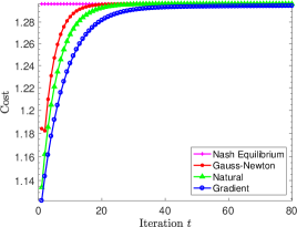
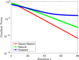
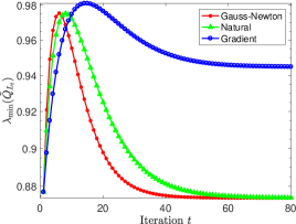
(a) $\mathcal{C}(K(L),L)$	(b) Grad. Mapp. Norm Square	(c) $\lambda_{\min}(\widetilde{Q}_{L})$

Figure 3: Performance of the three AG methods for Case $1$ where Assumption 2.1 ii) is satisfied. (a) shows the monotone convergence of the expected cost $\mathcal{C}(K(L),L)$ to the NE cost $\mathcal{C}(K^{*},L^{*})$; (b) shows the convergence of the gradient mapping norm square; (c) shows the change of the smallest eigenvalue of $\widetilde{Q}_{L}=Q-L^{\top}R^{v}L$.

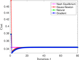
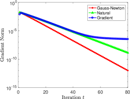
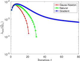
(a) $\mathcal{C}(K(L),L)$	(b) Grad. Mapp. Norm Square	(c) $\lambda_{\min}(\widetilde{Q}_{L})$

Figure 4: Performance of the three AG methods for Case $2$ where Assumption 2.1 ii) is not satisfied. (a) shows the monotone convergence of the expected cost $\mathcal{C}(K(L),L)$ to the NE cost $\mathcal{C}(K^{*},L^{*})$; (b) shows the convergence of the gradient mapping norm square; (c) shows the change of the smallest eigenvalue of $\widetilde{Q}_{L}=Q-L^{\top}R^{v}L$.

Gradient-Descent-Ascent (GDA) Methods.

Note that GDA and its variants with simultaneous updates have drawn increasing attention recently for solving saddle-point problems (Cherukuri et al., 2017; Daskalakis and Panageas, 2018; Mazumdar et al., 2019; Jin et al., 2019), mainly due to their popularity in training GANs. The algorithms perform policy gradient descent for the minimizer and ascent for the maximizer. The updates are given in Algorithm 5, whose performance is showcased in Figures 5 and 6, showing their convergence to the NE in both settings.

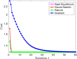
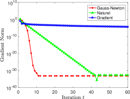
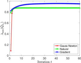
(a) $\mathcal{C}(K(L),L)$	(b) Grad. Mapp. Norm Square	(c) $\lambda_{\min}(\widetilde{Q}_{L})$

Figure 5: Performance of the three GDA methods for Case $1$ where Assumption 2.1 ii) is satisfied. (a) shows the monotone convergence of the expected cost $\mathcal{C}(K(L),L)$ to the NE cost $\mathcal{C}(K^{*},L^{*})$; (b) shows the convergence of the gradient mapping norm square; (c) shows the change of the smallest eigenvalue of $\widetilde{Q}_{L}=Q-L^{\top}R^{v}L$.

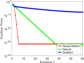
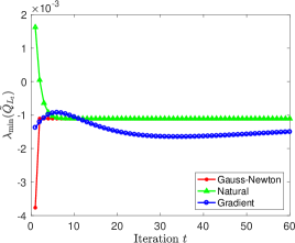
(a) $\mathcal{C}(K(L),L)$	(b) Grad. Mapp. Norm Square	(c) $\lambda_{\min}(\widetilde{Q}_{L})$

Figure 6: Performance of the three GDA methods for Case $2$ where Assumption 2.1 ii) is not satisfied. (a) shows the monotone convergence of the expected cost $\mathcal{C}(K(L),L)$ to the NE cost $\mathcal{C}(K^{*},L^{*})$; (b) shows the convergence of the gradient mapping norm square; (c) shows the change of the smallest eigenvalue of $\widetilde{Q}_{L}=Q-L^{\top}R^{v}L$.

References

- Adolphs et al. (2019) Adolphs, L., Daneshmand, H., Lucchi, A. and Hofmann, T. (2019). Local saddle point optimization: A curvature exploitation approach.
- Al-Tamimi et al. (2007) Al-Tamimi, A., Lewis, F. L. and Abu-Khalaf, M. (2007). Model-free Q-learning designs for linear discrete-time zero-sum games with application to -infinity control. Automatica, 43 473–481.
- Balduzzi et al. (2018) Balduzzi, D., Racaniere, S., Martens, J., Foerster, J., Tuyls, K. and Graepel, T. (2018). The mechanics of n-player differentiable games. In International Conference on Machine Learning.
- Banerjee and Peng (2003) Banerjee, B. and Peng, J. (2003). Adaptive policy gradient in multiagent learning. In Conference on Autonomous Agents and Multiagent Systems. ACM.
- Başar and Bernhard (2008) Başar, T. and Bernhard, P. (2008). Optimal Control and Related Minimax Design Problems: A Dynamic Game Approach. Springer Science & Business Media.
- Bertsekas (2005) Bertsekas, D. P. (2005). Dynamic Programming and Optimal Control, vol. 1. Athena Scientific Belmont, MA.
- Bowling and Veloso (2001) Bowling, M. and Veloso, M. (2001). Rational and convergent learning in stochastic games. In International Joint Conference on Artificial Intelligence, vol. 17.
- Cartis et al. (2010) Cartis, C., Gould, N. I. and Toint, P. L. (2010). On the complexity of steepest descent, Newton’s and regularized Newton’s methods for nonconvex unconstrained optimization problems. SIAM Journal on Optimization, 20 2833–2852.
- Cartis et al. (2017) Cartis, C., Gould, N. I. and Toint, P. L. (2017). Worst-case evaluation complexity and optimality of second-order methods for nonconvex smooth optimization. arXiv preprint arXiv:1709.07180.
- Chen et al. (2017) Chen, R. S., Lucier, B., Singer, Y. and Syrgkanis, V. (2017). Robust optimization for non-convex objectives. In Advances in Neural Information Processing Systems.
- Cherukuri et al. (2017) Cherukuri, A., Gharesifard, B. and Cortes, J. (2017). Saddle-point dynamics: Conditions for asymptotic stability of saddle points. SIAM Journal on Control and Optimization, 55 486–511.
- Conitzer and Sandholm (2007) Conitzer, V. and Sandholm, T. (2007). Awesome: A general multiagent learning algorithm that converges in self-play and learns a best response against stationary opponents. Machine Learning, 67 23–43.
- Daskalakis and Panageas (2018) Daskalakis, C. and Panageas, I. (2018). The limit points of (optimistic) gradient descent in min-max optimization. In Advances in Neural Information Processing Systems.
- Fazel et al. (2018) Fazel, M., Ge, R., Kakade, S. and Mesbahi, M. (2018). Global convergence of policy gradient methods for the linear quadratic regulator 1467–1476.
- Graham (2018) Graham, A. (2018). Kronecker Products and Matrix Calculus with Applications. Courier Dover Publications.
- Grnarova et al. (2017) Grnarova, P., Levy, K. Y., Lucchi, A., Hofmann, T. and Krause, A. (2017). An online learning approach to generative adversarial networks. arXiv preprint arXiv:1706.03269.
- Hernandez-Leal et al. (2017) Hernandez-Leal, P., Kaisers, M., Baarslag, T. and de Cote, E. M. (2017). A survey of learning in multiagent environments: Dealing with non-stationarity. arXiv preprint arXiv:1707.09183.
- Heusel et al. (2017) Heusel, M., Ramsauer, H., Unterthiner, T., Nessler, B. and Hochreiter, S. (2017). GANs trained by a two time-scale update rule converge to a local Nash equilibrium. In Advances in Neural Information Processing Systems.
- Hu and Wellman (2003) Hu, J. and Wellman, M. P. (2003). Nash Q-learning for general-sum stochastic games. Journal of Machine Learning Research, 4 1039–1069.
- Jacobson (1973) Jacobson, D. (1973). Optimal stochastic linear systems with exponential performance criteria and their relation to deterministic differential games. IEEE Transactions on Automatic control, 18 124–131.
- Jacobson (1977) Jacobson, D. (1977). On values and strategies for infinite-time linear quadratic games. IEEE Transactions on Automatic Control, 22 490–491.
- Jin et al. (2019) Jin, C., Netrapalli, P. and Jordan, M. I. (2019). Minmax optimization: Stable limit points of gradient descent ascent are locally optimal. arXiv preprint arXiv:1902.00618.
- Kakade (2002) Kakade, S. M. (2002). A natural policy gradient. In Advances in Neural Information Processing Systems.
- Khamaru and Wainwright (2018) Khamaru, K. and Wainwright, M. J. (2018). Convergence guarantees for a class of non-convex and non-smooth optimization problems. arXiv preprint arXiv:1804.09629.
- Konda and Tsitsiklis (2000) Konda, V. R. and Tsitsiklis, J. N. (2000). Actor-critic algorithms. In Advances in Neural Information Processing Systems.
- Konstantinov et al. (1993) Konstantinov, M. M., Petkov, P. H. and Christov, N. D. (1993). Perturbation analysis of the discrete Riccati equation. Kybernetika, 29 18–29.
- Krantz and Parks (2012) Krantz, S. G. and Parks, H. R. (2012). The Implicit Function Theorem: History, Theory, and Applications. Springer Science & Business Media.
- Kwakernaak and Sivan (1972) Kwakernaak, H. and Sivan, R. (1972). Linear Optimal Control Systems, vol. 1. Wiley-Interscience New York.
- Lagoudakis and Parr (2002) Lagoudakis, M. G. and Parr, R. (2002). Value function approximation in zero-sum Markov games. In Conference on Uncertainty in Artificial Intelligence.
- Lin et al. (2018) Lin, Q., Liu, M., Rafique, H. and Yang, T. (2018). Solving weakly-convex-weakly-concave saddle-point problems as weakly-monotone variational inequality. arXiv preprint arXiv:1810.10207.
- Littman (1994) Littman, M. L. (1994). Markov games as a framework for multi-agent reinforcement learning. In International Conference on Machine Learning.
- Lu et al. (2018) Lu, S., Singh, R., Chen, X., Chen, Y. and Hong, M. (2018). Understand the dynamics of GANs via primal-dual optimization.
- Magnus and Neudecker (1985) Magnus, J. R. and Neudecker, H. (1985). Matrix differential calculus with applications to simple, Hadamard, and Kronecker products. Journal of Mathematical Psychology, 29 474–492.
- Malik et al. (2018) Malik, D., Pananjady, A., Bhatia, K., Khamaru, K., Bartlett, P. L. and Wainwright, M. J. (2018). Derivative-free methods for policy optimization: Guarantees for linear quadratic systems. arXiv preprint arXiv:1812.08305.
- Mazumdar and Ratliff (2018) Mazumdar, E. and Ratliff, L. J. (2018). On the convergence of competitive, multi-agent gradient-based learning. arXiv preprint arXiv:1804.05464.
- Mazumdar et al. (2019) Mazumdar, E. V., Jordan, M. I. and Sastry, S. S. (2019). On finding local Nash equilibria (and only local Nash equilibria) in zero-sum games. arXiv preprint arXiv:1901.00838.
- Mertikopoulos et al. (2019) Mertikopoulos, P., Zenati, H., Lecouat, B., Foo, C.-S., Chandrasekhar, V. and Piliouras, G. (2019). Optimistic mirror descent in saddle-point problems: Going the extra (gradient) mile. In International Conference on Learning Representations.
- Mnih et al. (2016) Mnih, V., Badia, A. P., Mirza, M., Graves, A., Lillicrap, T., Harley, T., Silver, D. and Kavukcuoglu, K. (2016). Asynchronous methods for deep reinforcement learning. In International conference on machine learning.
- Murty and Kabadi (1987) Murty, K. G. and Kabadi, S. N. (1987). Some NP-complete problems in quadratic and nonlinear programming. Mathematical Programming, 39 117–129.
- Nagarajan and Kolter (2017) Nagarajan, V. and Kolter, J. Z. (2017). Gradient descent GAN optimization is locally stable. In Advances in Neural Information Processing Systems.
- Nesterov (2013) Nesterov, Y. (2013). Introductory Lectures on Convex Optimization: A Basic Course, vol. 87. Springer Science & Business Media.
- Nouiehed et al. (2019) Nouiehed, M., Sanjabi, M., Lee, J. D. and Razaviyayn, M. (2019). Solving a class of non-convex min-max games using iterative first order methods. arXiv preprint arXiv:1902.08297.
- O’Donoghue et al. (2016) O’Donoghue, B., Munos, R., Kavukcuoglu, K. and Mnih, V. (2016). Combining policy gradient and Q-learning. arXiv preprint arXiv:1611.01626.
- OpenAI (2018) OpenAI (2018). Openai five. https://blog.openai.com/openai-five/.
- Papini et al. (2018) Papini, M., Binaghi, D., Canonaco, G., Pirotta, M. and Restelli, M. (2018). Stochastic variance-reduced policy gradient. arXiv preprint arXiv:1806.05618.
- Pérolat et al. (2018) Pérolat, J., Piot, B. and Pietquin, O. (2018). Actor-critic fictitious play in simultaneous move multistage games. In International Conference on Artificial Intelligence and Statistics.
- Pérolat et al. (2016) Pérolat, J., Piot, B., Scherrer, B. and Pietquin, O. (2016). On the use of non-stationary strategies for solving two-player zero-sum markov games. In Conference on Artificial Intelligence and Statistics.
- Pinto et al. (2017) Pinto, L., Davidson, J., Sukthankar, R. and Gupta, A. (2017). Robust adversarial reinforcement learning. In International Conference on Machine Learning.
- Rafique et al. (2018) Rafique, H., Liu, M., Lin, Q. and Yang, T. (2018). Non-convex min-max optimization: Provable algorithms and applications in machine learning. arXiv preprint arXiv:1810.02060.
- Sanjabi et al. (2018) Sanjabi, M., Razaviyayn, M. and Lee, J. D. (2018). Solving non-convex non-concave min-max games under Polyak-ojasiewicz condition. arXiv preprint arXiv:1812.02878.
- Schulman et al. (2015) Schulman, J., Levine, S., Abbeel, P., Jordan, M. and Moritz, P. (2015). Trust region policy optimization. In International Conference on Machine Learning.
- Schulman et al. (2017) Schulman, J., Wolski, F., Dhariwal, P., Radford, A. and Klimov, O. (2017). Proximal policy optimization algorithms. arXiv preprint arXiv:1707.06347.
- Silver et al. (2016) Silver, D., Huang, A., Maddison, C. J., Guez, A., Sifre, L., Van Den Driessche, G., Schrittwieser, J., Antonoglou, I., Panneershelvam, V., Lanctot, M. et al. (2016). Mastering the game of Go with deep neural networks and tree search. Nature, 529 484–489.
- Silver et al. (2017) Silver, D., Schrittwieser, J., Simonyan, K., Antonoglou, I., Huang, A., Guez, A., Hubert, T., Baker, L., Lai, M., Bolton, A. et al. (2017). Mastering the game of Go without human knowledge. Nature, 550 354–359.
- Srinivasan et al. (2018) Srinivasan, S., Lanctot, M., Zambaldi, V., Pérolat, J., Tuyls, K., Munos, R. and Bowling, M. (2018). Actor-critic policy optimization in partially observable multiagent environments. In Advances in Neural Information Processing Systems.
- Stoorvogel and Weeren (1994) Stoorvogel, A. A. and Weeren, A. J. (1994). The discrete-time Riccati equation related to the control problem. IEEE Transactions on Automatic Control, 39 686–691.
- Sun (1998) Sun, J.-G. (1998). Perturbation theory for algebraic Riccati equations. SIAM Journal on Matrix Analysis and Applications, 19 39–65.
- Sutton and Barto (2018) Sutton, R. S. and Barto, A. G. (2018). Reinforcement Learning: An Introduction. MIT press.
- Sutton et al. (2000) Sutton, R. S., McAllester, D. A., Singh, S. P. and Mansour, Y. (2000). Policy gradient methods for reinforcement learning with function approximation. In Advances in Neural Information Processing Systems.
- Tu and Recht (2018) Tu, S. and Recht, B. (2018). The gap between model-based and model-free methods on the linear quadratic regulator: An asymptotic viewpoint. arXiv preprint arXiv:1812.03565.
- Tyrtyshnikov (2012) Tyrtyshnikov, E. E. (2012). A Brief Introduction to Numerical Analysis. Springer Science & Business Media.
- Vinyals et al. (2019) Vinyals, O., Babuschkin, I., Chung, J., Mathieu, M., Jaderberg, M., Czarnecki, W. M., Dudzik, A., Huang, A., Georgiev, P., Powell, R., Ewalds, T., Horgan, D., Kroiss, M., Danihelka, I., Agapiou, J., Oh, J., Dalibard, V., Choi, D., Sifre, L., Sulsky, Y., Vezhnevets, S., Molloy, J., Cai, T., Budden, D., Paine, T., Gulcehre, C., Wang, Z., Pfaff, T., Pohlen, T., Wu, Y., Yogatama, D., Cohen, J., McKinney, K., Smith, O., Schaul, T., Lillicrap, T., Apps, C., Kavukcuoglu, K., Hassabis, D. and Silver, D. (2019). AlphaStar: Mastering the Real-Time Strategy Game StarCraft II. https://deepmind.com/blog/alphastar-mastering-real-time-strategy-game-starcraft-ii/.
- Whittle (1981) Whittle, P. (1981). Risk-sensitive linear/quadratic/Gaussian control. Advances in Applied Probability, 13 764–777.
- Zhang et al. (2019a) Zhang, K., Hu, B. and Başar, T. (2019a). Policy optimization for linear control with robustness guarantee: Implicit regularization and global convergence. arXiv preprint arXiv:1910.09496.
- Zhang et al. (2019b) Zhang, K., Koppel, A., Zhu, H. and Başar, T. (2019b). Global convergence of policy gradient methods to (almost) locally optimal policies. arXiv preprint arXiv:1906.08383.
- Zhang et al. (2018a) Zhang, K., Yang, Z. and Başar, T. (2018a). Networked multi-agent reinforcement learning in continuous spaces. In Proceedings of the 57th IEEE Conference on Decision and Control.
- Zhang et al. (2018b) Zhang, K., Yang, Z., Liu, H., Zhang, T. and Başar, T. (2018b). Fully decentralized multi-agent reinforcement learning with networked agents. In International Conference on Machine Learning.
- Zhang et al. (2018c) Zhang, K., Yang, Z., Liu, H., Zhang, T. and Başar, T. (2018c). Finite-sample analyses for fully decentralized multi-agent reinforcement learning. arXiv preprint arXiv:1812.02783.
- Zou et al. (2019) Zou, S., Xu, T. and Liang, Y. (2019). Finite-sample analysis for SARSA and Q-learning with linear function approximation. arXiv preprint arXiv:1902.02234.