Topological Autoencoders
Topological Autoencoders
Abstract
We propose a novel approach for preserving topological structures of the input space in latent representations of autoencoders. Using persistent homology, a technique from topological data analysis, we calculate topological signatures of both the input and latent space to derive a topological loss term. Under weak theoretical assumptions, we construct this loss in a differentiable manner, such that the encoding learns to retain multi-scale connectivity information. We show that our approach is theoretically well-founded and that it exhibits favourable latent representations on a synthetic manifold as well as on real-world image data sets, while preserving low reconstruction errors.
1 Introduction
While topological features, in particular multi-scale features derived from persistent homology, have seen increasing use in the machine learning community (Reininghaus et al., 2015, Hofer et al., 2017, Guss & Salakhutdinov, 2018, Carrière et al., 2019, Hofer et al., 2019a, b, Ramamurthy et al., 2019, Rieck et al., 2019b, a), employing topology directly as a constraint for modern deep learning methods remains a challenge. This is due to the inherently discrete nature of these computations, making backpropagation through the computation of topological signatures immensely difficult or only possible in certain special circumstances (Poulenard et al., 2018, Chen et al., 2019, Hofer et al., 2019a).
This work presents a novel approach that permits obtaining gradients during the computation of topological signatures. This makes it possible to employ topological constraints while training deep neural networks, as well as building topology-preserving autoencoders. Specifically, we make the following contributions:
-
1.
We develop a new topological loss term for autoencoders that helps harmonise the topology of the data space with the topology of the latent space.
-
2.
We prove that our approach is stable on the level of mini-batches, resulting in suitable approximations of the persistent homology of a data set.
-
3.
We empirically demonstrate that our loss term aids in dimensionality reduction by preserving topological structures in data sets; in particular, the learned latent representations are useful in that the preservation of topological structures can improve interpretability.

2 Background: Persistent Homology
Persistent homology (Edelsbrunner & Harer, 2008, Barannikov, 1994) is a method from the field of computational topology, which develops tools for analysing topological features (connectivity-based features such as connected components) of data sets. We first introduce the underlying concept of simplicial homology. For a simplicial complex , i.e. a generalised graph with higher-order connectivity information such as cliques, simplicial homology employs matrix reduction algorithms to assign a family of groups, the homology groups. The th homology group of contains -dimensional topological features, such as connected components (), cycles/tunnels (), and voids (). Homology groups are typically summarised by their ranks, thereby obtaining a simple invariant “signature” of a manifold. For example, a circle in 2 has one feature with (a cycle), and one feature with (a connected component).
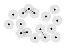
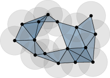
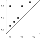
In practice, the underlying manifold is unknown and we are working with a point cloud and a metric such as the Euclidean distance. Persistent homology extends simplicial homology to this setting: instead of approximating by means of a single simplicial complex, which would be an unstable procedure due to the discrete nature of , persistent homology tracks changes in the homology groups over multiple scales of the metric. This is achieved by constructing a special simplicial complex, the Vietoris–Rips complex (Vietoris, 1927). For , the Vietoris–Rips complex of at scale , denoted by , contains all simplices (i.e. subsets) of whose elements satisfy for all , . Given a matrix of pairwise distances of a point cloud , we will use and interchangeably because constructing only requires distances. Vietoris–Rips complexes satisfy a nesting relation, i.e. for , making it possible to track changes in the homology groups as increases (Edelsbrunner et al., 2002). Figure 1 illustrates this process. Since contains a finite number of points, a maximum value exists for which the connectivity stabilises; therefore, calculating is sufficient to obtain topological features at all scales.
We write for the persistent homology calculation of the Vietoris–Rips complex. It results in a tuple of persistence diagrams (st component) and persistence pairings (nd component). The -dimensional persistence diagram (Figure 1(d)) of contains coordinates of the form , where refers to a threshold at which a -dimensional topological feature is created in the Vietoris–Rips complex, and refers to a threshold at which it is destroyed (please refer to Supplementary Section A.1 for a detailed explanation). When , for example, the threshold indicates at which distance two connected components in are merged into one. This calculation is known to be related to spanning trees (Kurlin, 2015) and single-linkage clustering, but the persistence diagrams and the persistence pairings carry more information than either one of these concepts.
The -dimensional persistence pairing contains indices corresponding to simplices that create and destroy the topological feature identified by , respectively. Persistence diagrams are known to be stable with respect to small perturbations in the data set (Cohen-Steiner et al., 2007). Two diagrams and can be compared using the bottleneck distance , where denotes a bijection between the points of the two diagrams, and refers to the norm. We use to refer to the set of persistence diagrams of a point cloud arising from .
3 A Topology-Preserving Autoencoder
We propose a generic framework for constraining autoencoders to preserve topological structures (measured via persistent homology) of the data space in their latent encodings. Figure 2 depicts an overview of our method; the subsequent sections will provide more details about the individual steps.
3.1 Vietoris–Rips Complex Calculation
Given a finite metric space , such as a point cloud, we first calculate the persistent homology of the Vietoris–Rips complex of its distance matrix . It is common practice to use the Euclidean distance for the calculation of , but both the persistent homology calculation and our method are not restricted to any particular distance; previous research (Wagner & Dłotko, 2014) shows that even similarity measures that do not satisfy the properties of a metric can be used successfully with . Subsequently, let so that is the corresponding Vietoris–Rips complex as described in Section 2. Given a maximum dimension111This means that we do not have to consider higher-dimensional topological features, making the calculation more efficient. of , we obtain a set of persistence diagrams , and a set of persistence pairings . The th persistence pairing contains indices of simplices that are pertinent to the creation and destruction of -dimensional topological features. We can consider each pairing to represent edge indices, namely the edges that are deemed to be “topologically relevant” by the computation of persistent homology (see below for more details). This works because the Vietoris–Rips complex is a clique complex, i.e. a simplicial complex that is fully determined by its edges (Zomorodian, 2010).
Selecting indices from pairings
The basic idea of our method involves selecting indices in the persistence pairing and mapping them back to a distance between two vertices. We then adjust this distance to harmonise topological features of the input space and the latent space. For -dimensional topological features, it is sufficient to consider the indices of edges, which are the “destroyer” simplices, in the pairing . Each index corresponds to an edge in the minimum spanning tree of the data set. This calculation is computationally efficient, having a worst-case complexity of , where is the batch size and denotes the extremely slow-growing inverse Ackermann function (Cormen et al., 2009, Chapter 22). For -dimensional features, where edges are paired with triangles, we obtain edge indices by selecting the edge with the maximum weight of the triangle. While this procedure, and thus our method, generalises to higher dimensions, our current implementation supports no higher-dimensional features. Since preliminary experiments showed that using -dimensional topological features merely increases runtime, the subsequent experiments will focus only on -dimensional persistence diagrams. We thus use to denote the 0-dimensional persistence diagram and pairing of , respectively.
3.2 Topological Autoencoder
In the following, we consider a mini-batch of size from the data space as a point cloud. Furthermore, we define an autoencoder as the composition of two functions , where represents the encoder and represents the decoder, denoting latent codes by . During a forward pass of the autoencoder, we compute the persistent homology of the mini-batch in both the data as well as the latent space, yielding two sets of tuples, i.e. and . The values of the persistence diagram can be retrieved by subsetting the distance matrix with the edge indices provided by the persistence pairings; we write to indicate that the diagram, which is a set, contains the same information as the distances we retrieve with the pairing. We treat as a vector in . Informally speaking, the persistent homology calculation can thus be seen as a selection of topologically relevant edges of the Vietoris–Rips complex, followed by the selection of corresponding entries in the distance matrix. By comparing both diagrams, we can construct a topological regularisation term , which we add to the reconstruction loss of an autoencoder, i.e.
| (1) |
where is a parameter to control the strength of the regularisation (see also Supplementary Section A.6).
Next, we discuss how to specify . Since we only select edge indices from and , the calculation represents a selection of topologically relevant distances from the distance matrix. Each persistence diagram entry corresponds to a distance between two data points. Following standard assumptions in persistent homology (Poulenard et al., 2018, Hofer et al., 2019a), we assume that the distances are unique so that each entry in the diagram has an infinitesimal neighbourhood that only contains a single point. In practice, this can always be achieved by performing (symbolic) perturbations of the distances. Given this fixed pairing and a differentiable distance function, the persistence diagram entries are therefore also differentiable with respect to the encoder parameters. Hence, the persistence pairing does not change upon a small perturbation of the underlying distances, thereby guaranteeing the existence of the derivative of our loss function. This, in turn, permits the calculation of gradients for backpropagation.
A straightforward approach to impose the data space topology on the latent space would be to directly calculate a loss based on the selected distances in both spaces. Such an approach will not result in informative gradients for the autoencoder, as it merely compares topological features without matching222We use the term “matching” only to build intuition. Our approach does not calculate a matching in the sense of a bottleneck or Wasserstein distance between persistence diagrams. the edges between and . A cleaner approach would be to enforce similarity on the intersection of the selected edges in both complexes. However, this would initially include very few edges, preventing efficient training and leading to highly biased estimates of the topological alignments between the spaces333When initialising a random latent space , the persistence pairing in the latent space will select random edges, resulting in only expected matched edge (independent of mini-batch size) between the two pairings. Thus, only one edge (referring to one pairwise distance between two latent codes) could be used to update the encoding of these two data points. . To overcome this, we account for the union of all selected edges in and . Our topological loss term decomposes into two components, each handling the “directed” loss occurring as topological features in one of the two spaces remain fixed. Hence, , with
| (2) | |||
| and | |||
| (3) | |||
respectively. The key idea for both terms is to align and preserve topologically relevant distances from both spaces. By taking the union of all selected edges (and the corresponding distances), we obtain an informative loss term that is determined by at least distances. This loss can be seen as a more generic version of the loss introduced by Hofer et al. (2019a), whose formulation does not take the two directed components into account and optimises the destruction values of all persistence tuples with respect to a uniform parameter (their goal is different from ours and does not require a loss term that is capable of harmonising topological features across the two spaces; please refer to Section 4 for a brief discussion). By contrast, our formulation aims to to align the distances between and (which in turn will lead to an alignment of distances between and ). If the two spaces are aligned perfectly, because both pairings and their corresponding distances coincide. The converse implication is not true: if , the persistence pairings and their corresponding persistence diagrams are not necessarily identical. Since we did not observe such behaviour in our experiments, however, we leave a more formal treatment of these situations for future work.
Gradient calculation
Letting refer to the parameters of the encoder and using , we have
| (4) | ||||
| (5) | ||||
| (6) |
where denotes the cardinality of a persistence pairing and refers to the th entry of the vector of paired distances. This derivation works analogously for (with being replaced by ). Furthermore, any derivative of with respect to must vanish because the distances of the input samples do not depend on the encoding by definition. These equations assume infinitesimal perturbations. The persistence diagrams change in a non-differentiable manner during the training phase. However, for any given update step, a diagram is robust to infinitesimal changes of its entries (Cohen-Steiner et al., 2007). As a consequence, our topological loss is differentiable for each update step during training. We make our code publicly available444https://github.com/BorgwardtLab/topological-autoencoders .
3.3 Stability
Despite the aforementioned known stability of persistence diagrams with respect to small perturbations of the underlying space, we still have to analyse our topological approximation on the level of mini-batches. The following theorem guarantees that subsampled persistence diagrams are close to the persistence diagrams of the original point cloud.
Theorem 1.
Let be a point cloud of cardinality and be one subsample of of cardinality , i.e. , sampled without replacement. We can bound the probability of the persistence diagrams of exceeding a threshold in terms of the bottleneck distance as
| (7) |
where refers to the Hausdorff distance between the point cloud and its subsample.
Proof.
See Section A.2 in the supplementary materials. ∎
For , each mini-batch converges to the original point cloud, so we have . Please refer to Section A.3 for an analysis of empirical convergence rates as well as a discussion of a worst-case bound. Given certain independence assumptions, the next theorem approximates the expected value of the Hausdorff distance between the point cloud and a mini-batch. The calculation of an exact representation is beyond the scope of this work.
Theorem 2.
Let be the distance matrix between samples of and , where the rows are sorted such that the first rows correspond to the columns of the subsampled points with diagonal elements . Assume that the entries with are random samples following a distance distribution with . The minimal distances for rows with follow a distribution . Letting with a corresponding distribution , the expected Hausdorff distance between and for is bounded by
| (8) | ||||
| (9) | ||||
| where | ||||
| (10) | ||||
Proof.
See Section A.4 in the supplementary materials. ∎
From Eq. 9, we obtain as , so the expected value converges as the subsample size approaches the total sample size555For , the two integrals switch their order as (for ).. We conclude that our subsampling approach results in point clouds that are suitable proxies for the large-scale topological structures of the point cloud .
4 Related Work
Computational topology and persistent homology (PH) have started gaining traction in several areas of machine learning research. PH is often used as as post hoc method for analysing topological characteristics of data sets. Thus, there are several methods that compare topological features of high-dimensional spaces with different embeddings to assess the fidelity and quality of a specific embedding scheme (Rieck & Leitte, 2017, 2015, Paul & Chalup, 2017, Khrulkov & Oseledets, 2018, Yan et al., 2018). PH can also be used to characterise the training of neural networks (Guss & Salakhutdinov, 2018, Rieck et al., 2019b), as well as their decision boundaries (Ramamurthy et al., 2019). Our method differs from all these publications in that we are able to obtain gradient information to update a model while training. Alternatively, topological features can be integrated into classifiers to improve classification performance. Hofer et al. (2017) propose a neural network layer that learns projections of persistence diagrams, which can subsequently be used as feature descriptors to classify structured data. Moreover, several vectorisation strategies for persistence diagrams exist (Carrière et al., 2015, Adams et al., 2017), making it possible to use them in kernel-based classifiers. These strategies have been subsumed (Carrière et al., 2019) in a novel architecture based on deep sets. The commonality of these approaches is that they treat persistence diagrams as being fixed; while they are capable of learning suitable parameters for classifying them, they cannot adjust input data to better approximate a certain topology.
Such topology-based adjustments have only recently become feasible. Poulenard et al. (2018) demonstrated how to optimise real-valued functions based on their topology. This constitutes the first approach for aligning persistence diagrams by modifying input data; it requires the connectivity of the data to be known, and the optimised functions have to be node-based and scalar-valued. By contrast, our method works directly on distances and sidesteps connectivity calculations via the Vietoris–Rips complex. Chen et al. (2019) use a similar optimisation technique to regularise the decision boundary of a classifier. However, this requires discretising the space, which can be computationally expensive. Hofer et al. (2019a), the closest work to ours, also presents a differentiable loss term. Their formulation enforces a single scale, referred to as , on the latent space. The learned encoding is then applied to a one-class learning task in which a scoring function is calculated based on the pre-defined scale. By contrast, the goal of our loss term is to support the model in learning a latent encoding that best preserves the data space topology in said latent space, which we use for dimensionality reduction. We thus target a different task, and can preserve multiple scales (those selected through the filtration process) that are present in the data domain.
5 Experiments
Our main task is to learn a latent space in an unsupervised manner such that topological features of the data space, measured using persistent homology approximations on every batch, are preserved as much as possible.
5.1 Experimental Setup
Subsequently, we briefly describe our data sets and evaluation metrics. Please refer to the supplementary materials for technical details (calculation, hyperparameters, etc.).
5.1.1 Data Sets
We generate a Spheres data set that consists of ten high-dimensional -spheres living in a -dimensional space that are enclosed by one larger sphere that consists of the same number of points as the total of inner spheres (see Section A.5 for more details). We also use three image data sets (MNIST, Fashion-MNIST, and CIFAR-10), which are particularly amenable to our topology-based analysis because real-world images are known to lie on or near low-dimensional manifolds (Lee et al., 2003, Peyré, 2009).
5.1.2 Baselines & Training Procedure
We compare our approach with several dimensionality reduction techniques, including UMAP (McInnes et al., 2018), t-SNE (van der Maaten & Hinton, 2008), Isomap (Tenenbaum et al., 2000), PCA, as well as standard autoencoders (AE). We apply our proposed topological constraint to this standard autoencoder architecture (TopoAE).
For comparability and interpretability, each method is restricted to two latent dimensions. We split each data set into training and testing (using the predefined split if available; 90% versus 10% otherwise). Additionally, we remove 15% of the training split as a validation data set for tuning the hyperparameters. We normalised our topological loss term by the batch size in order to disentangle from it. All autoencoders employ batch-norm and are optimised using ADAM (Kingma & Ba, 2014). Since t-SNE is not intended to be applied to previously unseen test samples, we evaluate this method only on the train split. In addition, significant computational scaling issues prevent us from running a hyperparameter search for Isomap on real-world data sets, so we only compare this algorithm on the synthetic data set. Please refer to Section A.6 for more details on architectures and hyperparameters.

5.1.3 Evaluation
We evaluate the quality of latent representations in terms of (1) low-dimensional visualisations, (2) dimensionality reduction quality metrics (evaluated between input data and latent codes), and (3) reconstruction errors (Data MSE; evaluated between input and reconstructed data), provided that invertible transformations are available666Invertible transformations are available for PCA and all autoencoder-based methods.. For (2), we consider several measures (please refer to Section A.7 for more details). First, we calculate , the Kullback–Leibler divergence between the density estimates of the input and latent space, based on density estimates (Chazal et al., 2011, 2014b), where denotes the length scale of the Gaussian kernel, which is varied to account for multiple data scales. We chose minimising as our hyperparameter search objective. Furthermore, we calculate common non-linear dimensionality reduction (NLDR) quality metrics, which use the pairwise distance matrices of the input and the latent space (as indicated by the “” in the abbreviations), namely (1) the root mean square error (-RMSE), which—despite its name—is not related to the reconstruction error of the autoencoder but merely measures to what extent the two distributions of distances coincide, (2) the mean relative rank error (-MRRE), (3) the continuity (-Cont), and (4) the trustworthiness (-Trust) . The reported measures are computed on the test splits (except for t-SNE where no transformation between splits is available, so we report the measures on a random subsample of the train split, preserving the cardinality of the test split).
Fashion-MNIST
MNIST
CIFAR-10
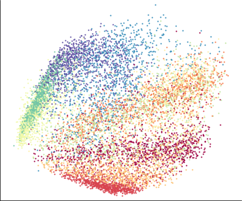
PCA
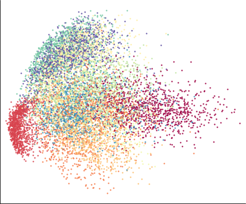
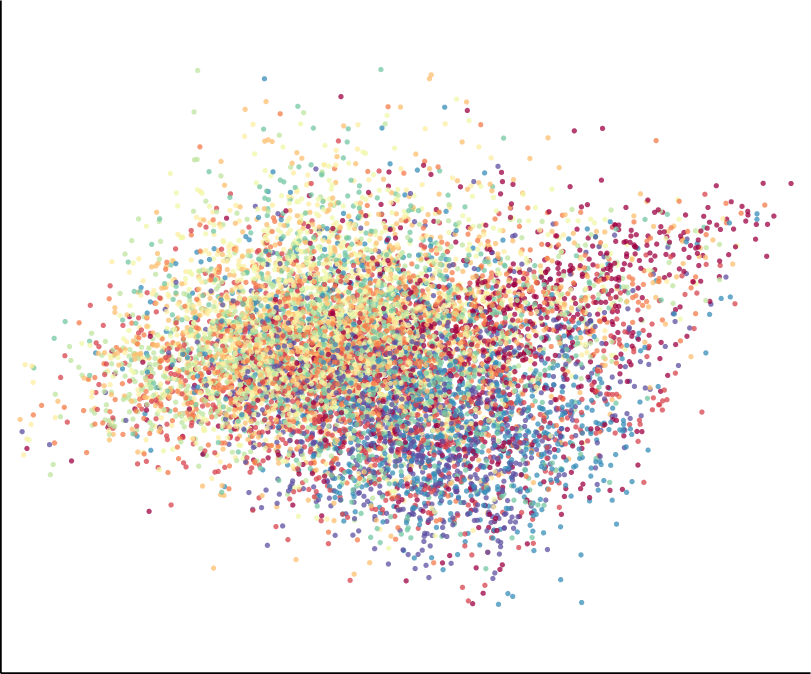
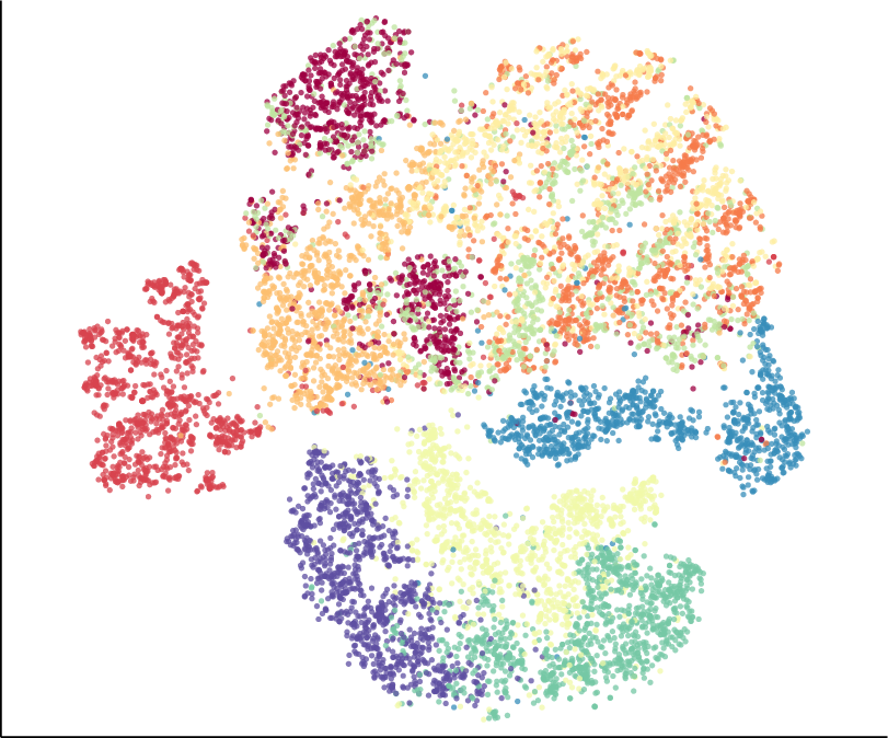
t-SNE
UMAP
AE
TopoAE
5.2 Results
Next to a quantitative evaluation in terms of various quality metrics, we also discuss qualitative results in terms of visualisations, which are interpretable in case the ground truth manifold is known.
| Data set | Method | -MRRE | -Cont | -Trust | -RMSE | Data MSE | |||
|---|---|---|---|---|---|---|---|---|---|
| Spheres | Isomap | 0.181 | 0.420 | 0.00881 | 0.246 | 0.790 | 0.676 | 10.4 | – |
| PCA | 0.332 | 0.651 | 0.01530 | 0.294 | 0.747 | 0.626 | 11.8 | 0.9610 | |
| TSNE | 0.152 | 0.527 | 0.01271 | 0.217 | 0.773 | 0.679 | 8.1 | – | |
| UMAP | 0.157 | 0.613 | 0.01658 | 0.250 | 0.752 | 0.635 | 9.3 | – | |
| AE | 0.566 | 0.746 | 0.01664 | 0.349 | 0.607 | 0.588 | 13.3 | 0.8155 | |
| TopoAE | 0.085 | 0.326 | 0.00694 | 0.272 | 0.822 | 0.658 | 13.5 | 0.8681 | |
| F-MNIST | PCA | 0.356 | 0.052 | 0.00069 | 0.057 | 0.968 | 0.917 | 9.1 | 0.1844 |
| TSNE | 0.405 | 0.071 | 0.00198 | 0.020 | 0.967 | 0.974 | 41.3 | – | |
| UMAP | 0.424 | 0.065 | 0.00163 | 0.029 | 0.981 | 0.959 | 13.7 | – | |
| AE | 0.478 | 0.068 | 0.00125 | 0.026 | 0.968 | 0.974 | 20.7 | 0.1020 | |
| TopoAE | 0.392 | 0.054 | 0.00100 | 0.032 | 0.980 | 0.956 | 20.5 | 0.1207 | |
| MNIST | PCA | 0.389 | 0.163 | 0.00160 | 0.166 | 0.901 | 0.745 | 13.2 | 0.2227 |
| TSNE | 0.277 | 0.133 | 0.00214 | 0.040 | 0.921 | 0.946 | 22.9 | – | |
| UMAP | 0.321 | 0.146 | 0.00234 | 0.051 | 0.940 | 0.938 | 14.6 | – | |
| AE | 0.620 | 0.155 | 0.00156 | 0.058 | 0.913 | 0.937 | 18.2 | 0.1373 | |
| TopoAE | 0.341 | 0.110 | 0.00114 | 0.056 | 0.932 | 0.928 | 19.6 | 0.1388 | |
| CIFAR | PCA | 0.591 | 0.020 | 0.00023 | 0.119 | 0.931 | 0.821 | 17.7 | 0.1482 |
| TSNE | 0.627 | 0.030 | 0.00073 | 0.103 | 0.903 | 0.863 | 25.6 | – | |
| UMAP | 0.617 | 0.026 | 0.00050 | 0.127 | 0.920 | 0.817 | 33.6 | – | |
| AE | 0.668 | 0.035 | 0.00062 | 0.132 | 0.851 | 0.864 | 36.3 | 0.1403 | |
| TopoAE | 0.556 | 0.019 | 0.00031 | 0.108 | 0.927 | 0.845 | 37.9 | 0.1398 |
5.2.1 Quantitative Results
Table 1 reports the quantitative results. Overall, we observe that our method is capable of preserving the data density over multiple length scales (as measured by ). Furthermore, we find that TopoAE displays competitive continuity values (-Cont) and reconstruction errors (Data MSE). The latter is particularly relevant as it demonstrates that imposing our topological constraints does not result in large impairments when reconstructing the input space.
The remaining classical measures favour the baselines (foremost the train (!) performance of t-SNE). However, we will subsequently see by inspecting the latent spaces that those classic measures fail to detect the relevant structural information, as exemplified with known ground truth manifolds, such as the Spheres data set.
5.2.2 Visualisation of Latent Spaces
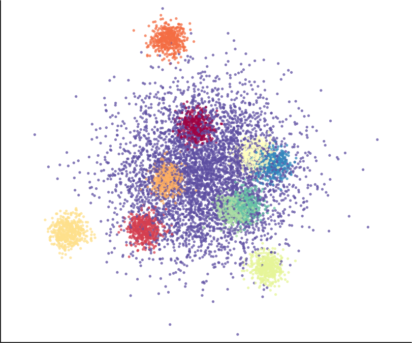
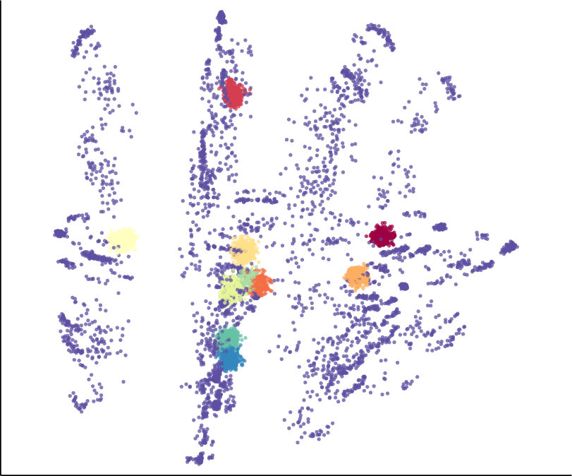
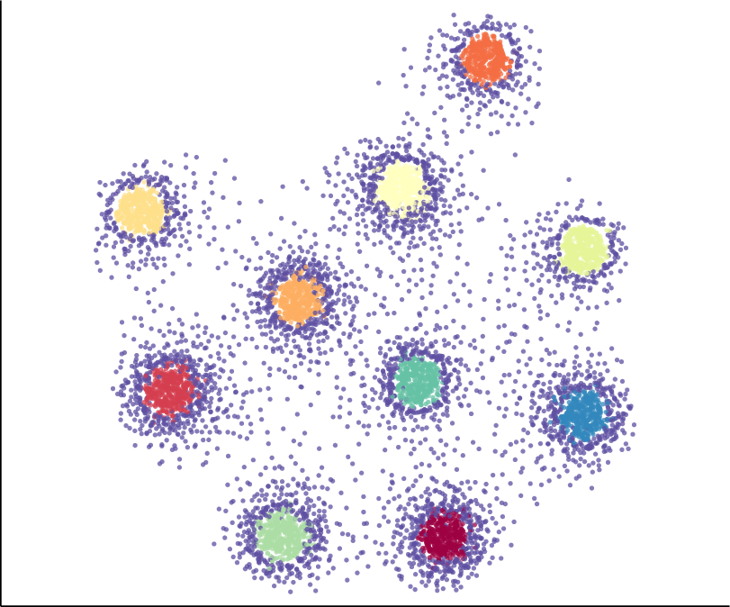
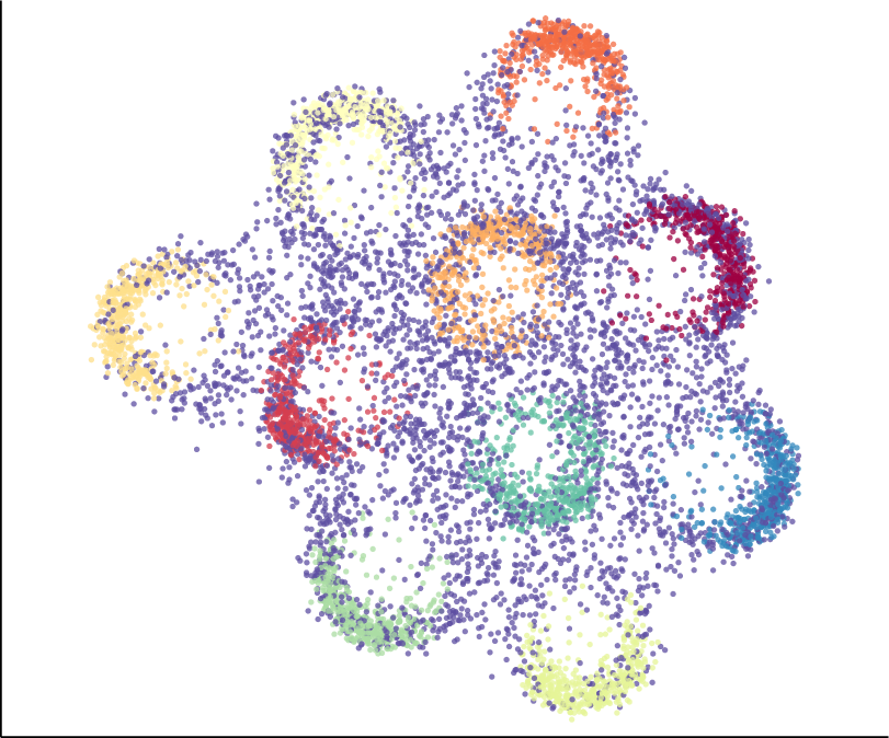
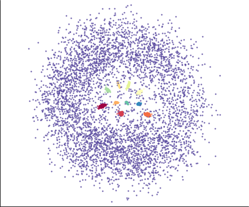
For the Spheres data set (Figure 3), we observe that only our method is capable of assessing the nesting relationship of the high-dimensional spheres correctly. By contrast, t-SNE “cuts open” the enclosing sphere, distributing most of its points around the remaining spheres. We see that the -divergence confirms the visual assessment that only our proposed method preserves the relevant structure of this data set. Several classical evaluation measures, however, favour t-SNE, even though this method fails to capture the global structure and nesting relationship of the enclosing sphere manifold accounting for half of the data set.
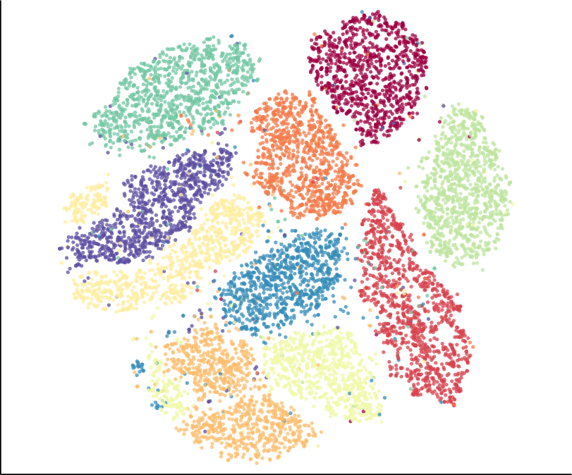
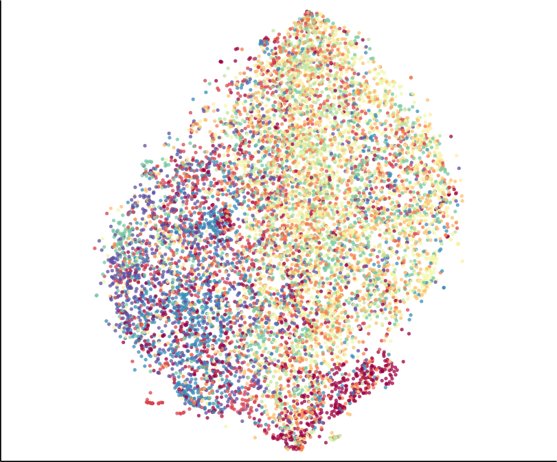
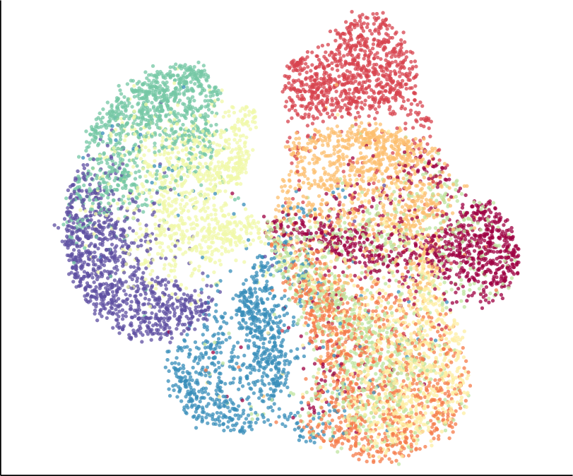
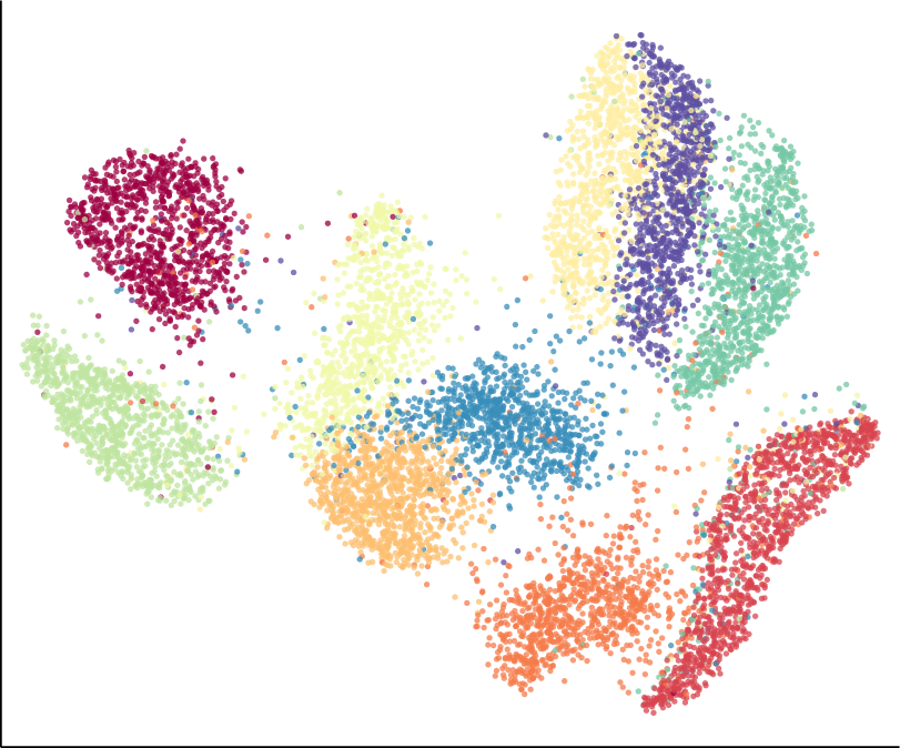
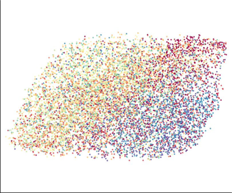
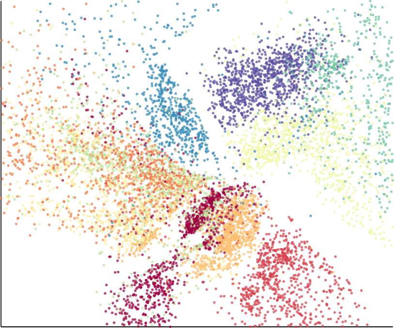
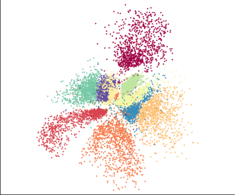
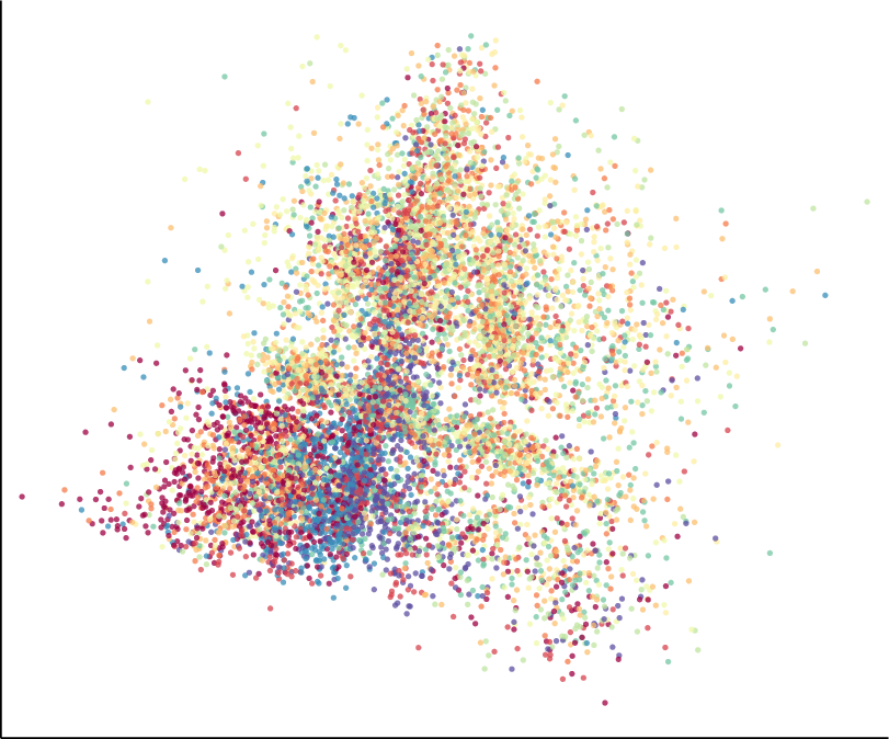
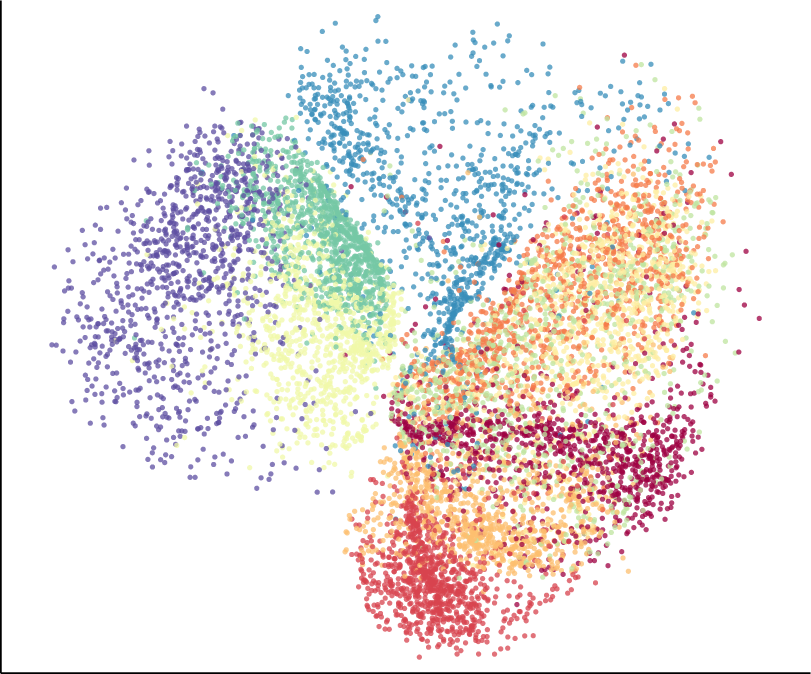
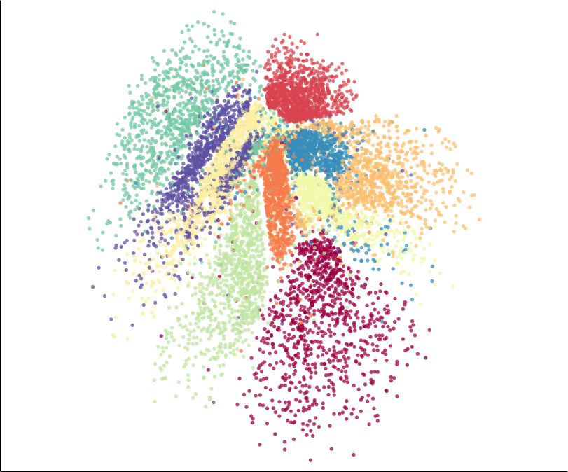
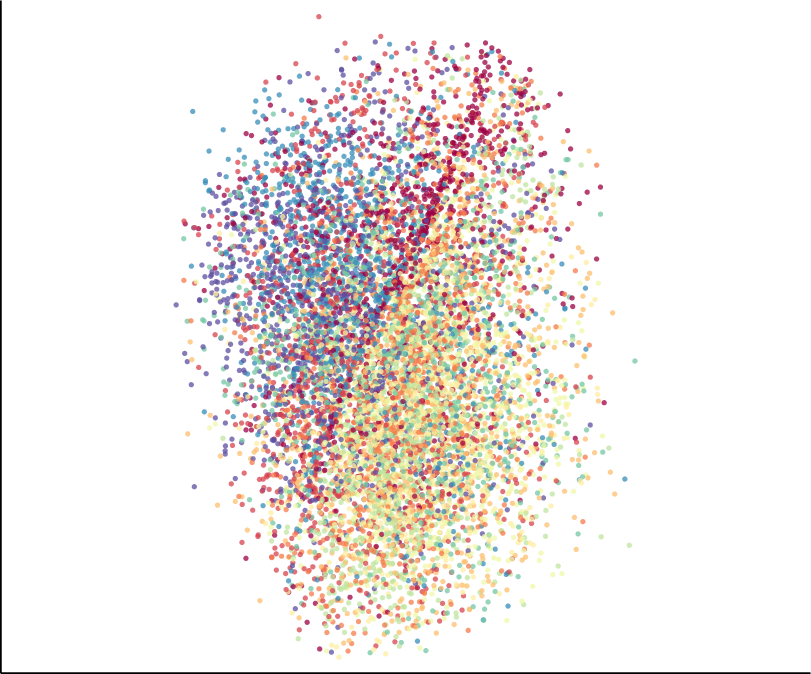
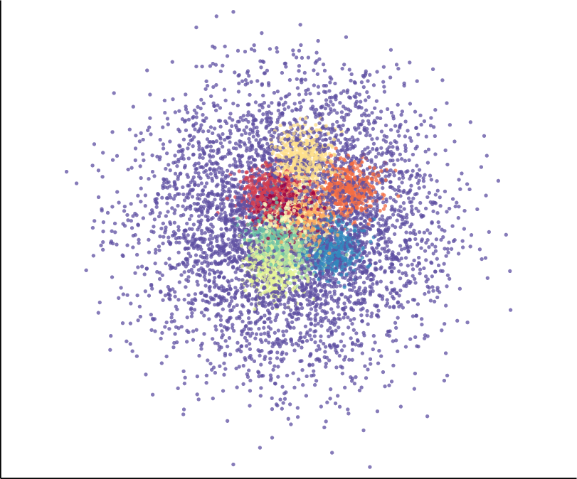
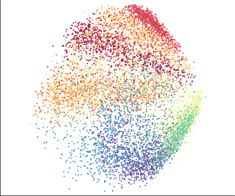
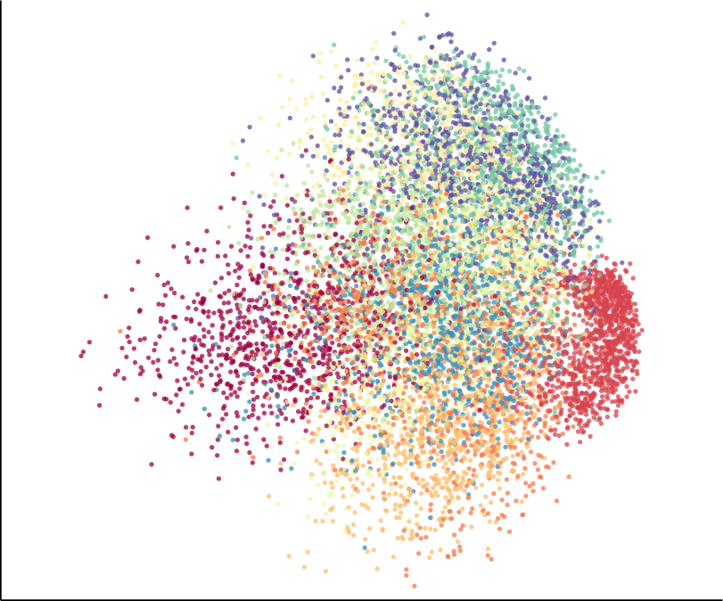
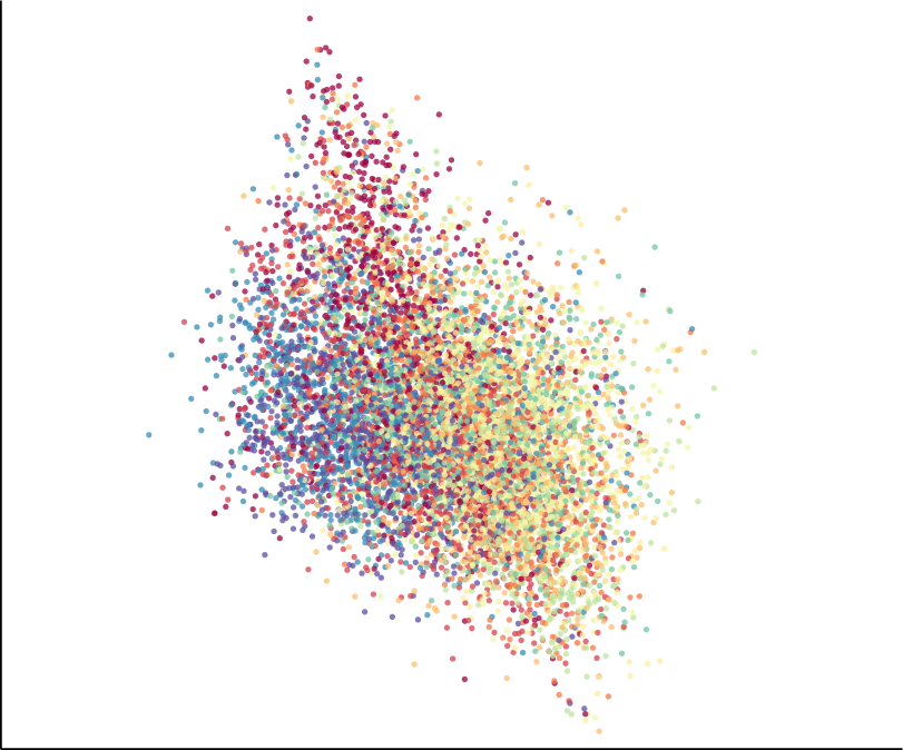
On Fashion-MNIST (Figure 4, leftmost column), we see that, as opposed to AE, which is purely driven by the reconstruction error, our method has the additional objective of preserving structure. Here, the constraint helps the regularised autoencoder to “organise” the latent space, resulting in a comparable pattern as in UMAP, which is also topologically motivated (McInnes et al., 2018). Furthermore, we observe that t-SNE tends to fragment certain classes (dark orange, red) into multiple distinct subgroups. This likely does not reflect the underlying manifold structure, but constitutes an artefact frequently observed with this method. For MNIST, the latent embeddings (Figure 4, middle column) demonstrate that the non-linear competitors—mostly by pulling apart distinct classes—lose some of the relationship information between clusters when comparing against our proposed method or PCA. Finally, we observe that CIFAR-10 (Figure 4, rightmost column), is challenging to embed in two latent dimensions in a purely unsupervised manner. Interestingly, our method (consistently, i.e. over all runs) was able to identify a linear substructure that separates the latent space in two additional groups of classes.
6 Discussion and Conclusion
We presented topological autoencoders, a novel method for preserving topological information, measured in terms of persistent homology, of the input space when learning latent representations with deep neural networks. Under weak theoretical assumptions, we showed how our persistent homology calculations can be combined with backpropagation; moreover, we proved that approximating persistent homology on the level of mini-batches is theoretically justified.
In our experiments, we observed that our method is uniquely able to capture spatial relationships between nested high-dimensional spheres. This is relevant, as the ability to cope with several manifolds in the domain of manifold learning still remains a challenging task. On real-world data sets, we observed that our topological loss leads to competitive performance in terms of numerous quality metrics (such as a density preservation metric), while not adversely affecting the reconstruction error. In both synthetic and real-world data sets, we obtain interesting and interpretable representations, as our method does not merely pull apart different classes, but tries to spatially arrange them meaningfully. Thus, we do not observe mere distinct “clouds”, but rather entangled structures, which we consider to constitute a more meaningful representation of the underlying manifolds (an auxiliary analysis in Supplementary Section A.10 confirms that our method influences topological features, measured using PH, in a beneficial manner).
Future work
Our topological loss formulation is highly generalisable; it only requires the existence of a distance matrix between individual samples (either globally, or on the level of batches). As a consequence, our topological loss term can be directly integrated into a variety of different architectures and is not limited to standard autoencoders. For instance, we can also apply our constraint to variational setups (see Figure A.3 for a sketch) or create a topology-aware variant of principal component analysis (dubbed “TopoPCA”; see Table A.2 for more details, as well as Figures A.6, A.7, and A.8 for the corresponding latent space representations). Employing our loss term to more involved architectures will be an exciting route for future work. One issue with the calculation is that, given the computational complexity of calculating , for higher-dimensional features, we would scale progressively worse with increasing batch size. However, in our low-dimensional setup, we observed that runtime tends to grow with decreasing batch size, i.e. the mini-batch speed-up still dominates runtime (for more details concerning the effect of batch sizes, see Supplementary Section A.8). In future work, scaling to higher dimensions could be mitigated by approximating the calculation of persistent homology (Choudhary et al., 2018, Kerber & Sharathkumar, 2013, Sheehy, 2013) or by exploiting recent advances in parallelising it (Bauer et al., 2014, Lewis & Morozov, 2015). Another interesting extension would be to tackle classification scenarios with topology-preserving loss terms. This might prove challenging, however, because the goal in classification is to increase class separability, which might be achieved by removing topological structures. This goal is therefore at odds with our loss term that tries preserving those structures. We think that such an extension might require restricting the method to a subset of scales (namely those that do not impede class separability) to be preserved in the data.
Acknowledgements
The authors wish to thank Christian Bock for fruitful discussions and valuable feedback.
This project was supported by the grant #2017-110 of the Strategic Focal Area “Personalized Health and Related Technologies (PHRT)” of the ETH Domain for the SPHN/PHRT Driver Project “Personalized Swiss Sepsis Study” and the SNSF Starting Grant “Significant Pattern Mining” (K.B., grant no. 155913). Moreover, this work was funded in part by the Alfried Krupp Prize for Young University Teachers of the Alfried Krupp von Bohlen und Halbach-Stiftung (K.B.).
References
- Adams et al. (2017) Adams, H., Emerson, T., Kirby, M., Neville, R., Peterson, C., Shipman, P., Chepushtanova, S., Hanson, E., Motta, F., and Ziegelmeier, L. Persistence images: A stable vector representation of persistent homology. Journal of Machine Learning Research, 18(1):218–252, 2017.
- Barannikov (1994) Barannikov, S. A. The framed Morse complex and its invariants. Advances in Soviet Mathematics, 21:93–115, 1994.
- Bauer et al. (2014) Bauer, U., Kerber, M., and Reininghaus, J. Distributed computation of persistent homology. In McGeoch, C. C. and Meyer, U. (eds.), Proceedings of the Sixteenth Workshop on Algorithm Engineering and Experiments (ALENEX), pp. 31–38. Society for Industrial and Applied Mathematics, 2014.
- Bibal & Frénay (2019) Bibal, A. and Frénay, B. Measuring quality and interpretability of dimensionality reduction visualizations. Safe Machine Learning Workshop at ICLR, 2019.
- Burago et al. (2001) Burago, D., Burago, Y., and Ivanov, S. A course in metric geometry, volume 33 of Graduate Studies in Mathematics. American Mathematical Society, 2001.
- Carrière et al. (2015) Carrière, M., Oudot, S. Y., and Ovsjanikov, M. Stable topological signatures for points on 3D shapes. In Proceedings of the Eurographics Symposium on Geometry Processing (SGP), pp. 1–12, Aire-la-Ville, Switzerland, 2015. Eurographics Association.
- Carrière et al. (2019) Carrière, M., Chazal, F., Ike, Y., Lacombe, T., Royer, M., and Umeda, Y. PersLay: A neural network layer for persistence diagrams and new graph topological signatures. arXiv e-prints, art. arXiv:1904.09378, 2019.
- Chazal et al. (2009) Chazal, F., Cohen-Steiner, D., Guibas, L. J., Mémoli, F., and Oudot, S. Y. Gromov–Hausdorff stable signatures for shapes using persistence. Computer Graphics Forum, 28(5):1393–1403, 2009.
- Chazal et al. (2011) Chazal, F., Cohen-Steiner, D., and Mérigot, Q. Geometric inference for probability measures. Foundations of Computational Mathematics, 11(6):733–751, 2011.
- Chazal et al. (2014a) Chazal, F., de Silva, V., and Oudot, S. Y. Persistence stability for geometric complexes. Geometriæ Dedicata, 173(1):193–214, 2014a.
- Chazal et al. (2014b) Chazal, F., Fasy, B. T., Lecci, F., Michel, B., Rinaldo, A., and Wasserman, L. Robust topological inference: Distance to a measure and kernel distance. arXiv e-prints, art. arXiv:1412.7197, 2014b.
- Chazal et al. (2015a) Chazal, F., Fasy, B., Lecci, F., Michel, B., Rinaldo, A., and Wasserman, L. Subsampling methods for persistent homology. In Bach, F. and Blei, D. (eds.), Proceedings of the 32nd International Conference on Machine Learning (ICML), volume 37 of Proceedings of Machine Learning Research, pp. 2143–2151. PMLR, 2015a.
- Chazal et al. (2015b) Chazal, F., Glisse, M., Labruère, C., and Michel, B. Convergence rates for persistence diagram estimation in topological data analysis. Journal of Machine Learning Research, 16:3603–3635, 2015b.
- Chen et al. (2019) Chen, C., Ni, X., Bai, Q., and Wang, Y. A topological regularizer for classifiers via persistent homology. In Chaudhuri, K. and Sugiyama, M. (eds.), Proceedings of Machine Learning Research, volume 89 of Proceedings of Machine Learning Research, pp. 2573–2582. PMLR, 2019.
- Choudhary et al. (2018) Choudhary, A., Kerber, M., and Raghvendra, S. Improved topological approximations by digitization. arXiv e-prints, art. arXiv:1812.04966, 2018.
- Cohen-Steiner et al. (2007) Cohen-Steiner, D., Edelsbrunner, H., and Harer, J. Stability of persistence diagrams. Discrete & Computational Geometry, 37(1):103–120, 2007.
- Cormen et al. (2009) Cormen, T. H., Leiserson, C. E., Rivest, R. L., and Stein, C. Introduction to algorithms. MIT Press, Cambridge, MA, USA, 3rd edition, 2009.
- Edelsbrunner & Harer (2008) Edelsbrunner, H. and Harer, J. Persistent homology—a survey. In Goodman, J. E., Pach, J., and Pollack, R. (eds.), Surveys on discrete and computational geometry: Twenty years later, number 453 in Contemporary Mathematics, pp. 257–282. American Mathematical Society, Providence, RI, USA, 2008.
- Edelsbrunner et al. (2002) Edelsbrunner, H., Letscher, D., and Zomorodian, A. J. Topological persistence and simplification. Discrete & Computational Geometry, 28(4):511–533, 2002.
- Gracia et al. (2014) Gracia, A., González, S., Robles, V., and Menasalvas, E. A methodology to compare dimensionality reduction algorithms in terms of loss of quality. Information Sciences, 270:1–27, 2014.
- Guss & Salakhutdinov (2018) Guss, W. H. and Salakhutdinov, R. On characterizing the capacity of neural networks using algebraic topology. arXiv e-prints, art. arXiv:1802.04443, 2018.
- Hinton & Salakhutdinov (2006) Hinton, G. E. and Salakhutdinov, R. R. Reducing the dimensionality of data with neural networks. Science, 313(5786):504–507, 2006.
- Hofer et al. (2017) Hofer, C., Kwitt, R., Niethammer, M., and Uhl, A. Deep learning with topological signatures. In Guyon, I., Luxburg, U. V., Bengio, S., Wallach, H., Fergus, R., Vishwanathan, S., and Garnett, R. (eds.), Advances in Neural Information Processing Systems 30, pp. 1633–1643. Curran Associates, Inc., 2017.
- Hofer et al. (2019a) Hofer, C., Kwitt, R., Niethammer, M., and Dixit, M. Connectivity-optimized representation learning via persistent homology. In Chaudhuri, K. and Salakhutdinov, R. (eds.), Proceedings of the 36th International Conference on Machine Learning, volume 97 of Proceedings of Machine Learning Research, pp. 2751–2760. PMLR, 2019a.
- Hofer et al. (2019b) Hofer, C. D., Graf, F., Rieck, B., Niethammer, M., and Kwitt, R. Graph filtration learning. arXiv e-prints, art. arXiv:1905.10996, 2019b.
- Kerber & Sharathkumar (2013) Kerber, M. and Sharathkumar, R. Approximate Čech complexes in low and high dimensions. arXiv e-prints, art. arXiv:1307.3272, 2013.
- Khrulkov & Oseledets (2018) Khrulkov, V. and Oseledets, I. Geometry score: A method for comparing generative adversarial networks. In Dy, J. and Krause, A. (eds.), Proceedings of the 35th International Conference on Machine Learning, volume 80 of Proceedings of Machine Learning Research, pp. 2621–2629. PMLR, 2018.
- Kingma & Ba (2014) Kingma, D. P. and Ba, J. Adam: A method for stochastic optimization. arXiv e-prints, art. arXiv:1412.6980, 2014.
- Kurlin (2015) Kurlin, V. A one-dimensional homologically persistent skeleton of an unstructured point cloud in any metric space. Computer Graphics Forum, 34(5):253–262, 2015.
- Lee et al. (2003) Lee, A. B., Pedersen, K. S., and Mumford, D. The nonlinear statistics of high-contrast patches in natural images. International Journal of Computer Vision, 54(1–3):83–103, 2003.
- Lee & Verleysen (2009) Lee, J. A. and Verleysen, M. Quality assessment of dimensionality reduction: Rank-based criteria. Neurocomputing, 72(7):1431–1443, 2009.
- Lewis & Morozov (2015) Lewis, R. and Morozov, D. Parallel computation of persistent homology using the blowup complex. In Proceedings of the 27th ACM Symposium on Parallelism in Algorithms and Architectures (SPAA), pp. 323–331. ACM, 2015.
- McInnes et al. (2018) McInnes, L., Healy, J., and Melville, J. UMAP: Uniform manifold approximation and projection for dimension reduction. arXiv e-prints, art. arXiv:1802.03426, 2018.
- Mémoli & Sapiro (2004) Mémoli, F. and Sapiro, G. Comparing point clouds. In Proceedings of the Eurographics/ACM SIGGRAPH Symposium on Geometry Processing (SGP), pp. 32–40, New York, NY, USA, 2004. Association for Computing Machinery.
- Paul & Chalup (2017) Paul, R. and Chalup, S. K. A study on validating non-linear dimensionality reduction using persistent homology. Pattern Recognition Letters, 100:160–166, 2017.
- Peyré (2009) Peyré, G. Manifold models for signals and images. Computer Vision and Image Understanding, 113(2):249–260, 2009.
- Poulenard et al. (2018) Poulenard, A., Skraba, P., and Ovsjanikov, M. Topological function optimization for continuous shape matching. Computer Graphics Forum, 37(5):13–25, 2018.
- Ramamurthy et al. (2019) Ramamurthy, K. N., Varshney, K., and Mody, K. Topological data analysis of decision boundaries with application to model selection. In Chaudhuri, K. and Salakhutdinov, R. (eds.), Proceedings of the 36th International Conference on Machine Learning, volume 97 of Proceedings of Machine Learning Research, pp. 5351–5360. PMLR, 2019.
- Reininghaus et al. (2015) Reininghaus, J., Huber, S., Bauer, U., and Kwitt, R. A stable multi-scale kernel for topological machine learning. In Proceedings of the IEEE Conference on Computer Vision and Pattern Recognition, pp. 4741–4748, 2015.
- Rieck & Leitte (2015) Rieck, B. and Leitte, H. Persistent homology for the evaluation of dimensionality reduction schemes. Computer Graphics Forum, 34(3):431–440, 2015.
- Rieck & Leitte (2017) Rieck, B. and Leitte, H. Agreement analysis of quality measures for dimensionality reduction. In Carr, H., Garth, C., and Weinkauf, T. (eds.), Topological Methods in Data Analysis and Visualization IV. Springer, Cham, Switzerland, 2017.
- Rieck et al. (2019a) Rieck, B., Bock, C., and Borgwardt, K. A persistent Weisfeiler–Lehman procedure for graph classification. In Chaudhuri, K. and Salakhutdinov, R. (eds.), Proceedings of the 36th International Conference on Machine Learning, volume 97 of Proceedings of Machine Learning Research, pp. 5448–5458. PMLR, 2019a.
- Rieck et al. (2019b) Rieck, B., Togninalli, M., Bock, C., Moor, M., Horn, M., Gumbsch, T., and Borgwardt, K. Neural persistence: a complexity measure for deep neural networks using algebraic topology. In International Conference on Learning Representations (ICLR), 2019b.
- scikit-optimize contributers (2018) scikit-optimize contributers, T. scikit-optimize/scikit-optimize: v0.5.2, March 2018.
- Sheehy (2013) Sheehy, D. R. Linear-size approximations to the Vietoris–Rips filtration. Discrete & Computational Geometry, 49(4):778–796, 2013.
- Tenenbaum et al. (2000) Tenenbaum, J. B., De Silva, V., and Langford, J. C. A global geometric framework for nonlinear dimensionality reduction. Science, 290(5500):2319–2323, 2000.
- van der Maaten & Hinton (2008) van der Maaten, L. J. and Hinton, G. Visualizing data using t-SNE. Journal of Machine Learning Research, 9:2579–2605, 2008.
- van der Maaten et al. (2009) van der Maaten, L. J., Postma, E. O., and van den Herik, H. J. Dimensionality reduction: A comparative review. Technical Report 2009-005, Tilburg University, 2009.
- Venna & Kaski (2006) Venna, J. and Kaski, S. Visualizing gene interaction graphs with local multidimensional scaling. In Proceedings of the 14th European Symposium on Artificial Neural Networks, pp. 557–562. d-side publishing, 2006.
- Vietoris (1927) Vietoris, L. Über den höheren Zusammenhang kompakter Räume und eine Klasse von zusammenhangstreuen Abbildungen. Mathematische Annalen, 97(1):454–472, 1927.
- Wagner & Dłotko (2014) Wagner, H. and Dłotko, P. Towards topological analysis of high-dimensional feature spaces. Computer Vision and Image Understanding, 121:21–26, 2014.
- Yan et al. (2018) Yan, L., Zhao, Y., Rosen, P., Scheidegger, C., and Wang, B. Homology-preserving dimensionality reduction via manifold landmarking and tearing. arXiv e-prints, art. arXiv:1806.08460, 2018.
- Zomorodian (2010) Zomorodian, A. J. Fast construction of the Vietoris–Rips complex. Computers & Graphics, 34(3):263–271, 2010.
Appendix A Appendix
A.1 Persistent Homology Calculation Details
This section provides more details about the persistent homology calculation; it is more geared towards an expert reader and aims for a concise description of all required concepts.
Simplicial homology
To understand persistent homology, we first have to understand simplicial homology. Given a simplicial complex , i.e. a high-dimensional generalisation of a graph, let denote the vector space generated over whose elements are the -simplices in 777It is also possible to describe this calculation with coefficients in other fields, but the case of is advantageous because it simplifies the implementation of all operations. . For , let be the boundary homomorphism defined by
| (11) |
for a single simplex and linearly extended to . The th homology group of is defined as the quotient group . The rank of the th homology group is known as the th Betti number , i.e. . The sequence of Betti numbers of a -dimensional simplicial complex is commonly used to distinguish between different manifolds. For example, a -sphere in 3 has Betti numbers , while a -torus in 3 has Betti numbers . Betti numbers are of limited use for analysing real-world data sets, however, because their representation is too coarse and easily affected by small changes in the underlying simplicial complex. In an idealised, platonic setting, this does not pose a problem, because one assumes that the triangulation of a manifold is known a priori; for real-world data sets, however, we are typically dealing with point clouds and have no knowledge of the underlying manifold, making the calculation of the “proper” simplicial complex nigh impossible. These disadvantages prompted the development of persistent homology.
Persistent homology
Let be a nested sequence of simplicial complexes, called filtration. Filtrations can be defined based on different functions; the Vietoris–Rips filtration that we discuss in the paper, for example, is defined by a distance function, such as the Euclidean distance between points of a point cloud. Notice that we may still calculate the simplicial homology of each in the filtration. The filtration provides more information, though: the family of boundary operators , together with the inclusion homomorphism, induces a homomorphism between corresponding homology groups of the filtration, i.e. . This homomorphism yields a sequence of homology groups
for every dimension . Given indices , the th persistent homology group is defined as
| (12) |
It can be seen as the homology group that contains all homology classes created in that are still present (“active”) in . We define the th persistent Betti number to be the rank of this group, i.e. , which generalises the previous definition for simplicial homology. Persistent homology results in a sequence of Betti numbers—instead of a single number—that permits a fine-grained description of topological activity. This activity is typically summarised in a persistence diagram, thus replacing the indices with real numbers based on the function that was used to calculate the filtration.
Persistence diagrams
A filtration often has associated values (or weights) , such as the pairwise distances in a point cloud. These values permit the calculation of topological feature descriptors known as persistence diagrams: for each dimension and each pair , one stores a pair with multiplicity
| (13) |
in a multiset (typically, for many pairs). The pair represents a topological feature that was created at a certain threshold , and destroyed at another threshold . In the case of the Vietoris–Rips filtration and connected components, we have because all connected components are present at the beginning of the filtration by definition. Similarly, will correspond to an edge used in the minimum spanning tree of the data set. In general, the resulting set of points is called the th persistence diagram . Given a point , the quantity is referred to as its persistence.
A.2 Proof of Theorem 1
Theorem 1.
Let be a point cloud of cardinality and be one subsample of of cardinality , i.e. , sampled without replacement. We can bound the probability of exceeding a threshold in terms of the bottleneck distance as
| (14) |
where refers to the Hausdorff distance between the point cloud and its subsample, i.e.
| (15) |
for a baseline distance such as the Euclidean distance.
Proof.
The stability of persistent homology calculations was proved by Chazal et al. (2014a) for finite metric spaces. More precisely, given two metric spaces and , we have
| (16) |
where refers to the Gromov–Hausdorff distance (Burago et al., 2001, p. 254) of the two spaces. It is defined as the infimum Hausdorff distance over all isometric embeddings of and . This distance can be employed for shape comparison (Chazal et al., 2009, Mémoli & Sapiro, 2004), but is hard to compute. In our case, with and , we consider both spaces to have the same metric (for , we take the canonical restriction of the metric from to the subspace ). By definition of the Gromov–Hausdorff distance, we thus have , so Eq. 15 leads to
| (17) |
from which the original claim from Eq. 14 follows by taking probabilities on both sides. ∎
A.3 Empirical Convergence Rates of
Figure A.1 depicts the mean of the convergence rate (mean) of the Hausdorff distance for a subsample of size of points in a -dimensional space, following a standard normal distribution. We can see that the convergence rate is roughly similar, but shown on different absolute levels that depend on the ambient dimension. While bounding the convergence rate of this expression is feasible (Chazal et al., 2015a, b), it requires more involved assumptions on the measures from which and are sampled. Additionally, we can give a simple bound using the diameter . We have because the supremum is guaranteed to be an upper bound for the Hausdorff distance. This worst-case bound does not account for the sample size (or mini-batch size) , though (see Theorem 2 for an expression that takes into account).
A.4 Proof of Theorem 2
Prior to the proof we state two observations that arise from our special setting of dealing with finite point clouds.
Observation 1.
Since , we have . Hence, the Hausdorff distance simplifies to:
| (18) |
In other words, we only have to consider a “one-sided” expression of the distance because the distance from the subsample to the original point cloud is always zero.
Observation 2.
Since our point clouds of interest are finite sets, the suprema and infima of the Hausdorff distance coincide with the maxima and minima, which we will subsequently use for easier readability.
Hence, the computation of can be divided into three steps.
-
1.
Using the baseline distance , we compute a distance matrix between all points in and .
-
2.
For each of the points in , we compute the minimal distance to the samples of by extracting the minimal distance per row of and gather all minimal distances in .
-
3.
Finally, we return the maximal entry of as .
In the subsequent proof, we require an independence assumption of the samples.
Proof.
Using Observations 1 and 2 we obtain a simplified expression for the Hausdorff distance, i.e.
| (19) |
The minimal distances of the first rows of are trivially . Hence, the outer maximum is determined by the remaining row minima { } with . Those minima follow the distribution with
| (20) | ||||
| (21) | ||||
| (22) | ||||
| (23) | ||||
| (24) |
Next, we consider . To evaluate the density of , we first need to derive its distribution :
| (25) | ||||
| (26) |
Next, we approximate by by imposing i.i.d sampling of the minimal distances from . This is an approximation because in practice, the rows to are not stochastically independent because of the triangular inequality that holds for metrics. However, assuming i.i.d., we arrive at
| (27) |
Since has positive support its expectation can then be evaluated as:
| (28) | ||||
| (29) |
The independence assumption leading to results in overestimating the variance of the drawn minima . Thus, the expected maximum of those minima, , is overestimating the actual expectation of the maximum , which is why Eq. 28 constitutes an upper bound of , and equivalently, an upper bound of . ∎
A.5 Synthetic Data Set
Spheres consists of eleven high-dimensional -spheres living in dimensional space. Ten spheres of radius are each shifted in a random direction (by adding the same Gaussian noise vector per sphere). To this end, we draw ten -dimensional Gaussian vectors following for . Crucially, to add interesting topological information to the data set, the ten spheres are enclosed by an additional larger sphere of radius . The spheres were generated using the library scikit-tda.
A.6 Architectures and Hyperparameter Tuning
Architectures for synthetic data set
For the synthetically generated data set, we use a simple multilayer perceptron architecture consisting of two hidden layer with neurons each both encoder and decoder and a bottleneck of two neurons such that the sequence of hidden-layer neurons is . ReLU non-linearities and batch normalization were applied between the layers excluding the output layer and the bottleneck layer. The networks were fit using mean squared error loss.
Architectures for real world data sets
For the MNIST, Fashion-MNIST, and CIFAR-10 data sets, we use an architecture inspired by DeepAE (Hinton & Salakhutdinov, 2006). This architecture is composed of 3 layers of hidden neurons of decreasing size () for the encoder part, a bottleneck of two neurons, and a sequence of three layers of hidden neurons in decreasing size () for the decoder. In contrast to the originally proposed architecture, we applied ReLU non-linearities and batch normalization between the layers as we observed faster and more stable training. For the non-linearities of the final layer, we applied the non-linearity, such that the image of the activation matches the range of input images scaled between and . Also here, we applied mean squared error loss.
All neural network architectures were fit using Adam and weight-decay of .
Hyperparameter tuning
For hyperparameter tuning we apply random sampling of hyperparameters using the scikit-optimize library (scikit-optimize contributers, 2018) with 20 calls per method on all data sets. We select the best model parameters in terms of on the validation split and evaluate and report it on the test split. To estimate performance means and standard deviations, we repeated the evaluation on an independent test split 5 times by using the best parameters (as identified in the hyperparameter search on the validation split) and refitting the models by resampling the train-validation split.
Neural networks
For the neural networks, we sample the learning rate log-uniformly in the range , the batch size uniformly between , and for our topological autoencoder method (TopoAE), we sample the regularisation strength log-uniformly in the range . Each model was allowed to train for at most 100 epochs and we applied early stopping with patience based on the validation loss.
Competitor methods
For t-SNE, we sample the perplexity uniformly in the range and the learning rate log-uniformly in the range . For Isomap and UMAP, the number of neighbors included in the computation was varied between . For UMAP, we additionally vary the min_dist parameter uniformly between and .
A.7 Measuring the Quality of Latent Representations
Next to the reconstruction error (if available; please see the paper for a discussion on this), we use a variety of NLDR metrics to assess the quality of our method. Our primary interest concerns the quality of the latent space because, among others, it can be used to visualise the data set. We initially considered classical quality metrics from non-linear dimensionality reduction (NLDR) algorithms (see Bibal & Frénay (2019), Gracia et al. (2014), van der Maaten et al. (2009) for more in-depth descriptions), namely
-
(1)
the root mean square error (-RMSE) between the distance matrix of the original space and the latent space (as mentioned in the main text, this is not related to the reconstruction error),
-
(2)
the mean relative rank error (-MRRE), which measures the changes in ranks of distances in the original space and the latent space (Lee & Verleysen, 2009),
-
(3)
the trustworthiness (-Trust) measure (Venna & Kaski, 2006), which checks to what extent the nearest neighbours of a point are preserved when going from the original space to the latent space, and
-
(4)
the continuity (-Cont) measure (Venna & Kaski, 2006), which is defined analogously to -Trust, but checks to what extent neighbours are preserved when going from the latent space to the original space.
All of these measures are defined based on comparisons of the original space and the latent space; the reconstructed space is not used here. As an additional measure, we calculate the Kullback–Leibler divergence between density distributions of the input space and the latent space. Specifically, for a point cloud with an associated distance , we first use the distance to a measure density estimator (Chazal et al., 2011, 2014b), defined as , where represents a length scale parameter. For , we use the Euclidean distance and normalise it between and . Given , we evaluate , which measures the similarity between the two density distributions. Ideally, we want the two distributions to be similar because this implies that density estimates in a low-dimensional representation are similar to the ones in the original space.
A.8 Assessing the Batch Size
As we used fixed architectures for the hyperparameter search, the batch size remains the main determinant for the runtime of TopoAE. In Figure A.2, we display trends (linear fits) on how loss measures vary with batch size. Addtionally, we draw runtime estimates. As we applied early stopping, for better comparability, we approximated the epoch-wise runtime by dividing the execution time of a run by its number of completed epochs. Interestingly, these plots suggest that the runtime grows with decreasing batch size (even though the topological computation is more costly for larger batch sizes!). In these experiments, sticking to dimensional topological features we conclude that the benefit of using mini-batches for neural network training still dominate the topological computations. The few steep peaks most likely represent outliers (the corresponding runs stopped after few epochs, which is why the effective runtime could be overestimated).
For the loss measures, we see that reconstruction loss tends to decrease with increasing batch size, while our topological loss tends to increase with increasing batch size (despite normalization). The second observation might be due to larger batch size enabling more complex data point arrangements and corresponding topologies.


A.9 Extending to Variational Autoencoders
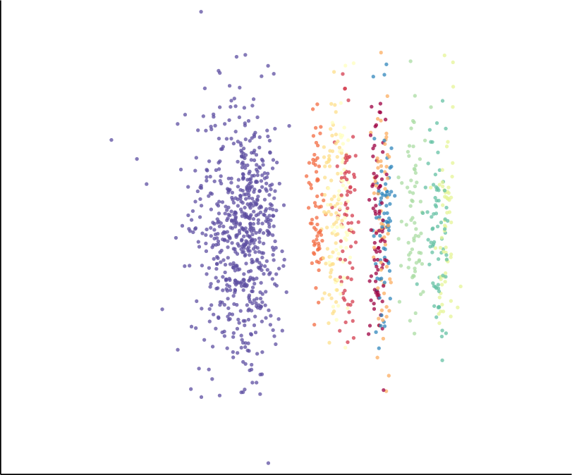
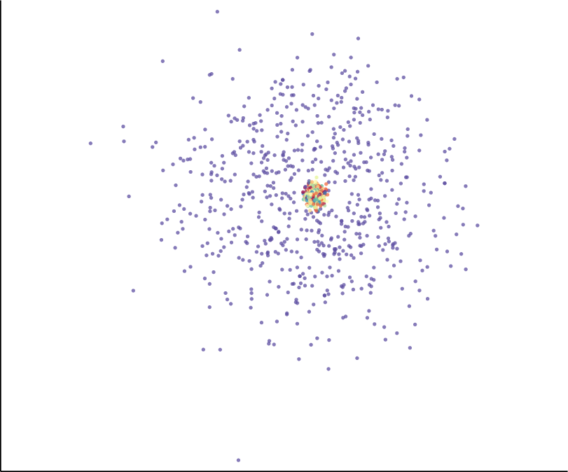
In Figure A.3 we sketch a preliminary experiment, where we apply our topological constraint to variational autoencoders for the Spheres data set. Also here, we observe that our constraint helps identifying the nesting structure of the enclosing sphere.
A.10 Topological Distance Calculations
To assess the topological fidelity of the resulting latent spaces, we calculate several topological distances between the test data set (full dimensionality) and the latent spaces obtained from each method (two dimensions). More precisely, we calculate (i) the st Wasserstein distance (), (ii) the nd Wasserstein distance (), and (iii) the bottleneck distance () between the persistence diagrams obtained from the test data set of the Spheres data and their resulting 2D latent representations. Even though our loss function is not optimising this distance, we observe in Table A.1 that the topological distance of our method (“TopoAE”) is always the lowest among all the methods. In particular, it is always smaller than the topological distance of the latent space of the autoencoder architecture; this is true for all distance measures, even though , for example, is known to be susceptible to outliers. Said experiment serves as a simple “sanity check” as it demonstrates that the changes induced by our method are beneficial in that they reduce the topological distance of the latent space to the original data set. For a proper comparison of topological features between the two sets of spaces, a more involved approach would be required, though.
| Method | |||
|---|---|---|---|
| Isomap | 4.320.037 | 0.4770.0045 | 0.1650.00096 |
| PCA | 4.420.053 | 0.4760.0046 | 0.1580.00108 |
| t-SNE | 4.380.038 | 0.4780.0045 | 0.1640.00094 |
| UMAP | 4.470.042 | 0.4780.0045 | 0.1600.00092 |
| AE | 3.990.037 | 0.4690.0053 | 0.1540.00128 |
| TopoAE | 3.730.076 | 0.4590.0055 | 0.1520.00268 |
A.11 Alternative Loss Formulations
Our choice of loss function was motivated by the observation that only aligning the persistence diagrams between mini-batches of and can lead to degenerate or “meaningless” latent spaces. As a simple example (see Figure A.4 for a visualisation), imagine three non-collinear points in the input space and the triangle they are forming. Now assume that the latent space consists of the same triangle (in terms of its side lengths) but with permuted labels. A loss term of the form
| (30) |
only measures the distance between persistence diagrams (which would be zero in this situation) and would not be able to penalise such a configuration.









| Data set | Method | -Cont | -MRRE | -Trust | -RMSE | Data MSE | |||||
|---|---|---|---|---|---|---|---|---|---|---|---|
| Spheres | Isomap | 0.530950.01929 | 0.180960.02547 | 0.420480.00559 | 0.008810.00020 | 0.0000890.000002 | 0.790270.00244 | 0.245730.00158 | 0.676430.00323 | 10.371880.22856 | – |
| PCA | 0.224450.00691 | 0.332310.00552 | 0.651210.00256 | 0.015300.00010 | 0.0001590.000001 | 0.747400.00140 | 0.294020.00108 | 0.625570.00066 | 11.764820.01460 | 0.961030.00029 | |
| TSNE | 0.227940.00722 | 0.152280.00805 | 0.527220.03261 | 0.012710.00058 | 0.0001330.000006 | 0.773000.00513 | 0.217400.00472 | 0.678620.00474 | 8.050180.11057 | – | |
| UMAP | 0.247520.01917 | 0.156870.00599 | 0.613260.00752 | 0.016580.00028 | 0.0001780.000003 | 0.751530.00360 | 0.249680.00094 | 0.634830.00185 | 9.270090.03417 | – | |
| Vanilla | 0.284320.02165 | 0.565710.02864 | 0.745880.04323 | 0.016640.00115 | 0.0001720.000013 | 0.606630.01685 | 0.349180.00903 | 0.588430.00475 | 13.330610.05198 | 0.815450.00106 | |
| TopoPCA | 0.433440.01823 | 0.178370.00888 | 0.398160.01178 | 0.008660.00025 | 0.0000870.000003 | 0.773200.00135 | 0.327650.00158 | 0.622600.00251 | 11.915420.56134 | 0.973050.00067 | |
| TopoAE | 0.627650.05415 | 0.085040.01270 | 0.325720.02050 | 0.006940.00055 | 0.0000690.000006 | 0.822000.01813 | 0.272390.01108 | 0.657750.01428 | 13.457530.04177 | 0.868120.00074 | |
| F-MNIST | PCA | 0.225590.00011 | 0.355940.00011 | 0.052050.00004 | 0.000690.00000 | 0.0000070.000000 | 0.967770.00001 | 0.057440.00001 | 0.916810.00003 | 9.051210.00041 | 0.184390.00000 |
| TSNE | 0.035160.00226 | 0.404770.01251 | 0.070950.00962 | 0.001980.00026 | 0.0000230.000003 | 0.967310.00268 | 0.019620.00073 | 0.974050.00070 | 41.254600.53671 | – | |
| UMAP | 0.050690.00238 | 0.423620.00609 | 0.064910.00161 | 0.001630.00005 | 0.0000190.000001 | 0.981260.00016 | 0.028670.00034 | 0.958740.00060 | 13.689330.02896 | – | |
| Vanilla | 0.171770.13603 | 0.477980.09567 | 0.067910.00700 | 0.001250.00017 | 0.0000140.000002 | 0.968490.00372 | 0.025620.00217 | 0.974180.00119 | 20.706743.56861 | 0.101970.00222 | |
| TopoPCA | 0.188570.00197 | 0.362010.00186 | 0.052960.00045 | 0.000830.00002 | 0.0000090.000000 | 0.970300.00013 | 0.055840.00022 | 0.917900.00034 | 20.888810.29929 | 0.183150.00002 | |
| TopoAE | 0.110390.02948 | 0.392040.03264 | 0.053530.00959 | 0.001000.00015 | 0.0000110.000002 | 0.979980.00194 | 0.031560.00253 | 0.956120.00391 | 20.491220.93206 | 0.120710.00238 | |
| MNIST | PCA | 0.167540.00051 | 0.388760.00146 | 0.163010.00059 | 0.001600.00001 | 0.0000160.000000 | 0.900840.00016 | 0.165820.00022 | 0.745460.00048 | 13.174370.00216 | 0.222690.00002 |
| TSNE | 0.037670.00140 | 0.276950.05266 | 0.132660.02362 | 0.002140.00041 | 0.0000240.000004 | 0.921010.00288 | 0.039530.00129 | 0.946240.00147 | 22.892610.24373 | – | |
| UMAP | 0.072140.00091 | 0.320630.00320 | 0.145680.00207 | 0.002340.00004 | 0.0000270.000001 | 0.939920.00066 | 0.051090.00022 | 0.937700.00039 | 14.615350.04332 | – | |
| Vanilla | 0.446900.08540 | 0.619930.11742 | 0.155420.02203 | 0.001560.00023 | 0.0000160.000002 | 0.912930.00564 | 0.058280.00353 | 0.936990.00262 | 18.181050.21459 | 0.137320.00160 | |
| TopoPCA | 0.161380.00716 | 0.391570.01283 | 0.155560.00313 | 0.001620.00007 | 0.0000170.000001 | 0.903010.00057 | 0.162970.00049 | 0.750400.00091 | 17.333530.82592 | 0.224770.00009 | |
| TopoAE | 0.324270.03312 | 0.340690.03056 | 0.110120.01069 | 0.001140.00010 | 0.0000120.000001 | 0.932100.00132 | 0.055530.00044 | 0.928440.00142 | 19.577840.01812 | 0.138840.00066 | |
| CIFAR | PCA | 0.273200.00014 | 0.590730.00004 | 0.019610.00001 | 0.000230.00000 | 0.0000020.000000 | 0.931300.00000 | 0.119210.00005 | 0.821170.00002 | 17.715670.00084 | 0.148160.00000 |
| TSNE | 0.044510.00222 | 0.627330.01427 | 0.030140.00333 | 0.000730.00007 | 0.0000090.000001 | 0.903000.00611 | 0.102650.00242 | 0.863250.00151 | 25.610990.11551 | – | |
| UMAP | 0.069340.00202 | 0.616730.00052 | 0.025620.00019 | 0.000500.00001 | 0.0000060.000000 | 0.920450.00013 | 0.126800.00028 | 0.816680.00019 | 33.577850.00796 | – | |
| Vanilla | 0.377370.06507 | 0.668340.02992 | 0.034580.00448 | 0.000620.00021 | 0.0000070.000002 | 0.850720.00429 | 0.132040.00316 | 0.863590.00442 | 36.268270.56159 | 0.140300.00190 | |
| TopoPCA | 0.272070.00619 | 0.584010.00515 | 0.019730.00040 | 0.000240.00001 | 0.0000030.000000 | 0.924390.00115 | 0.126070.00133 | 0.815510.00139 | 30.738481.35231 | 0.150020.00076 | |
| TopoAE | 0.208770.00951 | 0.556420.00412 | 0.018790.00051 | 0.000310.00002 | 0.0000030.000000 | 0.926910.00100 | 0.108090.00210 | 0.845140.00359 | 37.859140.03303 | 0.139750.00171 |