$B_{s}\to D_{s}\ell\nu$ Form Factors for the full $q^{2}$ range from Lattice QCD with non-perturbatively normalized currents

Abstract

We present a lattice QCD determination of the $B_{s}\to D_{s}\ell\nu$ scalar and vector form factors over the full physical range of momentum transfer. The result is derived from correlation functions computed using the Highly Improved Staggered Quark (HISQ) formalism, on the second generation MILC gluon ensembles accounting for up, down, strange and charm contributions from the sea. We calculate correlation functions for three lattice spacing values and an array of unphysically light $b$-quark masses, and extrapolate to the physical value. Using the HISQ formalism for all quarks means that the lattice current coupling to the $W$ can be renormalized non-perturbatively, giving a result free from perturbative matching errors for the first time. Our results are in agreement with, and more accurate than, previous determinations of these form factors. From the form factors we also determine the ratio of branching fractions that is sensitive to violation of lepton universality: $R(D_{s})=\mathcal{B}(B_{s}\to D_{s}\tau\nu_{\tau})/\mathcal{B}(B_{s}\to D_{s}\ell\nu_{l})$, where $\ell$ is an electron or a muon. We find $R(D_{s})=0.2987(46)$, which is also more accurate than previous lattice QCD results. Combined with a future measurement of $R(D_{s})$, this could supply a new test of the Standard Model. We also compare the dependence on heavy quark mass of our form factors to expectations from Heavy Quark Effective Theory.

I Introduction

The weak decay processes of mesons such as the $B$ and $B_{s}$, containing $b$ quarks, are a key potential source of insights into physics beyond the Standard Model (SM). Flavour-changing $B$ decays have gained a lot of interest because of a number of related tensions between experimental measurements and SM predictions Wei et al. (2009); Lees et al. (2012a, b, 2013); Aaij et al. (2014a, b); Huschle et al. (2015); Aaij et al. (2016a, 2015a, 2015b, b); Wehle et al. (2017); Sato et al. (2016); Hirose et al. (2018); Aaij et al. (2018a, b, 2017); Sirunyan et al. (2018); Aaboud et al. (2018). These tensions drive the need for improved theoretical calculations in the SM using methods and studying processes where we have good control of the uncertainties.

Lattice QCD is the method of choice for providing the hadronic input known as form factors that determine, up to a normalisation factor, the differential branching fraction for exclusive decay processes such $B\to D\ell\nu$ (we suppress all electric charge and particle-antiparticle labels here in referring to decay processes). The normalisation factor that can then be extracted by comparison of theory with experiment is the Cabibbo-Kobayashi-Maskawa matrix element, in this case $|V_{cb}|$ Aubert et al. (2009, 2010); Bailey et al. (2015); Na et al. (2015); Glattauer et al. (2016). Determination of $|V_{cb}|$ then feeds into constraints on new physics through, for example, tests of the unitarity triangle.

There has been a long-standing tension in determinations of $|V_{cb}|$ between exclusive (from $B\to D\ell\nu$ and $B\to D^{*}\ell\nu$ decays), and inclusive (from $B\to X_{c}\ell\nu$, where $X_{c}$ is any charmed hadronic state) processes. The most accurate exclusive results came from studies of the $B\to D^{*}\ell\nu$ decay at zero recoil. It now seems likely that the uncertainties there were being underestimated because of the use of a very constrained parameterisation in the extrapolation of the experimental $B\to D^{*}$ data to the zero recoil limit Bernlochner et al. (2017); Bigi et al. (2017a); Grinstein and Kobach (2017); Tanabashi et al. (2018), but see also Lees et al. (2019); Gambino et al. (2019). This underlines the importance in future of comparing theory and experiment across the full range of squared 4-momentum transfer ($q^{2}$) (a point emphasised for $D\to K$ in Koponen et al. (2013)). It also demonstrates the need for comparison of accurate results from multiple decay processes for a more complete picture. Improved methods for producing the theoretical input to $|V_{cb}|_{\text{excl}}$, namely lattice QCD determinations of form factors, are clearly necessary.

Here we provide improved accuracy for the form factors for the $B_{s}\to D_{s}\ell\nu$ decay using a new lattice QCD method that covers the full $q^{2}$ range of the decay for the first time. Preliminary results appeared in McLean et al. (2018). The $B_{s}\to D_{s}$ form factors are more attractive than $B\to D$ for a first calculation to test methodology. They are numerically faster to compute and have higher statistical accuracy and smaller finite-volume effects because no valence $u/d$ quarks are present. Chiral perturbation theory Laiho and Van de Water (2006) expects that the $B\to D$ form factors should be relatively insensitive to the spectator quark mass and hence should be very similar between $B_{s}\to D_{s}$ and $B\to D$. This is confirmed at the 5% level by lattice QCD calculations Bailey et al. (2012); Monahan et al. (2017). Hence improved calculations of $B_{s}\to D_{s}$ form factors can also offer information on $B\to D$.

Given an experimental determination, the $B_{s}\to D_{s}\ell\nu$ decay can supply a new method for precisely determining the Cabibbo-Kobayashi-Maskawa (CKM) element $|V_{cb}|$. It can also supply a new test of the SM through quantities sensitive to lepton universality violation. We give the SM result for $R(D_{s})=\mathcal{B}(B_{s}\to D_{s}\tau\nu_{\tau})/\mathcal{B}(B_{s}\to D_{s}l\nu_{l})$, where $l=e$ or $\mu$. An experimental value for comparison to this would help to clarify the tension found between the SM and experiment in the related ratios $R(D^{(*)})=\mathcal{B}(B\to D^{(*)}\tau\nu_{\tau})/\mathcal{B}(B\to D^{(*)}l\nu_{l})$ Amhis et al. (2017) (see also a preliminary new analysis by Belle Caria (2019)).

Three lattice QCD calculations of $B_{(s)}\to D_{(s)}$ form factors have already been performed. The FNAL/MILC collaboration Bailey et al. (2012, 2015) used the Fermilab action for the $b$ and $c$ quarks and the asqtad action for the light quarks on MILC gluon field ensembles that include $2+1$ flavours of asqtad sea quarks. On the same gluon field ensembles the HPQCD collaboration has calculated the form factors using Nonrelativistic QCD (NRQCD) for the valence $b$ and the Highly Improved Staggered Quark (HISQ) action for the other valence quarks Na et al. (2015); Monahan et al. (2017). A further calculation has been done using maximally twisted Wilson quarks on $n_{f}=2$ gluon field ensembles Atoui et al. (2014). Preliminary results using domain-wall quarks are given in Flynn et al. (2018).

A considerable limitation in the FNAL/MILC and HPQCD/NRQCD studies is the requirement for normalisation of the lattice QCD $b\to{c}$ current. The matching between this current and that of continuum QCD is done in lattice QCD perturbation theory through $\mathcal{O}(\alpha_{s})$, giving a $\mathcal{O}(\alpha_{s}^{2})$ systematic error which can be sizeable. Systematic errors coming from the truncation of the nonrelativistic expansion of the current are also a problem. In the Fermilab formalism the missing terms become $\mathcal{O}(\alpha_{s}a)$ discretisation effects on fine enough lattices; in the NRQCD formalism they mix discretisation effects and $\mathcal{O}(\alpha_{s}/m_{b})$ (where $m_{b}$ is the $b$ quark mass) relativistic corrections. Here we dispense with both of these problems by using a relativistic formalism with absolutely normalised lattice QCD currents.

Another limitation present in each of the previous studies is that the lattice QCD results are limited to a region of high $q^{2}$, close to zero recoil. The reason for this is mainly to avoid large statistical errors. The signal/noise degrades exponentially as the spatial momentum of the meson in the final state grows. For $b$ quark decays the maximum spatial momentum of the final state meson can be large (tending to $m_{B}/2$ for light mesons, where $m_{B}$ is the $B$ meson mass). Systematic errors from missing discretisation (and relativistic) corrections also grow away from zero recoil. This is particularly problematic if discretisation effects are $\mathcal{O}(a)$ as above and relatively coarse lattices are used (to reduce numerical cost). Working close to zero recoil means that the lattice results then have to be extrapolated from the high $q^{2}$ region into the rest of the physical $q^{2}$ range. Here we also overcome this problem by working with a highly improved quark action in which even $\mathcal{O}(a^{2})$ errors have been eliminated at tree-level Follana et al. (2007). We cover a range of values of the lattice spacing that includes very fine lattices and include results from lighter than physical $b$ quarks and this enables us to cover the full $q^{2}$ range in our lattice calculation.

We perform our calculation on the second-generation MILC gluon ensembles Bazavov et al. (2013), including effects from 2+1+1 flavours in the sea using the HISQ action Follana et al. (2007). We also use the HISQ action for all valence quarks. Our calculation employs HPQCD’s heavy-HISQ approach. In this we obtain lattice results at a number of unphysically light masses for the $b$ (we refer to this generically as the heavy quark $h$), reaching the $b$ quark mass on the finest lattices. This allows us to perform a combined fit in $m_{h}$ and lattice spacing that we can evaluate in the continuum limit at $m_{h}=m_{b}$ (and as a function of $m_{h}$ to compare, for example, to expectations from Heavy Quark Effective Theory (HQET)). By using only HISQ quarks, we can normalise all the lattice currents fully non-perturbatively and avoid systematic errors from current matching.

This calculation adds to a growing number of successful demonstrations of the heavy-HISQ approach. The method was developed for determination of the $b$ quark mass, $B$ meson masses and decay constants McNeile et al. (2010, 2012a, 2012b) and is now also being used by other groups for these calculations Bazavov et al. (2018); Petreczky and Weber (2019). A proof-of-principle application of heavy-HISQ to form factors was given for $B_{c}\to\eta_{c}$ and $B_{c}\to J/\psi$ in Lytle et al. (2016); Colquhoun et al. (2016), covering the full $q^{2}$ range for these decays and this work builds on those results. The $B_{s}\to D_{s}^{*}$ axial form factor at zero recoil was calculated using heavy-HISQ in McLean et al. (2019).

This article is structured in the following way: Section II lays out our lattice QCD approach to calculating the form factors and then Section III presents our results, along with several consistency checks and our determination of $R(D_{s})$. We also give curves showing the heavy-quark mass dependence of some features of the form factors that can be compared to HQET. For those simply hoping to use our calculated $B_{s}\to D_{s}$ form factors, Appendix A gives the parameters and covariance matrix required to reconstruct them.

II Calculation Details

II.1 Form Factors

In this section we specify our notation for the form factors and matrix elements. The differential decay rate for $B_{s}\to D_{s}l\nu$ decays is given in the SM by

$${d\Gamma\over dq^{2}}=\eta_{\text{EW}}{G_{F}^{2}|V_{cb}|^{2}\over 24\pi^{3}M_{B_{s}}^{2}}\left(1-{m_{\ell}^{2}\over q^{2}}\right)^{2}|{\bf{p}}_{D_{s}}|\,\,\times$$ (1)

$$\left[\left(1+{m_{\ell}^{2}\over 2q^{2}}\right)M_{B_{s}}^{2}|{\bf{p}}_{D_{s}}|^{2}f_{+}^{s\,2}(q^{2})+\right.$$

$$\hskip 100.00015pt\left.{3m_{\ell}^{2}\over 8q^{2}}(M_{B_{s}}^{2}-M_{D_{s}}^{2})^{2}f_{0}^{s\,2}(q^{2})\right]$$

where $m_{\ell}$ is the mass of the lepton, $\eta_{\text{EW}}$ is the electroweak correction, $q^{2}=(p_{B_{s}}-p_{D_{s}})^{2}$ is the momentum transfer and $f_{0}^{s}(q^{2})$, $f_{+}^{s}(q^{2})$ are the scalar and vector form factors that parameterize the fact that the decay process involves hadrons. We use superscript ‘$s$’ to denote the strange spectator valence quark. The allowed range of $q^{2}$ values if the final states are on-shell is

$$m_{\ell}^{2}\leq q^{2}\leq(M_{B_{s}}-M_{D_{s}})^{2}.$$ (2)

The form factors are determined from matrix elements of the electroweak current between $B_{s}$ and $D_{s}$ states, $\langle D_{s}|(V-A)^{\mu}|B_{s}\rangle$ where $V^{\mu}=\bar{b}\gamma^{\mu}c$ is the vector component and $A^{\mu}=\bar{b}\gamma^{5}\gamma^{\mu}c$ is the axial vector component. In a pseudoscalar-to-pseudoscalar amplitude, only $V^{\mu}$ contributes, since $\langle D_{s}|A^{\mu}|B_{s}\rangle$ does not satisfy the parity invariance of QCD. In terms of form factors, the vector current matrix element is given by

$$\langle D_{s}|V^{\mu}|B_{s}\rangle =f_{+}^{s}(q^{2})\left[p_{B_{s}}^{\mu}+p_{D_{s}}^{\mu}-{M_{B_{s}}^{2}-M_{D_{s}}^{2}\over q^{2}}q^{\mu}\right]$$

$$+f_{0}^{s}(q^{2}){M_{B_{s}}^{2}-M_{D_{s}}^{2}\over q^{2}}q^{\mu}.$$ (3)

Analyticity of this matrix element demands that

$$f_{+}^{s}(0)=f_{0}^{s}(0).$$ (4)

Via the partially conserved vector current relation (PCVC), the form factor $f_{0}^{s}(q^{2})$ is also directly related to the matrix element of the scalar current $S=\bar{b}c$;

$$(m_{b}-m_{c})\langle D_{s}|S|B_{s}\rangle=(M^{2}_{B_{s}}-M^{2}_{D_{s}})f_{0}^{s}(q^{2}).$$ (5)

In our calculation we determine the form factors by computing matrix elements of the temporal vector current $V^{0}$ and the scalar current $S$. The form factors can be extracted from this combination using expressions derived from Eqs. (3) and (5) (once the currents have the correct continuum normalisation - see Section II.4):

$$f_{0}^{s}(q^{2}) ={m_{b}-m_{c}\over M_{B_{s}}^{2}-M_{D_{s}}^{2}}\langle D_{s}|S|B_{s}\rangle,$$

$$f_{+}^{s}(q^{2}) ={1\over 2M_{B_{s}}}{\delta^{M}\langle D_{s}|S|B_{s}\rangle-q^{2}\langle D_{s}|V^{0}|B_{s}\rangle\over{\bf{p}}^{2}_{D_{s}}},$$ (6)

$$(\,\delta^{M}=(m_{b}-m_{c})(M_{B_{s}}-E_{D_{s}})\,).$$

Our goal is to compute $f_{0}^{s}(q^{2})$ and $f_{+}^{s}(q^{2})$ throughout the range of $q^{2}$ values $0\leq q^{2}\leq(M_{B_{s}}-M_{D_{s}})^{2}\equiv q^{2}_{\text{max}}$. We extend the range to $q^{2}=0$ in order to take advantage of the constraint from Equation (4).

set	handle	$w_{0}/a$	$N_{x}^{3}\times N_{t}$	$am_{l0}$	$am_{s0}$	$am_{c0}$
1	fine	1.9006(20)	$32^{3}\times 96$	0.0074	0.037	0.440
2	fine-	1.9518(7)	$64^{3}\times 96$	0.0012	0.0363	0.432
	physical
3	superfine	2.896(6)	$48^{3}\times 144$	0.0048	0.024	0.286
4	ultrafine	3.892(12)	$64^{3}\times 192$	0.00316	0.0158	0.188

Table 1: Parameters for gluon field ensembles Bazavov et al. (2010, 2013). $a$ is the lattice spacing, determined from the Wilson flow parameter $w_{0}$ Borsanyi et al. (2012). Values for $w_{0}/a$ are from: set 1 Chakraborty et al. (2017), sets 2 and 3 Chakraborty et al. (2015), set 4 McNeile (2015). The physical value of $w_{0}$ was determined to be $0.1715(9)$fm in Dowdall et al. (2013). $N_{x}$ is the spatial extent and $N_{t}$ the temporal extent of the lattice in lattice units. Light ($m_{u}=m_{d}$), strange and charm quarks are included in the sea, their masses are given in columns 5-7.

set	$am_{s0}^{\text{val}}$	$am_{c0}^{\text{val}}$	$am^{\text{val}}_{h0}$	$|a{\bf{p}}_{D_{s}}|$	$n_{\text{cfg}}\times n_{\text{src}}$	$T$
1	0.0376	0.45	0.5	0, 0.056	$986\times 8$	14, 17, 20
			0.65	0, 0.142, 0.201
			0.8	0, 0.227, 0.323
2	0.036	0.433	0.5	0, 0.0279	$286\times 4$	14, 17, 20
			0.8	0, 0.162
3	0.0234	0.274	0.427	0, 0.113, 0.161	$250\times 8$	22, 25, 28
			0.525	0, 0.161, 0.244
			0.65	0, 0.244, 0.338
			0.8	0, 0.338, 0.438
4	0.0165	0.194	0.5	0, 0.202, 0.281	$237\times 4$	31, 36, 41
			0.65	0, 0.202, 0.281, 0.382
			0.8	0, 0.281, 0.382, 0.473

Table 2: Calculational details. Columns 2 and 3 give the $s$ and $c$ valence quark masses in lattice units, which were tuned in Chakraborty et al. (2015). In column 4 we give the heavy quark masses that we used in lattice units. We use a number of heavy quark masses to enable the heavy-quark mass dependence to be determined in our fit. Column 5 gives the absolute value of the spatial momentum (in lattice units) given to the $D_{s}$ meson using a momentum twist on the charm quark propagator. These values are chosen with the following rationale: when only two values are given, these correspond to the $q^{2}=0$ and $q^{2}_{\text{max}}$ points (except on the fine-physical ensemble, where we use the points $q^{2}_{\text{max}}$ and $q^{2}_{\text{max}}/2$); when three values are given, the momenta correspond to $q^{2}=0$, $q^{2}=q^{2}_{\text{max}}/2$, and $q^{2}_{\text{max}}$; when four values are given, these are points corresponding to $q^{2}_{\text{max}}$, $3q^{2}_{\text{max}}/4$, $q^{2}_{\text{max}}/2$, $q^{2}_{\text{max}}/4$ and $q^{2}=0$. We used twisted momenta in the $(1,1,1)$ direction to minimise discretisation effects. Column 6 gives the number of gluon field configurations used for that ensemble, $n_{\text{cfg}}$, and the number of different time sources used per configuration to increase statistics, $n_{\text{src}}$. Column 7 gives the temporal separations between source and sink, $T$, of the three-point correlation functions computed on each ensemble.

II.2 Lattice Calculation

This calculation closely follows the approach employed in our calculation of the $B_{s}\to D_{s}^{*}$ axial form factor at zero recoil McLean et al. (2019). Here, however, we must give spatial momentum to the charm quark in the final state so that we can cover the full $q^{2}$ range of the decay.

The gluon field configurations used in this calculation were generated by the MILC collaboration Bazavov et al. (2010, 2013). The relevant parameters for the specific ensembles we use are given in Table 1. The gluon fields are generated using a Symanzik-improved gluon action with coefficients matched to continuum QCD through $\mathcal{O}(\alpha_{s}a^{2},n_{f}\alpha_{s}a^{2})$ Hart et al. (2009). The gluon fields include the effect of 2+1+1 flavours of quarks in the sea ($u$, $d$, $s$, $c$, where $m_{u0}=m_{d0}\equiv m_{l0}$) using the HISQ action Follana et al. (2007). In three of the four ensembles (sets 1, 3 and 4), the bare light quark mass is set to $m_{l0}/m_{s0}=0.2$. The fact that the $m_{l0}$ value is unphysically high is expected to have only a small effect on the form factors here, since we have no valence light quarks. We quantify this small effect by including a fourth ensemble (set 2) with roughly physical $m_{l0}$.

We use a number of different masses for the valence heavy quark $am_{h0}^{\text{val}}$. This allows us to resolve the dependence of the form factors on the heavy quark mass, so that a fit in $m_{h}$ can be performed and the results of the fit evaluated at $m_{h}=m_{b}$. With a heavy quark mass varying both on a given ensemble and between ensembles, we can resolve both the discretisation effects that grow with large ($am^{\text{val}}_{h0}\lesssim 1$) masses and the physical dependence of the continuum form factors on $m_{h}$. Using unphysically light $h$-quarks also reduces the $q^{2}$ range, meaning that we can obtain lattice results across the full range while the statistical noise remains under control.

Staggered quarks have no spin degrees of freedom. Spin-parity quantum numbers are accounted for by construction of appropriate fermion bilinears and including an appropriate space-time dependent phase with each operator in the path integral. We categorize these phases according to the standard spin-taste notation, $(\gamma_{n}\otimes\gamma_{s})$, where $\gamma_{n}$ is the spin structure of the operator in the continuum limit, and $\gamma_{s}$ is the ‘taste’ structure which accounts for the multiple possible copies of the operator constructed from staggered quark fields.

We have designed this calculation to use only local operators (combining fields at the same space-time point and having $(\gamma_{n}\otimes\gamma_{n})$ spin-taste) for the calculation of the current matrix elements that we require. This is an advantage since point-split operators can lead to noisier correlation functions. The spin-taste operators we use are: scalar $(1\otimes 1)$, pseudoscalar $(\gamma^{5}\otimes\gamma^{5})$, vector $(\gamma^{\mu}\otimes\gamma^{\mu})$, and temporal axial-vector $(\gamma^{0}\gamma^{5}\otimes\gamma^{0}\gamma^{5})$.

We compute a number of correlation functions on the ensembles detailed in Table 1. Valence quark masses, momenta and other inputs to the calculation are given in Table 2. We use random wall sources to generate all staggered propagators from the source since this gives improved statistical errors Davies et al. (2010a). First we compute two-point correlation functions between meson eigenstates of momentum $a{\bf{p}}$,

$$C^{a{\bf{p}}}_{M}(t) =\frac{1}{N_{\text{taste}}}\langle\tilde{\Phi}_{M}({\bf{p}},t)\tilde{\Phi}_{M}^{\dagger}({\bf{p}},0)\rangle,$$ (7)

$$\tilde{\Phi}_{M}({\bf{p}},t) =\sum_{{\bf{x}}}e^{-i\bf{p}\cdot\bf{x}}\bar{q}({\bf{x}},t)\Gamma q^{\prime}({\bf{x}},t),$$

where $\langle\rangle$ represents a functional integral over all fields, $q,q^{\prime}$ are valence quark fields of the flavours the $M$ meson is charged under, $\Gamma$ is the spin-taste structure of $M$ and the division by the number of tastes is required to normalise closed loops made from staggered quarks Follana et al. (2007). We compute these correlation functions for all $t$ values, i.e. $0\leq t\leq N_{t}$.

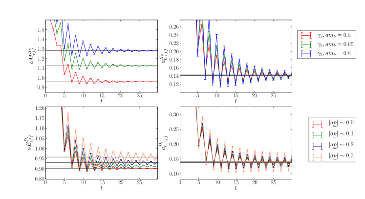
Figure 1: Effective energies and amplitudes, defined from Eqs. (17) and (19) on the fine ensemble. Grey lines show the fit result for the ground-state energies and amplitudes.

Set	$am_{h}^{\text{val}}$	$aM_{H_{s}}$	$aM_{D_{s}}$	$aM_{H_{c}}$	$af_{H_{c}}$	$aM_{\eta_{h}}$	$aM_{\eta_{c}}$	$aM_{\eta_{s}}$
1	0.5	0.95971(12)	0.90217(11)	1.419515(41)	0.186299(70)	1.471675(38)	1.367014(40)	0.313886(75)
	0.65	1.12507(18)		1.573302(40)	0.197220(77)	1.775155(34)
	0.8	1.28129(19)		1.721226(39)	0.207068(78)	2.064153(30)
2	0.5	0.95446(13)	0.87715(11)	1.400025(26)	0.183482(46)	1.470095(25)	1.329291(27)	0.304826(52)
	0.8	1.27560(24)		1.702438(24)	0.203382(50)	2.062957(19)
3	0.427	0.77443(17)	0.59151(11)	1.067224(46)	0.126564(70)	1.233585(41)	0.896806(48)	0.207073(96)
	0.525	0.88470(21)		1.172556(46)	0.130182(72)	1.439515(37)
	0.65	1.01973(28)		1.303144(46)	0.133684(75)	1.693895(33)
	0.8	1.17436(40)		1.454205(46)	0.137277(79)	1.987540(30)
4	0.5	0.80235(19)	0.439899(86)	1.011679(25)	0.099031(45)	1.342747(27)	0.666754(39)	0.153827(77)
	0.65	0.96344(27)		1.169780(26)	0.100598(49)	1.650264(23)
	0.8	1.11728(35)		1.321660(28)	0.101765(54)	1.945763(21)

Table 3: Parameters determined from our correlation function fits. The decay constant $af_{H_{c}}$ is extracted from the amplitude obtained via Eqs. (21) and (22). $D_{s}$ energies at non-zero spatial momentum are given in Table 4.

Set	$am_{h}^{\text{val}}$	$q^{2}$[GeV2]	$aE_{D_{s}}$	$f^{s}_{0}(q^{2})$	$f^{s}_{+}(q^{2})$	$f^{s}_{0}(q^{2})/f_{H_{c}}\sqrt{M_{H_{c}}}$	$f^{s}_{+}(q^{2})/f_{H_{c}}\sqrt{M_{H_{c}}}$
1	0.5	0.01584(17)	0.90217(11)	1.0009(14)		1.394(11)
		0.00026(50)	0.90386(11)	0.9997(14)	0.9997(15)	1.393(11)	1.393(11)
	0.65	0.2376(26)	0.90217(11)	1.0047(28)		1.256(11)
		0.1201(15)	0.91308(13)	0.9956(31)	1.0014(77)	1.245(11)	1.252(14)
		0.0027(12)	0.92399(15)	0.9878(31)	0.9880(32)	1.235(11)	1.235(11)
	0.8	0.6874(74)	0.90217(11)	1.0092(17)		1.1488(94)
		0.3473(40)	0.92992(17)	0.9898(18)	1.0079(56)	1.1267(93)	1.147(11)
		0.0082(29)	0.95759(27)	0.9710(18)	0.9714(19)	1.1053(91)	1.1057(91)
2	0.5	0.03014(32)	0.87715(11)	1.0004(15)		1.369(11)
		0.02593(49)	0.87759(11)	1.0001(15)	1.002(19)	1.369(11)	1.371(28)
	0.8	0.8007(84)	0.87715(11)	1.0054(18)		1.1258(91)
		0.6126(66)	0.89178(15)	0.9948(22)	1.030(18)	1.1139(91)	1.154(22)
3	0.427	0.3715(42)	0.59151(11)	0.9942(24)		1.250(11)
		0.1877(26)	0.60220(14)	0.9807(26)	0.9928(61)	1.233(11)	1.248(13)
		0.0053(23)	0.61281(17)	0.9685(26)	0.9688(26)	1.218(11)	1.218(11)
	0.525	0.954(11)	0.59151(11)	0.9876(25)		1.152(10)
		0.5361(66)	0.61281(17)	0.9614(27)	0.9901(80)	1.121(10)	1.155(13)
		0.0124(54)	0.63946(31)	0.9320(31)	0.9326(31)	1.0870(99)	1.0876(99)
	0.65	2.036(23)	0.59151(11)	0.9791(28)		1.0548(95)
		0.950(12)	0.63946(31)	0.9227(37)	0.9611(81)	0.9940(93)	1.035(12)
		0.007(13)	0.68113(58)	0.8821(42)	0.8823(41)	0.9503(92)	0.9505(92)
	0.8	3.772(43)	0.59151(11)	0.9709(37)		0.9643(90)
		1.435(22)	0.68113(58)	0.8731(53)	0.9138(93)	0.8671(90)	0.908(12)
		-0.030(44)	0.7373(17)	0.825(10)	0.8242(97)	0.819(12)	0.819(12)
4	0.5	2.634(32)	0.439899(86)	0.9741(28)		1.0319(99)
		1.179(16)	0.48514(23)	0.9134(32)	0.9522(63)	0.9676(95)	1.009(11)
		-0.027(18)	0.52261(54)	0.8666(45)	0.8657(44)	0.9181(96)	0.9172(96)
	0.65	5.497(67)	0.439899(86)	0.9575(34)		0.9287(91)
		3.748(47)	0.48514(23)	0.8985(39)	1.004(18)	0.8714(88)	0.974(19)
		2.301(35)	0.52261(54)	0.8529(55)	0.913(11)	0.8272(92)	0.886(13)
		0.198(93)	0.5770(24)	0.770(15)	0.775(14)	0.746(16)	0.751(15)
	0.8	9.20(11)	0.439899(86)	0.9433(40)		0.8508(86)
		5.495(72)	0.52261(54)	0.8438(67)	0.974(23)	0.7611(92)	0.878(22)
		3.06(11)	0.5770(24)	0.768(16)	0.842(23)	0.693(15)	0.759(22)
		0.19(26)	0.6410(57)	0.721(27)	0.724(25)	0.650(25)	0.653(23)

Table 4: Parameters from our correlation function fits at varying $q^{2}$ points. $f_{0,+}^{s}(q^{2})$ are extracted via (23) and (25), and $R^{s}_{0,+}(q^{2})$ is defined in (26). We show statistical/fit errors on each of the quantities, including the value of $q^{2}$ that is derived from $M_{H_{s}}$ and $E_{D_{s}}$. $q^{2}$ and $R^{s}$ uncertainties also include those from the determination of the lattice spacing.

We compute correlation functions for a heavy-strange pseudoscalar, $H_{s}$, with spin-taste structure $(\gamma^{5}\otimes\gamma^{5})$, at rest. In terms of staggered quark propagators this takes the form

$$C_{H_{s}}(t)=\frac{1}{4}\sum_{\bf{x},\bf{y}}\langle\text{Tr}\left[g_{h}(x,y)g_{s}^{\dagger}(x,y)\right]\rangle,$$ (8)

where $g_{q}(x,y)$ is a staggered propagator for flavour $q$, and the trace is over color. Here $x_{0}=0$ and $y_{0}=t$, and the sum is over spatial sites labelled $\bf{x}$, $\bf{y}$. We also compute correlators for a charm-strange pseudoscalar meson $D_{s}$, with structure $(\gamma^{5}\otimes\gamma^{5})$. For these correlators we need both zero and non-zero spatial momentum. Non-zero spatial momentum is given to the $D_{s}$ by imposing twisted boundary conditions on the gluon fields when computing the charm quark propagators Guadagnoli et al. (2006). Then

$$C^{a\bf{p}}_{D_{s}}(t)=\frac{1}{4}\sum_{\bf{x},\bf{y}}\langle\text{Tr}\left[g^{\theta}_{c}(x,y)g_{s}^{\dagger}(x,y)\right]\rangle,$$ (9)

where $g_{q}^{\theta}(x,y)$ denotes a propagator with momentum twist $\theta$. We compute these correlation functions using several different twists to produce the range of momenta given in Table 2. We design the $c$ propagators to have momentum $a{\bf{p}}=|a{\bf{p}}|(1,1,1)$, by imposing a twist $\theta=N_{x}|a{\bf{p}}|/\pi\sqrt{3}$ in each spatial direction.

Necessary for extracting the vector current matrix element, we also compute correlation functions for a non-goldstone pseudoscalar heavy-strange mesons at rest, denoted $\hat{H}_{s}$. This has spin-taste structure $(\gamma^{0}\gamma^{5}\otimes\gamma^{0}\gamma^{5})$. $\hat{H}_{s}$ correlators are computed using

$$C_{\hat{H}_{s}}(t)=\frac{1}{4}\sum_{\bf{x},\bf{y}}\langle(-1)^{\bar{x}_{0}+\bar{y}_{0}}\text{Tr}\left[g_{h}(x,y)g^{\dagger}_{s}(x,y)\right]\rangle,$$ (10)

where we use the notation $\bar{z}_{\mu}=\sum_{\nu\neq\mu}z_{\nu}$.

We also compute correlators for $H_{c}$ mesons, heavy-charmed pseudoscalars, using the same form as those for $H_{s}$, Equation (8). These are used to find $H_{c}$ decay constants, which are useful in some of our continuum and $m_{h}$ fits. In our fits to heavy-quark mass dependence we will use the mass of the heavy-heavy pseudoscalar meson, $\eta_{h}$ as a physical proxy for the quark mass. To quantify mistuning of the charm and strange quark masses, we also require masses for $\eta_{c}$ and $\eta_{s}$ mesons, identical to $\eta_{h}$ with $h$ replaced $c$ and $s$ quarks respectively. We compute correlators for each of these at rest, using a spin-taste structure $(\gamma^{5}\otimes\gamma^{5})$, taking the same form as those of the $H_{s}$, Equation (8). Note that all of the $\eta$ mesons discussed here are artificially forbidden to annihilate in our lattice QCD calculation. We expect this to have negligible effect, for the purposes of this calculation, on the masses of the $\eta_{c}$ and the $\eta_{b}$ Chakraborty et al. (2015); the $\eta_{s}$ is an unphysical meson that can be defined in this limit in a lattice QCD calculation and is convenient for tuning the $s$ quark mass Davies et al. (2010b); Dowdall et al. (2013).

Three-point correlation functions are needed to allow determination of the current matrix elements for $B_{s}\to D_{s}$ decay. We require two sets of such correlation functions, one with a scalar and one with a temporal vector current insertion. The first takes the form

$$C^{a{\bf{p}}_{D_{s}}}_{S}(t,T) =\frac{1}{N_{\text{taste}}}\sum_{{\bf{y}}}\langle\tilde{\Phi}_{D_{s}}({\bf{p}},T)\,S({\bf{y}},t)\,\tilde{\Phi}_{H_{s}}({\bf{0}},0)\rangle,$$ (11)

$$S({\bf{y}},t) =\bar{c}({\bf{y}},t)h({\bf{y}},t).$$

In terms of the staggered quark formalism, both the $H_{s}$ source and $D_{s}$ sink are given structure $(\gamma^{5}\otimes\gamma^{5})$, and the current insertion $(1\otimes 1)$. We combine staggered propagators to construct these correlation functions as:

$$C^{a{\bf{p}}_{D_{s}}}_{S}(t,T)= \frac{1}{4}\sum_{{\bf{x},\bf{y},\bf{z}}}\langle\text{Tr}\left[g_{h}(x,y)g^{\theta}_{c}(y,z)g^{\dagger}_{s}(x,z)\right]\rangle,$$ (12)

where we fix $x_{0}=0$, $y_{0}=t$ and $z_{0}=T$, and once again the charm propagator is given the appropriate twist $\theta$. We compute these correlation functions for all $t$ values within $0\leq t\leq T$, using 3 $T$ values to make sure that excited state effects are accounted for. The $T$ values vary with lattice spacing to give approximately the same physical range and always include both even and odd values. The values are given in Table 2.

The three-point correlation function with temporal vector current insertion is given by

$$C^{a{\bf{p}}_{D_{s}}}_{V^{0}}(t,T) =\frac{1}{N_{\text{taste}}}\sum_{{\bf{y}}}\langle\tilde{\Phi}_{D_{s}}({\bf{p}},T)\,V^{0}({\bf{y}},t)\,\tilde{\Phi}_{\hat{H}_{s}}({\bf{0}},0)\rangle,$$

$$V^{0}({\bf{y}},t) =\bar{c}({\bf{y}},t)\gamma^{0}h({\bf{y}},t).$$ (13)

This is generated using spin-taste $(\gamma^{0}\gamma^{5}\otimes\gamma^{0}\gamma^{5})$ at the $\hat{H}_{s}$ source, $(\gamma^{5}\otimes\gamma^{5})$ at the $D_{s}$ sink, and $(\gamma^{0}\otimes\gamma^{0})$ at the current insertion. To achieve this we compute

$$C^{a{\bf{p}}_{D_{s}}}_{V_{0}}(t,T)= \frac{1}{4}\sum_{{\bf{x},\bf{y},\bf{z}}}\langle(-1)^{\bar{x}_{0}+\bar{y}_{0}}$$

$$\times\text{Tr}\left[g_{h}(x,y)g^{\theta}_{c}(y,z)g^{\dagger}_{s}(x,z)\right]\rangle.$$ (14)

The non-goldstone $\hat{H}_{s}$ is required here to ensure that taste cancels in the correlation function. The difference between the $\hat{H}_{s}$ and the $H_{s}$, for example in their masses, is generated by taste-exchange discretisation effects. In practice it is very small for heavy mesons Follana et al. (2007), being suppressed by the heavy meson mass.

II.3 Analysis of Correlation Functions

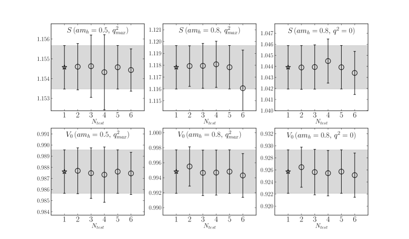
Figure 2: Tests on the correlator fits on the fine ensemble. The y-axis shows the best fit result for $J_{00}^{nn}$, with the appropriate current, heavy mass and $q^{2}$ specified. At $N_{\text{test}}=1$ we give our final result, reproduced by the light grey band for ease of comparison. $N_{\text{test}}=2$ and $3$ give the results of setting $N_{\text{exp}}=4$ and $6$ respectively. $N_{\text{test}}=4$ gives the result of setting $t_{\text{cut}}=3$ for all 2-point correlators (in the final fit $t_{\text{cut}}=2$ for all correlators). $N_{\text{test}}=5$ gives the value when the prior width on the $J_{00}^{nn}$ parameters is doubled. $N_{\text{test}}=6$ gives the results from the output from a fit to the appropriate correlators from that heavy mass and $q^{2}$ value only, and therefore not including correlation with results from other masses and momentum values.

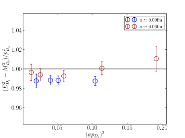
Figure 3: A comparison of the relativistic dispersion relation for our $D_{s}$ mesons on gluon field ensemble sets 1 and 3. We plot the square of the ‘speed of light’ against the square of the spatial momentum of the $D_{s}$ in lattice units. Values on the coarser lattices, set 1, show a small deviation from 1 that is reduced on the finer lattices.

We now describe our simultaneous multi-exponential fits to the correlation functions using a standard Bayesian apporach Lepage et al. (2002); cor (2018). The parameters that we wish to determine are ground-state energies, two-point amplitudes and ground-state to ground-state matrix elements. Our correlation functions, however, are contaminated by contributions from excited states. These excited states must be included in our fits so that the systematic error on the ground-state parameters from the presence of the excited states is fully taken into account. Multi-exponential fits are then mandatory, guided by Bayesian priors for the parameters, discussed below. To reduce the number of exponentials needed by the fits, we drop values of the correlation functions when they are within $t_{\text{cut}}$ of the end-points (where excited states contribute most). We use values of $t_{\text{cut}}$ varying from 2 to 10 throughout the correlator fits. We take results from fits using 5 exponentials ($N_{\text{exp}}=5$ in the fit forms below), where good $\chi^{2}$ values are obtained and the ground-state parameters and their uncertainties have stabilised.

Two-point correlation functions are fit to the form

$$C_{M}(t)|_{\text{fit}}= \sum_{n}^{N_{\text{exp}}}\Big{(}|a^{M}_{n}|^{2}f(E^{M}_{n},t)$$

$$-(-1)^{t}|a^{M,o}_{n}|^{2}f(E_{n}^{M,o},t)\Big{)},$$ (15)

where

$$f(E,t)=\left(e^{-Et}+e^{-E(N_{t}-t)}\right),$$ (16)

and $E^{M,(o)}_{n}$,$a^{M,(o)}_{n}$ are fit parameters. The second term in Equation (II.3) accounts for the opposite-parity states that arise from the staggered quark time doublers and are known as oscillating states (see Appendix G of Follana et al. (2007)). These oscillating states do not appear when $M$ is a Goldstone-taste pseudoscalar with a quark and antiquark of the same mass, so in the $M=\eta_{h},\eta_{c},$ and $\eta_{s}$ cases the second term is not required.

Figure 1 shows the quality of our results. We plot effective energies and amplitudes for the $D_{s}$ and $H_{s}$ mesons on the fine ensemble. The effective energy is defined as

$$E_{\text{eff}}(t)=-\log\left(\frac{\tilde{C}(t)}{\tilde{C}(t-1)}\right).$$ (17)

Here $\tilde{C}$ is a time-smeared mean correlator to reduce the impact of the oscillating states:

$$\tilde{C}(t)=C(t-1)+2C(t)+C(t+1),$$ (18)

where $C(t)$ is defined in Equations (8) and (9). At large $t$ we expect $E_{\text{eff}}(t)$ to stabilise at the ground-state energy and we see that happening in Figure 1. An effective amplitude can then be defined from

$$a_{\text{eff}}(t)=\sqrt{\tilde{C}(t)e^{E_{\text{eff}}(t)t}}/[2\cosh(E_{\text{eff}}/2)]$$ (19)

This again converges to the ground-state amplitude from the fit.

For the three-point correlation functions we use the fit form

$$C_{J} (t,T)|_{\text{fit}}=$$ (20)

$$\sum_{k,j=0}^{N_{\text{exp}},N_{\text{exp}}}\Big{(}\,a^{\mathord{\mathop{H}\limits^{\scriptscriptstyle(\wedge)}}_{s}}_{j}J^{nn}_{jk}a^{D_{s}}_{k}f(E^{H_{s}},t)f(E^{D_{s}}_{n},T-t)$$

$$+a^{\mathord{\mathop{H}\limits^{\scriptscriptstyle(\wedge)}}_{s},o}_{j}J^{on}_{jk}a^{D_{s}}_{k}(-1)^{t}f(E^{\mathord{\mathop{H}\limits^{\scriptscriptstyle(\wedge)}}_{s},o}_{n},t)f(E^{D_{s}},T-t)$$

$$+a^{\mathord{\mathop{H}\limits^{\scriptscriptstyle(\wedge)}}_{s}}_{j}J^{no}_{jk}a^{D_{s},o}_{k}(-1)^{T-t}f(E^{\mathord{\mathop{H}\limits^{\scriptscriptstyle(\wedge)}}_{s}},t)f(E^{D_{s}^{*},o}_{n},T-t)$$

$$+a^{\mathord{\mathop{H}\limits^{\scriptscriptstyle(\wedge)}}_{s},o}_{j}J^{oo}_{jk}a^{D_{s},o}_{k}(-1)^{T}f(E^{\mathord{\mathop{H}\limits^{\scriptscriptstyle(\wedge)}}_{s},o}_{n},t)f(E^{D_{s},o},T-t)\,\Big{)}.$$

This includes fit parameters common to the fits of $H_{s}$ (when $J=S$), $\hat{H}_{s}$ (when $J=V_{0}$) and $D_{s}$ two-point correlators, along with new fit parameters $J_{jk}$ that are related to the current matrix elements. We perform a single simultaneous fit containing each correlator computed ($C_{H_{s}},C_{\hat{H}_{s}},C_{D_{s}},C_{\eta_{h}},C_{\eta_{c}},C_{\eta_{s}},C_{H_{c}},C_{S},C_{V_{0}}$) at every $am_{h}$ and every $|a{\bf{p}}_{D_{s}}|$, for each ensemble.

These simultaneous fits are very large and this causes problems for the covariance matrix which must be inverted to determine $\chi^{2}$. We take two steps toward mitigating this. The first is to impose an svd (singular value decomposition) cut $c_{\text{svd}}$. This replaces any eigenvalue of the covariance matrix smaller than $c_{\text{svd}}x$ with $c_{\text{svd}}x$, where $x$ is the largest eigenvalue of the matrix. The small eigenvalues are driven to zero if the statistics available are not high enough. The application of the svd cut makes the matrix less singular, and can be considered a conservative move since the only possible effect on the error of the final results is to inflate them. An appropriate value for $c_{\text{svd}}$ is found by comparing estimates of covariance matrix eigenvalues between different bootstrap samples of the data using the Corrfitter package cor (2018). The resulting $c_{\text{svd}}$ varies between ensembles since it depends on the statistical quality of the dataset, but we find them to be of order $10^{-3}$.

The other step we take towards a stable fit is employing a chained-fitting approach. We first perform an array of smaller fits, each fitting the correlators relevant only to one $m_{h}$ and one $|a{\bf{p}}_{D_{s}}|$ value. In the case of set 4, for example, this results in 11 separate fits. Then, a full simultaneous fit of all of the correlators is carried out, using as priors the results of the smaller fits. This both speeds up the full fit and improves stability of the results.

The priors for the fits were set up as follows. We set gaussian priors for the parameters $J_{jk}$, and log-normal priors for amplitudes $a_{i}^{M}$, ground-state energies $E_{0}^{M}$, and excited-state energy differences $E_{i+1}^{M}-E_{i}^{M}$. Using log-normal distributions forbids ground-state energies, excited state energy differences and amplitudes moving too close to zero or becoming negative, improving stability of the fit.

Priors for ground state energies $E_{0}^{M}$ and amplitudes $a_{0}^{M}$ are set according to an empirical-Bayes approach, plots of the effective amplitude of the correlation functions are inspected to deduce reasonable priors. The ground-state oscillating parameters $a_{0}^{M,o}$, $E_{0}^{M,o}$, are given the same priors as the non-oscillating states, with uncertainties inflated by 50%. The resulting priors always have a standard deviation at least 10 times that of the final result. The logs of the excited-state energy differences are given prior values $2a\Lambda_{\text{QCD}}\pm a\Lambda_{\text{QCD}}$ where $\Lambda_{\text{QCD}}$ was taken as 0.5 GeV. The log of oscillating and non-oscillating excited state amplitudes are given priors of $-1.9\pm 3.3$. The ground-state non-oscillating to non-oscillating three-point parameter, $J_{00}^{nn}$ is given a prior of $1\pm 0.5$, and the rest of the three-point parameters $J_{jk}^{nn}$ are given $0\pm 1$.

The physical quantities that we need here are extracted from the ground-state fit parameters and given in Tables 3 and 4. $E_{0}^{M}$ are the ground-state meson energies in lattice units. For mesons at rest, this corresponds to the mass of the meson, i.e. $E_{0}^{M}=aM_{M}$. The annihilation amplitude for an $M$-meson at rest is given in lattice units by

$$\langle 0|\tilde{\Phi}_{M}|M\rangle|_{\text{lat}}=\sqrt{2M_{M}}a_{0}^{M}.$$ (21)

If $\tilde{\Phi}_{M}$ is a $\gamma_{5}\otimes\gamma_{5}$ pseudoscalar operator $P$, the decay constant can be found from this via

$$f_{M}={m^{\text{val}}_{q0}+m^{\text{val}}_{q^{\prime}0}\over M_{M}^{2}}\langle\Omega|P|M\rangle|_{\text{lat}},$$ (22)

where $q$,$q^{\prime}$ are the quark flavours that $M$ is charged under. We use this to determine the $H_{c}$ meson decay constant in Table 3. The current matrix elements that we are focussed on here can be extracted from the fit parameters via

$$\langle D_{s}|J|H_{s}\rangle|_{\text{lat}}=2\sqrt{M_{H_{s}}E_{D_{s}}}J^{nn}_{00}.$$ (23)

These can be converted into values for the form factors once the currents have been normalised (Section II.4).

Figure 2 shows the results of a number of tests we performed on the fits to correlators on the fine ensemble. Each test modifies one of the features of the fits and we then plot the resultant value of the key output parameter $J_{00}^{nn}$. The robustness of the fits can be gauged by the effect of these changes, which are all small.

Figure 3 shows a comparison of the $D_{s}$ meson dispersion relation on the fine (set 1) and superfine (set 3) lattices. The dispersion relation is sensitive to discretisation effects in our quark action. The figure shows them to be small (see Donald et al. (2012) for more discussion of discretisation effects in dispersion relations for mesons using HISQ quarks).

Set	$am_{h0}^{\text{val}}$	$Z_{V}$	$Z_{\text{disc}}$
1	0.5	1.0155(23)	0.99819
	0.65	1.0254(35)	0.99635
	0.8	1.0372(32)	0.99305
2	0.5	1.0134(24)	0.99829
	0.8	1.0348(29)	0.99315
3	0.427	1.0025(31)	0.99931
	0.525	1.0059(33)	0.99859
	0.65	1.0116(37)	0.99697
	0.8	1.0204(46)	0.99367
4	0.5	1.0029(38)	0.99889
	0.65	1.0081(43)	0.99704
	0.8	1.0150(49)	0.99375

Table 5: Normalization constants applied to the lattice currents in Equation (25). $Z_{V}$ is found from Equation (24) and $Z_{\text{disc}}$ from McLean et al. (2019).

II.4 Current Normalization

In the HISQ formalism, the local scalar current $(1\otimes 1)$ (multiplied by the mass difference of flavours it is charged under) is conserved, and hence requires no renormalization. This is not the case for the local temporal vector current $(\gamma^{0}\otimes\gamma^{0})$. We use this instead of the conserved vector current because it is much simpler, but we then require a renormalisation factor to match to the continuum current. This is simple to obtain fully non-perturbatively within this calculation Koponen et al. (2013); Donald et al. (2014), at no additional cost.

When both meson states in the matrix elements are at rest (the zero recoil point), the scalar and local vector matrix elements are related via the PCVC relation:

$$(M_{H_{s}} -M_{D_{s}})Z_{V}\langle D_{s}|V^{0}|\hat{H}_{s}\rangle|_{\text{lat}}$$

$$=(m^{\text{val}}_{h0}-m^{\text{val}}_{c0})\langle D_{s}|S|H_{s}\rangle|_{\text{lat}}.$$ (24)

$Z_{V}$ can be extracted from this relation using the matrix elements we have computed. The $Z_{V}$ values found on each ensemble and for each $am^{\text{val}}_{h0}$ are given in Table 5.

We also remove $\mathcal{O}(am_{h}^{4})$ tree-level mass-dependent discretisation effects from the current using a normalization constant, $Z_{\text{disc}}$ derived in Monahan et al. (2013) and discussed in detail in McLean et al. (2019). $Z_{\text{disc}}$ values are also tabulated in Table 5; they have only a very small effect.

Combining these normalizations with the lattice current from the simultaneous correlation function fits, we find values for the form factors at a given heavy mass, lattice spacing, and $q^{2}$:

$$f_{0}^{s} (q^{2})={m^{\text{val}}_{h0}-m^{\text{val}}_{c0}\over M_{H_{s}}^{2}-M_{D_{s}}^{2}}Z_{\text{disc}}\langle D_{s}|S|H_{s}\rangle|_{\text{lat}}(q^{2})$$

$$f_{+}^{s} (q^{2})={Z_{\text{disc}}\over 2M_{H_{s}}}\times$$ (25)

$${\delta^{M}\langle D_{s}|S|B_{s}\rangle|_{\text{lat}}(q^{2})-q^{2}Z_{V}\langle D_{s}|V^{0}|B_{s}\rangle|_{\text{lat}}(q^{2})\over{\bf{p}}^{2}_{D_{s}}}.$$

where $\delta^{M}$ is defined in Equation (II.1) and we have made the dependence of the matrix elements on $q^{2}$ explicit.

II.5 Obtaining a result at the Physical Point

We now discuss how we fit our results for $f_{0}^{s}(q^{2})$ and $f_{+}^{s}(q^{2})$ as a function of valence heavy quark mass, sea light quark mass and lattice spacing. Evaluating these fits at the mass of the $b$, with physical $l,s$ and $c$ masses and zero lattice spacing will then give us the physical form factor curves from which to determine the differential decay rate, using Equation (II.1).

Following McLean et al. (2019) we use two methods; one a direct approach to fitting the form factors and the other in which we fit the ratio

$$R^{s}_{0,+}(q^{2})\equiv{f^{s}_{0,+}(q^{2})\over f_{H_{c}}\sqrt{M_{H_{c}}}}\,,$$ (26)

in which discretisation effects are somewhat reduced. We will take our final result from the direct approach and we describe that here. We use the ratio approach as a test of uncertainties and we describe that in more detail in Appendix B.

We use identical fit functions for both approaches. We feed into the fit our results from Tables 3 and 4, retaining the correlations (not shown in the Tables) between values for different heavy quark masses and $q^{2}$ values on a given gluon field ensemble that we are able to capture in our simultaneous fits (Section II.3). We also include, where needed, correlated lattice spacing uncertainties.

II.5.1 Kinematic Behaviour

Our fit form is a modified version of the Bourrely-Caprini-Lellouch (BCL) parameterisation for pseudoscalar-to-pseudoscalar form factors Bourrely et al. (2009):

$$f^{s}_{0}(q^{2})|_{\text{fit}} ={1\over 1-{q^{2}\over M_{H_{c0}}^{2}}}\sum_{n=0}^{N-1}a_{n}^{0}z^{n}(q^{2}),$$ (27)

$$f^{s}_{+}(q^{2})|_{\text{fit}} ={1\over 1-{q^{2}\over M_{H_{c}^{*}}^{2}}}\times$$

$$\sum_{n=0}^{N-1}a_{n}^{+}\Big{(}z^{n}(q^{2})-{n\over N}(-1)^{n-N}z^{N}(q^{2})\Big{)}.$$

The functon $z(q^{2})$ maps $q^{2}$ to a small region inside the unit circle on the complex $q^{2}$ plane, defined by

$$z(q^{2})={\sqrt{t_{+}-q^{2}}-\sqrt{t_{+}-t_{0}}\over\sqrt{t_{+}-q^{2}}+\sqrt{t_{+}-t_{0}}}\,.$$ (28)

Here $t_{+}=(M_{H_{s}}+M_{D_{s}})^{2}$ and we choose $t_{0}$ to be $t_{0}=0$. This $t_{0}$ choice means that $q^{2}=0$ maps to $z=0$ and the fit functions simplify to $f_{0,+}^{s}(0)=a_{0}^{0,+}$. For the physical range of $q^{2}$ for $B_{s}$ to $D_{s}$ decay, the range covered by $z$ is $|z|<0.06$, resulting in a rapidly converging series in powers of $z$. We truncate at $N=3$; adding further powers of $z^{n}$ does not effect the results of the fit.

The factors in front of the sums in the BCL parameterisation account for lowest mass pole expected in the full $q^{2}$ plane for each form factor coming from the production of on-shell $H_{c0}$ and $H_{c}^{*}$ states in the crossed channel of the semileptonic decay. Note that these poles, even though they are below the cut (for $H_{s}+D_{s}$ production) that begins at $t_{+}$, are at much higher $q^{2}$ values than those covered by the semileptonic decay here (with maximum $q^{2}$ given by $(M_{H_{s}}-M_{D_{s}})^{2}$ ).

We must estimate $M_{H_{c0}}$, the scalar heavy-charm meson mass, at each of the heavy masses we use. For this we use the fact that the splitting $\Delta_{0}=M_{H_{c0}}-M_{H_{c}}$ is an orbital excitation and therefore largely independent of the heavy quark mass. The splitting has been calculated in Dowdall et al. (2012) to be $\Delta_{0}=0.429(13)$ GeV at the $b$ quark mass. Combined with an $H_{c}$ mass from our lattice results, we construct the $H_{c0}$ mass as $M_{H_{c0}}=M_{H_{c}}+\Delta_{0}$. We do not include the uncertainty on $\Delta_{0}$ in the fit, since any shift in the precise position of the pole will be absorbed into the other fit parameters.

To estimate $M_{H^{*}_{c}}$, the vector heavy-charm meson mass, we use the fact that the hyperfine splitting $M_{H_{c}^{*}}-M_{H_{c}}$ should vanish in the infinite $m_{h}$ limit. $M_{H_{c}^{*}}$ then takes the approximate form $M_{H_{c}^{*}}\simeq M_{H_{c}}+\mathcal{O}(1/m_{h})$. To reproduce this behaviour we use the ansatz $M_{H_{c}^{*}}=M_{H_{c}}+x/M_{\eta_{h}}$, and fix $x$ at the $b$ quark mass using the value of $M_{H_{c}^{*}}-M_{H_{c}}$ from Dowdall et al. (2012). This gives $x=0.507\,\text{GeV}^{2}$.

II.5.2 Heavy Quark Mass and Discretisation Effects

To account for dependence on the heavy quark mass and discretisation effects in a general way, we use the following form for each of the $a_{n}^{0,+}$ coefficients:

$$a_{n}^{0,+}= \,\,\left(1+\rho^{0,+}_{n}\text{log}\left(M_{\eta_{h}}\over M_{\eta_{c}}\right)\right)\times$$

$$\sum_{i,j,k=0}^{2,2,2}d^{0,+}_{ijkn}\left({2\Lambda_{\text{QCD}}\over M_{\eta_{h}}}\right)^{i}\left({am^{\text{val}}_{h0}\over\pi}\right)^{2j}\left({am^{\text{val}}_{c0}\over\pi}\right)^{2k}$$

$$\times\left(\,1+\mathcal{N}_{\text{mistuning},n}^{0,+}\,\right)\,.$$ (29)

To understand this form, focus first on the terms inside the sum. Powers of $(2\Lambda_{\text{QCD}}/M_{\eta_{h}})$ allow for variation of the coefficients as the heavy quark mass changes, using an HQET-inspired form since this is a heavy-light to heavy-light meson transition. $M_{\eta_{h}}/2$ is proportional to $m_{h}$ at leading order in HQET, so is a suitable physical proxy for the heavy quark mass. We take $\Lambda_{\text{QCD}}$ here to be 0.5GeV. The other two terms in the sum allow for discretisation effects. These can be set by two scales. One is the variable heavy quark mass $am_{h0}^{\text{val}}$ and the other is the charm quark mass, $am_{c0}^{\text{val}}$, constant on a given ensemble. Adding further discretisation effects set by smaller scales such as $a\Lambda_{\text{QCD}}$ had no impact on the results since such effects are subsumed into the larger $am_{c0}^{\text{val}}$ terms.

The coefficients $d^{0,+}_{ijkn}$ are fit parameters given Gaussian prior distributions of $0\pm 2$.

To account for any possible logarithmic dependence on $m_{h}$, arising from, for example, an ultraviolate matching between HQET and QCD, we include a log term in front of the sum. $\rho^{0,+}_{n}$ are fit parameters with prior distribution $0\pm 1$.

The fact that $f^{s}_{+}(0)=f^{s}_{0}(0)\,(\,\Rightarrow a^{+}_{0}=a^{0}_{0})$ is a powerful constraint within the heavy-HISQ approach. Since this relation must be true at all $m_{h}$, it translates to constraints on the fit parameters; $d^{+}_{i000}=d^{0}_{i000}\,\forall\,i$ and $\rho^{+}_{0}=\rho^{0}_{0}$.We impose these constraints in the fit.

II.5.3 Quark Mass Mistuning

To account for any possible mistunings in the $c$, $s$ and $l$ quark masses, we include the terms $\mathcal{N}_{\text{mistuning},n}^{0,+}$ in each $a^{0,+}_{n}$ coefficient, defined by

$$\mathcal{N}^{0,+}_{\text{mistuning},n} ={c^{\text{val},\,0,+}_{s,n}\delta^{\text{val}}_{s}+c^{0,+}_{s,n}\delta_{s}+2c^{0,+}_{l,n}\delta_{l}\over 10m_{s}^{\text{tuned}}}$$ (30)

$$+c_{c,n}^{0,+}\left({M_{\eta_{c}}-M_{\eta_{c}}^{\text{phys}}\over M_{\eta_{c}}^{\text{phys}}}\right)\,.$$

Here $c^{0,+}_{l,n}$, $c^{0,+}_{s,n}$ and $c^{(\text{val}),\,0,+}_{s,n}$ are fit parameters with prior distributions $0\pm 1$.

We define $\delta^{\text{(val)}}_{s}=m^{\text{(val)}}_{s0}-m_{s}^{\text{tuned}}$ Chakraborty et al. (2015), where $m_{s}^{\text{tuned}}$ is given by

$$m_{s}^{\text{tuned}}=m_{s0}\left({M^{\text{phys}}_{\eta_{s}}\over M_{\eta_{s}}}\right)^{2}.$$ (31)

$M_{\eta_{s}}^{\text{phys}}$ is the mass of an unphysical $s\overline{s}$ meson but its mass can be determined in a lattice QCD calculation from the masses of the pion and kaon Dowdall et al. (2013).

We similarly account for (sea) light quark mass mistuning by defining $\delta_{l}=m_{l0}-m_{l}^{\text{tuned}}$. We find $m_{l}^{\text{tuned}}$ from $m_{s}^{\text{tuned}}$, using the fact that the ratio of quark masses is regularization independent, and was determined in Bazavov et al. (2018):

$$\left.\frac{m_{s}}{m_{l}}\right\rvert_{\textrm{phys}}=27.18(10).$$ (32)

We set $m_{l}^{\text{tuned}}$ to $m_{s}^{\text{tuned}}$ divided by this ratio.

All higher order contributions, such as $\delta_{s,l}^{2}$, $(M_{\eta_{c}}-M_{\eta_{c}}^{\text{phys}})^{2}$, or $(\Lambda_{\text{QCD}}/M_{\eta_{h}})^{2}$ are too small to be resolved by our lattice data, so are not included in the fit.

In our lattice QCD calculation we set $m_{u}=m_{d}\equiv m_{l}$; this means that our results do not allow for strong-isospin breaking in the sea quarks. By moving the $m_{l}^{\text{tuned}}$ value up and down by the PDG value for $m_{d}-m_{u}$ Tanabashi et al. (2018), we found that any impact of strong-isospin breaking on our results was negligible.

II.5.4 Finite-Volume and Topology Freezing Effects

We expect finite-volume effects to be negligible in our calculation and we do not include any associated error. Finite-volume corrections to the $B\to D\ell\nu$ form factors were calculated in chiral perturbation theory in Laiho and Van de Water (2006) and found to be very small, less than one part in $10^{4}$, for typical lattice QCD calculations. For $B_{s}\to D_{s}\ell\nu$ form factors we expect finite-volume effects to be smaller than this because there are no valence $u/d$ quarks.

The finest lattices that we use here have been shown to have only a slow variation of topological charge in Monte Carlo time. This means that averaging results over the ensemble could introduce a bias if the quantities we are studying are sensitive to topological charge. A study calculating the adjustment needed to allow for this gives only a 0.002% effect on the $D_{s}$ decay constant Bernard and Toussaint (2018). For $B_{s}$ to $D_{s}$ form factors we might expect an effect of similar relative size. This is negligible compared to our other uncertainties.

II.5.5 Uncertainties in the Physical Point

Once we have fit our lattice results as described above, we can determine the physical form factors by setting $a=0$, $M_{\eta_{h}}=M_{\eta_{b}}$. We also take $M_{H_{c}}=M_{B_{c}}$, $M_{\eta_{c}}=M_{\eta_{c}}^{\text{phys}}$, $m_{l0}=m_{l}^{\text{tuned}}$, and $m_{s0}=m_{s}^{\text{tuned}}$. We take the experimental value for $M_{\eta_{b}}$ but allow for an additional $\pm 10$ MeV uncertainty beyond the experimental uncertainty, since our lattice QCD results do not allow for QED effects or for $\eta_{b}$ annihilation to gluons McNeile et al. (2012b). This additional uncertainty has no effect, however, because the heavy quark mass dependence is mild.

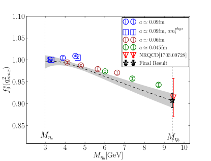
Figure 4: $f_{0}^{s}(q^{2}_{\text{max}})$ against $M_{\eta_{h}}$ (a proxy for the heavy quark mass). The grey band shows the result of our fit at $a=0$ and physical $l$, $s$ and $c$ masses. Notice that the $y$-axis scale does not begin at zero. We also include the result from a previous lattice calculation, which used the NRQCD discretisation for the $b$ quark with a non-relativistic expansion of the current through $\mathcal{O}(\Lambda/m_{b})$ and $\mathcal{O}(\alpha_{s})$ matching to continuum QCD Monahan et al. (2017). Sets of gluon field configurations listed in the legend follow the order of sets in table 1.

Source	% Fractional Error
Statistics	1.11
$m_{h}\to m_{b}$ and $a\to 0$	1.20
Quark mistuning	0.58
Total	1.73

Table 6: Error budget for $f_{0}^{s}(q^{2}_{\text{max}})$.

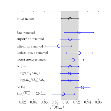
Figure 5: Results of tests of the $f_{0}^{s}(q^{2}_{\text{max}})$ fit. The top three blue points show $f_{0}^{s}(q^{2}_{\text{max}})$ at continuum and physical $b$ mass, if data from the fine, superfine or ultrafine ensembles are not used in the fit. The fourth and fifth blue points show the result if data at the highest/lowest $am_{h0}^{\text{val}}$ value on each ensemble are removed. The point labelled $N_{fit}=3$ is the result of extending the sum in Equation (29) so that it truncates at 3 rather than 2 in each of the $i,j,k$ directions. The points labelled $+\text{log}^{2}(M_{\eta_{h}}/M_{\eta_{c}})$ represents the result of adding a $\rho_{2}\text{log}^{2}(M_{\eta_{h}}/M_{\eta_{c}})$ term in the first set of brackets in Equation (29), where $\rho_{2}$ is a new fit parameter with the same prior distribution as $\rho$. Similarly for the $+\text{log}(M_{\eta_{h}}/M_{\eta_{c}})/M_{\eta_{h}}$ point. The point labelled ”no log” results from omitting the factor $(1+\rho\text{log}(M_{\eta_{c}}/M_{\eta_{h}}))$. The lowest point shows the value from the fit result for $R_{0}^{s}(q^{2}_{\text{max}})$, multiplied by the experimental value for $\sqrt{M_{B_{c}}}$ Tanabashi et al. (2018) and the result of our determination of $f_{B_{c}}$ at the physical point detailed in Appendix A of McLean et al. (2019).

III Results and Discussion

In tables 3 and 4, we give our results for the form factors on each ensemble along with the meson masses needed for the fits of the form factors as a function of $m_{h}$ and $a$ discussed in Section II.5.

We first show results from simplified fits to zero recoil data to find $f_{0,+}^{s}(q^{2}_{\text{max}})$. This allows us to test the behaviour in $m_{h}$. We then perform the larger fit, described in Section II.5, taking into account all the lattice data throughout the $q^{2}$ range.

III.0.1 Zero Recoil

We performed a fit to $f^{s}_{0}(q^{2}_{\text{max}})$ as a function of $m_{h}$ and $a$ using the fit form

$$f_{0}^{s}(q^{2}_{\text{max}})|_{\text{fit}}= \,\,\left(1+\rho\text{log}\left(M_{\eta_{h}}\over M_{\eta_{c}}\right)\right)\times$$

$$\sum_{i,j,k=0}^{2,2,2}d_{ijk}\left({2\Lambda_{\text{QCD}}\over M_{\eta_{h}}}\right)^{i}\left({am^{\text{val}}_{h0}\over\pi}\right)^{2j}\left({am^{\text{val}}_{c0}\over\pi}\right)^{2k}$$

$$\times\left(\,1+\mathcal{N}_{\text{mistuning}}\,\right)\,.$$ (33)

This is the same fit function as described earlier for the individual $z$-space coefficients in Equation (29) and we take the same priors for the corresponding coefficients as discussed there.

The fit has $\chi^{2}/N_{\text{dof}}=0.21$, for 12 degrees of freedom. Evaluating the result at $a=0$ and physical $b$ quark mass, we find

$$f_{0}^{s}(q^{2}_{\text{max}})=0.907(16)\,.$$ (34)

We show the dependence on $M_{\eta_{h}}$ of our results and the fit in Figure 4. The error budget corresponding to Equation (34) is given in Table 6. Note that we do not impose the constraint that $f_{0}^{s}(q^{2}_{\text{max}})=1.0$ when $m_{h}=m_{c}$. If we do this, we reduce the uncertainty in Equation (34) by 25%.

We include in Figure 4 a previous lattice determination of $f_{0}^{s}(q^{2}_{\text{max}})$ Monahan et al. (2017), shown as a red triangle. Our result, containing independent uncertainties, is in agreement with this earlier value but much more accurate. The older study used the $n_{f}=2+1$ MILC asqtad gluon ensembles, with HISQ $s$ and $c$ valence quarks, and an NRQCD $b$ quark. Using NRQCD meant that the calculation could be performed directly at the physical $b$ mass. However, the matching of lattice NRQCD currents to continuum QCD, performed at $\mathcal{O}(\alpha_{s})$, is a significant source of systematic error absent in our calculation.

We perform a number of tests of the fit at zero recoil, and present results in Figure 5. The tests show that the fits are robust.

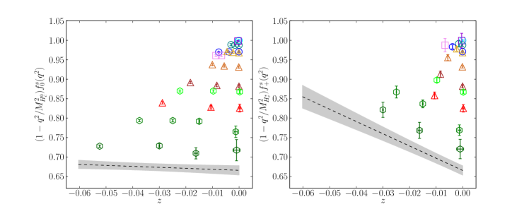
Figure 6: $Pf_{0,+}^{s}$ in $z$-space, where $P$ is the appropriate pole function for each form factor given in Equation (27). The grey band shows the result of our fit at $a=0$ and physical $l$,$s$, $c$ and $b$ masses. Sets listed in the legend follow the order of sets in Table 1.

III.0.2 Full $q^{2}$ range

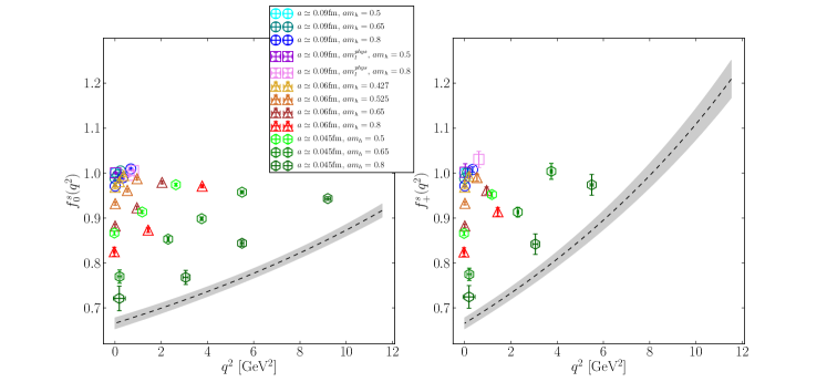
Figure 7: $f_{0,+}^{s}(q^{2})$ against $q^{2}$. The grey band shows the result of our fit at $a=0$ and physical $l$,$s$, $c$ and $b$ masses. Sets listed in the legend follow the order of sets in Table 1.

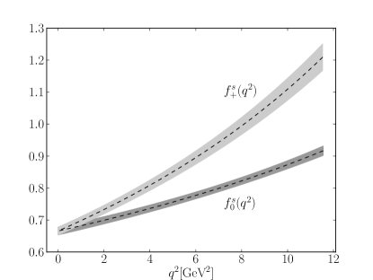
Figure 8: Final result for $f_{0,+}^{s}(q^{2})$ against $q^{2}$ at the physical point .

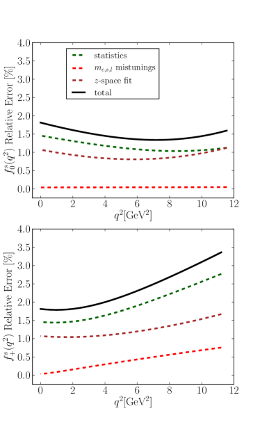
Figure 9: Error budget for $f_{0,+}^{s}(q^{2})$ as a function of $q^{2}$ .

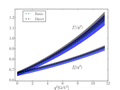
Figure 10: Results for $f_{0,+}^{s}(q^{2})$ against $q^{2}$ at the physical point, comparing the ratio method (from Appendix B) and the direct method (from Section III.0.2).

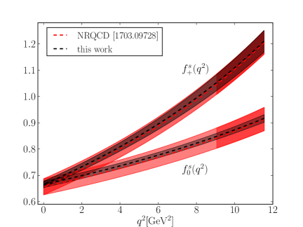
Figure 11: Our final result for $f_{0,+}^{s}(q^{2})$ compared to form factors calculated using an NRQCD action for the $b$ quark Monahan et al. (2017). Part of the NRQCD band is shaded darker than the rest ($q^{2}\gtrapprox 9.5$GeV²) to signify the region where lattice results were directly calculated. The NRQCD form factors in the rest of the $q^{2}$ range are the result of an extrapolation using a BCL parameterization.

We now proceed to fit our full set of data including zero and non-zero recoil points to the fit form given in Equations (27) and (29) and discussed in Section II.5. We include the covariance matrix between the form factor values obtained from correlator fits on a given ensemble along with correlated lattice spacing uncertainties. The goodness of fit obtained is $\chi^{2}/N_{\text{dof}}=0.51$, with 58 degrees of freedom.

In Figure 6 we show our results and fit function in $z$-space for the form factors multiplied by their appropriate pole factors, $P$, given by $1-q^{2}/M_{H_{c}^{0,*}}$ in Equation (27). This shows that the $z$-dependence is relatively benign for both form factors and the main $m_{h}$-dependent effect is the smooth reduction in value of $Pf$ as $m_{h}$ increases. The final result at the physical $b$ quark mass is given by the grey band.

In Figure 7, we show the results and fit function in $q^{2}$-space. The form factors for the physical $b$ quark mass (i.e. those corresponding to $B_{s}\to D_{s}$ decay) are given by the grey band.

Figure 8 shows the physical $f_{+}$ and $f_{0}$ form factors on the same plot and covering the full $q^{2}$ range for the $B_{s}\to D_{s}$ decay. Figure 9 plots the associated error budget for the two form factors throughout the $q^{2}$ range. The dominant uncertainty comes from statistical errors. There are also significant uncertainties from the $q^{2}$ and $m_{h}$ dependence for $f_{+}$ at larger values of $q^{2}$. This is because there are no lattice QCD results at $q^{2}_{\text{max}}$ for $f_{+}$. The impact of uncertainties in the lattice spacing (both in $w_{0}/a$ and in $w_{0}$) are smaller than the errors shown in the Figure and so not plotted there. This is because the form factors themselves are dimensionless and lattice spacing effects in the determination of $q^{2}$ largely cancel as, for example, the pole masses are given in terms of lattice masses.

As discussed in Section II.5 an alternative approach to the fit is to take ratios of the form factors to the $H_{c}$ decay constant and fit the ratios to the fit form of Eqs. (27) and (29). This fit is described in Appendix B. It has the advantage of smaller discretisation effects but the disadvantage of larger lattice spacing uncertainties because the ratios being fit are dimensionful. In the end the ratio method has larger uncertainty for the final physical form factors. We therefore take the results from the direct method as our final result, and use the ratio method results as a consistency test. Since the two approaches have quite different systematic errors, their comparison supplies a strong consistency check. In Figure 10, we plot the form factors from the two methods on top of each other. As is clear from this plot, the results are in good agreement. The direct method gives a more accurate result for both form factors and at all $q^{2}$.

We compare the coefficients from our fits to unitarity bounds in Appendix C as a further test.

In Figure 11, we compare our final form factors to those determined from the lattice QCD calculation using the NRQCD approach for the $b$ quark already used as a comparison at $q^{2}_{\text{max}}$ in Figure 4 Monahan et al. (2017). The NRQCD calculation works directly at the $b$ quark mass but on relatively coarse lattices and hence is unable to obtain results at large physical momenta for the $D_{s}$ meson. The results close to zero-recoil are extrapolated to $q^{2}=0$ using a $z$-space parameterisation. As the Figure shows, our results are in excellent agreement with the NRQCD calculation but are more precise for both $f^{s}_{0}(q^{2})$ and $f^{s}_{+}(q^{2})$ throughout all $q^{2}$. This is because we can avoid the significant systematic uncertainty that the NRQCD calculation has from the perturbative matching to continuum QCD of the NRQCD current that couples to the $W$.

III.1 $R({D_{s}})$

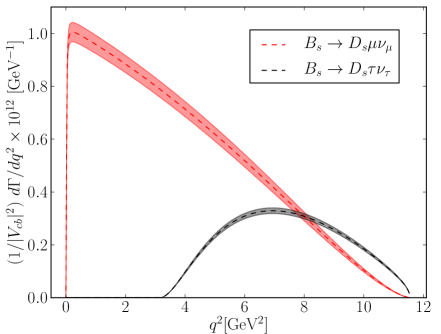
Figure 12: Differential decay rates for the $B_{s}\to D_{s}\mu\nu_{\mu}$ and $B_{s}\to D_{s}\tau\nu_{\tau}$ decays, calculated using the form factors determined in this work.

Source	% Fractional Error
Statistics	1.11
$z$-space fit	1.05
Quark Mass Mistuning	0.12
Total	1.54

Table 7: Error budget for our result for $R({D_{s}})$ in the SM. $z$-space fit refers to the error associated with the fit of the dependence on heavy quark mass and lattice spacing and interpolation in $q^{2}$.

Using our calculated form factors $f^{s}_{0,+}(q^{2})$, we can calculate the differential rate for $B_{s}\to D_{s}\ell\nu$ decay from Equation (1). This is a function of the lepton mass and so differs between the heavy $\tau$ and the light $e$, $\mu$ leptons. The differential rate for $\mu$ and $\tau$ is compared in Figure 12. We take the meson and lepton masses needed for Equation (1) from Tanabashi et al. (2018) and $\eta_{\text{EW}}$ = 1.011(5) Na et al. (2015). The distribution in the $\tau$ case is cut off at $q^{2}=m_{\tau}^{2}$ and so, although there is enhancement from $m_{\ell}^{2}/q^{2}$ terms in Equation (1) that reflect reduced helicity suppression, the integrated branching fraction for the $\tau$ case is smaller than for the $\mu$.

The ratio of branching fractions for semileptonic $B$ decays to $\tau$ and to $e$/$\mu$ is being used as a probe of lepton universality with an interesting picture emerging Amhis et al. (2017); Caria (2019). Here we provide a new SM prediction for the quantity

$$R({D_{s}})={\mathcal{B}(B_{s}\to D_{s}\tau\nu_{\tau})\over\mathcal{B}(B_{s}\to D_{s}l\nu_{l})}\,,$$ (35)

where $l=e$ or $\mu$ (the difference between $e$ and $\mu$ is negligible in comparison to our precision on $R(D_{s})$). Our result is

$$\left.R(D_{s})\right|_{\text{SM}}=0.2987(46),$$ (36)

in which we averaged over the $l=e$ and $l=\mu$ cases. Note that $|V_{cb}|$ and $\eta_{\text{EW}}$ cancel in this ratio. We give an error budget for this result in terms of the uncertainties from our lattice QCD calculation in Table 7. Our result agrees with, but is more accurate than, the previous lattice QCD value of $R(D_{s})$ (0.301(6)) from Monahan et al. (2017). An experimental result for $R(D_{s})$ would allow a new test of lepton universality.

We expect very little difference between $R(D_{s})$ and the analogous quantity $R(D)$ because the mass of the spectator quark has little effect on the form factors Bailey et al. (2012). Lattice QCD calculations that involve light spectator quarks have larger statistical errors, however, which is why the process $B_{s}\to D_{s}$ is under better control. Previous lattice QCD results for $R(D)$ are 0.300(8) Na et al. (2015) and 0.299(11) Bailey et al. (2015), in which any difference with our result for $R(D_{s})$ is too small to be visible with these uncertainties.

IV Comparison to HQET

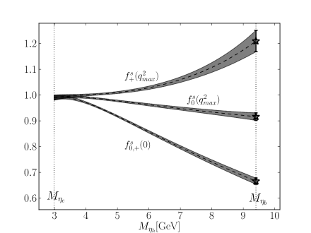
Figure 13: Form factor values at $q^{2}_{\text{max}}$ and $q^{2}=0$ plotted against $M_{\eta_{h}}$, a proxy for the heavy quark mass.

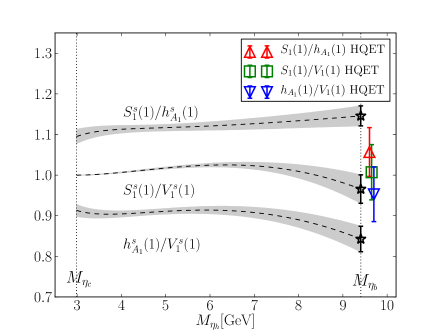
Figure 14: Form factor ratios against $M_{\eta_{h}}$, a proxy for the heavy quark mass. $S_{1}^{s}$ and $V_{1}^{s}$ are defined in Eqs. (38) and (39). Note that only two of these ratios are independent. The colourful points are NLO HQET expectations from Bernlochner et al. (2017), derived with input from QCD sum rules. The HQET error bars each include a 6% uncertainty to allow for missing higher-order terms.

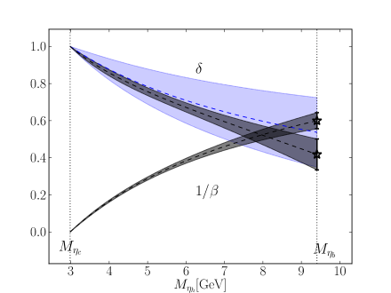
Figure 15: We show two quantities derived from the form factor slopes as a function of $M_{\eta_{h}}$. $1/\beta(m_{h})$ is defined in Equation (43)) and $\delta$ in Equation (44). Our results are shown by the grey bands. The blue band shows the leading order HQET expectation for $\delta$ given in Equation (46).

In Figure 13 we show our form factor results at two key values of $q^{2}$, the zero recoil point and $q^{2}=0$, as a function of heavy quark mass, given by $M_{\eta_{h}}$. The plot demonstrates how $f_{+}$ at zero-recoil increases as the heavy quark mass increases, but $f_{0}$ changes very little. The value at $q^{2}=0$, where the form factors are equal, falls with growing heavy quark mass, as the $q^{2}$ range opens up.

Knowledge of the functional form of $f_{0}^{s}(q^{2})$ and $f_{+}^{s}(q^{2})$, along with that of the $B_{s}\rightarrow D_{s}^{*}\ell\nu$ form factor at zero recoil, $h_{A_{1}}^{s}(1)$, from McLean et al. (2019), against $m_{h}$ gives us access to the functional form in $m_{h}$ of a number of quantities of interest in HQET.

In HQET the vector current matrix element is parameterized with a different set of form factors, $h^{s}_{+}(w)$ and $h^{s}_{-}(w)$ according to

$${\langle D_{s}|V^{\mu}|H_{s}\rangle\over\sqrt{M_{D_{s}}M_{H_{s}}}}=h^{s}_{+}(w)(v+v^{\prime})^{\mu}+h^{s}_{-}(w)(v-v^{\prime})^{\mu}\,,$$ (37)

where $v^{\mu}=p_{H_{s}}^{\mu}/M_{H_{s}}$ and $v^{\prime\mu}=p_{D_{s}}^{\mu}/M_{D_{s}}$ are the 4-velocities of the initial and final state mesons, and $w=v\cdot v^{\prime}$ is an alternative parameter to $q^{2}$ used in the context of HQET.

As a test of HQET, one can construct ratios of form factors that should become unity in the $m_{c},m_{h}\to\infty$ limit. Following Caprini et al. (1998), one can redefine the form factors such that each of them reduce to the Isgur-Wise function $\xi(w)$ in the $m_{c},m_{h}\to\infty$ limit. In the $B_{s}\to D_{s}$ case these new form factors are

$$S^{s}_{1}(w) =h^{s}_{+}(w)-{1+r\over 1-r}{w-1\over w+1}h^{s}_{-}(w)\,,$$ (38)

$$V^{s}_{1}(w) =h^{s}_{+}(w)-{1-r\over 1+r}h^{s}_{-}(w)\,,$$ (39)

where $r=M_{D_{s}}/M_{H_{s}}$. $h_{A_{1}}^{s}$ also reduces to $\xi$ in the infinite mass limit. Hence any ratio between $S^{s}_{1}$,$V^{s}_{1}$ and $h_{A_{1}}^{s}$ should become unity in this limit. From our results at zero recoil and for $m_{h}=m_{b}$ we find

$${S^{s}_{1}(1)\over h^{s}_{A_{1}}(1)}\bigg{|}_{\text{lat}} =1.146(25)$$ (40)

$${S^{s}_{1}(1)\over V^{s}_{1}(1)}\bigg{|}_{\text{lat}} =0.966(35)$$ (41)

$${h^{s}_{A_{1}}(1)\over V^{s}_{1}(1)}\bigg{|}_{\text{lat}} =0.843(31)$$ (42)

Fig. 14 illustrates how these ratios vary with $m_{h}$, and gives the NLO HQET expectation for these values for comparison Bernlochner et al. (2017). The HQET results include a 6% uncertainty to allow for missing higher order terms in $\alpha_{s}^{2}$, $\alpha_{s}\overline{\Lambda}/m_{c}$ and $(\overline{\Lambda}/m_{c})^{2}$ as suggested for these ratios in Bigi et al. (2017b). Our results show some tension with the HQET expectations that might indicate that the missing higher order contributions are bigger than 6%. This is discussed in Bigi et al. (2017b) in the context of earlier lattice QCD results. Preliminary results from the JLQCD collaboration Kaneko et al. (2018) show similar values to ours.

Another set of quantities of interest in HQET are the slopes of the form factors at $q^{2}=0$ Hill (2006a, b):

$${1\over\beta(m_{h})}\equiv \,\,{M_{H_{s}}^{2}-M_{D_{s}}^{2}\over f^{s}_{+}(0)}\,{df^{s}_{+}\over dq^{2}}\bigg{|}_{q^{2}=0}\,,$$ (43)

$$\delta(m_{h})\equiv \,\,1-{M_{H_{s}}^{2}-M_{D_{s}}^{2}\over f^{s}_{+}(0)}\left({df^{s}_{+}\over dq^{2}}\bigg{|}_{q^{2}=0}-{df^{s}_{0}\over dq^{2}}\bigg{|}_{q^{2}=0}\right)\,.$$ (44)

To obtain these values from our results for the form factors, we take the derivative of the fit function (Equation (29)) evaluated at continuum and physical $l,s$ and $c$ masses. At $m_{h}=m_{b}$ we find

$${1\over\beta(m_{b})}=0.600(43)\,,\quad\delta(m_{b})=0.405(84)\,.$$ (45)

In Figure 15 we show how these quantities vary with $m_{h}$. By rewriting Equation (44) in terms of $h^{s}_{+,-}$, and recognising that in the heavy quark limit $h^{s}_{+}\approx\xi$ and $h^{s}_{-}\approx 0$, one can find a leading order HQET expectation for $\delta$ Hill (2006b):

$$\delta(m_{h}) ={2M_{D_{s}}\over M_{H_{s}}+M_{D_{s}}}{1+{h_{-}\over h_{+}}\over 1-{M_{H_{s}}-M_{D_{s}}\over M_{H_{s}}+M_{D_{s}}}{h_{-}\over h_{+}}}$$ (46)

$$={2M_{D_{s}}\over M_{H_{s}}+M_{D_{s}}}\left[1+\right.$$

$$\left.\left(\frac{M_{H_{s}}-M_{D_{s}}}{M_{H_{s}}+M_{D_{s}}}\right)\mathcal{O}(\alpha_{s},\Lambda_{\text{QCD}}/m_{h},\Lambda_{\text{QCD}}/m_{c})\right]\,.$$

This leading order expression, along with an uncertainty from missing higher-orders as indicated above, is shown in Figure 15 as a blue band. Note that by definition $\delta(m_{c})=1$. Our results (grey band) are in good agreement with this, up to the uncertainties from higher order terms shown in Equation (46).

V Conclusions

We have calculated the scalar and vector form factors for the $B_{s}\to D_{s}\ell\nu$ decay for the full $q^{2}$ range using lattice QCD with a fully nonperturbative normalisation of the current operators for the first time. Our calculation used correlation functions at three values of the lattice spacing, including an ensemble with an approximately physical light quark mass. We used the relativistic HISQ action with a range of values for the heavy valence quark and by fitting this dependence, along with the lattice spacing dependence, we are able to determine results at the $b$ quark mass. The valence $c$ and $s$ quark masses are accurately tuned to their physical values. By working on very fine lattices we are able both to reach a heavy quark mass close to the $b$ but also to cover the full $q^{2}$ range of the decay.

Our results for the form factors are given in Figure 8 and the differential rate that this implies for $B_{s}\to D_{s}\ell\nu$ in Figure 12. This will allow a determination of $|V_{cb}|$ from future experimental data from this semileptonic process. Instructions on how to reproduce our form factors are given in Appendix A. Our error budget is given in Figure 9.

Our results are more accurate than previous lattice QCD determinations using a nonrelativistic $b$ quark formalism because we do not have a systematic uncertainty from the perturbative matching of the lattice current to continuum QCD.

From our results we can predict the ratio $R(D_{s})$ of the branching fraction to a $\tau$ lepton compared to that to $e$/$\mu$ (see Section III.1). We are also able to compare functions of the form factors and their slopes to HQET expectations (see Section IV).

Our calculation shows that a heavy-HISQ determination of the $B\to D\ell\nu$ form factors is feasible. This would allow direct comparison to existing experimental data. Such a calculation could use an identical strategy to the one demonstrated here, with the strange valence quark replaced with a light one and additional calculations on ensembles spanning a range of light quark masses. Higher statistics would be needed since statistical uncertainties will be larger than in this calculation, and the issue of topology freezing on fine lattices will be more significant. Our calculation demonstrates, however, that lattice QCD is no longer limited for these form factors by the systematic uncertainties coming from current matching and, with sufficient computer time, a  1% accurate result for $B\to D\ell\nu$ form factors is achieveable.

Acknowledgements

We are grateful to the MILC collaboration for the use of their configurations and their code. Computing was done on the Cambridge Service for Data Driven Discovery (CSD3) supercomputer, part of which is operated by the University of Cambridge Research Computing Service on behalf of the UK Science and Technology Facilities Council (STFC) DiRAC HPC Facility. The DiRAC component of CSD3 was funded by BEIS via STFC capital grants and is operated by STFC operations grants. We are grateful to the CSD3 support staff for assistance. Funding for this work came from STFC. We would also like to thank C. Bouchard, B. Colquhoun, D. Hatton, J. Harrison, P. Lepage, Z. Ligeti and M. Wingate for useful discussions

Appendix A Reconstructing Form Factors

This appendix gives the necessary information to reproduce the functional form of the form factors through $q^{2}$ reproduced in this work. We here express the form factors in terms of the BCL parameterisation Bourrely et al. (2009):

$$f^{s}_{0}(q^{2})={1\over 1-{q^{2}\over M_{B_{c0}}^{2}}}\sum_{n=0}^{2}a_{n}^{0}z^{n}(q^{2}),$$ (47)

$$f^{s}_{+}(q^{2})={1\over 1-{q^{2}\over M_{B_{c}^{*}}^{2}}}\sum_{n=0}^{2}a_{n}^{+}\left(z^{n}(q^{2})-{n\over 3}(-1)^{n-3}z^{3}(q^{2})\right),$$

where the function $z(q^{2})$ is defined by defined by

$$z(q^{2})={\sqrt{t_{+}-q^{2}}-\sqrt{t_{+}}\over\sqrt{t_{+}-q^{2}}+\sqrt{t_{+}}},$$ (48)

and $t_{+}=(M_{B_{s}}+M_{D_{s}})^{2}$. We take the PDG 2018 values for these masses, 5.3669 GeV for the $B_{s}$ and 1.9683 GeV for the $D_{s}$ Tanabashi et al. (2018). For the position of the poles, we use $M_{B_{c0}}=6.704$GeV and $M_{B_{c}^{*}}=6.329$GeV. The coefficients $a_{n}^{0,+}$ found from our fit, along with their covariance, is given in Table 8. The form factor values at the two ends of the $q^{2}$ range are: $f^{s}_{+}(q^{2}_{\text{max}})=1.209(42)$; $f^{s}_{0}(q^{2}_{\text{max}})=0.917(15)$ (note that this value differs slightly from that in Eq. (34) because this value comes from a fit that includes all $q^{2}$ values); $f^{s}_{+}(q^{2}=0)=f_{0}(q^{2}=0)=0.666(12)$.

	$a^{0}_{0}$	$a^{0}_{1}$	$a^{0}_{2}$	$a^{+}_{0}$	$a^{+}_{1}$	$a^{+}_{2}$
	0.66574	-0.25944	-0.10636	0.66574	-3.23599	-0.07478
	0.00015	0.00188	0.00070	0.00015	0.00022	0.00003
		0.06129	0.16556	0.00188	0.01449	0.00001
			3.29493	0.00070	0.18757	-0.00614
				0.00015	0.00022	0.00003
					0.20443	0.10080
						4.04413

Table 8: Our results for $z$-coefficients in the BCL parameterization Equation (47). The first row gives mean values, and the rest of the table gives the covarance matrix associated with these parameters.

Appendix B The ratio method for obtaining the form factors

Here we show results from the ratio approach to determining the form factors. In this approach we fit the ratio of the form factors to decay constant of the pseudoscalar $H_{c}$ meson McLean et al. (2019):

$$R^{s}_{0,+}(q^{2})\equiv{f^{s}_{0,+}(q^{2})\over f_{H_{c}}\sqrt{M_{H_{c}}}}.$$ (49)

Two-point correlation functions for the $H_{c}$ meson are calculated along with the other two- and three-point correlation functions that we need (see Section II.2) and included in the simultaneous fits to these correlation functions described in Section II.3. This enables us to determine the heavy-charm meson decay constant (and in fact the combination $f_{H_{c}}\sqrt{M_{H_{c}}}$ needed for Equation (49)) from the amplitude for the ground-state in the two-point correlation functions as given in Equation (22). Our results for $R^{s}_{0,+}(q^{2})$ are given in Table 4.

We fit $R^{s}_{0,+}(q^{2})$ using an identical fit function to that of the direct approach, given in Equations (27) and (29).

Discretisation effects change in the ratio given in Equation (49), compared to those from the form factors themselves, changing the continuum extrapolation. The dependence on heavy quark mass of the ratio is also very different. The value of the ratio at the physical point (where $m_{h}=m_{b}$ and $a=0$) can then multiplied by $f_{B_{c}}\sqrt{M_{B_{c}}}$ to obtain the form factors. We find $f_{B_{c}}$ via a separate calculation (detailed in Appendix A of McLean et al. (2019)) and take the experimental value for the $B_{c}$ meson mass, $M_{B_{c}}=6.2756(11)$GeV Tanabashi et al. (2018). This approach has the disadvantage of introducing larger uncertainties from scale-setting since $R_{0,+}^{s}(q^{2})$ are dimensionful quantities (as opposed to $f^{s}_{0,+}(q^{2})$ which are dimensionless). Hence we do not use it for our final value. It provides a useful test of our uncertainties, however.

Figure 16: $R_{0}^{s}(q^{2}_{\text{max}})=f_{0}^{s}(q^{2}_{\text{max}})/(f_{H_{c}}\sqrt{M_{H_{c}}})$ against $M_{\eta_{h}}$ (a proxy for the heavy quark mass). The grey band shows the result of the extrapolation at $a=0$ and physical $l$,$s$ and $c$ masses. Sets listed in the legend follow the order of sets in table 1.

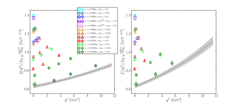
Figure 17: $R_{0,+}^{s}(q^{2})=f_{0,+}^{s}(q^{2})/(f_{H_{c}}\sqrt{M_{H_{c}}})$ against $q^{2}$. The grey band shows the result of our fit at $a=0$ and physical $l$,$s$, $c$ and $b$ masses. Sets listed in the legend follow the order of sets in table 1.

B.0.1 Zero Recoil

Source	% Fractional Error
Statistics	1.10
Scale Setting	1.30
$m_{h}\to m_{b}$ and $a\to 0$	1.44
Quark mistuning	0.87
Total	2.39

Table 9: Error budget for $R_{0}^{s}(q^{2}_{\text{max}})$.

We first show results from a fit at the zero recoil point, $R^{s}_{0}(q^{2}_{\text{max}})$, as a function of heavy quark mass and lattice spacing. To do this we use the same fit form as for our fits to $f^{s}_{0,+}(q^{2}_{\text{max}})$, given in Equation (33), with the same priors. We find, with physical parameters for all quark masses and $a=0$

$$R_{0}^{s}(q^{2}_{\text{max}})={f_{0}^{s}(q^{2}_{\text{max}})\over f_{B_{c}}\sqrt{M_{B_{c}}}}=0.853(20)\text{GeV}^{-3/2}\,.$$ (50)

The fit has $\chi^{2}/N_{\text{dof}}=0.63$ for $N_{\text{dof}}=16$. The lattice QCD results and fit are shown in a plot against $M_{\eta_{h}}$ in Figure 16. As can be seen from this plot, the lattice results have stronger dependence on the heavy quark mass and somewhat less on the lattice spacing compared to that seen in Figure 4. The error budget for our physical value in Equation (50) is given in Table 9. Notice that, compared to Table 6 it now has a significant scale-setting uncertainty.

B.0.2 Full $q^{2}$ range

In Figure 17, we show the complete set of lattice results along with the results of the full fit given by the fit form in Equation (29). As for Figure 7 we see that as the lattice spacing decreases, the range of heavy quark masses increases and the $q^{2}$ range, $0<(M_{H_{s}}-M_{D_{s}})^{2}$ expands. The goodness of fit here was $\chi^{2}/N_{\text{dof}}=0.57$, $N_{\text{dof}}=58$.

To obtain the form factors, the resulting functions $R_{0,+}^{s}(q^{2})$ were multiplied by $\sqrt{M_{B_{c}}}$ (using the experimental value) and $f_{B_{c}}$ from our determination detailed in appendix A of McLean et al. (2019). The resulting form factors are shown in Figure 10 in a comparison to those found by our direct method of Section III.0.2.

Appendix C Tests of Unitarity Bounds

Unitarity and crossing symmetry imposes bounds on the coefficients of the BCL parameterization of $f_{0,+}(q^{2})$, $\{a_{n}\}$ Okubo (1971a, b). As another consistency test, we show here that the coefficients found in our fit satisfy these bounds.

To obtain bounds on the BCL coefficients Bourrely et al. (2009), one must relate them to those of a different parameterisation, that of Boyd, Grinstein and Lebed (BGL) Boyd et al. (1996):

$$f_{0,+}^{s}(q^{2})={1\over B(z)\phi(z)}\sum^{N}_{n\geq 0}b_{n}z^{n}.$$ (51)

$B(z)$ is known as the Blashke factor:

$$B(z)={z-z_{*}\over 1-zz_{*}}\,,$$ (52)

where $z_{*}=z(M^{2}_{B_{c}^{0}})$ for $f_{0}^{s}$, or $z(M^{2}_{B_{c}^{*}})$ for $f_{+}^{s}\,$. $\phi(z)$ is the outer function;

$$\phi(z) =M_{B_{s}}^{2-s}2^{2+p}\sqrt{\kappa n_{f}}\left[{M_{D_{s}}\over M_{B_{s}}}(1+z)\right]^{s-3/2}$$

$$\times \left[(1-z)\left(1+{M_{D_{s}}\over M_{B_{s}}}\right)+2\sqrt{M_{D_{s}}\over M_{B_{s}}}(1+z)\right]^{-s-p}.$$ (53)

In the $f^{s}_{0}$ case, $\kappa=12\pi M^{2}_{B_{s}}\chi_{A}$, $p=1$, $s=3$. In the $f^{s}_{+}$ case, $\kappa=6\pi M^{2}_{B_{s}}\chi_{V}$, $p=3$, $s=2$. The quantities $\chi_{V,A}$ are the once-subtracted dispersion relations at $q^{2}=0$ for vector and axial $b\to c$ currents respectively, computed in Boyd et al. (1996) to be $\chi_{V}=5.7\times 10^{-3}/m_{b}^{2}$ and $\chi_{A}=9.6\times 10^{-3}/m_{b}^{2}$.

The BGL coefficients, $\{b_{n}\}$, obey the unitarity constaint

$$\sum_{m=0}^{\infty}|b_{m}|^{2}\leq 1$$ (54)

by construction of the parameterisation. To see how this applies to the BCL coefficients $\{a_{n}\}$, one must relate them to $\{b_{m}\}$ by equating the two parameterisations to find Bourrely et al. (2009)

$$\sum^{M}_{m=0}b_{m}z^{m}=\psi(z)\sum_{n=0}^{N}a_{n}z^{n},$$ (55)

where $\psi(z)$ is given by

$$\psi(z)={M_{\text{pole}}^{2}\over 4(t_{+}-t_{0})}\phi(z){(1-z)^{2}(1-z_{*})^{2}\over(1-zz_{*})^{2}},$$ (56)

and $M_{\text{pole}}=M_{B_{c}^{0}}$ in the $f^{s}_{0}$ case and $M_{B_{c}^{*}}$ in the $f^{s}_{+}$ case. Expanding $\psi(z)$ around $z=0$, comparing coefficients of $z$ in Equation (55), and imposing the constraint of Equation (54), we arrive at a constraint for the BCL coefficients

$$\mathcal{B}\equiv\sum_{j,k=0}^{L,L}B_{jk}a_{j}a_{k}\leq 1\,,$$ (57)

$$B_{jk}=\sum_{n=0}^{\infty}\eta_{n}\eta_{n+|j-k|}\,,$$ (58)

where $\{\eta_{n}\}$ are the Taylor coefficients of $\psi(z)$.

	$B_{00}$	$B_{01}$	$B_{02}$
$f^{s}_{0}$	0.00186	-0.000258	-0.000703
$f^{s}_{+}$	0.00179	-0.000367	0.00108

Table 10: Numerical values for $B_{jk}$ appearing in the unitarity bound for BCL coefficients, defined in (58), for the $f^{s}_{0}$ and $f^{s}_{+}$ cases. The rest of the elements can be obtained from these using the properties $B_{j(j+k)}=B_{0k}$ and $B_{jk}=B_{kj}$.

$\psi(z)$ is bounded on the closed disk $|z|<1$, so its Taylor coefficients are rapidly decreasing. We computed values for $B_{jk}$ by truncating the sum in its definition (Equation (58)) at 100. These values are given in Table 10. With these $B_{jk}$ values, and the $a_{n}$ coefficients from our fit (via the direct method), we find

$$\mathcal{B}_{0}=0.00073(89)\,,$$

$$\mathcal{B}_{+}=0.0210(54)\,.$$

These comfortably satisfy the unitarity bound. Additionally, as discussed in Becher and Hill (2006), the leading contributions to $\mathcal{B}_{0,+}$ are of order $(\Lambda_{\text{QCD}}/m_{b})^{3}\simeq 10^{-3}$ in the heavy quark expansion. This expectation is approximately fulfilled by our result.

References

- Wei et al. (2009) J. T. Wei et al. (Belle), Phys. Rev. Lett. 103, 171801 (2009), arXiv:0904.0770 [hep-ex] .
- Lees et al. (2012a) J. P. Lees et al. (BaBar), Phys. Rev. Lett. 109, 101802 (2012a), arXiv:1205.5442 [hep-ex] .
- Lees et al. (2012b) J. P. Lees et al. (BaBar), Phys. Rev. D86, 032012 (2012b), arXiv:1204.3933 [hep-ex] .
- Lees et al. (2013) J. P. Lees et al. (BaBar), Phys. Rev. D88, 072012 (2013), arXiv:1303.0571 [hep-ex] .
- Aaij et al. (2014a) R. Aaij et al. (LHCb), JHEP 06, 133 (2014a), arXiv:1403.8044 [hep-ex] .
- Aaij et al. (2014b) R. Aaij et al. (LHCb), Phys. Rev. Lett. 113, 151601 (2014b), arXiv:1406.6482 [hep-ex] .
- Huschle et al. (2015) M. Huschle et al. (Belle), Phys. Rev. D92, 072014 (2015), arXiv:1507.03233 [hep-ex] .
- Aaij et al. (2016a) R. Aaij et al. (LHCb), JHEP 02, 104 (2016a), arXiv:1512.04442 [hep-ex] .
- Aaij et al. (2015a) R. Aaij et al. (LHCb), Phys. Rev. Lett. 115, 111803 (2015a), [Erratum: Phys. Rev. Lett.115,159901(2015)], arXiv:1506.08614 [hep-ex] .
- Aaij et al. (2015b) R. Aaij et al. (LHCb), JHEP 06, 115 (2015b), [Erratum: JHEP09,145(2018)], arXiv:1503.07138 [hep-ex] .
- Aaij et al. (2016b) R. Aaij et al. (LHCb), JHEP 11, 047 (2016b), [Erratum: JHEP04,142(2017)], arXiv:1606.04731 [hep-ex] .
- Wehle et al. (2017) S. Wehle et al. (Belle), Phys. Rev. Lett. 118, 111801 (2017), arXiv:1612.05014 [hep-ex] .
- Sato et al. (2016) Y. Sato et al. (Belle), Phys. Rev. D94, 072007 (2016), arXiv:1607.07923 [hep-ex] .
- Hirose et al. (2018) S. Hirose et al. (Belle), Phys. Rev. D97, 012004 (2018), arXiv:1709.00129 [hep-ex] .
- Aaij et al. (2018a) R. Aaij et al. (LHCb), Phys. Rev. D97, 072013 (2018a), arXiv:1711.02505 [hep-ex] .
- Aaij et al. (2018b) R. Aaij et al. (LHCb), Phys. Rev. Lett. 120, 171802 (2018b), arXiv:1708.08856 [hep-ex] .
- Aaij et al. (2017) R. Aaij et al. (LHCb), JHEP 08, 055 (2017), arXiv:1705.05802 [hep-ex] .
- Sirunyan et al. (2018) A. M. Sirunyan et al. (CMS), Phys. Lett. B781, 517 (2018), arXiv:1710.02846 [hep-ex] .
- Aaboud et al. (2018) M. Aaboud et al. (ATLAS), JHEP 10, 047 (2018), arXiv:1805.04000 [hep-ex] .
- Aubert et al. (2009) B. Aubert et al. (BaBar), Phys. Rev. D79, 012002 (2009), arXiv:0809.0828 [hep-ex] .
- Aubert et al. (2010) B. Aubert et al. (BaBar), Phys. Rev. Lett. 104, 011802 (2010), arXiv:0904.4063 [hep-ex] .
- Bailey et al. (2015) J. A. Bailey et al. (MILC), Phys. Rev. D92, 034506 (2015), arXiv:1503.07237 [hep-lat] .
- Na et al. (2015) H. Na, C. M. Bouchard, G. P. Lepage, C. Monahan, and J. Shigemitsu (HPQCD), Phys. Rev. D92, 054510 (2015), [Erratum: Phys. Rev.D93,no.11,119906(2016)], arXiv:1505.03925 [hep-lat] .
- Glattauer et al. (2016) R. Glattauer et al. (Belle), Phys. Rev. D93, 032006 (2016), arXiv:1510.03657 [hep-ex] .
- Bernlochner et al. (2017) F. U. Bernlochner, Z. Ligeti, M. Papucci, and D. J. Robinson, Phys. Rev. D95, 115008 (2017), [Erratum: Phys. Rev.D97,no.5,059902(2018)], arXiv:1703.05330 [hep-ph] .
- Bigi et al. (2017a) D. Bigi, P. Gambino, and S. Schacht, Phys. Lett. B769, 441 (2017a), arXiv:1703.06124 [hep-ph] .
- Grinstein and Kobach (2017) B. Grinstein and A. Kobach, Phys. Lett. B771, 359 (2017), arXiv:1703.08170 [hep-ph] .
- Tanabashi et al. (2018) M. Tanabashi et al. (Particle Data Group), Phys. Rev. D98, 030001 (2018).
- Lees et al. (2019) J. P. Lees et al. (BaBar), (2019), arXiv:1903.10002 [hep-ex] .
- Gambino et al. (2019) P. Gambino, M. Jung, and S. Schacht, (2019), arXiv:1905.08209 [hep-ph] .
- Koponen et al. (2013) J. Koponen, C. T. H. Davies, G. C. Donald, E. Follana, G. P. Lepage, H. Na, and J. Shigemitsu (HPQCD), (2013), arXiv:1305.1462 [hep-lat] .
- McLean et al. (2018) E. McLean, C. T. H. Davies, A. T. Lytle, and J. Koponen (HPQCD), in Lattice(2018) (2018) arXiv:1901.04979 [hep-lat] .
- Laiho and Van de Water (2006) J. Laiho and R. S. Van de Water, Phys. Rev. D73, 054501 (2006), arXiv:hep-lat/0512007 [hep-lat] .
- Bailey et al. (2012) J. A. Bailey et al. (Fermilab/MILC), Phys. Rev. D85, 114502 (2012), [Erratum: Phys. Rev.D86,039904(2012)], arXiv:1202.6346 [hep-lat] .
- Monahan et al. (2017) C. J. Monahan, H. Na, C. M. Bouchard, G. P. Lepage, and J. Shigemitsu (HPQCD), Phys. Rev. D95, 114506 (2017), arXiv:1703.09728 [hep-lat] .
- Amhis et al. (2017) Y. Amhis et al. (HFLAV), Eur. Phys. J. C77, 895 (2017), arXiv:1612.07233 [hep-ex] .
- Caria (2019) G. Caria (Belle), “Measurement of and with a Semileptonic tag at Belle,” (2019), 54th Rencontres de Moriond on Electroweak Interactions, March 16-23, 2019, La Thuile, Italy.
- Atoui et al. (2014) M. Atoui, V. Morénas, D. Bečirevic, and F. Sanfilippo, Eur. Phys. J. C74, 2861 (2014), arXiv:1310.5238 [hep-lat] .
- Flynn et al. (2018) J. M. Flynn, R. C. Hill, A. Jüttner, A. Soni, J. T. Tsang, and O. Witzel, in Lattice(2018) (2018) arXiv:1903.02100 [hep-lat] .
- Follana et al. (2007) E. Follana, Q. Mason, C. Davies, K. Hornbostel, G. P. Lepage, J. Shigemitsu, H. Trottier, and K. Wong (HPQCD, UKQCD), Phys. Rev. D75, 054502 (2007), arXiv:hep-lat/0610092 [hep-lat] .
- Bazavov et al. (2013) A. Bazavov et al. (MILC), Phys. Rev. D87, 054505 (2013), arXiv:1212.4768 [hep-lat] .
- McNeile et al. (2010) C. McNeile, C. T. H. Davies, E. Follana, K. Hornbostel, and G. P. Lepage, Phys. Rev. D82, 034512 (2010), arXiv:1004.4285 [hep-lat] .
- McNeile et al. (2012a) C. McNeile, C. T. H. Davies, E. Follana, K. Hornbostel, and G. P. Lepage (HPQCD), Phys. Rev. D85, 031503 (2012a), arXiv:1110.4510 [hep-lat] .
- McNeile et al. (2012b) C. McNeile, C. T. H. Davies, E. Follana, K. Hornbostel, and G. P. Lepage, Phys. Rev. D86, 074503 (2012b), arXiv:1207.0994 [hep-lat] .
- Bazavov et al. (2018) A. Bazavov et al. (Fermilab/MILC), Phys. Rev. D98, 074512 (2018), arXiv:1712.09262 [hep-lat] .
- Petreczky and Weber (2019) P. Petreczky and J. H. Weber, (2019), arXiv:1901.06424 [hep-lat] .
- Lytle et al. (2016) A. Lytle, B. Colquhoun, C. Davies, J. Koponen, and C. McNeile (HPQCD), PoS BEAUTY2016, 069 (2016), arXiv:1605.05645 [hep-lat] .
- Colquhoun et al. (2016) B. Colquhoun, C. Davies, J. Koponen, A. Lytle, and C. McNeile (HPQCD), PoS LATTICE2016, 281 (2016), arXiv:1611.01987 [hep-lat] .
- McLean et al. (2019) E. McLean, C. T. H. Davies, A. T. Lytle, and J. Koponen, (2019), arXiv:1904.02046 [hep-lat] .
- Bazavov et al. (2010) A. Bazavov et al. (MILC), Phys. Rev. D82, 074501 (2010), arXiv:1004.0342 [hep-lat] .
- Borsanyi et al. (2012) S. Borsanyi et al., JHEP 09, 010 (2012), arXiv:1203.4469 [hep-lat] .
- Chakraborty et al. (2017) B. Chakraborty, C. T. H. Davies, P. G. de Oliviera, J. Koponen, G. P. Lepage, and R. S. Van de Water (HPQCD), Phys. Rev. D96, 034516 (2017), arXiv:1601.03071 [hep-lat] .
- Chakraborty et al. (2015) B. Chakraborty, C. T. H. Davies, B. Galloway, P. Knecht, J. Koponen, G. C. Donald, R. J. Dowdall, G. P. Lepage, and C. McNeile (HPQCD), Phys. Rev. D91, 054508 (2015), arXiv:1408.4169 [hep-lat] .
- McNeile (2015) C. McNeile, private communication (2015).
- Dowdall et al. (2013) R. J. Dowdall, C. T. H. Davies, G. P. Lepage, and C. McNeile (HPQCD), Phys. Rev. D88, 074504 (2013), arXiv:1303.1670 [hep-lat] .
- Hart et al. (2009) A. Hart, G. M. von Hippel, and R. R. Horgan (HPQCD), Phys. Rev. D79, 074008 (2009), arXiv:0812.0503 [hep-lat] .
- Davies et al. (2010a) C. T. H. Davies, C. McNeile, E. Follana, G. P. Lepage, H. Na, and J. Shigemitsu (HPQCD), Phys. Rev. D82, 114504 (2010a), arXiv:1008.4018 [hep-lat] .
- Guadagnoli et al. (2006) D. Guadagnoli, F. Mescia, and S. Simula, Phys. Rev. D73, 114504 (2006), arXiv:hep-lat/0512020 [hep-lat] .
- Davies et al. (2010b) C. T. H. Davies, E. Follana, I. D. Kendall, G. P. Lepage, and C. McNeile (HPQCD), Phys. Rev. D81, 034506 (2010b), arXiv:0910.1229 [hep-lat] .
- Lepage et al. (2002) G. P. Lepage, B. Clark, C. T. H. Davies, K. Hornbostel, P. B. Mackenzie, C. Morningstar, and H. Trottier, Nucl. Phys. Proc. Suppl. 106, 12 (2002), arXiv:hep-lat/0110175 [hep-lat] .
- cor (2018) “Corrfitter,” https:/github.com/gplepage/corrfitter (2018).
- Donald et al. (2012) G. C. Donald, C. T. H. Davies, R. J. Dowdall, E. Follana, K. Hornbostel, J. Koponen, G. P. Lepage, and C. McNeile, Phys. Rev. D86, 094501 (2012), arXiv:1208.2855 [hep-lat] .
- Donald et al. (2014) G. C. Donald, C. T. H. Davies, J. Koponen, and G. P. Lepage (HPQCD), Phys. Rev. D90, 074506 (2014), arXiv:1311.6669 [hep-lat] .
- Monahan et al. (2013) C. Monahan, J. Shigemitsu, and R. Horgan, Phys. Rev. D87, 034017 (2013), arXiv:1211.6966 [hep-lat] .
- Bourrely et al. (2009) C. Bourrely, I. Caprini, and L. Lellouch, Phys. Rev. D79, 013008 (2009), [Erratum: Phys. Rev.D82,099902(2010)], arXiv:0807.2722 [hep-ph] .
- Dowdall et al. (2012) R. J. Dowdall, C. T. H. Davies, T. C. Hammant, and R. R. Horgan, Phys. Rev. D86, 094510 (2012), arXiv:1207.5149 [hep-lat] .
- Bernard and Toussaint (2018) C. Bernard and D. Toussaint (MILC), Phys. Rev. D97, 074502 (2018), arXiv:1707.05430 [hep-lat] .
- Caprini et al. (1998) I. Caprini, L. Lellouch, and M. Neubert, Nucl. Phys. B530, 153 (1998), arXiv:hep-ph/9712417 [hep-ph] .
- Bigi et al. (2017b) D. Bigi, P. Gambino, and S. Schacht, JHEP 11, 061 (2017b), arXiv:1707.09509 [hep-ph] .
- Kaneko et al. (2018) T. Kaneko, Y. Aoki, B. Colquhoun, H. Fukaya, and S. Hashimoto (JLQCD), in 36th International Symposium on Lattice Field Theory (Lattice 2018) East Lansing, MI, United States, July 22-28, 2018 (2018) arXiv:1811.00794 [hep-lat] .
- Hill (2006a) R. J. Hill, Phys. Rev. D73, 014012 (2006a), arXiv:hep-ph/0505129 [hep-ph] .
- Hill (2006b) R. J. Hill, Proceedings, 4th Conference on Flavor Physics and CP Violation (FPCP 2006): Vancouver, British Columbia, Canada, April 9-12, 2006, eConf C060409, 027 (2006b), arXiv:hep-ph/0606023 [hep-ph] .
- Okubo (1971a) S. Okubo, Phys. Rev. D4, 725 (1971a).
- Okubo (1971b) S. Okubo, Phys. Rev. D3, 2807 (1971b).
- Boyd et al. (1996) C. G. Boyd, B. Grinstein, and R. F. Lebed, Nucl. Phys. B461, 493 (1996), arXiv:hep-ph/9508211 [hep-ph] .
- Becher and Hill (2006) T. Becher and R. J. Hill, Phys. Lett. B633, 61 (2006), arXiv:hep-ph/0509090 [hep-ph] .