Relation Embedding with Dihedral Group in Knowledge Graph

Abstract

Link prediction is critical for the application of incomplete knowledge graph (KG) in the downstream tasks. As a family of effective approaches for link predictions, embedding methods try to learn low-rank representations for both entities and relations such that the bilinear form defined therein is a well-behaved scoring function. Despite of their successful performances, existing bilinear forms overlook the modeling of relation compositions, resulting in lacks of interpretability for reasoning on KG. To fulfill this gap, we propose a new model called DihEdral, named after dihedral symmetry group. This new model learns knowledge graph embeddings that can capture relation compositions by nature. Furthermore, our approach models the relation embeddings parametrized by discrete values, thereby decrease the solution space drastically. Our experiments show that DihEdral is able to capture all desired properties such as (skew-) symmetry, inversion and (non-) Abelian composition, and outperforms existing bilinear form based approach and is comparable to or better than deep learning models such as ConvE Dettmers et al. (2018).

1 Introduction

Large-scale knowledge graph (KG) plays a critical role in the downstream tasks such as semantic search Berant et al. (2013), dialogue management He et al. (2017) and question answering Bordes et al. (2014). In most cases, despite of its large scale, KG is not complete due to the difficulty to enumerate all facts in the real world. The capability of predicting the missing links based on existing dataset is one of the most important research topics for years. A common representation of KG is a set of triples (head, relation, tail), and the problem of link prediction can be viewed as predicting new triples from the existing set. A popular approach is KG embeddings, which maps both entities and relations in the KG to a vector space such that the scoring function of entities and relations for ground truth distinguishes from false facts Socher et al. (2013); Bordes et al. (2013); Yang et al. (2015). Another family of approaches explicitly models the reasoning process on KG by synthesizing information from paths Guu et al. (2015). More recently, researchers are applying deep learning methods to KG embeddings so that non-linear interaction between entities and relations are enabled Schlichtkrull et al. (2018); Dettmers et al. (2018).

The standard task for link prediction is to answer queries (h, r, ?) or (? r, t). In this context, recent works on KG embedding focusing on bilinear form methods Trouillon et al. (2016); Nickel et al. (2016); Liu et al. (2017); Kazemi and Poole (2018) are known to perform reasonably well. The success of this pack of models resides in the fact they are able to model relation (skew-) symmetries. Furthermore, when serving for downstream tasks such as learning first-order logic rule and reasoning over the KG, the learned relation representation is expected to discover relation composition by itself. One key property of relation composition is that in many cases it can be non-commutative. For example, exchanging the order between parent_of and spouse_of will result in completely different relation (parent_of as opposed to parent_in_law_of). We argue that, in order to learn relation composition within the link prediction task, this non-commutative property should be explicitly modeled.

In this paper, we proposed DihEdral to model the relation in KG with the representation of dihedral group. The elements in a dihedral group are constructed by rotation and reflection operations over a 2D symmetric polygon. As the matrix representations of dihedral group can be symmetric or skew-symmetric, and the multiplication of the group elements can be Abelian or non-Abelian, it is a good candidate to model the relations with all the corresponding properties desired.

To the best of our knowledge, this is the first attempt to employ finite non-Abelian group in KG embedding to account for relation compositions. Besides, another merit of using dihedral group is that even the parameters are quantized or even binarized, the performance in link prediction tasks can be improved over state-of-the-arts methods in bilinear form due to the implicit regularization imposed by quantization.

The rest of paper is organized as follows: in (§2) we present the mathematical framework of bilinear form modeling for link prediction task, followed by an introduction to group theory and dihedral group. In (§3) we formalize a novel model DihEdral to represent relations with fully expressiveness. In (§4, §5) we develop two efficient ways to parametrize DihEdral and reveal that both approaches outperform existing bilinear form methods. In (§6) we carried out extensive case studies to demonstrate the enhanced interpretability of relation embedding space by showing that the desired properties of (skew-) symmetry, inversion and relation composition are coherent with the relation embeddings learned from DihEdral.

2 Preliminaries

2.1 Bilinear From for KB Link Prediction

Let $\mathcal{E}$ and $\mathcal{R}$ be the set of entities and relations. A triple $(h,r,t)$, where $\{h,t\}\in\mathcal{E}$ are the head and tail entities, and $r\in\mathcal{R}$ is a relation corresponding to an edge in the KG.

In a bilinear form, the entities $h$, $t$ are represented by vectors $\bm{h},\bm{t}\in\mathbb{R}^{M}$ where $M\in\mathbb{Z}^{+}$, and relation $r$ is represented by a matrix $\bm{R}\in\mathbb{R}^{M\times M}$. The score for the triple is defined as $\phi(h,r,t)=\bm{h}^{\top}{\bm{R}}\bm{t}$. A good representation of the entities and relations are learned such that the scores are high for positive triples and low for negative triples.

2.2 Group and Dihedral Group

Let $g_{i},g_{j}$ be two elements in a set $\mathcal{G}$, and $\odot$ be a binary operation between any two elements in $\mathcal{G}$ . The set $\mathcal{G}$ forms a group when the following axioms are satisfied:

Closure

For any two element $g_{i},g_{j}\in\mathcal{G}$, $g_{k}=g_{i}\odot g_{j}$ is also an element in $\mathcal{G}$.

Associativity

For any $g_{i},g_{j},g_{k}\in\mathcal{G}$, $(g_{i}\odot g_{j})\odot g_{k}=g_{i}\odot(g_{j}\odot g_{k})$.

Identity

There exists an identity element $e$ in $\mathcal{G}$ such that, for every element $g$ in $\mathcal{G}$, the equation $e\odot g=g\odot e=g$ holds.

Inverse

For each element $g$, there is its inverse element $g^{-1}$ such that $g\odot g^{-1}=g^{-1}\odot g=e$.

If the number of group elements is finite, the group is called a finite group. If the group operation is commutative, i.e. $g_{i}\odot g_{j}=g_{j}\odot g_{i}$ for all $g_{i}$ and $g_{j}$, the group is called Abelian; otherwise the group is non-Abelian.

Moreover, if the group elements can be represented by a matrix, with group operations defined as matrix multiplications, the identity element is represented by the identity matrix and the inverse element is represented as matrix inverse. In the following, we will not distinguish between group element and its corresponding matrix representation when no confusion exists.

A dihedral group is a finite group that supports symmetric operations of a regular polygon in two dimensional space. Here the symmetric operations refer to the operator preserving the polygon. For a $K$-side ($K\in\mathbb{Z}^{+}$) polygon, the corresponding dihedral group is denoted as $\mathbb{D}_{K}$ that consists of $2K$ elements, within which there are $K$ rotation operators and $K$ reflection operators. A rotation operator $\bm{O}_{k}$ rotates the polygon anti-clockwise around the center by a degree of ${(2\pi m/K)}$, and a reflection operator $\bm{F}_{k}$ mirrors the rotation $\bm{O}_{k}$ vertically.

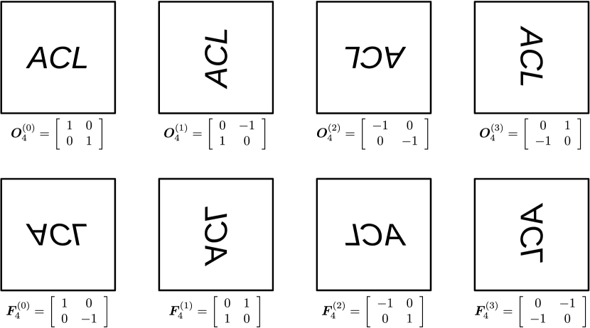
Figure 1: Elements in $\mathbb{D}_{4}$. Each subplot represents result after applying the corresponding operator to the square of ‘ACL’ on the upper left corner (on top of $\bm{O}_{4}^{(0)}$). The top row corresponds to the rotation operators and the bottom row corresponds to the reflection operators.

The element in the dihedral group $\mathbb{D}_{K}$ can be represented as 2D orthogonal matrices:

$$\bm{O}_{K}^{(m)} =\left[\begin{array}[]{cc}\cos{\left(\frac{2\pi m}{K}\right)}&-\sin{\left(\frac{2\pi m}{K}\right)}\\ \sin{\left(\frac{2\pi m}{K}\right)}&\cos{\left(\frac{2\pi m}{K}\right)}\end{array}\right]$$ (1)

$$\bm{F}_{K}^{(m)} =\left[\begin{array}[]{cc}\cos{\left(\frac{2\pi m}{K}\right)}&\sin{\left(\frac{2\pi m}{K}\right)}\\ \sin{\left(\frac{2\pi m}{K}\right)}&-\cos{\left(\frac{2\pi m}{K}\right)}\end{array}\right]$$

where $m\in\{0,1,\cdots,K\}$. Correspondingly, the group operation of dihedral group can be represented as multiplication of the representation matrices. Note that when $K$ is evenly divided by $4$, rotation matrices $\bm{O}_{K}^{(K/4)}$ and $\bm{O}_{K}^{(3K/4)}$ are skew-symmetric, and all the reflection matrices $\bm{F}_{K}^{(m)}$ and rotation matrices $\bm{O}_{K}^{(0)}$, $\bm{O}_{K}^{(K/2)}$ are symmetric. The representation of $\mathbb{D}_{4}$ is shown in Figure 1.

3 Relation Modeling with Dihedral Group and Expressiveness

	Component	Symmetric	Skew-Symmetric	Composition
				Abelian	Non-Abelian
DistMult	$r_{i}\in\mathbb{R}$	✓	$?^{*}$	✓	NA†
ComplEx	$\left[\begin{array}[]{cc}a_{i}&-b_{i}\\ b_{i}&a_{i}\end{array}\right]$	$b_{i}=0$	$a_{i}=0$	✓	NA†
ANALOGY	$\left[\begin{array}[]{cc}a_{i}&-b_{i}\\ b_{i}&a_{i}\end{array}\right]\cup\left\{c_{j}\right\}$	$b_{i}=0$	$a_{i},c_{j}=0$	✓	NA†
SimplE	$\left[\begin{array}[]{cc}0&a_{i}\\ b_{i}&0\end{array}\right]$	$a_{i}=b_{i}$	$a_{i}=-b_{i}$	NA†
DihEdral	$\mathbb{D}_{K}$	$\bm{F}_{K}^{(m)}\cup\bm{O}_{K}^{(0,K/2)}$	$\bm{O}_{K}^{(K/4,3K/4)}$	both in $\bm{O}_{K}^{(m)}$	either in $\bm{F}_{K}^{(m)}$

Table 1: Comparison on expressiveness for bilinear KB models. ‘NA’ stands for ‘not available’, and ‘✓’ stands for ‘always’. ^∗ DistMult has no skew-symmetric relation representations but it performs well in benchmark datasets because the entity type of head and tails are different. ^† The contents in column ‘Composition’ are subject to the assumption that relation composition corresponds the multiplication of the relation representation. We are not certain if there are other composition rules with which these properties are satisfied.

We propose to model the relations by the group elements in $\mathbb{D}_{K}$. Like ComplEx Trouillon et al. (2016), we assume an even number of latent dimensions $2L$. More specifically, the relation matrix takes a block diagonal form $\bm{R}={\rm diag}\left[\bm{R}^{(1)},\bm{R}^{(2)},\cdots,\bm{R}^{(L)}\right]$ where $\bm{R}^{(l)}\in\mathbb{D}_{K}$ for $l\in\{1,2,\cdots,L\}$. The corresponding embedding vectors $\bm{h}\in\mathbb{R}^{2L}$ and $\bm{t}\in\mathbb{R}^{2L}$ take the form of $\left[\bm{h}^{(1)},\cdots,\bm{h}^{(L)}\right]$ and $\left[\bm{t}^{(1)},\cdots,\bm{t}^{(L)}\right]$ where $\bm{h}^{(l)},\bm{t}^{(l)}\in\mathbb{R}^{2}$ respectively. As a result, the score for a triple $(h,r,t)$ in bilinear form can be written as a sum of these $L$ components $\bm{h}^{\top}\bm{R}\bm{t}=\sum_{l=1}^{L}\bm{h}^{(l)\top}\bm{R}^{(l)}\bm{t}^{(l)}$, We name the model DihEdral because each component $\bm{R}^{(l)}$ is a representation matrix of a dihedral group element.

Lemma 1.

The relation matrix $\bm{R}$ of DihEdral is orthogonal, i.e. $\bm{R}\bm{R}^{\top}=\bm{R}^{\top}\bm{R}=\bm{I}$.

Lemma 2.

The score of $(h,r,t)$ satisfies $\bm{h}^{\top}\bm{R}\bm{t}=-\frac{1}{2}\left(\left\|\bm{R}^{\top}\bm{h}-\bm{t}\right\|_{2}^{2}-\bm{h}^{\top}\bm{h}-\bm{t}^{\top}\bm{t}\right)$, consequently maximizing score w.r.t. $\bm{R}$ is equivalent to minimizing $\left\|\bm{R}^{\top}\bm{h}-\bm{t}\right\|_{2}^{2}$.

Theorem 1.

The relations matrices in DihEdral form a group under matrix multiplication.

Though its relation embedding takes discrete values, DihEdral is fully expressive as it is able to model relations with desired properties for each component $\bm{R}_{l}$ by the corresponding matrices in $\mathbb{D}_{K}$. The properties are summarized in Table 1, with comparison to DistMult Yang et al. (2015), ComplEx Trouillon et al. (2016), ANALOGY Liu et al. (2017) and SimplE Kazemi and Poole (2018). The details of expressiveness are described as follows. For notation convenience, we denote $\mathcal{T}^{+}$ all the possible true triples, and $\mathcal{T}^{-}$ all the possible false triples.

Symmetric

A relation $r$ is symmetric iff $(h,r,t)\in\mathcal{T}^{+}\Leftrightarrow(t,r,h)\in\mathcal{T}^{+}$. Symmetric relations in the real world include synonym, similar_to.

Note that with DihEdral, the component $\bm{R}_{l}$ can be a reflection matrix which is symmetric and off-diagonal. This is in contrast to DistMult and ComplEx where the relation matrix has to be diagonal when it is symmetric at the same time.

Skew-Symmetric

A relation $r$ is skew-symmetric iff $(h,r,t)\in\mathcal{T}^{+}\Leftrightarrow(t,r,h)\in\mathcal{T}^{-}$. Skew-symmetric relations in the real world include father_of, member_of.

When $K$ is a multiple of $4$, pure skew-symmetric matrices in $\mathbb{D}_{4}$ can be chosen. As a result, the relation is guaranteed to be skew-symmetric satisfying $\phi(h,r,t)=-\phi(t,r,h)$.

Inversion

$r_{2}$ is the inverse of $r_{1}$ iff $(h,r_{1},t)\in\mathcal{T}^{+}\Leftrightarrow(t,r_{2},h)\in\mathcal{T}^{+}$. As a real world example, parent_of is the inversion of child_of.

The inverse of the relation $r$ is represented by $\bm{R}^{-1}$ in an ideal situation: For two positive triples $(h,r_{1},t)$ and $(t,r_{2},h)$, we have $\bm{R}_{1}^{\top}\bm{h}\approx\bm{t}$ and $\bm{R}_{2}^{\top}\bm{t}\approx\bm{h}$ in an ideal situation (cf. Lemma 2), With enough occurrences of pair $\{h,t\}$ we have $\bm{R}_{2}=\bm{R}_{1}^{-1}$.

Composition

$r_{3}$ is composition of $r_{1}$ and $r_{2}$, denoted as $r_{3}=r_{1}\odot r_{2}$ iff $(h,r_{1},m)\in\mathcal{T}^{+}\wedge(m,r_{2},t)\in\mathcal{T}^{+}\Leftrightarrow(h,r_{3},t)\in\mathcal{T}^{+}$. Example of composition in the real world includes nationality = born_in_city $\odot$ city_belong_to_nation. Depending on the commutative property, there are two cases of relation compositions:

• Abelian $r_{1}$ and $r_{2}$ are Abelian if $(h,r_{1}\odot r_{2},t)\in\mathcal{T}^{+}\Leftrightarrow(h,r_{2}\odot r_{1},t)\in\mathcal{T}^{+}$. Real world example includes opposite_gender $\odot$ profession $=$ profession $\odot$ opposite_gender.

• Non-Abelian $r_{1}$ and $r_{2}$ are non-Abelian if $(h,r_{1}\odot r_{2},t)\in\mathcal{T}^{+}\nLeftrightarrow(h,r_{2}\odot r_{1},t)\in\mathcal{T}^{+}$. Real world example include parent_of $\odot$ spouse_of $\neq$ spouse_of $\odot$ parent_of.

In DihEdral, the relation composition operator $\odot$ corresponds to the matrix multiplication of the corresponding representations, i.e. $\bm{R}_{3}\approx\bm{R}_{1}\bm{R}_{2}$. Consider three positive triples $(h,r_{1},m)$, $(m,r_{2},t)$ and $(h,r_{3},t)$. In the ideal situation, we have $\bm{R}_{1}^{\top}\bm{h}\approx\bm{m}$, $\bm{R}_{2}^{\top}\bm{m}\approx\bm{t}$, $\bm{R}_{3}^{\top}\bm{h}\approx\bm{t}$ (cf. Lemma 2), and further $\bm{R}_{2}^{\top}\bm{R}_{1}^{\top}\bm{h}\approx\bm{t}$. With enough occurrences of such $\{h,t\}$ pairs in the training dataset, we have $\bm{R}_{3}\approx\bm{R}_{1}\bm{R}_{2}$.

Note that although all the rotation matrices form a subgroup to dihedral group, and hence algebraically closed, the rotation subgroup could not model non-Abelian relations. To model non-Abelian relation compositions at least one reflection matrix should be involved.

4 Training

In the standard traing framework for KG embedding models, parameters $\Theta=\Theta_{\mathcal{E}}\cup\Theta_{\mathcal{R}}$, i.e. the union of entity and relation embeddings, are learnt by stochastic optimization methods. For each minibatch of positive triples, a small number of negative triples are sampled by corrupting head or tail for each positive triple, then related parameters in the model are updated by minimizing the binary negative log-likelihood such that positive triples will get higher scores than negative triples. Specifically, the loss function is written as follows,

$$\min_{\Theta}\sum_{(h,r,t)\in\mathcal{T}^{+}\cup\mathcal{T}^{-}}-\log\sigma\left(y\phi(h,r,t)\right)+\lambda||\Theta_{\mathcal{E}}||^{2},$$ (2)

where $\lambda\in\mathbb{R}$ is the $L_{2}$ regularization coefficient for entity embeddings only, $\mathcal{T}^{+}$ and $\mathcal{T}^{-}$ are the sets of positive and sampled negative triples in a minibatch, and $y$ equals to $1$ if $(h,r,t)\in\mathcal{T}^{+}$ otherwise $-1$. $\sigma$ is a sigmoid function defined as $\sigma(x)=1/(1+\exp(-x))$.

Special treatments of the relation representations $\bm{R}$ are required as they takes discrete values. In the next subsections we describe a reparametrization method for general $K$, followed by a simple approach when $K$ takes small integers values. With these treatments, DihEdral could be trained within the standard framework.

4.1 Gumbel-Softmax Approach

Each relation component $\bm{R}^{(l)}$ can be parametrized with a one-hot variable $\bm{c}^{(l)}\in\{0,1\}^{2K}$ encoding $2K$ choices of matrices in $\mathbb{D}_{K}$: $\bm{R}^{(l)}=\sum_{k=1}^{2K}c^{(l)}_{k}\bm{D}_{k}$ where $\{\bm{D}_{k},k\in\{1,\cdots,2K\}\}$ enumerates $\mathbb{D}_{K}$. The number of parameters for each relation is $2LK$ in this approach.

One-hot variable $\bm{c}^{(l)}$ is further parametrized by $\bm{s}^{(l)}\in\mathbb{R}^{2K}$ by Gumbel trick Jang et al. (2017) with the following steps: 1) take i.i.d. samples $q_{1},q_{2},\dots,q_{2K}$ from a Gumbel distribution: $q_{i}=-\log(-\log u_{i})$, where $u_{i}\sim\mathcal{U}(0,1)$ are samples from a uniform distribution; 2) use log-softmax form of $\bm{s}^{(l)}$ to parametrize $\bm{c}^{(l)}\in\{0,1\}^{2K}$:

$$c^{(l)}_{k}=\frac{\exp\left[(s^{(l)}_{k}+q_{k})/\tau\right]}{\sum_{k=1}^{2K}\exp\left[(s^{(l)}_{k}+q_{k})/\tau\right]}$$ (3)

where $\tau$ is the tunable temperature. During training, we start with high temperature, e.g. $\tau_{0}=3$, to drive the system out of pool local minimums, and gradually cool the system with $\tau=\max(0.5,\tau_{0}\exp(-0.001t))$ where $t$ is the number of epochs elapsed.

4.2 Reparametrization with Binary Variables

Another parametrization technique for $\mathbb{D}_{K}$ where $K\in\{4,6\}$ is to parametrize each element in the matrix $\bm{R}^{(l)}$ directly. Specifically we have

$$\bm{R}^{(l)}=\left[\begin{array}[]{cc}\lambda&-\alpha\gamma\\ \gamma&\alpha\lambda\\ \end{array}\right],$$

where $\lambda=\cos(2\pi k/K)$, $\gamma=\sin(2\pi k/K)$, $k\in\{0,1,\cdots,2K-1\}$ and $\alpha\in\{-1,1\}$ is the reflection indicator . Both $\lambda$ and $\gamma$ can be parametrized by the same set of binary variables $\{x,y,z\}$:

$$\lambda =\begin{cases}(x+y)/2&K=4\\ y(3-x)/4&K=6\end{cases},$$

$$\gamma =\begin{cases}(x-y)/2&K=4\\ z(x+1)\sqrt{3}/4&K=6\end{cases}.$$

In the forward pass, each binary variable $b\in\{x,y,z\}$ is parametrized by taking a element-wise sign function of a real number: $b=\mathrm{sign}(b_{\mathrm{real}})$ where $b_{\mathrm{real}}\in\mathbb{R}$.

In the backward pass, since the original gradient of sign function is almost zero everywhere such that $b_{\mathrm{real}}$ will not be activated, the gradient of loss with respect to the real variable is estimated with the straight-through estimator (STE) Yin et al. (2019). The functional form for STE is not unique and worth profound theoretical study. In our experiments, we used identity STE Bengio et al. (2013):

$$\frac{\partial\mathrm{loss}}{\partial b_{\mathrm{real}}}=\frac{\partial\mathrm{loss}}{\partial b}\mathds{1},$$

where $\mathds{1}$ stands for element-wise identity.

For these two approaches, we name the model as D$K$-Gumbel for Gumbel-Softmax approach and D$K$-STE for reparametrization using binary variable approach.

5 Experimental Result

This section presents our experiments and results. We first introduce the benchmark datasets used in our experiments, after that we evaluate our approach in the link prediction task.

5.1 Datasets

Introduced in Bordes et al. (2013), WN18 and FB15K are popular benchmarks for link prediction tasks. WN18 is a subset of the famous WordNet database that describes relations between words. In WN18 the most frequent types of relations form reversible pairs (e.g., hypernym to hyponym, part_of to has_part). FB15K is a subsampling of Freebase limited to 15k entities, introduced in Bordes et al. (2013). It contains triples with different characteristics (e.g., one to-one relations such as capital_of to many-to-many such as actor_in_film). YAGO3-10 Dettmers et al. (2018) is a subset of YAGO3 Suchanek et al. (2007) with each entity contains at least 10 relations.

As noted in Toutanova et al. (2015); Dettmers et al. (2018), in the original WN18 and FB15k datasets there are a large amount of test triples appear as reciprocal form of the training samples, due to the reversible relation pairs. Therefore, these authors eliminated the inverse relations and constructed corresponding subsets: WN18RR with 11 relations and FB15K-237 with 237 relations, both of which are free from test data leak. All datasets statistics are shown in Table 2.

Dataset	$|\mathcal{E}|$	$|\mathcal{R}|$	Train	Valid	Test
WN18	41k	18	141k	5k	5k
WN18RR	41k	11	87k	3k	3k
FB15K	15k	1.3k	483k	50k	59k
FB15K-237	15k	237	273k	18k	20k
YAGO3-10	123k	37	1M	5k	5k

Table 2: Statistics of Datasets.

5.2 Evaluation Metric

We use the popular metrics filtered HITS@1, 3, 10 and mean reciprocal rank (MRR) as our evaluation metrics as in Bordes et al. (2013).

	WN18				FB15K
	HITS@N			MRR	HITS@N			MRR
	1	3	10		1	3	10
TransE† Bordes et al. (2013)	8.9	82.3	93.4	45.4	23.1	47.2	64.1	22.1
DistMult† Yang et al. (2015)	72.8	91.4	93.6	82.2	54.6	73.3	82.4	65.4
ComplEx† Trouillon et al. (2016)	93.6	94.5	94.7	94.1	59.9	75.9	84.0	69.2
HolE Nickel et al. (2016)	93.0	94.5	94.7	93.8	40.2	61.3	73.9	52.4
ANALOGY Liu et al. (2017)	93.9	94.4	94.7	94.2	64.6	78.5	85.4	72.5
Single DistMult Kadlec et al. (2017)	—	—	94.6	79.7	—	—	89.3	79.8
SimplE Kazemi and Poole (2018)	93.9	94.4	94.7	94.2	66.0	77.3	83.8	72.7
R-GCN Schlichtkrull et al. (2018)	69.7	92.9	96.4	81.9	60.1	76.0	84.2	69.6
ConvE Dettmers et al. (2018)	93.5	94.6	95.6	94.3	55.8	72.3	83.1	65.7
D4-STE	94.2	94.8	95.2	94.6	64.1	80.3	87.7	73.3
D4-Gumbel	94.2	94.9	95.4	94.6	64.8	78.2	86.4	72.8

Table 3: Link prediction results on WN18 and FB15K datasets. Results marked by ‘$\dagger$’ are taken from Trouillon et al. (2016), and the rest of the results are taken from original literatures.

5.3 Model Selection and Hyper-parameters

We implemented DihEdral in PyTorch Paszke et al. (2017). In all our experiments, we selected the hyperparameters of our model in a grid search setting for the best MRR in the validation set. We trained DK-Gumbel for $K\in\{4,6,8\}$ and DK-STE for $K\in\{4,6\}$ with AdaGrad optimizer Duchi et al. (2011), and we didn’t notice significant difference in terms of the evaluation metrics when varying $K$. In the following we only report the result for $K=4$.

For D4-Gumbel, we performed grid search for the $L_{2}$ regularization coefficient $\lambda$ $\in[10^{-5},10^{-4},10^{-3}]$ and learning rate $\in[0.5,1]$. For D4-STE, hyperparamter ranges for the grid search were as follows: $\lambda$ $\in$ [0.001, 0.01, 0.1, 0.2], learning rate $\in$ [0.01, 0.02, 0.03, 0.05, 0.1]. For both settings we performed grid search with batch sizes $\in$ [512, 1024, 2048] and negative sample ratio $\in$ [1, 6, 10]. We used embedding dimension $2L=1500$ for FB15K, $2L=600$ for both FB15K-237 and YAGO3-10, $2L=200$ for WN18 and WN18RR. We used the standard train/valid/test splits provided with these datasets.

	WN18RR				FB15K-237				YAGO3-10
	HITS@N			MRR	HITS@N			MRR	HITS@N			MRR
	1	3	10		1	3	10		1	3	10
DistMult†	39.0	44.0	49.0	43.0	15.5	26.3	41.9	24.1	24.0	38.0	54.0	34.0
ComplEx†	41.0	46.0	51.0	44.0	15.8	27.5	42.8	24.7	26.0	40.0	55.0	36.0
R-GCN	—	—	—	—	15.1	26.4	41.7	24.8	—	—	—	—
ConvE†	40.0	44.0	52.0	43.0	23.7	35.6	50.1	32.5	35.0	49.0	62.0	44.0
MINERVA∗	41.3	45.6	51.3	44.8	21.7	32.9	45.6	29.3	—	—	—	—
D4-STE	45.2	49.1	53.6	48.0	23.0	35.3	50.2	32.0	38.1	52.3	64.3	47.2
D4-Gumbel	44.2	50.5	55.7	48.6	20.4	33.2	49.6	30.0	29.4	43.6	57.3	38.8

Table 4: Link prediction results on WN18RR and FB15K-237 datasets. Results marked by ‘$\dagger$’ are taken from Dettmers et al. (2018), and result marked by ‘$*$’ is taken from Das et al. (2018).

The results of link predictions are shown in Table 3 and 4, where the results for the baselines are directly taken from original literature. DihEdral outperforms almost all models in bilinear form, and even ConvE in FB15K, WN18RR and YAGO3-10. The result demonstrates that even DihEdral takes discretized value in relation representations, proper modeling the underlying structure of relations using $\mathbb{D}_{K}$ is essential.

6 Case Studies

The learned representation from DihEdral is not only able to reach the state-of-the-art performance in link prediction tasks, but also provides insights with its special properties. In this section, we present the detailed case studies on these properties. In order to achieve better resolutions, we increased the embedding dimension to $2L=600$ for WN18 datasets.

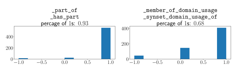
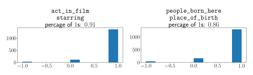
Figure 2: Relation inversion in WN18 (top) and FB15K (bottom). Each subplot shows the histogram of diagonal elements in $\bm{R}_{1}\bm{R}_{2}$ where $r_{1}$ is inverse relation of $r_{2}$. The name of the two relations and the percentage of the $1$s in the diagonal are shown in the first, second and third row of the subplot title, respectively.

6.1 Inversion

We show the multiplication of some pairs of inversion relations on WN18 and FB15K in Figure 2, and the result is close to an identity matrix. For the relation pair {_member_of_domain_usage, _synset_domain_usage_of}, the multiplication deviates from ideal identity matrix as the performance for these two relations are poorer compared to the others. We also repeat the same case study for other bilinear embedding methods, however their multiplications are not identity, but close to diagonal matrices with different elements.

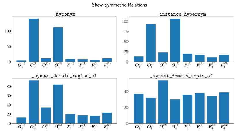
Figure 3: Historgram of each component of $\mathbb{D}_{4}$ for WN18. The top and bottom row corresponds to symmetric and skew-symmetric relations, respectively. Note that $\bm{O}_{4}^{(1,3)}$ are skew-symmetric components and others are symmetric.

6.2 Symmetry and Skew-Symmetry

Since the KB datasets do not contain negative triples explicitly, there is no penalty to model skew-symmetric relations with symmetric matrices. This is perhaps the reason why DistMult performs well on FB15K dataset in which a lot of relations are skew-symmetric.

To resolve this ambiguity, for each positive triple $(h,r,t)$ with a definite skew-symmetric relation $r$, a negative triple $(t,r,h)$ is sampled with probability 0.5. After adding this new negative sampling scheme in D4-Gumbel, the symmetric and skew-symmetric relations can be distinguished on WN18 dataset without reducing performance on link prediction tasks. Figure 3 shows that both symmetric and skew-symmetric relations favor corresponding components in $\mathbb{D}_{4}$ as expected. Again, due to imperfect performance of _synset_domain_topic_of, its corresponding representation is imperfect as well. We also conduct the same experiment without adding this sampling scheme, the histogram for the symmetric relations are similar, but there is no strong preference for skew-symmetric relations.

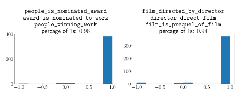
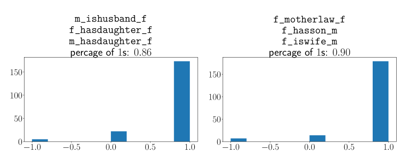
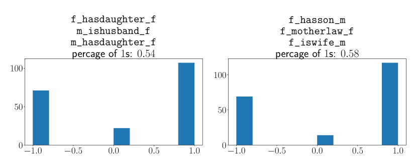
Figure 4: Relation composition on FB15K-237 and FAMILY. Each subplot shows the histogram of diagonal elements in $\bm{R}_{1}\bm{R}_{2}\bm{R}_{3}^{-1}$ where $r_{3}$ is treated as the composition of $r_{1}$ and $r_{2}$. The name of the three relations and the percentage of the $1$s in the diagonal are shown in the 1st, 2nd, 3rd and 4th line of subplot title. The two subplots in the first rows shows composition for FB15K-237, and subplots on the second and third row are used to check composition and non-Abelian on FAMILY.

6.3 Relation Composition

In FB15K-237 dataset the majority of patterns is relation composition. However, these compositions are Abelian only because all the inverse relations are filtered out on purpose. To justify if non-Abelian relation compositions can be discovered by DihEdral in an ideal situation, we generate a synthetic dataset called FAMILY. Specifically, we first generated two generations of people with equal number of male and females in each generation, and randomly assigned spouse edges within each generation and child and parent edges between the two generations, after which the sibling, parent_in_law and child_in_law edges are connected based on commonsense logic.

We trained D4-Gumbel on FAMILY with latent dimension $2L=400$. In addition to the loss in Eq. 2, we add the following regularization term to encourage the score of positive triple to be higher than that of negative triple for each component independently.

$$-\sum_{l=1}^{L}\log\sigma\left(\bm{h}^{(l)\top}\bm{R}^{(l)}\bm{t}^{(l)}-\bm{h}^{*(l)\top}\bm{R}^{(l)}\bm{t}^{*(l)}\right).$$

where $(h,r,t)\in\mathcal{T}^{+}$, and the corresponding negative triple $(h^{*},r,t^{*})\in\mathcal{T}^{-}$.

For each composition $r_{3}=r_{1}\odot r_{2}$, we compute the histogram of $\bm{R}_{1}\bm{R}_{2}\bm{R}_{3}^{-1}$ . The result for relation compositions in FB15K-237 and FAMILY is shown in Figure 4, from which we could see good composition as matrix multiplication. We also reveal the non-Abelian property in FAMILY by exchanging the order of $r_{1}$ and $r_{2}$.

7 Related Works

In this section we discuss the related works and their connections to our approach.

TransE Bordes et al. (2013) takes relations as a translating operator between head and tail entities. More complicated distance functions Wang et al. (2014); Lin et al. (2015b, a) are also proposed as extensions to TransE. TorusE Ebisu and Ichise (2018) proposed a novel distance function defined over a torus by transform the vector space by an Abelian group onto a $n$-dimensional torus. ProjE Shi and Weninger (2017) designs a neural network with a combination layer and a projection layer. R-GCN Schlichtkrull et al. (2018) employs convolution over multiple entities to capture spectrum of the knowledge graph. ConvE Dettmers et al. (2018) performs 2D convolution on the concatenation of entity and relation embeddings, thus by nature introduces non-linearity to enhance expressiveness.

In RESCAL Nickel et al. (2011) each relation is represented by a full-rank matrix. As a downside, there is a huge number of parameters in RESCAL making the model prone to overfitting. A totally symmetric DistMult Yang et al. (2015) model simplifies RESCAL by representing each relation with a diagonal matrix. To parametrize skew-symmetric relations, ComplEx Trouillon et al. (2016) extends DistMult by using complex-valued instead of real-valued vectors for entities and relations. The representation matrix of ComplEx supports both symmetric and skew-symmetric relations while being closed under matrix multiplication. HolE Nickel et al. (2016) models the skew-symmetry with circular correlation between entity embeddings, thus ensures shifts in covariance between embeddings at different dimensions. It was recently showed that HolE is isomophic to ComplEx Hayashi and Shimbo (2017). ANALOGY Liu et al. (2017) and SimplE Kazemi and Poole (2018) both reformulate the tensor decomposition approach in light of analogical and reversible relations.

Though embedding based approach achieves state-of-the-art performance on link prediction task, symbolic relation composition is not explicitly modeled. In contrast, the latter goal is currently popularized by directly modeling the reasoning paths Neelakantan et al. (2015); Xiong et al. (2017); Das et al. (2018); Lin et al. (2018); Guo et al. (2019). As paths are consistent with reasoning logic structure, non-Abelian composition is supported by nature.

DihEdral is more expressive when compared to other bilinear form based embedding methods such as DistMult, ComplEX and ANALOGY. As the relation matrix is restricted to be orthogonal, DihEdral could bridge translation based and bilinear form based approaches as the training objective w.r.t. the relation matrix is similar (cf Lemma 2). Besides, DihEdral is the first embedding method to incorporate non-Abelian relation compositions in terms of matrix multiplications (cf. Theorem 1).

8 Conclusion

This paper proposed DihEdral for KG relation embedding. By leveraging the desired properties of dihedral group, relation (skew-) symmetry, inversion, and (non-) Abelian compositions are all supported. Our experimental results on benchmark KGs showed that DihEdral outperforms existing bilinear form models and even deep learning methods. Finally, we demonstrated that the above g properties can be learned from DihEdral by extensive case studies, yielding a substantial increase in interpretability from existing models.

References

- Bengio et al. (2013) Yoshua Bengio, Nicholas Léonard, and Aaron C. Courville. 2013. Estimating or propagating gradients through stochastic neurons for conditional computation. arXiv preprint arXiv:1308.3432.
- Berant et al. (2013) Jonathan Berant, Andrew Chou, Roy Frostig, and Percy Liang. 2013. Semantic parsing on Freebase from question-answer pairs. In Proceedings of EMNLP.
- Bordes et al. (2014) Antoine Bordes, Sumit Chopra, and Jason Weston. 2014. Question answering with subgraph embeddings. In Proceedings of EMNLP.
- Bordes et al. (2013) Antoine Bordes, Nicolas Usunier, Alberto Garcia-Duran, Jason Weston, and Oksana Yakhnenko. 2013. Translating embeddings for modeling multi-relational data. In Proceedings of NeurIPs.
- Das et al. (2018) Rajarshi Das, Shehzaad Dhuliawala, Manzil Zaheer, Luke Vilnis, Ishan Durugkar, Akshay Krishnamurthy, Alex Smola, and Andrew McCallum. 2018. Go for a walk and arrive at the answer: Reasoning over paths in knowledge bases using reinforcement learning. In Proceedings in ICLR.
- Dettmers et al. (2018) Tim Dettmers, Pasquale Minervini, Pontus Stenetorp, and Sebastian Riedel. 2018. Convolutional 2d knowledge graph embeddings. In Proceedings of AAAI.
- Duchi et al. (2011) John Duchi, Elad Hazan, and Yoram Singer. 2011. Adaptive subgradient methods for online learning and stochastic optimization. J. Mach. Learn. Res., 12:2121–2159.
- Ebisu and Ichise (2018) Takuma Ebisu and Ryutaro Ichise. 2018. TorusE: Knowledge graph embedding on a lie group. In Proceedings of AAAI.
- Guo et al. (2019) Lingbing Guo, Zequn Sun, and Wei Hu. 2019. Learning to exploit long-term relational dependencies in knowledge graphs. In Proceedings of ICML.
- Guu et al. (2015) Kelvin Guu, John Miller, and Percy Liang. 2015. Traversing knowledge graphs in vector space. In Proceedings of EMNLP.
- Hayashi and Shimbo (2017) Katsuhiko Hayashi and Masashi Shimbo. 2017. On the equivalence of holographic and complex embeddings for link prediction. In Proceedings of ACL.
- He et al. (2017) He He, Anusha Balakrishnan, Mihail Eric, and Percy Liang. 2017. Learning symmetric collaborative dialogue agents with dynamic knowledge graph embeddings. In Proceedings of ACL.
- Jang et al. (2017) Eric Jang, Shixiang Gu, and Ben Poole. 2017. Categorical reparameterization with gumbel-softmax. In Proceedings of ICLR.
- Kadlec et al. (2017) Rudolf Kadlec, Ondrej Bajgar, and Jan Kleindienst. 2017. Knowledge base completion: Baselines strike back. In Proceedings of the 2nd Workshop on Representation Learning for NLP.
- Kazemi and Poole (2018) Seyed Mehran Kazemi and David Poole. 2018. SimplE embedding for link prediction in knowledge graphs. In Proceedings of NeurIPs.
- Lin et al. (2018) Xi Victoria Lin, Richard Socher, and Caiming Xiong. 2018. Multi-hop knowledge graph reasoning with reward shaping. In Proceedings in EMNLP.
- Lin et al. (2015a) Yankai Lin, Zhiyuan Liu, Huan-Bo Luan, Maosong Sun, Siwei Rao, and Song Liu. 2015a. Modeling relation paths for representation learning of knowledge bases. In Proceedings of EMNLP.
- Lin et al. (2015b) Yankai Lin, Zhiyuan Liu, Maosong Sun, Yang Liu, and Xuan Zhu. 2015b. Learning entity and relation embeddings for knowledge graph completion. In Proceedings of AAAI.
- Liu et al. (2017) Hanxiao Liu, Yuexin Wu, and Yiming Yang. 2017. Analogical inference for multi-relational embeddings. In Proceedings of ICML.
- Neelakantan et al. (2015) Arvind Neelakantan, Benjamin Roth, and Andrew McCallum. 2015. Compositional vector space models for knowledge base completion. In Proceedings of ACL.
- Nickel et al. (2016) Maximilian Nickel, Lorenzo Rosasco, and Tomaso Poggio. 2016. Holographic embeddings of knowledge graphs. In Proceedings of AAAI.
- Nickel et al. (2011) Maximilian Nickel, Volker Tresp, and Hans-Peter Kriegel. 2011. A three-way model for collective learning on multi-relational data. In Proceedings of ICML.
- Paszke et al. (2017) Adam Paszke, Sam Gross, Soumith Chintala, Gregory Chanan, Edward Yang, Zachary DeVito, Zeming Lin, Alban Desmaison, Luca Antiga, and Adam Lerer. 2017. Automatic differentiation in PyTorch. In Proceedings of NIPS Autodiff Workshop.
- Schlichtkrull et al. (2018) Michael Sejr Schlichtkrull, Thomas N. Kipf, Peter Bloem, Rianne van den Berg, Ivan Titov, and Max Welling. 2018. Modeling relational data with graph convolutional networks. arXiv preprint arXiv:1703.06103.
- Shi and Weninger (2017) Baoxu Shi and Tim Weninger. 2017. ProjE: Embedding projection for knowledge graph completion. In Proceedings of AAAI.
- Socher et al. (2013) Richard Socher, Danqi Chen, Christopher D. Manning, and Andrew Y. Ng. 2013. Reasoning with neural tensor networks for knowledge base completion. In Proceedings of NeurIPs.
- Steinberg (2012) Benjamin Steinberg. 2012. Representation Theory of Finite Groups. Springer-Verlag New York.
- Suchanek et al. (2007) Fabian M. Suchanek, Gjergji Kasneci, and Gerhard Weikum. 2007. YAGO: A core of semantic knowledge. In Proceedings of WWW.
- Toutanova et al. (2015) Kristina Toutanova, Danqi Chen, Patrick Pantel, Hoifung Poon, Pallavi Choudhury, and Michael Gamon. 2015. Representing text for joint embedding of text and knowledge bases. In Proceedings of EMNLP.
- Trouillon et al. (2016) Théo Trouillon, Johannes Welbl, Sebastian Riedel, Éric Gaussier, and Guillaume Bouchard. 2016. Complex embeddings for simple link prediction. In Proceedings of ICML.
- Wang et al. (2014) Zhen Wang, Jianwen Zhang, Jianlin Feng, and Zheng Chen. 2014. Knowledge graph embedding by translating on hyperplanes. In Proceedings of AAAI.
- Xiong et al. (2017) Wenhan Xiong, Thien Hoang, and William Yang Wang. 2017. DeepPath: A reinforcement learning method for knowledge graph reasoning. In Proceedings in EMNLP.
- Yang et al. (2015) Bishan Yang, Wen-tau Yih, Xiaodong He, Jianfeng Gao, and Li Deng. 2015. Embedding entities and relations for learning and inference in knowledge bases. In Proceedings of ICLR.
- Yin et al. (2019) Penghang Yin, Jiancheng Lyu, Shuai Zhang, Stanley J. Osher, Yingyong Qi, and Jack Xin. 2019. Understanding straight-through estimator in training activation quantized neural nets. In Proceedings of ICLR.