CO observations of major merger pairs at z=0: Molecular gas mass and star formation

We present CO observations of 78 spiral galaxies in local merger pairs. These galaxies represent a subsample of a K_s-band selected sample consisting of 88 close major-merger pairs (HKPAIRs), 44 spiral-spiral (S+S) pairs and 44 spiral-elliptical (S+E) pairs, with separation $<20\,h^{-1}$ kpc and mass ratio $<$ 2.5. For all objects, the star formation rate (SFR) and dust mass were derived from Herschel PACS and SPIRE data, and the atomic gas mass, $M_{\rm HI}$, from the Green Bank Telescope HI observations. The complete data set allows us to study the relation between the gas (atomic and molecular) mass, dust mass and SFR in merger galaxies. We derive the molecular gas fraction ($M_{{\rm H}_{2}}$/$M_{{\rm*}}$), molecular-to-atomic gas mass ratio ($M_{{\rm H}_{2}}$/$M_{\rm HI}$), gas-to-dust mass ratio and SFE (=SFR/$M_{{\rm H}_{2}}$) and study their dependences on pair type (S+S compared to S+E), stellar mass and the presence of morphological interaction signs. We find an overall moderate enhancements ($\sim 2\times$) in both molecular gas fraction ($M_{{\rm H}_{2}}$/$M_{{\rm*}}$), and molecular-to-atomic gas ratio ($M_{{\rm H}_{2}}$/$M_{\rm HI}$) for star-forming galaxies in major-merger pairs compared to non-interacting comparison samples, whereas no enhancement was found for the SFE nor for the total gas mass fraction (($M_{\rm HI}$+$M_{{\rm H}_{2}}$)/$M_{{\rm*}}$). When divided into S+S and S+E, low mass and high mass, and with and without interaction signs, there is a small difference in SFE, moderate difference in $M_{{\rm H}_{2}}$/$M_{{\rm*}}$, and strong differences in $M_{{\rm H}_{2}}$/$M_{\rm HI}$  between subsamples. For the molecular-to-atomic gas ratio $M_{{\rm H}_{2}}$/$M_{\rm HI}$, the difference between S+S and S+E subsamples is $0.69\pm 0.16$ dex and between pairs with and without interaction signs is $0.53\pm 0.18$ dex. Together, our results suggest (1) star formation enhancement in close major-merger pairs occurs mainly in S+S pairs after the first close encounter (indicated by interaction signs) because the HI gas is compressed into star-forming molecular gas by the tidal torque; (2) this effect is much weakened in the S+E pairs.

1 Introduction

Gravitational interaction is an important process for the evolution of galaxies in clusters (Dressler 1980; Moore et al. 1996), groups (Hickson et al. 1992; Lisenfeld et al. 2017), triplets (Duplancic et al. 2015; Argudo-Fernández et al. 2015) and pairs (Ellison et al. 2010; Argudo-Fernández et al. 2015). It is now well established that galaxy interactions in pairs can cause an enhancement of the star formation rate (SFR). The amount of the enhancement depends on parameters of the galaxies (mass ratio, gas fraction), on the orbital parameters of the interacting galaxies (e.g., Kennicutt et al. 1987; Xu & Sulentic 1990). and on the phase of the interaction (e.g., Di Matteo et al. 2007; Cox et al. 2008; Scudder et al. 2012). The largest enhancement of the SFR occurs in equal-mass mergers (major mergers) after the first pericenter and, much stronger, during coalescene (e.g., Nikolic et al. 2004; Scudder et al. 2012). In most cases the SFR enhancement is only moderate ($<$ factor of 5 in 85% of the cases, di Matteo et al. 2008), but when all parameters are favourable (gas rich, equal mass galaxies during coalescence) short episodes of very high SFR can occur, the most extreme examples being (Ultra) Luminous Infrared galaxies (Sanders & Mirabel 1996; Ellison et al. 2013).

Simulations of galaxy mergers have helped to improve our understanding of the processes that affect the SFR during a merger. It has long been recognized that tidal forces can produce an increase of the SFR (see Barnes & Hernquist 1992). Gravitational torques produced by asymmetric tidal forces cause the gas at large radii to lose angular momentum and fall into the central regions where the high gas surface density produces a central starburst. High resolution simulations have shown, that, in addition, changes in the substructure of the Interstellar Medium (ISM) can favor the collapse of molecular clouds and thus enhance the SFR (Teyssier et al. 2010). Parsec-resolution simulations of Renaud et al. (2014) find that during a typical galaxy merger tidal compression can increase and modify turbulence, leading to an excess of dense gas and an enhancement in the SF activity and the SF efficiency (SFE = SFR/$M_{{\rm H}_{2}}$).

In order to observationally better understand the question of when and how SF is enhanced during the merging process, Domingue et al. (2009) selected, based on the K_s-band, a sample of close major mergers (KPAIR sample). Xu et al. (2010) studied the specific SFR (sSFR=SFR/$M_{{\rm*}}$) enhancement in this sample and found enhancement in galaxies in spiral-spiral (S+S) pairs, but none in spiral-elliptical (S+E) pairs. This result was confirmed by Cao et al. (2016) for an extended sample (H-KPAIR sample) based on Herschel PACS and SPIRE data. These data allowed them to derive the SFR and dust mass which can be used as an indicator of the total gas mass, assuming a constant dust-to-gas mass ratio. They found an increase in the SFE_gas(= SFR/$M_{{\rm gas}}$) of spirals in S+S pairs, whereas the value in spirals in S+E pairs is the same as for a control sample. The difference between the gas fraction ($M_{{\rm gas}}$/$M_{{\rm*}}$) in star forming galaxies in S+S and S+E pairs is weak ($\sim$40%) and insignificant, indicating that the amount of gas is not the reason for this difference. Using WISE and Herschel  data, Domingue et al. (2016) found that spirals in S+S pairs exhibit a significant enhancement in the interstellar radiation field and dust temperature, while spirals in S+E pairs do not. Zuo et al. (2018) observed the sample in HI with the Green Bank Telescope and found a difference in SFE_HI (=SFR/$M_{\rm HI}$) between S+S and S+E pairs.

Molecular gas is more closely related to the process of SF than the HI gas. The SFR can be enhanced by a larger amount of molecular gas from which stars form, or by making the process of star formation from gas more efficient (i.e. increasing SFE), e.g. by increasing the gas density. Both scenarios can be distinguished observationally by measuring the molecular gas mass (compared to the stellar or atomic gas mass) and the SFE. The role of the molecular gas in galaxy interactions has been investigated in numerous studies. There is a general consensus that the molecular gas content is enhanced in interacting galaxies. This has already been seen in the first studies with samples ranging from $\sim$ 10 to 1000 galaxies (Braine & Combes 1993; Combes et al. 1994; Casasola et al. 2004), and has been confirmed in more recent studies. Violino et al. (2018) found for a small sample of 9 nearby galaxies which they compared to a well-matched comparison sample that both the molecular gas fraction ($M_{{\rm H}_{2}}$/$M_{{\rm*}}$) and the SFE are enhanced in the interacting sample. Both parameters are, however, consistent with non-mergers of similarly enhanced SFR. Pan et al. (2018) investigated a sample of 58 pairs and found an enhancement of the SFR, SFE, $M_{{\rm H}_{2}}$ and $M_{{\rm H}_{2}}$/$M_{{\rm*}}$. Whereas the enhancement of the SFR, $M_{{\rm H}_{2}}$and $M_{{\rm H}_{2}}$/$M_{{\rm*}}$ increases with decreasing pair separation, the SFE is only enhanced in close (separation $<$ 20 kpc) pairs and equal mass systems. An enhancement of the SFE was found in the earlier studies only in strongly interacting galaxies (Solomon & Sage 1988; Sofue et al. 1993) whereas more weakly interacting pairs did not show any enhancement (Solomon & Sage 1988). No enhancement in the SFE was found in studies with mixed interacting samples (Combes et al. 1994; Casasola et al. 2004), whereas the more recent studies (Violino et al. 2018; Pan et al. 2018) did find a small ($\lesssim$ factor of 2) increase in the SFE.

In the present paper we present new CO data for a subsample of H-KPAIR, which includes only close major mergers (r$<20h^{-1}$ kpc, mass ratio $<$ 2.5). These data allow us to calculate and analyse the molecular gas content in a homogenous sample with a large ancillary data set. Together with the data from Cao et al. (2016) and Zuo et al. (2018) we now have a complete data set to study the relation between the cold interstellar medium (atomic, molecular gas and dust) and SF. This sample allows us to analyse this relation as a function of pair type (S+S or S+E), stellar mass and interaction stage classified by the morphology. The goal of the present paper is to better understand how SF is enhanced in the merging process, and what role the gas, in particular the molecular component, plays.

Throughout this paper, we adopt the $\Lambda$-cosmology with $\Omega_{\rm m}=0.3$ and $\Omega_{\rm\Lambda}=0.7$ and $H_{\rm 0}=70$ km s^-1 Mpc^-1.

2 The sample

The local galaxy pair sample used in this work was constructed from the KPAIR sample which is a complete and unbiased K_s-band (2.16 $\mu$m) selected sample of 170 close major-merger galaxy pairs (see details in Domingue et al. 2009; Xu et al. 2012). Their projected distance, $r$, is in the range of 5 – 20 $h^{-1}$ kpc and the mass ratio of the pair components $\leq 2.5$. Cao et al. (2016) selected a subsample of 88 galaxy pairs for observations with Herschel   from this sample (hereafter H-KPAIR) by excluding (i) elliptical+elliptical (E+E) pairs; (2) pairs with only one measured redshift and (3) pairs with recession velocities ¡ 2000 km s^-1. This sample includes 44 spiral+spiral (S+S) and 44 spiral+elliptical (S+E) pairs. All galaxies have $z<0.1$ with a median of z = 0.04. The galaxies were classified by visual inspection as not showing any merger signs (labeled ”JUS”), galaxies with interactions signs (labeled ”INT”) and pairs in the process of merging (labeled ”MER”)

From the H-KPAIR sample we selected a subsample of spirals in both S+S and S+E pairs that were observed in CO(1-0). We did not observe elliptical galaxies because they generally have a low molecular gas content and are not actively star-forming. In order to enhance the probability of detection we restricted the sample to close-by (redshift $<$ 0.055) and relatively infrared bright objects, i.e. detected at 70 $\mu$m. Following these criteria, we observed 78 spiral galaxies out of the H-PAIR sample, 55 of them in S+S pairs, and 23 in S+E pairs.

Among 176 galaxies in the HKPAIR sample, 12 (8 of them with CO data) contain an AGN according to optical spectroscopy (Cao et al. 2016). Most of them do not show any significant difference in their mid- or far-infrared (FIR) emission compared to other galaxies in the sample. Only two galaxies, J13151726+4424255 and J12115648+4039184, show possible AGN contributions in their WISE colors (Domingue et al. 2016). This is consistent with Nordon et al. (2012) and Lam et al. (2013) who found that for most AGN hosting galaxies, the contribution from AGN to the infrared luminosity is insignificant. The inclusion of these AGNs shall not affect our main results.

3 Data

3.1 CO observations and data reduction

The observations were carried out between July 2015 and May 2018 with the Institut de Radioastronomie Milimetrique (IRAM) 30-meter telescope on Pico Veleta. We observed the redshifted ¹²CO(1-0) and ¹²CO(2-1) lines in parallel in the central position of each galaxy. We used the dual polarization receiver EMIR in combination with the autocorrelator FTS at a frequency resolution of 0.195 MHz (providing a velocity resolution of $\sim$ 0.5 km s^-1 at CO(1–0)) and with the autocorrelator WILMA with a frequency resolution of 2MHz (providing a velocity resolution of $\sim$ 5 km s^-1  at CO(1–0)). The observations were done in wobbler switching mode with a wobbler throw between 40 and 120″ in azimuthal direction. The wobbler throw was chosen individually in order to ensure that the off-position was well outside the partner galaxy.

The broad bandwidth of the receiver (16 GHz) and backends (8 GHz for the FTS and 4 GHz for WILMA) allowed grouping the observations of galaxies into similar redshifts. We organized the groups giving priority to the CO(1-0) line, and accepted that in some cases CO(2-1) was not covered by the narrower velocity bandwidth of the E230 receiver. The observed frequencies, taking into account the redshift of the objects, range between108 and 113 GHz for CO(1-0) and between 218 and 227 GHz for CO(2-1). Each object was observed until it was detected with a S/N ratio of at least 5 or until a root-mean-square noise (rms) $<3$ mK (T${}_{\rm A}^{*}$) was achieved for a velocity resolution of 20 km s^-1. The integration times per object ranged between 15 and 100 minutes. Pointing was monitored on nearby quasars every 60 – 90 minutes. During the observation period, the weather conditions were generally good, with a pointing accuracy better than 3-4 ″. The mean system temperature for the observations was 170 K for CO(1-0) and 360 K for CO(2-1) on the $T_{\rm A}^{*}$ scale. At 115 GHz (230 GHz), the IRAM forward efficiency, $F_{\rm eff}$, was 0.95 (0.91) and the beam efficiency, $B_{\rm eff}$, was 0.77 (0.58). The half-power beam size for CO(1-0) ranges between 21.8^′′ (for 113 GHz) and 22.8^′′ (for 108 GHz), and the values for CO(2-1) are a factor 2 smaller. All CO spectra and luminosities are presented on the main beam temperature scale ($T_{\rm mb}$) which is defined as $T_{\rm mb}=(F_{\rm eff}/B_{\rm eff})\times T_{\rm A}^{*}$.

The data were reduced in the standard way via the CLASS software in the GILDAS package. We first discarded poor scans and then subtracted a constant or linear baseline. Some observations taken with the FTS backend were affected by platforming, i.e. the baseline level changed abruptly at one or two positions along the band. This effect could be reliably corrected because the baselines in between these (clearly visible) jumps were linear and could be subtracted from the different parts individually, using the procedure FtsPlatformingCorrection5.class provided by IRAM. We then averaged the spectra and smoothed them to resolutions of 21 km s^-1.

We present the detected spectra in the appendix (Figs. A1 and A2). For each spectrum, we determined visually the zero-level line widths, if detected. The velocity integrated spectra were calculated by summing the individual channels in between these limits. For non-detections we set an upper limit as

$$I_{\rm CO}<3\times{\rm rms}\times\sqrt{\delta\rm{V}\ \Delta V},$$ (1)

where $\delta\rm{V}$ is the channel width (in km s^-1), $\Delta$V the zero-level line width (in km s^-1), and rms the root mean square noise (in K). For the non-detections, we assumed a linewidth of $\Delta$V = 400 km s^-1 which is close to the mean velocity width found for CO(1-0) in the sample (mean $\Delta\rm{V}$ = 435 km s^-1 with a standard deviation of 210 km s^-1). We treated tentative detections, with a S/N ratio between 3-5, as upper limits in the statistical analysis. The results of our CO(1-0) observations are listed in Table 1. In addition to the statistical error of the velocity integrated line intensities, a calibration error of 15 % for CO(1-0) and 30% for CO(2-1) has to be taken into account. These errors were determined by comparing the observations of several strong sources (J0823+2120A, J0823+2120B, J1315+4424a and J1444+1207A) on different days.

Table 1: Velocity integrated CO intensities

Galaxy name	Pair name	rms	$I_{\rm CO(1-0)}$	$\rm\Delta\rm{V}_{CO(1-0)}$	rms	$I_{\rm CO(2-1)}$	$\rm\Delta\rm{V}_{CO(2-1)}$
		[mK]	[K km s-1]	[km s-1]	[mK]	[K km s-1]	[km s-1]
J00202580+0049350	J0020+0049	6.19	6.54 $\pm$ 0.47	280	27.16	12.78 $\pm$ 2.06	275
J01183417-0013416	J0118-0013	3.49	6.86 $\pm$ 0.38	558	-	-	-
J01183556-0013594	J0118-0013	3.93	2.63 $\pm$ 0.22	150	-	-	-
J02110638-0039191	J0211-0039	4.32	7.53 $\pm$ 0.43	465	13.24	22.42 $\pm$ 1.31	465
J03381222+0110088	J0338+0109	3.00	4.07 $\pm$ 0.27	380	9.92	8.59 $\pm$ 0.80	310
…..	…..	…..	…..	…..	…..	…..	…..

3.2 Aperture correction and molecular gas mass

We observed the galaxies only in their central pointing which in most cases covers only a fraction of the entire galaxies. This fraction is furthermore different for each galaxy depending on its size. Therefore, we need to apply a correction for emission outside the beam. We carried out this aperture correction in the same way as described in Lisenfeld et al. (2011), assuming an exponential distribution of the CO flux:

$$S_{\rm CO}(r)=S_{\rm CO,center}\propto\exp(-r/r_{\rm e}).$$ (2)

where $S_{\rm CO,center}$ is the CO(1-0) flux in the central position and derived from the mesured $I_{\rm CO}$ applying the $T_{\rm mB}$ -to-flux conversion factor of the IRAM 30m telescope (5 Jy/K). Lisenfeld et al. (2011) derived a scale length of $r_{\rm e}$ = 0.2$\times$$r_{\rm 25}$, where $r_{\rm 25}$ is the major optical isophotal radius at 25 mag arcsec^-2, from different studies of local spiral galaxies (Nishiyama et al. 2001; Regan et al. 2001; Leroy et al. 2008) and from their own CO data. Very similar values for $r_{\rm e}$/$r_{\rm 25}$ have been found by Boselli et al. (2014) ($r_{\rm e}$/$r_{\rm 25}$$\sim 0.2$) and Casasola et al. (2017) ($r_{\rm e}$/$r_{\rm 25}$= 0.17$\pm$ 0.03) from an analysis of nearby mapped galaxies.

For our sample $r_{\rm 25}$ is only available for 45 out of the 178 HKPAIR galaxies. In addition, an isophotal radius as $r_{\rm 25}$ can be affected by confusion in close pairs. We therefore use the Kron radius, $r_{\rm kron}$, derived from the K_s-band and obtained from the 2MASS archive. We compared $r_{\rm 25}$  and $r_{\rm kron}$ for the 45 galaxies where both radii are available and obtained a mean value $r_{\rm 25}$/$r_{\rm kron}$= 1.33, with a standard deviation of 0.66, and a median value of 1.2. The large scatter is mostly due to few objects with a relatively high $r_{\rm 25}$/$r_{\rm kron}$  ($\gtrsim 2$) where $r_{\rm 25}$ most likely is affected by confusion. We therefore use the median value of $r_{\rm 25}$/$r_{\rm kron}$ = 1.2 as the more robust estimate. Thus, we adopt $r_{\rm e}=0.2\times 1.2\times$ $r_{\rm kron}$= 0.24 $\times$ $r_{\rm kron}$ in eq. 2 and use this distribution to calculate the expected CO flux from the entire disk, $S_{\rm CO,tot}$, taking the galaxy inclination into account, by 2-dimensional integration over the exponential galaxy disk (see Lisenfeld et al. 2011, for more details). We derive the inclination of the galaxy from the K_s-band major-to-minor axis ratio, obtained from the 2MASS archive. Boselli et al. (2014) generalized this method to 3 dimensions by taken the finite thickness of galaxy disks into account. Except for edge-on galaxies ($i>80^{\circ}$) the 3-dimensional method gives basically the same result as the 2-diminsional approximation, and also for edge-on galaxies the difference is $<5\%$ for $z_{\rm CO}/\Theta<0.1$ ($z_{\rm CO}$ being the scale height of the CO perpendicular to the disk and $\Theta$ the beam size). We therefore consider the 2-dimensional aperture correction sufficient.

The resulting aperture correction factors, $f_{{\rm aper}}$, defined as the ratio between $S_{\rm CO,center}$ and the total, aperture corrected flux $S_{\rm CO,tot}$, lie between 1.0 and 5.0 with a mean (median) value of 1.5 (1.4). The values for the extrapolated molecular gas mass and $f_{{\rm aper}}$ are listed in Table 2.

We calculate the molecular gas mass from the CO(1-0) luminosity, $L^{\prime}_{\rm CO}$ (following Solomon et al. 1997), derived as:

$$L^{\prime}_{\rm CO}[{\rm K\,km\,s^{-1}pc^{-2}}]=3.25\times 10^{7}\,S_{\rm CO,tot}\nu_{\rm rest}^{-2}D_{\rm L}^{2}(1+z)^{-1},$$ (3)

where $S_{\rm CO,tot}$ is the aperture corrected CO line flux (in Jy km s^-1), $D_{\rm L}$ is the luminosity distance in Mpc, $z$ the redshift and $\nu_{\rm rest}$ is the rest frequency of the line in GHz. We then calculate the molecular gas mass as

$$M_{\rm H_{2}}[M_{\odot}]=\alpha_{\rm CO}L^{\prime}_{\rm CO}$$ (4)

We adopt the Galactic value, $\alpha_{\rm CO}$= $\alpha_{\rm CO,Gal}$= 3.2 $M_{\odot}$/(K   km s^-1 pc^-2) (Bolatto et al. 2013), and do not include helium or heavy metals in the mass. This conversion factor corresponds to X=$N_{\rm H_{2}}/I_{\rm CO}$ = $2\times 10^{20}\rm cm^{-2}$ (K km s${}^{-1})^{-1}$.

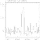
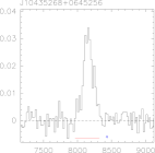
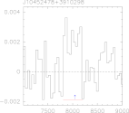
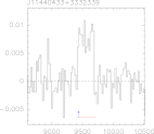
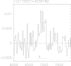
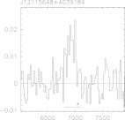
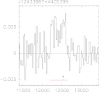
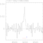
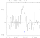
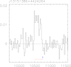
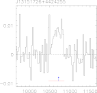
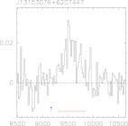
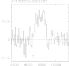
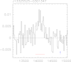
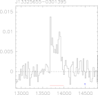
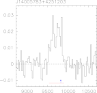
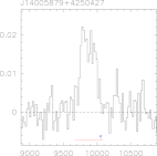
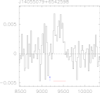
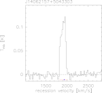
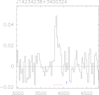
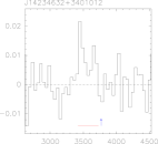
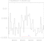
Figure 1: Continued.

     

       

     

     

   

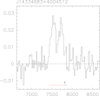
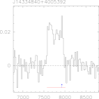
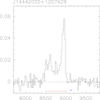
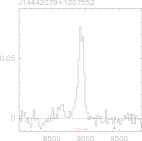
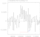
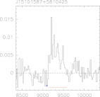
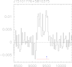
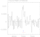
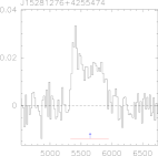
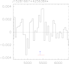
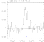
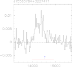
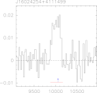
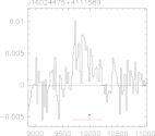
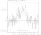
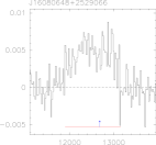
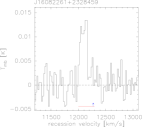
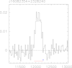
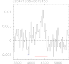
Figure 1: Continued

     

     

     

     

     

     

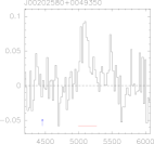
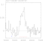
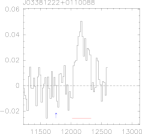
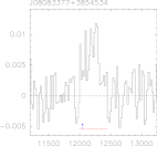
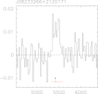
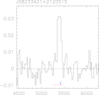
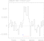
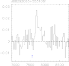
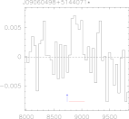
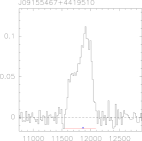
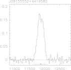
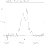
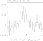
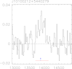
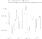
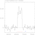
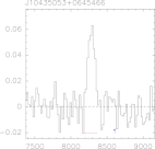
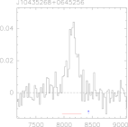
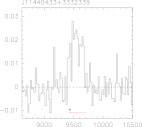
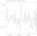
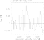
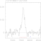
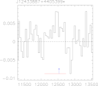
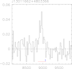
Figure 2: CO(2-1) spectra of the detected galaxies (including tentative detections). The velocity resolution is $\sim$ 20 km s^-1 for most spectra and $\sim$ 40 km s^-1 for some cases where a lower resolution was required to clearly see the line. The red line segment shows the zero-level linewidth of the CO line adopted for the determination of the velocity integrated intensity. The blue upright arrow indicated the optical heliocentric recession velocity. An asterisk next to the name indicates a tentative detection.

     

     

     

     

     

     

 

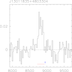
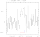
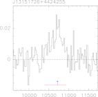
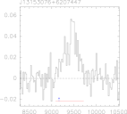
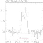
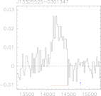
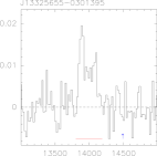
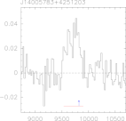
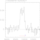
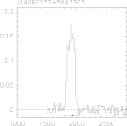
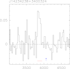
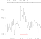
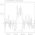
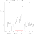
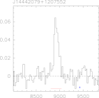
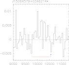
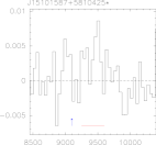
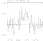
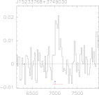
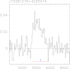
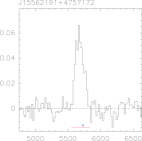
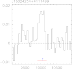
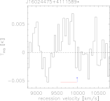
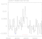
Figure 1: Continued.

This empirical aperture correction potentially could introduce a bias in our analysis. We therefore investigate in Figure 1 the distribution of $f_{{\rm aper}}$, separate for S+S pairs and S+E pairs. Two features are visible that are relevant for this question. Firstly, for most of the objects, the aperture correction is below 2 (91%, and 60% below 1.5) which means that possible errors introduced by this correction are small. Secondly, the distribution of $f_{{\rm aper}}$ for spirals in S+S and in S+E pairs is very similar and no features indicating the presence of a bias are obvious.

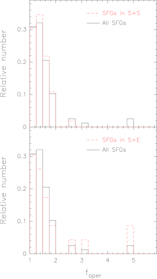
Figure 1: Histogram of the distribution of the aperture correction, $f_{{\rm aper}}$, for the different subsamples (red dashed line) compared to the full sample (full black line).

Table 2: Molecular gas mass

Galaxy name	Distance	log($M_{{\rm H}_{2}}$)	$f_{{\rm aper}}$
	[Mpc]	[$M_{\odot}$]
J00202580+0049350	64.4	9.44	2.63
J01183417-0013416	200.9	10.10	1.22
J01183556-0013594	201.7	9.71	1.29
J02110638-0039191	77.0	9.52	1.92
J03381222+0110088	172.9	9.80	1.38
….	….	….	….

3.3 Dust emission, SFR and stellar mass

All objects in our sample were imaged with the Herschel instruments PACS & SPIRE (Cao et al. 2016). These authors fitted the dust SED with the model of Draine et al. (2007) and derived the total IR luminosity, $L_{\rm IR}$, as well as the dust mass from it. They calculated the SFR from $L_{\rm IR}$ using the expression given in Kennicutt (1998), adapted to a Kroupa IMF, as SFR ($M_{\odot}$yr${}^{-1})=2.2\times 10^{-10}$ ($L_{\rm IR}$/$L_{\odot}$). This derivation of the SFR misses the contribution from unobscured UV radiation, which is on the order of 20% for KPAIR galaxies (Yuan et al. 2012). It can also be affected by the contribution of old stars to the dust heating which is about 30% for spiral galaxies (Buat & Xu 1996) and even lower ($0.17\pm 0.11$, Buat et al. 2011) for massive, actively star-forming galaxies. Thus, both affects are not expected to be severe for our actively star-forming sample. In addition, since we use the same formalism for both the H-KPAIR and the AMIGA control sample, these possible biases are not expected to affect the results involving the SFR.

The stellar mass was calculated from the 2MASS K_s-band luminosity as $M_{{\rm*}}$($M_{\odot}$) = 0.54 $L_{\rm K}$/$L_{\odot,\rm K}$ (Xu et al. 2012). The near-infrared K_s band luminosity, mainly from old stars that dominate the stellar mass, is insensitive to dust extinction and star formation (Bell & de Jong 2001). The calibration for the conversion from $L_{\rm K}$ to $M_{{\rm*}}$ was derived from a comparison between $L_{\rm K}$and $M_{{\rm*}}$ for normal galaxies in Kauffmann et al. (2013). We use the data provided by Cao et al. (2016), in particular the 70 $\mu$m  PACS flux, SFR, dust and stellar masses.

In addition, we derived the central 70 $\mu$m  and K_s band fluxes within the IRAM CO(1-0) beam directly from the corresponding images in order to locally compare the SFR and stellar mass with the measured molecular gas mass in the center of the galaxies, $M_{{\rm H_{2},center}}$. To achieve this, we multiplied the 70 $\mu$m image ($Im_{\rm 70\mu m}(x,y)$) and the K_s image ($Im_{\rm Ks}(x,y)$) with the IRAM beam pattern (approximated as a normalized Gaussian beam) placed at the position where the CO beam was pointed during the observations ($x_{0},y_{0})$:

$$Im_{\rm 70\mu m,beam}(x,y)=Im_{\rm 70\mu m}(x,y)\cdot\exp{\left(\frac{(x-x_{0})^{2}+(y-y_{0})^{2})}{2\sigma^{2}}\right)}$$ (5)

A corresponding expression is used for the K_s band image. The Gaussian standard deviation $\sigma$ is related to the FWHM as $\sigma$ = FWHM/$(2\sqrt{2\ln(2)})$ = FWHM/2.35. For the K_s band image we use the FWHM of the IRAM 30m CO(1-0) beam, FWHM = FWHM(IRAM) = 21.34″(1+z). For the 70 $\mu$m PACS image we use a slightly smaller value, FWHM =$\sqrt{\rm FWHM(IRAM)^{2}-FWHM(PACS)^{2}}$, in order to take into account that the 70 $\mu$m image is already convolved to the PACS resolution, FWHM(PACS)$\sim$ 6″. From the resulting maps $Im_{\rm 70\mu m,beam}(x,y)$ and $Im_{\rm Ks,beam}(x,y)$ we then measured the total 70 $\mu$m flux, $S_{\rm 70\mu m,center}$, and K_s flux, $S_{\rm Ks,center}$. We derived the central stellar mass within the IRAM beam from $S_{\rm Ks,center}$ with the same relation as for the total stellar mass (see above). For the central SFR we assumed that it is well traced by the 70 $\mu$m emission and derived it as ${\rm SFR_{center}}={\rm SFR}\cdot S_{\rm 70\mu m,center}/S_{\rm 70\mu m}$ where SFR and $S_{\rm 70\mu m}$ are the total SFR and 70 $\mu$m flux from Cao et al. (2016), respectively.

3.4 Atomic gas

We use the data for the atomic hydrogen (HI) data for 70 galaxy pairs (34 S+S pairs and 36 S+E pairs) from the H-KPAIR sample, from Zuo et al. (2018). These authors observed 58 pairs with the Green Bank Telescope (GBT) and retrieved the data for an additional 12 pairs from the literature, giving a total of 70 pairs with HI data. We have CO data for 38 of these pairs.

4 Results

In the following section, we mainly study the relations between molecular gas mass, atomic gas mass, dust mass, stellar mass and SFR. The main goal is to search for differences between spiral galaxies in S+S and in S+E pairs, for trends with the stellar mass, and to investigate the influence of the stage of the merger process by distinguishing galaxies classified as not showing any merger signs (labeled ”JUS”) from galaxies with interactions signs (labeled ”INT”) and pairs in the process of merging (labeled ”MER”). Following Cao et al. (2016), we exclude from our sample galaxies with a low sSFR $<-11.3$ yr^-1 (7 objects, only 1 detection in CO(1-0)) which belong to the red sequence and are thus not actively star-forming galaxies.

Since the beam of the GBT (9 ′ for HI) is too large to separate the emission from the individual galaxies, the analysis taking into account HI data is done for each pair as a whole. For S+S pairs we sum the values for the SFR, stellar mass, dust mass and molecular gas for both components. We then divide these values, as well as the HI mass, by two in order to obtain values typical for one galaxy. If only one member of a pair is observed in CO (2 cases), we flag the total molecular gas mass and the total gas mass as a lower limit. For S+E pairs we assume, following Zuo et al. (2018), that the atomic gas is mostly associated to the spiral component. Zuo et al. (2018), tested this assumption using the gas mass derived from the dust mass (Cao et al. 2016) and found that the mean gas mass in elliptical is only about 10% of the total mass in a S+E pair. We thus make a 10% correction and assume that $M_{\rm HI}$ of the spiral component in S+E pairs is 90% of the $M_{\rm HI}$ observed in the pair. The other variables, $M_{{\rm H}_{2}}$, $M_{{\rm*}}$, SFR and $M_{{\rm dust}}$ are taken for the spiral component only.

We list the mean and median values for different ratios, separated for the different groups, in Table LABEL:tab:means. In this table, we present the values for the entire galaxies (or pairs). As a check, we also examined all relations involving $M_{{\rm H}_{2}}$, $M_{{\rm*}}$ and SFR for the central values within the IRAM beam. We obtained very similar results, with the mean values agreeing within the errors. This supports the robustness of our conclusions,

4.1 Comparison sample

In order to search for differences between our merger sample and non-interacting galaxies, we need to compare our results to a suitable comparison sample. The comparison sample used in Cao et al. (2016) which was selected from the SDSS and matched to the HKPAIR sample does not include data for the molecular gas and can therefore only be used for a comparison of the SFR or $M_{{\rm dust}}$, which is a good indicator for the total gas mass (e.g., Eales et al. 2012; Corbelli et al. 2012).

Different catalogues of non-interacting galaxies containing CO, HI, SFR and $M_{{\rm*}}$ exist in the literature, e.g. the AMIGA sample of isolated galaxies (Verdes-Montenegro et al. 2005; Lisenfeld et al. 2011), the COLDGASS sample of mass-selected nearby galaxies (Saintonge et al. 2011a, b) and a catalogue of the ISM of normal galaxies (Bettoni et al. 2003). Here, we use the AMIGA and the COLD GASS sample for comparison because the CO observations for both samples have been taken with the IRAM 30m telescope and have been processed in a similar way as for our interacting sample. We present the relevant mean and median values in Table 3. We adapt all values to the Kroupa IMF, the Galactic $\alpha_{\rm CO}$  and do not include helium and heavy metals in the gas masses, and we limit the objects to those with sSFR $>-11.3$ yr^-1, as in our pair sample.

The AMIGA sample consisting of 1050 local isolated galaxies (Verdes-Montenegro et al. 2005). Out of this sample, a volume-limited (recession velocities between 1500 and 5000 km s^-1) subsample of 173 object possess CO data and their molecular gas properties were analyzed in Lisenfeld et al. (2011). The CO data were observed, as in the present paper, for the central position of the galaxy and the total molecular mass was calculated with the same extrapolation procedure as in the present paper. In Lisenfeld et al. (2011) the K-band luminosities, $L_{\rm K}$, are presented and we use them to calculate the stellar mass in the same way as here (see Sect. 3.3). Also the SFR is calculated in a very similar way as here from the total FIR luminosity based on IRAS data, $L_{\rm IR}$, following the expression from Kennicutt (1998). The AMIGA sample comprises a stellar mass range of (log($M_{{\rm*}}$) $\sim$ 9-11 which extends to lower masses than our sample. Therefore, we recalculated all mean and median values restricting the sample to high-mass spirals ($M_{{\rm*}}$$>10^{10}$ $M_{\odot}$), and using the Kaplan-Meier estimator to take upper limits into account.

The COLD GASS galaxy sample (Saintonge et al. 2011a, b) is a mass-selected ($M_{{\rm*}}$$>10^{10}$ $M_{\odot}$) local sample of $\sim$ 350 galaxies. The HI fluxes were obtained from the GASS survey (Catinella et al. 2018). The COLD GASS sample matches the HKPAIR sample in stellar mass (log($M_{{\rm*}}$) $\sim$ 10-11.4). The CO (1-0) was observed with the IRAM 30m telescope for the central position. In order to obtain the total CO flux, an aperture correction was derived by the authors based on CO maps of nearby spiral galaxies (Kuno et al. 2007) for which the impact of the observation with the IRAM beam was simulated for different redshifts. In this way, the flux that would be measured by a 22″ Gaussian beam ($S_{\rm CO-beam}$) was calculated and compared to the total flux of the maps, $S_{\rm tot}$. The dependence of the aperture correction factor $S_{\rm tot}/S_{\rm CO-beam}$ on the optical radius, $d_{\rm 25}$, was fitted and provided an aperture correction as a function of $d_{\rm 25}$ (see eq. 2 in Saintonge et al. 2011a). For galaxies with $d_{\rm 25}$$\geq$ 40″ they improved the scatter in the relation between the aperture correction factor and $d_{\rm 25}$ by performing an offcenter pointing along the major axis and used an empirical relation based on the ratio of the offcenter and central CO fluxes (see eq. 3 in Saintonge et al. 2011a). The stellar mass and the SFR were calculated from optical/UV spectral energy distribution (SED) based on a Chabrier IMF, which is very similar to the Kroupa IMF used in the present paper. In order to match the COLD GASS sample to ours, we furthermore made two restrictions: (i) We selected late-type galaxies based on the concentration index, C (the ratio of the r-band Petrosian radii encompassing 90% and 50% of the flux, $C=r_{90,r}/r_{50,r}$). We selected those galaxies with $C>2.85$ corresponding to galaxies with morphological types of Sa or later (Yamauchi et al. 2005). (ii) We excluded those galaxies that were found to be in pairs by Pan et al. (2018).

The results for the two comparison samples are reasonably consistent. The mean values have differences of less than $2\sigma$ except for the molecular gas fraction where the AMIGA sample has a mean value which is $0.22\pm 0.06$ dex lower than that of the COLDGASS sample. The reason for this difference is not completely clear. The AMIGA sample was selected with strict isolation criteria and has a low molecular gas content (Lisenfeld et al. 2011) and a low SFR (Lisenfeld et al. 2007) compared to other samples. However, if this were the reason for the difference with COLDGASS, we would expect not only a difference in $M_{{\rm H}_{2}}$/$M_{{\rm*}}$ but a similar difference in $M_{{\rm H}_{2}}$/$M_{\rm HI}$ which is not the case. In the following, we use the AMIGA sample for quantitative comparisons, but we note that all the conclusions are also valid compared to the COLDGASS sample.

Table 3: Mean and median values of the comparison samples

Parameter	AMIGA	ColdGASS	Cao et al. (2016)
	mean	mean	mean
	median	median	median
	$n/n_{\rm up}$	$n/n_{\rm up}$	$n$
log($M_{{\rm H}_{2}}$/$M_{\rm HI}$)	-0.63$\pm$0.06	-0.49$\pm$0.05
	-0.58	-0.46
	76/12	81/10
log($M_{{\rm H}_{2}}$/$M_{{\rm*}}$)	-1.48$\pm$0.05	-1.26$\pm$0.04
	-1.35	-1.20
	78/14	168/15
log($M_{{\rm gas}}$/$M_{{\rm*}}$)	-0.76$\pm$0.05	-0.82$\pm$0.04
	-0.71	-0.80
	77/13	81/10
log(SFE)	-9.07$\pm$0.05	-8.97$\pm$0.04
	-9.13	-8.98
	62/7	168/15
log(SFEgas)	-9.73$\pm$0.05	-9.63$\pm$0.07	-9.81$\pm$ 0.05
	-9.79	-9.66	–
	61/6	81/10	132/0

4.2 CO line ratio

In our sample we have 53 objects for which measurements for both $I_{\rm CO(1-0)}$ and $I_{\rm CO(2-1)}$ are available and which allow us to derived their line ratios. We show the relation between both lines in Fig. 2. We derive (taking upper limits in $I_{\rm CO(2-1)}$ into account) a mean value of $R_{\rm 21}$=$I_{\rm CO(2-1)}$/$I_{\rm CO(1-0)}$= 1.5 $\pm$ 0.1. If we only take objects with detections in both $I_{\rm CO(1-0)}$ and $I_{\rm CO(2-1)}$ into account (42 galaxies) the mean value is $R_{\rm 21}$= 1.7 $\pm$ 0.1. Both values are not aperture corrected.

To interpret $R_{\rm 21}$ one has to consider, apart from the excitation temperature of the gas, two main parameters: the source size relative to the beam and the opacity of the molecular gas. For optically thick, thermalized emission with a point-like distribution we expect a ratio $R_{\rm 21}$ = $\Theta^{2}_{\rm B(CO10)}/\Theta^{2}_{\rm B(CO21)}=4$ (with $\Theta_{\rm B}$ being the FWHM of the beams). On the other hand, for a source that is more extended than the beams we expect $R_{\rm 21}$$\sim 0.6-1$ for optically thick gas in thermal equilibrium, where $R_{\rm 21}$  depends on the temperature of the gas, and $R_{\rm 21}$$>1$ for optically thin gas.

We derive for our sample a mean $R_{\rm 21}$$>1$ which could be interpreted as a source extension smaller than at least the CO(1-0) beam or an extended source and optically thin emission. Based on our data alone, we cannot distinguish between these two cases. We can, however, consider results for spatially resolved observations from the literature which allows to derive the emission of CO(1-0) and CO(2-1) from the same area so that the source-to-beam size is irrelevant.

Matched aperture observations of CO(1-0) and CO(2-1) give line ratios of $R_{\rm 21}$$=0.89\pm 0.6$ (Braine & Combes 1993, for a small sample of nearby spiral galaxies), $R_{\rm 21}$$\sim 0.8$ (Leroy et al. 2009, for the SINGS sample), and $R_{\rm 21}$$\sim 0.6-0.9$ (Casasola et al. 2015, for 4 low-luminosity AGNs from the NUGA survey). $R_{\rm 21}$$\sim 0.8$ is consistent with optically thick gas with an excitation temperature of $\sim$10 K (Leroy et al. 2009). It is therefore very likely that a similar situation holds in our sample so that $R_{\rm 21}$$>1$ can be interpreted as optically thick, thermalized gas which a spatial extension smaller than (at least) the CO(1-0) beam.

Based on these assumptions, we can quantify the relation between $R_{\rm 21}$ and the source size in a simple model. The relation between the velocity integrated intensity and the intrinsic source brightness temperature, $T_{\rm B}$, is (Solomon et al. 1997):

$$I_{\rm CO}\Omega_{\rm S*B}(1+z)=T_{\rm B}\triangle V\Omega_{\rm S},$$ (6)

where $\Omega_{S*B}$ is the solid angle of the source convolved with the beam. Adopting for simplicity a source with a Gaussian distribution and neglecting the redshift dependence we obtain:

$$I_{CO}=T_{B}\triangle V\frac{\Omega_{S}}{\Omega_{S*B}}=T_{B}\triangle V\frac{\Theta^{2}_{S}}{\Theta^{2}_{B}+\Theta^{2}_{S}},$$ (7)

where $\Theta_{S}$ is the FWHM of the source. With these simplifications, and furthermore assuming that the intrinsic brightness temperature $T_{\rm B}$ is the same for both lines we can describe the line ratio as

$$R_{\rm 21}=\frac{I_{\rm CO(2-1)}}{I_{\rm CO(1-0)}}=\frac{\Theta^{2}_{\rm B(CO10)}+\Theta^{2}_{\rm S}}{\Theta^{2}_{\rm B(CO21)}+\Theta^{2}_{\rm S}}.$$ (8)

For point-like source ($\Theta^{2}_{\rm S}\ll\Theta^{2}_{\rm B}$) the line ratio is $R=4$.

Again adopting Gaussian distributions for both the source and the beam we can derive the aperture correction as a function of beam and source sizes:

$$f_{\rm aper}=\frac{S_{\rm CO,tot}}{S_{\rm CO,center}}=\frac{\Theta^{2}_{S}}{\Theta^{2}_{\rm B(CO10)}}+1,$$ (9)

where $S_{\rm CO,tot}$ is the total flux of the source and ${S_{\rm CO,center}}$ is the flux observed within the Gaussian CO(1-0) beam. Together, eq. 8 and 9 yield a relation between the aperture correction and the line ratio, both derived within the simplifying assumptions made here. We show the resulting relation in Fig.  2. It described the observed line ratios reasonably well, supporting the correctness of the aperture relation that we use here.

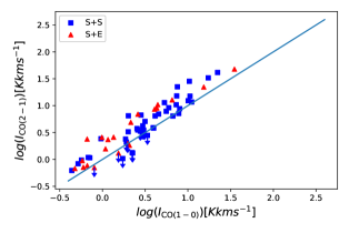
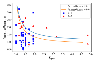
Figure 2: $I_{\rm CO(2-1)}$ as a function of $I_{\rm CO(1-0)}$(top panel). The line indicates unity. In the lower panel we show the line ratio as a function of the aperture correction, $f_{{\rm aper}}$, together with the prediction of a simple model assuming a Gaussian source and beam size. The model results are shown for two values of the ratio of the intrinsic source brightness temperatures.

4.3 Molecular gas, atomic gas and stellar mass

Figure 3 shows the molecular and atomic gas mass of the pairs. There is only a weak correlation (the Spearman’s rank correlation coeficient is 0.27 and the significance is 0.096). The ratio between molecular and atomic gas mass is shown in Figure 4 as a function of stellar mass. The mean molecular-to-atomic gas mass ratio (see Table LABEL:tab:means) is significantly higher than the value for the AMIGA comparison sample (by $0.38\pm 0.12$ dex). When inspecting the mean values of different subsamples (see Table LABEL:tab:means), we find the largest and most significant differences between galaxies with and without morphological signs of interaction. Whereas the JUS sample has a mean log($M_{{\rm H}_{2}}$/$M_{\rm HI}$) compatible within the errors with the comparison samples, the INT+MER galaxies have a value which is higher by $0.69\pm 0.16$. This difference is more significant for S+S galaxies than for S+E galaxies although the number of galaxies in the corresponding subsamples are very low. There is a difference of $0.55\pm 0.18$ dex in log($M_{{\rm H}_{2}}$/$M_{\rm HI}$) between S+S and S+E pairs, with the value for S+E pair being compatible with the comparison sample and that for S+S pairs being higher. As for subsamples with different stellar mass, there is no difference for the entire sample. Only for the subsample of S+S pairs there is a difference of $0.51\pm 0.16$ dex between low stellar mass (log($M_{{\rm*}}$) $<10.7$ $M_{\odot}$) and high stellar mass (log($M_{{\rm*}}$) $>10.7$ $M_{\odot}$) but the subsamples contain a low number of galaxies.

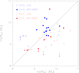
Figure 3: Molecular gas mass vs. atomic gas mass of galaxy pairs. The values for $M_{\rm HI}$ and $M_{{\rm H}_{2}}$ are divided by 2 for the S+S pair. To guide the eye, we include the line of unity ($M_{\rm HI}$= $M_{{\rm H}_{2}}$, black line).

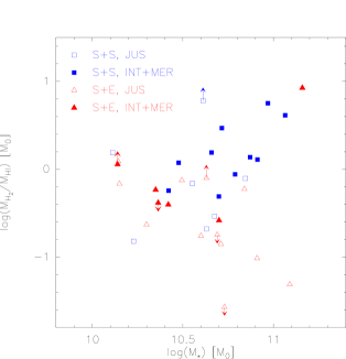
Figure 4: The ratio between molecular gas mass and atomic gas mass of galaxy pairs as a function of stellar mass. The values for $M_{\rm HI}$ and $M_{{\rm H}_{2}}$ are divided by 2 for the S+S pair.

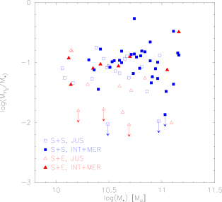
Figure 5: Molecular gas mass fraction (= $M_{{\rm H}_{2}}$/$M_{{\rm*}}$) vs. stellar mass.

Figure 5 shows the molecular gas fraction (defined as $M_{{\rm H}_{2}}$/$M_{{\rm*}}$) as a function of stellar mass. The mean logarithmic molecular gas fraction is above the values found for the comparison sample by $0.34\pm 0.07$ dex for the AMIGA and by $0.12\pm 0.06$ for the COLDGASS sample. Also here, there is a large and significant difference ($0.32\pm 0.9$ dex) between the mean values of the JUS and INT+MER sample. This difference is also present when considering the S+S and S+E galaxies separately. The molecular gas fracion is also smaller for star-forming galaxies in S+E galaxies compared to S+S galaxies, with a difference of difference is $0.21\pm 0.11$ dex (1.9$\sigma$). There is no trend with the stellar mass.

The total gas mass fraction ($M_{{\rm gas}}$/$M_{{\rm*}}$= ($M_{{\rm H}_{2}}$+$M_{\rm HI}$)/$M_{{\rm*}}$), shown in Figure 6, does not show any trends with stellar mass, pair type (S+S or S+E) nor morphological feature of interaction.

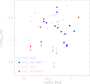
Figure 6: Total gas mass fraction (($M_{{\rm H}_{2}}$+$M_{\rm HI}$)/$M_{{\rm*}}$) vs. stellar mass of galaxy pairs. The values for $M_{{\rm dust}}$ and ($M_{\rm HI}$+$M_{{\rm H}_{2}}$) are devided by 2 for the S+S pair.

4.4 Molecular, atomic and dust mass

The molecular gas mass shows a good correlation with the dust mass from Cao et al. (2016) (Figure 7). The Spearman’s rank correlation coeficient is 0.73 and the significance is $8.4\times 10^{-12}$. The correlation is even tighter with the total gas mass (Figure 8) (Spearman’s rank correlation coeficient of 0.84 and significance $3.7\times 10^{-9}$).

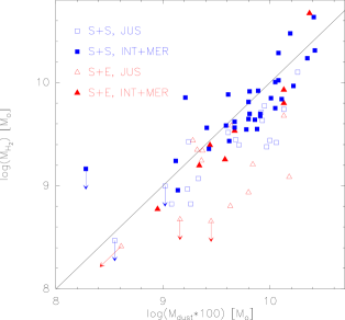
Figure 7: Molecular gas mass vs. $100\times$ dust mass. The line shows unity.

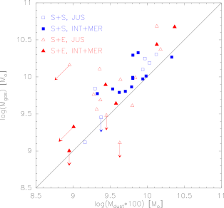
Figure 8: Total gas (molecular + atomic) mass vs. total $100\times$ dust mass of galaxy pairs. The values for $M_{{\rm dust}}$ and ($M_{\rm HI}$+$M_{{\rm H}_{2}}$) are devided by 2 for the S+S pair. The line shows unity.

Figure 9 shows the ratio between the total gas mass and the dust mass as a function of stellar mass. The mean value is $138$ with an error of 12 %. No trend with the stellar mass is visible, nor a significant difference between S+S or S+E pairs or as a function of interaction morphology. The mean value is very close to the mean value for nearby galaxies ($M_{{\rm gas}}$/$M_{{\rm dust}}$= 137, Draine et al. 2007, their Tab. 2), with values ranging between $\sim 100$ and 400. The relatively constant gas-to-dust mass ratio confirms the correctness of the analysis of Cao et al. (2016) who used the dust mass as a gas mass tracer.

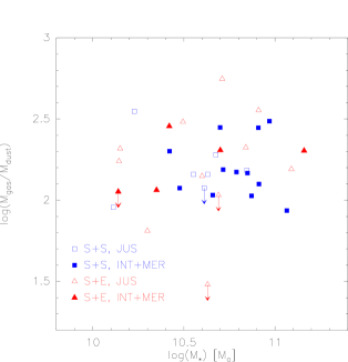
Figure 9: The gas-to-dust mass ratio vs stellar mass in galaxy pairs. The values for $M_{{\rm dust}}$, $M_{{\rm*}}$and ($M_{\rm HI}$+$M_{{\rm H}_{2}}$) are devided by 2 for the S+S pair.

4.5 Gas mass, stellar mass and star formation rate

Figure 10 shows the SFR as a function of $M_{{\rm H}_{2}}$. We also show the relation between SFR and $M_{{\rm H}_{2}}$ found for the AMIGA sample which is consistent with linearity (Lisenfeld et al. 2011), together with the standard deviation. The galaxies in S+S pairs follow this relation reasonably well, whereas spirals in S+E pairs lie below.

Figure 11 shows the relation between the SFE, defined as the ratio between SFR and molecular gas mass (SFE = SFR/$M_{{\rm H}_{2}}$) and the stellar mass. The value of log(SFE) for spirals in S+E pairs is below that of spirals in S+S pairs by $0.18\pm 0.06$ dex (see Table LABEL:tab:means).

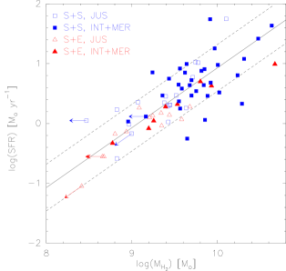
Figure 10: Star formation rate as a function of molecular gas mass. The lines are not a fit to the data, they show the mean value (full line) and dispersion (dashed lines) of the AMIGA comparison sample.

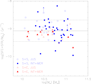
Figure 11: Star formation efficiency (= (SFR)/$M_{{\rm H}_{2}}$) vs stellar mass. The lines are not a fit to the data, they show the mean value (full line) and dispersion (dashed lines) of the AMIGA comparison sample.

Figure 12 shows the SFR as a function of the total (molecular + atomic) gas mass, and Figure 13 the ratio between the SFR and the gas mass (SFE_gas= SFR/$M_{{\rm gas}}$). The difference between S+S and S+E spirals is even more pronounced than for the SFE; the value of log(SFE_gas) is higher by $0.42\pm 0.11$ dex for spirals in S+S compared to S+E pairs. Again, no trend with $M_{{\rm*}}$ or the interaction phase is found.

This difference in SFE_gas between S+S and S+E pairs is in agreement with the results of Cao et al. (2016) who studied the SFE_gas  using the dust mass as a tracer of the total gas mass for the H-KPAIR sample. They found that log(SFE_gas) is $0.3\pm 0.1$ higher for spirals in S+S pairs than for S+E pairs.

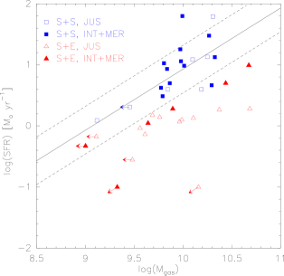
Figure 12: Star formation rate as a function of total (molecular+atomic) gas mass. To guide the eye, the lines are the same as in Fig. 10 and show the mean value (full line) and dispersion (dashed lines) of the AMIGA comparison sample.

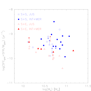
Figure 13: Star formation efficiency per total gas mass (SFE_gas= (SFR)/$M_{{\rm gas}}$) vs. stellar mass.

Table 4: Mean and median values of parameters for the total sample and subsamples. The X-factor was chosen to vary with the distance from the galaxy MS as described in Sect. 5.1. Not to be shown in the paper, just for our comparison.

	S+S	S+E	log($M_{{\rm*}}$)$<10.7$	log($M_{{\rm*}}$)$>10.7$	JUS	INT+MER	Total
	mean	mean	mean	mean	mean	mean	mean
	median	median	median	median	median	median	median
	n/nup	n/nup	n/nup	n/nup	n/nup	n/nup	n/nup
	-8.93$\pm$0.07	-9.18$\pm$0.04	-8.96$\pm$0.06	-9.04$\pm$0.10	-8.95$\pm$0.08	-9.02$\pm$0.08	-8.99$\pm$0.05
SFE	-8.91	-9.18	-8.98	-9.11	-9.07	-9.05	-9.05
	49/2	20/2	38/3	31/1	29/3	40/1	69/4
			-8.88$\pm$0.08	-8.98$\pm$0.11	-8.84$\pm$0.10	-8.97$\pm$0.09
SFE	–	–	-8.87	-9.01	-8.97	-8.91	–
S+S			24/1	25/1	17/1	32/1
			-9.14$\pm$0.03	-9.26$\pm$0.10	-9.16$\pm$0.06	-9.20$\pm$0.05
SFE	–	–	-9.11	-9.22	-9.11	-9.18	–
S+E			14/2	6/0	12/2	8/0
	-9.27$\pm$0.09	-9.74$\pm$0.07	-9.46$\pm$0.06	-9.49$\pm$0.14	-9.60$\pm$0.11	-9.33$\pm$0.10	-9.46$\pm$0.08
SFEgas	-9.29	-9.65	-9.47	-9.60	-9.64	-9.44	-9.47
	19/1	16/3	20/4	15/0	18/3	17/1	35/4
	–	–	-9.37$\pm$0.08	-9.18$\pm$0.16	-9.34$\pm$0.13	-9.25$\pm$0.12	–
SFEgas	–	–	-9.40	-9.19	-9.34	-9.29	–
S+S	–	–	10/1	9/0	7/1	12/0	–
	–	–	-9.60$\pm$0.06	-9.96$\pm$0.11	-9.81$\pm$0.09	-9.59$\pm$0.05	–
SFEgas	–	–	-9.63	-9.93	-9.76	-9.63	–
S+E	–	–	10/3	6/0	11/2	5/1	–
	-0.07$\pm$0.10	-0.51$\pm$0.15	-0.34$\pm$0.08	-0.18$\pm$0.17	-0.56$\pm$0.12	0.03$\pm$0.10	-0.27$\pm$0.10
$M_{{\rm H}_{2}}$/$M_{\rm HI}$	0.06	-0.55	-0.36	-0.13	-0.64	0.06	-0.16
	18/0	16/3	18/2	16/1	17/2	17/1	34/4
	–	–	-0.31$\pm$0.12	0.17$\pm$0.12	-0.43$\pm$0.14	0.11$\pm$0.10	–
$M_{{\rm H}_{2}}$/$M_{\rm HI}$	–	–	-0.32	0.08	-0.38	0.06	–
S+S	–	–	9/0	9/0	6/0	12/0	–
	–	–	-0.35$\pm$0.10	-0.62$\pm$0.28	-0.64$\pm$0.16	-0.17$\pm$0.24	–
$M_{{\rm H}_{2}}$/$M_{\rm HI}$	–	–	-0.36	-0.77	-0.68	-0.36	–
S+E	–	–	9/2	7/1	11/2	5/1	–
	-1.16$\pm$0.04	-1.31$\pm$0.09	-1.23$\pm$0.05	-1.18$\pm$0.07	-1.36$\pm$0.07	-1.09$\pm$0.04	-1.21$\pm$0.04
$M_{{\rm H}_{2}}$/$M_{{\rm*}}$	-1.15	-1.24	-1.15	-1.2	-1.28	-1.06	-1.17
	50/3	21/3	39/4	32/2	31/5	40/1	71/6
			-1.17$\pm$0.05	-1.15$\pm$0.07	-1.28$\pm$0.07	-1.09$\pm$0.05
$M_{{\rm H}_{2}}$/$M_{{\rm*}}$			-1.15	-1.18	-1.25	-1.06
S+S			24/1	26/2	18/2	32/1
			-1.32$\pm$0.11	-1.30$\pm$0.17	-1.48$\pm$0.12	-1.05$\pm$0.07
$M_{{\rm H}_{2}}$/$M_{{\rm*}}$			-1.1	-1.24	-1.39	-1.06
S+E			15/3	6/0	13/3	8/0
	-0.76$\pm$0.06	-0.79$\pm$0.10	-0.79$\pm$0.09	-0.76$\pm$0.07	-0.74$\pm$0.09	-0.79$\pm$0.06	-0.77$\pm$0.06
$M_{{\rm gas}}$/$M_{{\rm*}}$	-0.76	-0.67	-0.62	-0.84	-0.64	-0.84	-0.68
	19/1	18/5	21/5	16/1	19/4	18/2	37/6
	2.16$\pm$0.05	2.18$\pm$0.09	2.13$\pm$0.06	2.25$\pm$0.06	2.18$\pm$0.08	2.18$\pm$0.05	2.18$\pm$0.05
$M_{{\rm gas}}$/$M_{{\rm dust}}$	2.13	2.28	2.13	2.20	2.16	2.14	2.16
	19/1	16/3	20/4	15/0	18/3	17/1	35/4

4.6 “Holmberg effect”

”Holmberg effect” denotes usually any concordant behavior between the two components in galaxy pairs, after the discovery of Holmberg (1937) that binary galaxies tend to have similar morphologies and optical colors. Figure 14 shows the correlation between the molecular gas fraction ($M_{{\rm H}_{2}}$/$M_{{\rm*}}$) of the primary and secondary galaxies in S+S pairs. The Spearman’s rank correlation coeficient is 0.55 and the significance is $9.4\times 10^{-3}$. A similar ”Holmberg effect” has been found for the sSFR both by Xu et al. (2010), Cao et al. (2016) and, for a larger sample of 1899 galaxies, by Scudder et al. (2012).

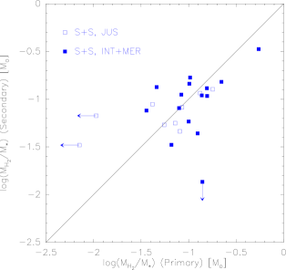
Figure 14: Molecular gas fraction of the secondary vs. primary galaxy in S+S pairs.

5 Discussion

5.1 Effect of a variable X-factor

We base our analysis on a constant $L^{\prime}_{\rm CO}$-to-$M_{{\rm H}_{2}}$factor $\alpha_{\rm CO}$. It is well accepted that $\alpha_{\rm CO}$ can vary in different types of galaxies, mainly due to its dependence on metallicity and star formation activity (see Bolatto et al. 2013, and references therein). It can be considerably higher for low-metallicity galaxies (below 12+log(O/H) $\sim$ 8.4, e.g., Leroy et al. 2011; Bolatto et al. 2013; Hunt et al. 2015) and lower by a factor of 3-10 in extreme starbursts as ULIRGS (Downes & Solomon 1998, 2003).

Our sample does not contain low-metallicity galaxies because all galaxies are relatively high mass ($>10^{10}$ $M_{\odot}$), and neither does it contain extreme starburst galaxies, so that we do not expect $\alpha_{\rm CO}$ to vary considerably among them. We can test whether we find any indications of a relation with the SF activity by comparing the gas-to-dust mass ratio to the specific SFR (Fig. 15). If the molecular gas mass is correctly calculated we expect no trend with the sSFR. If, on the other hand, $\alpha_{\rm CO}$  were decreasing with the SF activity we would expect to see an overestimate of $M_{{\rm H}_{2}}$  and thus an increase of the gas-to-dust mass ratio for increasing sSFR. This is not the case, even for those objects where the molecular gas is dominating the gas mass. At most, there might be a weak trend in the opposite direction (decreasing gas mass with sSFR).

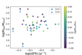
Figure 15: The gas-to-dust mass ratio as a function of the sSFR.

In spite of this lack of evidence for a variation of $\alpha_{\rm CO}$ in our sample, we test the effect of a possible variation following loosely the prescription proposed in Violino et al. (2018) and Sargent et al. (2014) who parametrized the variation of the conversion factor as:

$$\alpha_{\rm CO}=(1-f_{\rm SB})\alpha_{\rm CO,MS}+f_{\rm SB}\alpha_{\rm SB}$$ (10)

where $\alpha_{\rm CO,MS}$ is the conversion factor for galaxies lying on the galaxy main-sequence, $\alpha_{\rm CO,SB}$ is the value for extreme starburst galaxies and $f_{\rm SB}$ is the probability of a galaxy being in a starburst phase given its offset from the mean locus of the star-forming main sequence in the SFR-$M_{{\rm*}}$ plane. Violino et al. (2018) take into account a metallicity dependence of $\alpha_{\rm CO,MS}$, which we do not consider necessary for our high-mass sample, so that we take $\alpha_{\rm CO,MS}$ as the Galactic X-factor, $\alpha_{\rm CO,MS}$ = 3.2 $M_{\odot}$/(K km s^-1pc^-2) (Bolatto et al. 2013). We assume that $f_{\rm SB}$ varies linearly with the logarithmic distance of a galaxy from the galaxy main sequence, $\Delta_{\rm MS}$ = log(SFR) - log(SFR_MS). We use the MS location following the prescription by Saintonge et al. (2016, their eq. 5) because their sample encompasses roughly the same mass range as ours. We normalize $f_{\rm SB}$  by taking Arp 220 as a prototypical extreme starburst galaxy. Deriving the stellar mass from the K-band luminosity and the SFR from the far-infrared luminosity, we obtain $M_{{\rm*}}$= $1.4\times 10^{10}$ $M_{\odot}$ and SFR = 220 $M_{\odot}$ yr^-1 and find that Arp 220 lies a factor of 100 above the MS. We adopt $\alpha_{\rm CO,SB}$= 0.8 $M_{\odot}$/(K km s^-1pc^-2) (Downes & Solomon 1998). Together, this yields, for a linear relation between $f_{\rm SB}$ and $\Delta_{\rm MS}$, $f_{\rm SB}$= $\Delta_{\rm MS}/\log(100)=\Delta_{\rm MS}/2$. Finally, we assume that galaxies that fall below the MS have the Galactic $\alpha_{\rm CO}$  (i.e. $f_{\rm SB}$= 0).

We test all our results with this different prescription. The results obtained with this variable $\alpha_{\rm CO}$ are very similar to the ones with a constant, Galactic value. The differences are within the errors, and in particular all the differences and correlations that we found are also valid for a variable $\alpha_{\rm CO}$. Therefore we conclude that our results are robust with respect to reasonable uncertainties in the X-factor.

5.2 Variations of the SFE

Compared to AMIGA sample (Table 3), we find no enhancement in the SFE for the whole pair sample, nor for any of the subsamples (S+S and S+E. low mass and high mass, with and without interaction signs; see Table 4). It is controversial in the literature on whether paired galaxies have enhanced SFE compared to normal spirals. While Violino et al. (2018) and Pan et al. (2018) found weakly enhanced SFE ($\lesssim 2\times$), Solomon & Sage (1988), Combes et al. (1994), and Casasola et al. (2004) found no such enhancement.

We found a $\sim 3\sigma$ difference ($0.18\pm 0.6$) dex between the SFE of galaxies in S+S and in S+E pairs. Compared to the AMIGA sample the SFE in S+E is slightly decreased (by $0.13\pm 0.06$) dex, indicating a lower capacity of the molecular gas to form stars in S+E pairs. The difference with respect to the comparision sample is small and might be affected by systematic uncertainties, e.g. by the differences in the calculation of the SFR. The difference between the S+S and S+E subsample is more robust. It holds at a 3$\sigma$ level when using a variable $\alpha_{\rm CO}$ ($0.25\pm 0.08$) dex and when considering the central values for the molecular gas and SFR ($0.23\pm 0.7$) dex. It is unclear what the physical reason for this difference is. A possible reason could be hydrodynamical effects which are expect to be stronger in a S+S merger where the gas of both galaxies interacts compared to S+E mergers where the elliptical component has very little cold gas. However, we would then expect to see a noticeable difference mainly in the later stages of the interaction, whereas in our study we find no differences in the SFE between galaxies with and without interaction signs. Hwang et al. (2011) suggested that the hot gas halos around elliptical galaxies could be responsible for the differences in the SF activity found between S+S and S+E. However, it is unclear how the hot gas can directly affect the molecular gas without altering the total ($M_{\rm HI}$+ $M_{{\rm H}_{2}}$) gas content which we found equal for all subsample.

When considering the total gas, our results show significant enhancement in SFE_gas for S+S pairs ($0.42\pm 0.10$ dex), pairs with signs of interaction ($0.37\pm 0.10$ dex), and low mass pairs ($0.27\pm 0.08$ dex), but not for subsamples of S+E pairs, pairs without signs of interaction, and high mass pairs. Simulations (e.g. Renaud et al. 2014) have predicted enhanced SFE_gas in interacting galaxies, which is particularly strong during the final stage of a merger, but also during the early phase just after the first pericenter passage. Our results suggest that this scenario applies to S+S pairs, but not to S+E pairs. The mean SFE_gas of S+E subsample is consistent with that of control galaxies, and is lower than that of S+S by $0.42\pm 0.11$ dex. This result agrees well with that of (Cao et al. 2016) who found a difference between the mean SFE_gas of S+S and S+E pairs of $0.43\pm 0.13$ dex.

5.3 Variation of the molecular gas fraction

The molecular gas fraction ($M_{{\rm H}_{2}}$/$M_{{\rm*}}$) and molecular-to-atomic gas ratio ($M_{{\rm H}_{2}}$/$M_{\rm HI}$) are enhanced for INT+MER galaxies whereas for pairs at the beginning of the interaction (JUS) no enhancement is found. Significant enhancement is also present in S+S pairs but not in S+E pairs. The total gas content ($M_{{\rm gas}}$/$M_{{\rm*}}$), on the other hand, does not show any variation between the subsamples.

These results together give a consistent picture. From the total gas content in the galaxy, a considerable fraction is converted from atomic to molecular gas during the interaction. This conversion becomes stronger in a later stage, when morphological signatures are visible. We would then expect a similar trend for the sSFR, caused by the increase in the molecular gas fraction. Indeed, Cao et al. (2016) found a higher sSFR for INT+MER galaxies compared to JUS galaxies.

Our results are in general consistent with numerous previous observations that showed significant increase in the molecular gas content in interacting galaxies ((Braine & Combes 1993; Combes et al. 1994; Casasola et al. 2004; Violino et al. 2018; Pan et al. 2018). Our results, though, indicate that not all galaxies in close major-merger pairs have an enhanced molecular gas content, but only those in S+S pairs and pairs with interaction signs do.

With a statistically significant large and homogeneous sample of paired galaxies, confined to close major-merger pairs that have small separations and mass ratios, we pinpoint that the major enhancement occurs in the molecular-to-atomic gas ratio. This conclusion disagrees with Casasola et al. (2004). They investigated the molecular-to-atomic gas ratios of interacting galaxies and found that, for late types, these ratios are quite normal compared to the control sample. Given that both the interacting galaxy sample and the control sample of Casasola et al. (2004) were constructed heterogeneously and the multi-band data collected from the literature, their result most likely has larger uncertainties than ours, and, most importantly, their data does not allow a distinction between the pair type and interaction phase which we found to be crucial to find a difference in $M_{{\rm H}_{2}}$/$M_{\rm HI}$.

5.4 What drives the enhancement of the SFR in galaxy pairs?

Our results show that the increase of the SFR in close major-merger pairs is mainly driven by an enhancement in the molecular-to-HI gas ratio. The total gas content, on the other hand, is constant so that inflow or loss of gas can be excluded. The SFE is not significantly enhanced compared to control galaxies, while the increase in the SFE_gas can be explained by the enhancement of the molecular-to-HI gas ratio. Given that the enhancement is found only in pairs with signs of interaction and absent in pairs without, it is most likely triggered by the strong tidal torque after the first close encounter, which can compress the lower density HI gas into the higher density molecular gas. This scenario is different from that for (U)LIRGs which are in the final stage of coalescence. For (U)LIRGs, both the molecular gas content and SFE are strongly enhanced (Solomon & Sage 1988; Mirabel & Sanders 1989). It seems that in paired galaxies after the first close encounter, while the tidal torque compresses more gas into star forming giant molecular clouds (GMCs), the SFE of individual GMCs is still comparable to the standard value found in normal galaxies (Leroy et al. 2008). On the other hand, in (U)LIRGs such as Arp220, the GMCs in the central starburst are further compressed into a gas disk of very high density ($>10^{4}$ cm^-3), resulting in a much higher SFE (Scoville et al. 1997, 2017). Gao & Solomon (1999) found that, for infrared selected mergers, the $L_{\rm IR}$/$M_{{\rm H}_{2}}$ ratio increases nearly 10$\times$ when projected separation decreases from $\sim 30$ to $\sim 2$ kpc, consistent with a continuous transition of the SFE between close pairs and final stage mergers.

This change of SFE of molecular gas along the merger sequence may provide a new and important constraint to simulations of galaxy mergers. Currently no simulation has separated molecular gas from the atomic gas. An indirect inference may be drawn from the results of Renaud et al. (2014), who carried out parsec-resolution simulations with comprehensive treatment of turbulence and shocks. In their Fig. 2, they presented predictions of gas density Probability Distribution Functions (PDFs) of different merger epochs, with the $t=35$ Myr epoch corresponding to the starburst after the first close encounter and the $t=170$ Myr epoch to the starburst in the final coalescence. For both epochs, strong enhancements are found both in the ratio between densities of $\sim 100$ cm^-3 and $\sim 1$ cm^-3, which corresponds roughly to the molecular-to-atomic gas ratio, and in the ratio between densities of $\sim 10^{4}$ cm^-3 and $\sim 100$ cm^-3. The mass of dense gas of $\sim 10^{4}$ cm^-3 is linearly correlated to SFR (Gao & Solomon 2004), therefore the enhancement in the ratio between densities of $\sim 10^{4}$ cm^-3 and $\sim 100$ cm^-3 indicates an SFE enhancement both in the epoch after the first close encounter and in the final coalescence stage. This seems not fully consistent with our result which does not show strong SFE enhancement in paired galaxies.

We found differences in the SFE, SFE_gas and $M_{{\rm H}_{2}}$/$M_{\rm HI}$ between S+S and S+E subsamples. In particular the mean $M_{{\rm H}_{2}}$/$M_{\rm HI}$ ratio of the S+E is $0.55\pm 0.18$ dex lower than that of S+S (Table 4), and is consistent with those of the control samples (Table 3). The difference is caused by two factors: (1) only 31% (5/16) of star-forming galaxies in S+E show signs of interaction while 67% (12/18) of those in S+S do; (2) the mean $M_{{\rm H}_{2}}$/$M_{\rm HI}$ ratio of star-forming galaxies in S+E pairs without interaction signs is $0.35\pm 0.22$ dex lower than that of their counterparts in S+S. The first factor might be explained by the stabilizing effect that bulges can have during interaction, if star-forming galaxies in S+E are more likely to be earlier Hubble types with larger bulges compared to their counterparts in S+S, which is indeed expected according to the Holmberg effect (Holmberg 1958; Hernández-Toledo & Puerari 2001). Simulations have shown that large bulges can suppress the tidal effects during and after close encounters (Mihos & Hernquist 1996; Di Matteo et al. 2008; Cox et al. 2008), making it more difficult for conspicuous tidal features to form. Interestingly, star-forming galaxies in S+E pairs with interaction signs show an enhancement of $0.55\pm 0.30$ dex in $M_{H_{2}}/M_{HI}$ ratio compared to those in S+E pairs without interaction signs, suggesting that HI gas can also be compressed to molecular gas in S+E pairs when the tidal effects are sufficiently strong (indicated by interaction signs), similar to what is happening in S+S pairs with interaction signs. The factor (2), though with a low significance (1.6$\sigma$), might indicate that the progenitors of star-forming galaxies in S+E have lower $M_{{\rm H}_{2}}$/$M_{\rm HI}$ than those in S+S. Alternatively, the formation of the molecular gas due to tidal forces might have started early in the interaction and preferentially in the bulge-less S+S systems. x

6 Conclusions and summary

We presented new CO data for a sample of K_s-band selected local ($z<0.06$), close (projected separation $\lesssim 20\,h^{-1}$ kpc), major (mass ratio $\leq 2.5$) merger pairs which allows us to calculate the molecular gas mass. These data, together with a large set of ancillary data, allows us to study the molecular gas fraction, $M_{{\rm H}_{2}}$/$M_{{\rm*}}$, the molecular-to-atomic gas mass ratio, $M_{{\rm H}_{2}}$/$M_{\rm HI}$, SFE = SFR/$M_{{\rm H}_{2}}$, and SFE_gas= SFR/$M_{{\rm gas}}$ as a function of galaxy mass, interaction type (S+S or S+E pair) and interaction phase (undisturbed appearance ”JUS”, or with clear signs of tidal disturbance or merging ”INT+MER”). We compared the values of the merger sample to two comparison samples, AMIGA (Lisenfeld et al. 2011) and COLDGASS (Saintonge et al. 2011a, b). The main conclusions are:

1. We found no significant enhancement in SFE (=SFR/$M_{{\rm H}_{2}}$) for the whole pair sample, nor for any of the subsamples (S+S and S+E, low mass and high mass, with and without interaction signs). The SFE in star-forming galaxies in S+E pairs is $0.18\pm 0.6$ dex lower than in S+S pairs.

2. When considering the total gas, $M_{{\rm gas}}$= $M_{\rm HI}$+$M_{{\rm H}_{2}}$, our results show significant enhancement in SFE_gas for S+S pairs ($0.42\pm 0.09$ dex), pairs with signs of interaction ($0.37\pm 0.10$ dex), and low mass pairs ($0.27\pm 0.08$ dex), but not for subsamples of S+E pairs, pairs without signs of interaction, and high mass pairs.

3. We found an enhancement of $M_{{\rm H}_{2}}$/$M_{\rm HI}$  from JUS to INT+MER galaxies. The values of the JUS subsample are compatible with those of the control samples. A similar, albeit less significant, trend was found for $M_{{\rm H}_{2}}$/$M_{{\rm*}}$. This indicates that the amount of molecular gas enhances as the interaction proceeds.

4. We found differences in $M_{{\rm H}_{2}}$/$M_{\rm HI}$  and in $M_{{\rm H}_{2}}$/$M_{{\rm*}}$ between S+S and S+E subsamples. The mean $M_{{\rm H}_{2}}$/$M_{\rm HI}$  ratio and mean $M_{{\rm H}_{2}}$/$M_{{\rm*}}$ ratio of the S+E are $0.55\pm 0.18$ dex (2.5$\sigma$) and $0.21\pm 0.11$ dex (1.9$\sigma$) lower than those of the S+S, and are consistent with those of control samples.

Our results show that the star formation enhancement in close major-merger pairs is mainly driven by an accelerated conversion of atomic gas to molecular gas in pairs with interaction signs, likely triggered by the strong tidal effects after the first close encounter. Both the star formation and molecular gas content enhancements are significantly suppressed in star-forming galaxies in S+E pairs, probably due to the stabilizing effects of large bulges.

Appendix A Figures of spectra

     

     

     

     

     

     

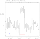
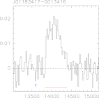
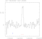
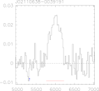
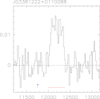
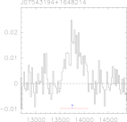
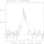
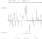
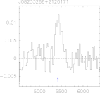
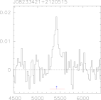
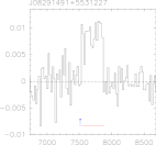
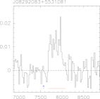
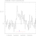
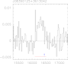
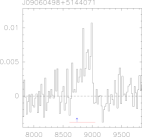
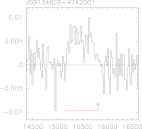
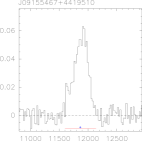
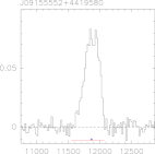
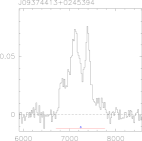
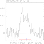
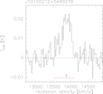
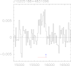
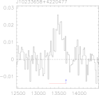
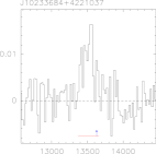
Figure 16: CO(1-0) spectra of the detected galaxies (including tentative detections). The velocity resolution is $\sim$ 20 km s^-1 for most spectra and $\sim$ 40 km s^-1 for some cases where a lower resolution was required to clearly see the line. The red line segment shows the zero-level linewidth of the CO line adopted for the determination of the velocity integrated intensity. The blue upright arrow indicated the optical heliocentric recession velocity. An asterisk next to the name indicates a tentative detection.