Chaos bound in Bershadsky-Polyakov theory

Abstract

We consider two dimensional conformal field theory (CFT) with large central charge $c$ in an excited state obtained by the insertion of an operator $\Phi$ with large dimension $\Delta_{\Phi}\sim O(c)$ at spatial infinities in the thermal state. We argue that correlation functions of light operators in such a state can be viewed as thermal correlators with a rescaled effective temperature. The effective temperature controls the growth of out-of-time order (OTO) correlators and results in a violation of the universal upper bound on the associated Lyapunov exponent when $\Delta_{\Phi}<0$ and the CFT is nonunitary. We present a specific realization of this situation in the holographic Chern-Simons formulation of a CFT with ${W}^{(2)}_{3}$ symmetry also known as the Bershadsky-Polyakov algebra. We examine the precise correspondence between the semiclassical (large-$c$) representations of this algebra and the Chern-Simons formulation, and infer that the holographic CFT possesses a discretuum of degenerate ground states with negative conformal dimension $\Delta_{\Phi}\,=\,-\frac{c}{8}$. Using the Wilson line prescription to compute entanglement entropy and OTO correlators in the holographic CFT undergoing a local quench, we find the Lyapunov exponent $\lambda_{L}=\frac{4\pi}{\beta}$, violating the universal chaos bound.

1 Introduction

It is well known that unitarity and causality in conformal field theories (CFTs) have been used to constrain the allowed spectra as well as to classify the allowed theories. For example, positivity of the norm in two dimensional CFTs constrains both the conformal dimensions of operators and the central charge to be positive. In fact, demanding positive eigenvalues of the Kac matrix, enables the classification of two dimensional CFTs with central charge $0<c<1$ and determination of the scaling dimensions of the primaries of these theories (see e.g. Ginsparg:1988ui ). Recently, constraints on other physically interesting observables have been shown to be related to unitarity and causality. For example, the fact that energy deposited in the detector of the conformal collider is positive Hofman:2008ar , or the average null energy condition, has been shown to be related to unitarity and causality Hartman:2015lfa ; Hofman:2016awc ; Hartman:2016lgu . The bound on the Lyapunov index which controls the growth of out-of-time ordered four-point functions, has also been argued to be related to unitarity and causality mss .

In two dimensions, it was was shown that unitarity, or more specifically, the positivity of the eigenvalues of the Kac matrix implies a bound on the spin-3 charge in a CFT with ${W}_{3}$ symmetry Afkhami-Jeddi:2017idc . In the large-$c$ limit the bound is given by,

$$9\left(\frac{\cal W}{c}\right)^{2}\leq\frac{64}{5}\left(\frac{\Delta}{c}\right)^{3}-\frac{2}{5}\left(\frac{\Delta}{c}\right)^{2}\,.$$ (1)

Here ${\cal W}$ is the spin-3 charge and $\Delta$ the conformal dimension of the primary carrying this charge. At the same time it was independently shown in David:2017eno that one can arrive at a bound on the higher spin charge, in a holographic large-$c$ CFT with $W_{3}$ symmetry, by demanding that the jump in entanglement entropy during a quantum quench by an operator carrying spin-3 charge is always real:

$$\sqrt{\frac{|{\cal W}|}{c}}<\frac{2\Delta}{c}\,.$$ (2)

It was also seen in David:2017eno that the bound (2) automatically ensures that the chaos bound on the Lyapunov index for the out-of-time ordered four-point function is obeyed . Remarkably, if we restrict ourselves to the unitarity bound (1), then (2) is always satisfied.

In this paper we would like to show that the chaos bound is also violated in certain holographic CFTs with (non-principal) W-symmetries but with spin $s\leq 2$ currents. The mechanism leading to violation of the bound is distinct from that demonstrated in $W_{N}$ theories with spin $s>2$ currents Afkhami-Jeddi:2017idc ; Perlmutter:2016pkf . We will see that the violation here is due to the existence of a nontrivial ground state (corresponding to an operator say, $\Phi$) with large, negative conformal dimension, $\Delta_{\Phi}<0$ and $|\Delta_{\Phi}|\sim O(c)$. To understand this we consider the setup shown in figure 1.

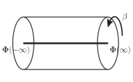
Figure 1: CFT at finite temperature $\beta^{-1}$ with heavy operators at spatial infinity.

Here we consider a conformal field theory at large central charge $c$ on an infinite line and at finite temperature $\beta^{-1}$. At the spatial infinities we insert an operator of conformal weights $(\Delta_{\Phi},\Delta_{\Phi})$ such that $|\Delta_{\Phi}|\sim O(c)$. The more familiar situation in the literature is when such an operator is inserted at temporal infinities on a cylinder of radius $2\pi$ as shown in figure 2. In this situation the vacuum energy of the cylinder is shifted from its usual conformal value (summing over both holomorphic and antiholomorphic sectors),

$${\cal E}\,+\,\bar{\cal E}\,=\,-\frac{c}{12}\,\to\,-\frac{c}{12}\left(1-\frac{24\Delta_{\Phi}}{c}\right)\,.$$ (3)

Furthermore, the analysis of Asplund:2014coa ; Fitzpatrick:2015zha shows that correlators of light operators inserted in the vacuum shown in figure 2 can be reproduced by considering the transformation to the plane

$$z\,=\,e^{-i\alpha\tilde{w}},\qquad\alpha=\sqrt{1-\frac{24\Delta_{\Phi}}{c}}\,.$$ (4)

Here $z$ is the coordinate in the plane and $\tilde{w}$ is the coordinate on the cylinder. It is easy to see the vacuum energy (3) follows from the Schwarzian of the above transformation. We thus see that the cylinder acquires a deficit angle $2\pi(1-\alpha)$. Holographically, this vacuum is dual to a conical defect created by a particle of mass $m=(\Delta_{\Phi}+\bar{\Delta}_{\Phi})/R$ where $R$ is the radius of AdS₃. The thermal state described in figure 1, though not very familiar, can be thought of as a Wick rotation of that in figure 2.

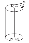
Figure 2: CFT on a cylinder with heavy operators at temporal infinity

The presence of the operator $\Phi$ shifts the energy density of the thermal state,

$${\cal E}\,+\,\bar{\cal E}\,=\,\frac{c\pi^{2}}{3\beta^{2}}\,\rightarrow\,\frac{c\pi^{2}}{3\beta^{2}}\left(1-\frac{24\Delta_{\Phi}}{c}\right)\,.$$ (5)

Note that we can obtain (3) from (5) by the replacement $\beta\rightarrow 2i\pi$. We show that correlators of operators with scaling dimensions much less than $\Delta_{\Phi}$ see an effective temperature different from $\beta$, given by

$$\frac{1}{\beta_{\Phi}}\,=\,\frac{1}{\beta}\sqrt{\left(1-\frac{24\Delta_{\Phi}}{c}\right)}\,.$$ (6)

This effective temperature decreases when $\Delta_{\Phi}>0$ while it decreases when $\Delta_{\Phi}<0$. In particular, we can argue that the rescaled temperature interpretation applies beyond one-point functions to include two-point functions of light operators whose correlators in the nontrivial vacuum, at large $c$, can be viewed as heavy-heavy-light-light correlators which can be evaluated as in Fitzpatrick:2014vua ; Asplund:2014coa . Extending the argument to include correlators of two additional heavy and two light operators in the nontrivial state (as required for computing EE/RE following a local quench), we conclude that the OTO four-point function of light operators in the vacuum given in figure 2 yield a shifted Lyapunov exponent,

$$\lambda_{L}\,=\,\frac{2\pi}{\beta}\sqrt{1-\frac{24\Delta_{\Phi}}{c}}\,.$$ (7)

Thus the presence of a negative dimension operator would violate the chaos bound of mss which proposes $\lambda_{L}\leq 2\pi/\beta$. This is in turn consistent with the fact that the bound is expected to be violated in non-unitary theories.

Do such situations, as depicted in figures 1 and 2, with $\Delta_{\Phi}<0$ arise in known conformal field theories ? Vacua with negative scaling dimensions or ground states which break scale invariance are known to exist in non-unitary CFTs. It is such a ground state which is responsible for a positive single interval entanglement entropy in CFTs with $c<0$ like the Lee-Yang non-unitary minimal model at $c=-22/5$ Bianchini:2014uta . In this paper, we demonstrate that such examples can also arise holographically, i.e vacua with $\Delta_{\Phi}<0$ and $|\Delta_{\Phi}|\sim O(c)$ are realised in semiclassical holographic setups at large-$c$. For this we examine the holographic realization of a CFT with a ${W}_{3}^{(2)}$ symmetry. This algebra was first considered by Polyakov Polyakov:1989dm and Bershadsky Bershadsky:1990bg and is reviewed in some detail in section 3. The algebra is generated by the stress tensor, two spin $3/2$ currents and a $U(1)$ current, the latter at level $\kappa$. The central charge of the algebra is related to the $U(1)$ level $\kappa$ via,

$$c\,=\,\frac{(2k-3)(3k-1)}{k-3}\ ,\qquad\kappa\,=\,-\frac{2k-3}{3}\,,$$ (8)

where $k$ is the level of the ${\mathfrak{sl}}(3)$ affine algebra from which the $W$-algebra arises by the procedure of Drinfel’d-Sokolov reduction. Within the holographic framework it can be understood in terms of a non-principal embedding of SL(2, ${\mathbb{R}}$) $\times$ SL(2, ${\mathbb{R}}$) within ${\rm SL}(3,{\mathbb{R}})\times{\rm SL}(3,{\mathbb{R}})$ Chern-Simons theory Ammon:2011nk ; paper1 at level $k$.

The algebra has positive central charge which can be taken to infinity and therefore studied in the semiclassical limit. Since the level $\kappa$ of the $U(1)$ current algebra becomes negative, the semiclassical limit renders the associated theory nonunitary. Nevertheless, the $W_{3}^{(2)}$ algebra has certain interesting nontrivial features. We first use the representation theory of the ${W}_{3}^{(2)}$ algebra to show that the theory admits a one parameter set of degenerate ground states. The holographic Chern-Simons framework reproduces this ground state manifold and in addition fixes the conformal dimension of each of these states to be $\Delta_{\Phi}\,=\,-\frac{c}{8}$. The individual states are distinguished by their spin-1 and spin-$\tfrac{3}{2}$ charges. The value of the conformal dimension of the ground state and the resulting non-trivial vacua of the kind shown in figures 1 and 2 follows from the smoothness condition which demands that the holonomy of the Chern-Simons connection be trivial along the spatial or temporal circles at zero and high temperatures respectively.

We probe aspects of the excited thermal state admitted by the ${W}_{3}^{(2)}$ CFT (as in figure 2) in more detail. We evaluate the holographic entanglement entropy using the Wilson line prescription of deBoer:2013vca ; Ammon:2013hba and confirm that its short distance expansion nontrivially matches that expected from heavy-heavy-light-light correlators in a thermal state excited by an operator of dimension $\Delta_{\Phi}=-\frac{c}{8}$. The Wilson line correlator can also be used to compute the change in EE following a local quench which can be viewed as an infalling conical deficit state (carrying $U(1)$ and spin-$\tfrac{3}{2}$ charges) in the $W_{3}^{(2)}$ black hole state. Following this correlator by analytic continuation into the Regge limit Perlmutter:2016pkf we obtain the OTO four point-function and show that the bound of mss on the Lyapunov exponent is violated as would be expected in eq.(7) with $\Delta_{\Phi}=-\frac{c}{8}$.

The organization of the paper is as follows: in section 2, we lay out the general arguments for the appearance of a rescaled temperature in one-point functions and higher-point functions of light operators, in the presence of the nontrivial vacuum $|\Phi\rangle$. In section 3, we briefly review the holographic Chern-Simons realization of the CFT with $W_{3}^{(2)}$ symmetry. We also examine the representation theory of this algebra in the semiclassical limit and see how its nontrivial features are reproduced by the Chern-Simons framework. This allows the identification of the ground state conformal dimension as $\Delta_{\Phi}=-\frac{c}{8}$. Sections 4 and 5 deal with evaluation of holographic entanglement entropy using the Wilson line prescription. In section 6 we discuss the calculation of the OTO correlator using the Wilson line EE in the presence of a local quench. We elaborate on various open ends and interesting questions for future work in section 7.

2 Properties of a non-trivial vacuum in 2d CFT

We will be interested in a CFT state obtained by the action of an $(h,\bar{h})$ conformal primary ${\Phi}$ with conformal weights $h\,=\,\bar{h}\,=\,\Delta_{\Phi}$ on the conformal vacuum,

$${\Phi}\left|0\right\rangle\,=\,\left|\Phi\right\rangle\,.$$ (9)

At zero temperature, for the CFT on a spatial circle of length $\tilde{L}$, we may consider CFT “in-out” amplitudes,

$$\langle\Phi(-t_{0})\rangle|\ldots\left|\Phi(t_{0})\right\rangle\,,\qquad t_{0}\to\infty.$$ (10)

By modular invariance of the finite temperature CFT partition function, at high temperature $\beta\ll\tilde{L}$ we are then led to consider the following density matrix:

$$\rho_{\Phi}\,=\,{\Phi}(-\tilde{L}/2)e^{-\beta H}\ {\Phi(\tilde{L}/2)}\,,\qquad\tilde{L}\to\infty\,,$$ (11)

where it is important that the operator insertions are kept at spatial infinity. The putative interpretation of such a state emerges upon using modular invariance to deduce the high temperature free energy. As is customary we first normalize the spatial length $\tilde{L}=2\pi$ and define $\tau=i\beta/(2\pi)$. Then modular invariance of the partition function,

$$Z\left(-{\tau^{-1}},-{\bar{\tau}}^{-1}\right)\,=\,Z(\tau,\bar{\tau})\,,\qquad\tau\,=\,\frac{i\beta}{2\pi}\,,$$ (12)

constrains the free energy in the limit $\tau\to i0$:

$$F\,=\,-\,\left.\beta^{-1}\,\ln Z\right|_{\tau\to i0^{+}}\,\simeq\,\beta^{-1}\left[\frac{2\pi i}{\tau}\,\left(L_{0\,{\rm min}}-\tfrac{c}{24}\right)\,-\,\frac{2\pi i}{\bar{\tau}}\,\left(\bar{L}_{0\,{\rm min}}-\tfrac{c}{24}\right)\right]\,.$$ (13)

Here $L_{0\,{\rm min}}\,=\,\bar{L}_{0\,{\rm min}}\,=\,\Delta_{\Phi}$ is the conformal weight of the (zero temperature) ground state, so that

$$F(\tau\to i0^{+})\,=\,-\,\frac{\pi^{2}c}{3\beta^{2}}\left(1\,-\,\frac{24\Delta_{\Phi}}{c}\right)\,.$$ (14)

At this stage, we could have two possible interpretations when compared with the result for the usual thermal state in a CFT with a conformal vacuum with $\Delta_{\Phi}\,=\,0$:

1. It is tempting to propose, following e.g. Bianchini:2014uta , that the central charge is shifted to a new “effective value” $c_{\rm eff}$,

   $$c\,\rightarrow\,c_{\rm eff}\,=\,c\,-\,24\Delta_{\Phi}\,.$$ (15)

2. We will find evidence that favours an alternative interpretation, namely that the temperature of the theory is shifted to a new effective value,

   $$\beta\,\rightarrow\,\beta_{\rm\Phi}\,=\,\frac{\beta}{\sqrt{1-\frac{24\Delta_{\Phi}}{c}}}\,.$$ (16)

We are able to argue that it is the second interpretation which is consistent with the behaviour of two- and three-point correlation functions. Furthermore, while either interpretation could be adopted to explain changes or shifts in one-point functions of observables, a shift in the central charge would find its way into the stress tensor OPE. Since this would imply a modification of the short-distance properties, we disfavour this interpretation.

2.1 Correlators in the excited state

One-point functions:

We now explain how the interpretation of a rescaled temperature appears via correlation functions. Consider first the expectation value of the stress tensor in such a state,

$$\langle T\rangle_{\beta,{\Phi}}\,\equiv\,\frac{\langle{\Phi}(\infty)\,T_{ww}(w)\,{\Phi}(-\infty)\rangle_{\beta}}{\langle{\Phi}(\infty)\,{\Phi}(-\infty)\rangle_{\beta}}\,.$$ (17)

Here $w$ is the co-ordinate on the thermal cylinder related to the coordinate on the $z$-plane as $z\,=\,e^{2\pi w/\beta}$. Since ${\Phi}$ is a primary, the expectation value can be deduced by application of the conformal Ward identity for the three-point function involving the stress tensor and two conformal primaries,

$$\langle T\rangle_{\beta,{\Phi}}\,=\,\left(\frac{2\pi}{\beta}\right)^{2}\Delta_{\Phi}\,-\,\frac{c\pi^{2}}{6\beta^{2}}\,,$$ (18)

where the second term is the usual thermal energy density which arises from the Schwarzian for the transformation from the plane to the thermal cylinder. Let us rewrite the expression for this expectation value more suggestively:

$$\langle T\rangle_{\beta,{\Phi}}=-\frac{c\pi^{2}}{6\beta^{2}}\left(1-\frac{24\Delta_{\Phi}}{c}\right)\,=\,-\frac{c\pi^{2}}{6\beta^{2}_{\Phi}}\,.$$ (19)

As pointed out above, there are two possible ways to interpret the result when compared to the result for the usual thermal vacuum. Since the central charge can be measured by a local OPE which is unchanged from the usual one, we choose the second option. Thus the effect of the presence of a nontrivial local operator in the thermal state is reflected by the change in the effective temperature according to (16). In particular, the effective temperature of the thermal state decreases if it is excited by an operator of positive conformal dimension, while it increases if excited by a negative dimension operator.

The operator $\Phi$ we consider will be such that $\Delta_{\Phi}\sim O(c)$ in the large $c$ limit. For later reference we can also evaluate the entropy of this state. The total energy density is given by the sum of the expectation values of the stress tensor in the holomorphic and antiholomorphic sectors,

$${\cal E}_{\rm tot}\,=\,-\langle T_{ww}\rangle_{\Phi}\,-\,\langle T_{\bar{w}\bar{w}}\rangle_{\Phi}\,=\,\frac{c\pi^{2}}{3\beta^{2}_{\Phi}}\,.$$ (20)

We now examine what happens to the entropy of such a state. The first principles approach, following Cardy Cardy:1986ie , is to identify the density of states at high temperature as the saddle point of the inverse Laplace transform of the partition function,

$$\varrho({\cal E})\,\simeq\,\int{d\tau}\,Z(\tau)\,e^{-2\pi i\tau{\cal E}}\,,$$ (21)

where we have only focussed on the holomorphic sector for clarity. Using modular invariance in the presence of the nontrivial ground state in the high temperature limit,

$$Z(\tau)\Big{|}_{\tau\to i0^{+}}\simeq e^{-2\pi i\left(\Delta_{\Phi}-\tfrac{c}{24}\right)/\tau}\,,$$ (22)

we identify the saddle point of the integral (21) and find the value of the density of states at the saddle point to yield the total entropy (summing over both chiral sectors),

$$S_{\Phi}\,=\,\left.\ln\varrho\right|_{\rm saddle-pt}\,=\,\frac{2\pi^{2}c}{3\beta}\,\left(1-\frac{24\Delta_{\Phi}}{c}\right)\,.$$ (23)

This is consistent with the usual thermodynamic relation $dS_{\Phi}\,=\,\beta d{\cal E}_{\rm tot}$ which leads to the same result. The form of the entropy does not immediately support the proposed temperature rescaling (16) as the most natural interpretation. For this we need to examine two- and higher-point correlation functions in the large-$c$ limit.

Two-point function in heavy state (HHLL):

We can now consider probing the excited heavy state $|\Phi\rangle$ by two light operators of weights $h_{L}\sim O(1)$, so we are interested in the correlator,

$${\cal C}_{4}\,=\,\frac{\langle{\Phi}(\infty)\,{\cal O}_{L}(w_{1},\bar{w}_{1})\,{\cal O}_{L}(w_{2},\bar{w}_{2})\,{\Phi}(-\infty)\rangle_{\beta}}{\langle{\Phi}(\infty){\Phi}(-\infty)\rangle_{\beta}}\,,$$ (24)

in a large-$c$ CFT. Since the dimension of the light operators is parametrically smaller than that of the heavy operators and we take $c\rightarrow\infty$, we can use the monodromy method Fitzpatrick:2014vua ; Asplund:2014coa to evaluate this correlator. Before we do this we can first check what the temperature rescaling proposal (16) would yield. According to this, we should simply obtain the thermal two-point function of an $(h_{L},h_{L})$ primary:

$$\widetilde{\cal C}_{4}\,=\,\langle{\cal O}_{L}(w_{1},\bar{w}_{1}){\cal O}_{L}(w_{2},\bar{w}_{2})\rangle_{\beta_{\Phi}}\,=\,\frac{\pi^{4h_{L}}}{\left[\beta_{\Phi}^{2}\,\sinh\frac{\pi}{\beta_{\Phi}}(w_{1}-w_{2})\,\sinh\frac{\pi}{\beta_{\Phi}}(\bar{w}_{1}-\bar{w}_{2})\right]^{2h_{L}}}$$

$$\beta_{\Phi}\,=\,\frac{\beta}{\sqrt{1-\frac{24\Delta_{\Phi}}{c}}}\,.$$ (25)

We now proceed to evaluate ${\cal C}_{4}$ as defined in (24), by thinking of it as the four-point function involving two heavy states and two light states in the large $c$ limit. Using the result for the conformal block in this limit, dominated by the vacuum exchange, we obtain for the holomorphic part of the correlator on the $z$-plane,

$$\left.\frac{\langle{\Phi}(\infty)\,{\cal O}_{L}(z_{1},\,\bar{z}_{1}){\cal O}_{L}(z_{2},\,\bar{z}_{2}){\Phi}(0)\rangle}{\langle{\Phi}(\infty){\Phi}(0)\rangle}\right|_{\rm holomorphic}$$ (26)

$$\hskip 93.95122pt\,=\,\exp\left\{-\tfrac{c\,\epsilon_{L}}{6}\left((1-\alpha_{\Phi})\log(z_{1}z_{2})\,+\,2\log\frac{(z_{1}^{\alpha_{\Phi}}-z_{2}^{\alpha_{\Phi}})}{\alpha_{\Phi}}\right)\right\}\,,$$

where

$$\epsilon_{L}=\frac{6h_{L}}{c},\qquad\alpha_{\Phi}\,=\,\sqrt{1-\frac{24\Delta_{\Phi}}{c}}\,.$$ (27)

This is obtained by applying the monodromy method in the HHLL limit, focussing only on the vacuum block Fitzpatrick:2014vua ; deBoer:2014sna . The anti-holomorphic contribution is identical to the above with the replacement $z\rightarrow\bar{z}$. Now we can find the correlator at finite temperature $\beta$, by mapping to the thermal cylinder:

$$z\,=\,\exp\left(\frac{2\pi w}{\beta}\right)\,.$$ (28)

Using the transformation rule for the primaries we find

$${\cal C}_{4}\,=\,\widetilde{\cal C}_{4}\,,$$ (29)

demonstrating that probing the thermal state at temperature $\beta$ excited by a primary of dimension $\Delta_{\Phi}$, by two light operators in the large-$c$ limit, is equivalent to evaluating the two-point function of the light operators in a theory at temperature $\beta_{\Phi}$ given by (16).

Three-point function of light operators (HHLLL):

Let us see what happens when we probe the state with $3$ light operators. The correlator of interest is

$${\cal C}_{5}\,=\,\frac{\langle{\Phi}(\infty)\,{\cal O}_{L}(w_{1},\bar{w}_{1})\,{\cal O}_{L}(w_{2},\bar{w}_{2})\,{\cal O}_{L}(w_{3},\bar{w}_{3}){\Phi}(-\infty)\rangle_{\beta}}{\langle{\Phi}(\infty){\Phi}(-\infty)\rangle_{\beta}}\,.$$ (30)

We again use the fact that the presence of the excited state can be viewed as the CFT at temperature $\beta^{-1}_{\Phi}$. For the holomorphic part of the correlator, the result is then given by

$$\left.\widetilde{\cal C}_{5}\right|_{\rm holomorphic}\,=\,$$ (31)

$$\left(\tfrac{\pi}{\beta_{\Phi}}\right)^{3h_{L}}\frac{C_{LLL}}{\left[\sinh\frac{\pi}{\beta_{\Phi}}(w_{1}-w_{2})\sinh\frac{\pi}{\beta_{\Phi}}(w_{2}-w_{3})\sinh\frac{\pi}{\beta_{\Phi}}(w_{3}-w_{1})\right]^{h_{L}}}$$

$$+\left(\tfrac{\pi}{\beta_{\Phi}}\right)^{2h_{L}}\left(\tfrac{2\pi}{\beta_{\Phi}}\right)^{h_{L}}\frac{\kappa}{(\sinh\frac{\pi}{\beta_{\Phi}}(w_{1}-w_{2}))^{2h_{L}}}\,+\,\left(\tfrac{\pi}{\beta_{\Phi}}\right)^{2h_{L}}\left(\tfrac{2\pi}{\beta_{\Phi}}\right)^{h_{L}}\,\frac{\kappa}{(\sinh\frac{\pi}{\beta_{\Phi}}(w_{2}-w_{3}))^{2h_{L}}}$$

$$+\left(\tfrac{\pi}{\beta_{\Phi}}\right)^{2h_{L}}\left(\tfrac{2\pi}{\beta_{\Phi}}\right)^{h_{L}}\frac{{\kappa}}{(\sinh\frac{\pi}{\beta_{\Phi}}(w_{3}-w_{1}))^{2h_{L}}}\,.$$

Here $C_{LLL}$ is the structure constant of the light operators. The last three terms are contributions from the one-point function of the operators in the thermal vacuum with the rescaled temperature $\beta_{\Phi}$, and $\kappa$ is the strength of the one-point function. We can evaluate the correlator ${\cal C}_{5}$ on the $z$-plane using the monodromy method and compare with the above Banerjee:2016qca ; Alkalaev:2015lca . The monodromy method applies when one of the operators is well separated from the other two. Accordingly, for operator insertions at $\{z_{i=1,2,3}\}$, taking the limit of small $z_{3}$, the answer on the plane is given by,

$${\cal C}_{5}\,=\,\exp\left\{-\frac{c\epsilon_{L}}{6}\left((1-\alpha_{\Phi})\log(z_{1}z_{2})+2\log\frac{(z_{1}^{\alpha_{\Phi}}-z_{2}^{\alpha_{\Phi}})}{\alpha_{\Phi}}\right)\right\}\left(\frac{1}{z_{3}}\right)^{h_{L}}\,.$$ (32)

The map from the plane to the cylinder at temperature $\beta$, $\{z_{i}\,=\,e^{2\pi w_{i}/\beta}\}$ finally yields,

$${\cal C}_{5}\,=\,\left(\frac{\pi}{\beta_{\Phi}}\right)^{2h_{L}}\left(\frac{2\pi}{\beta}\right)^{h_{L}}\,\frac{1}{\left[\sinh\frac{\pi}{\beta_{\Phi}}(w_{1}-w_{2})\right]^{2h_{L}}}\,.$$ (33)

Comparing $\widetilde{\cal C}_{5}$ in (31) with ${\cal C}_{5}$ we see that the two agree in the limit $w_{3}\rightarrow-\infty$, if we make the identification,

$$\kappa\,=\,\alpha^{-h_{L}}_{\Phi}\,.$$ (34)

In this limit the connected part drops out, and only the disconnected part in this channel contributes.

The HHLLLL correlator :

The six-point function involving four light operators in a heavy state is the essential ingredient required for understanding the time evolution of entanglement entropy in the presence of a local quantum quench. Analytic continuation of these yields OTO correlators which are diagnostics of late time chaotic behaviour. On the thermal cylinder, the correlator of interest is

$${\cal C}_{6}\,=\,\frac{\langle{\Phi}(\infty)\,{\cal O}_{L}(w_{2},\bar{w}_{2})\,{\cal O}_{L}(w_{3},\bar{w}_{3})\,{\cal O}^{\prime}_{L}(w_{4},\bar{w}_{4})\,{\cal O}^{\prime}_{L}(w_{1},\bar{w}_{1})\,{\Phi}(-\infty)\rangle_{\beta}}{\langle{\Phi}(\infty)\,{\Phi}(-\infty)\rangle_{\beta}}\,.$$ (35)

The light operator ${\cal O}_{L}$ is taken to have conformal dimension $h_{L}$ while the scaling dimension of the other light field ${\cal O}_{L}^{\prime}$ is $h_{L}^{\prime}$ with

$$\Delta_{\Phi}\gg h_{L}^{\prime}\gg h_{L}\,.$$ (36)

As before, we first view the correlator as a four-point function in the thermal state with rescaled temperature $1/\beta_{\Phi}$,

$$\tilde{\cal C}_{6}\,=\,\langle{\cal O}_{L}(w_{2},\bar{w}_{2}){\cal O}_{L}(w_{3},\bar{w}_{3}){\cal O}^{\prime}_{L}(w_{4},\bar{w}_{4}){\cal O}^{\prime}_{L}(w_{1},\bar{w}_{1})\rangle_{\beta_{\Phi}}\,.$$ (37)

Since $h_{L}^{\prime}\gg h_{L}$ we can simply use the four-point function involving two heavy and two light (HHLL) operator insertions at the temperature $1/\beta_{\Phi}$. This is given by

$$\tilde{\cal C}_{6} =\,$$

$$\left(\frac{\pi}{\beta_{\Phi}}\frac{1}{\sinh\frac{\pi}{\beta_{\Phi}}(w_{1}-w_{4})}\right)^{2h_{L}^{\prime}}\left(\frac{\pi}{\beta_{\Phi}}\frac{1}{\sinh\frac{\pi}{\beta_{\Phi}}(w_{2}-w_{3})}\right)^{2h_{L}}\left(\frac{\alpha^{\prime}(1-x)}{(1-x^{\alpha^{\prime}})x^{\frac{1-\alpha^{\prime}}{2}}}\right)^{2h_{L}}$$

where

$$\alpha^{\prime}=\sqrt{1\,-\,\frac{24h_{L}^{\prime}}{c}},\qquad x=\frac{\sinh\frac{\pi}{\beta_{\Phi}}(w_{1}-w_{2})\sinh\frac{\pi}{\beta_{\Phi}}(w_{3}-w_{4})}{\sinh\frac{\pi}{\beta_{\Phi}}(w_{1}-w_{3})\sinh\frac{\pi}{\beta_{\Phi}}(w_{2}-w_{4})}\,.$$ (39)

Using our observations on the four-point and five-point functions, we claim that when $\Delta_{\Phi}\gg h_{L}^{\prime}\gg h_{L}$, and in the large $c$ limit, the six point function in (35) is given by $\tilde{\cal C}_{6}$:

$${\cal C}_{6}\Big{|}_{\Delta_{\Phi}\gg h_{L}^{\prime}\gg h_{L}\,,\,c\rightarrow\infty}\,=\,\tilde{\cal C}_{6}\,.$$ (40)

It is easy to check this relation when the insertions of the same light operator come close together. Consider the correlator ${\cal C}_{6}$ in the limit $w_{2}\rightarrow w_{3}$ and examine it on the plane in the identity block. Applying the monodromy method and from the analysis of Fitzpatrick:2014vua ; Asplund:2014coa , we know that the correlator factorises into four-point functions as

$${\cal C}_{6}|_{z_{2}\rightarrow z_{3}}=\frac{\langle{\Phi}(\infty){\cal O}_{L}(z_{2},\bar{z}_{2}){\cal O}_{L}(z_{3},\bar{z}_{3}){\Phi}(0)\rangle}{\langle{\Phi}(\infty){\Phi}(0)\rangle}\frac{\langle{\Phi}(\infty){\cal O}^{\prime}_{L}(z_{1},\bar{z}_{1}){\cal O}^{\prime}_{L}(z_{4},\bar{z}_{4}){\Phi}(0)\rangle}{\langle{\Phi}(\infty){\Phi}(0)\rangle}\,.\qquad$$ (41)

The result for each of these four-point functions on the plane yields,

$${\cal C}_{6}\Big{|}_{z_{2}\rightarrow z_{3}} = \exp\left\{-h_{L}\left((1-{\alpha_{\Phi}})\log(z_{2}z_{3})+2\log\frac{(z_{2}^{\alpha_{\Phi}}\,-\,z_{3}^{\alpha_{\Phi}})}{\alpha}\right)\right\}$$

$$\times \exp\left\{-h_{L}^{\prime}\left((1-\alpha_{\Phi})\log(z_{1}z_{4})+2\log\frac{(z_{1}^{\alpha_{\Phi}}\,-\,z_{4}^{\alpha_{\Phi}})}{\alpha_{\Phi}}\right)\right\}\,.$$

Now transforming to the thermal cylinder with periodicity $\beta$, using $z\,=\,e^{2\pi w/\beta}$ we obtain,

$${\cal C}_{6}|_{w_{2}\rightarrow w_{3}} = \left(\frac{\pi}{\beta_{\Phi}}\frac{1}{\sinh\frac{\pi}{\beta_{\Phi}}(w_{1}-w_{4})}\right)^{2h_{L}^{\prime}}\left(\frac{\pi}{\beta_{\Phi}}\frac{1}{\sinh\frac{\pi}{\beta_{\Phi}}(w_{2}-w_{3})}\right)^{2h_{L}}\,,$$ (43)

which matches the proposed result:

$$\widetilde{\cal C}_{6}\Big{|}_{w_{2}\rightarrow w_{3}}\,=\,{\cal C}_{6}\Big{|}_{w_{2}\rightarrow w_{3}}\,.$$ (44)

We take this and the agreement of the four- and five-point functions in various factorization channels, as evidence for the relation proposed in eq.(40).

In our arguments above, we have focussed attention on correlation functions of light operators on the plane, in the presence of insertions of the heavy state $\Phi$, and then transformed the result to the thermal cylinder at temperature $\beta^{-1}$. We then see the rescaled effective temperature $\beta_{\Phi}^{-1}$ emerge in the process. It is useful to motivate this by following a slightly different line of reasoning as done below.

Consider the four-point correlator of two heavy and two light operators (HHLL) at large-$c$ and some finite temperature $\hat{\beta}^{-1}$ . For the heavy operators with dimensions $h_{L}^{\prime}$ and the light operators with dimension $h_{L}$, the HHLL correlator has the standard form:

$${\cal C}_{4}(\hat{\beta})=\left(\frac{\pi}{\hat{\beta}}\frac{1}{\sinh\frac{\pi}{\hat{\beta}}(w_{1}-w_{4})}\right)^{2h_{L}^{\prime}}\left(\frac{\pi}{\hat{\beta}}\frac{1}{\sinh\frac{\pi}{\hat{\beta}}(w_{2}-w_{3})}\right)^{2h_{L}}\left(\frac{\alpha^{\prime}(1-x)}{(1-x^{\alpha^{\prime}})x^{\frac{1-\alpha^{\prime}}{2}}}\right)^{2h_{L}}\,,$$

with the cross-ratio at temperature $\hat{\beta}^{-1}$,

$$x\,=\,\frac{\sinh\frac{\pi}{\hat{\beta}}(w_{1}-w_{2})\sinh\frac{\pi}{\hat{\beta}}(w_{3}-w_{4})}{\sinh\frac{\pi}{\hat{\beta}}(w_{1}-w_{3})\sinh\frac{\pi}{\hat{\beta}}(w_{2}-w_{4})}\,,$$ (46)

and $\alpha^{\prime}$ as given in (39). Now, the thermal state at temperature $1/\hat{\beta}$ in the large-$c$ theory can be thought of as a heavy state with effective dimension $\Delta_{\rm BH}>\frac{c}{24}$ such that,

$$\frac{1}{\hat{\beta}}\,=\,\frac{1}{2\pi}\,\sqrt{\frac{24\Delta_{\rm BH}}{c}-1}\,\equiv\,i\frac{\alpha}{2\pi}\,.$$ (47)

We can then view the thermal correlator as a four-point function evaluated in the black hole heavy state $|\Phi\rangle$ (in the large $c$ limit), which is effectively a six-point function at zero temperature. With this viewpoint we convert the correlator in (2.1) to the plane by the conformal transformation

$$z\,=\,e^{iw}\,,$$ (48)

where $w$ has periodicity $2\pi$:

$${\cal C}^{\prime}_{6pt} = \frac{\langle{\Phi}(\infty){\cal O}_{L}(z_{2},\bar{z}_{2}){\cal O}_{L}(z_{3},\bar{z}_{3}){\cal O}^{\prime}_{L}(z_{4},\bar{z}_{4}){\cal O}^{\prime}_{L}(z_{1},\bar{z}_{1}){\Phi}(0)\rangle}{\langle{\Phi}(\infty){\Phi}(0)\rangle}$$

$$= \left(\frac{\alpha}{(z_{2}^{\alpha}-z_{3}^{\alpha})(z_{2}z_{3})^{\frac{1-\alpha}{2}}}\right)^{2h_{L}}\left(\frac{\alpha}{(z_{4}^{\alpha}-z_{1}^{\alpha})(z_{4}z_{1})^{\frac{1-\alpha}{2}}}\right)^{2h_{L}^{\prime}}\left(\frac{\alpha^{\prime}(1-x)}{(1-x^{\alpha^{\prime}})x^{\frac{1-\alpha^{\prime}}{2}}}\right)^{2h_{L}}\,,$$

and $x$ is the cross-ratio expressed on the plane,

$$x=\frac{(z_{1}^{\alpha}-z_{2}^{\alpha})(z_{3}^{\alpha}-z_{4}^{\alpha})}{(z_{1}^{\alpha}-z_{3}^{\alpha})(z_{2}^{\alpha}-z_{4}^{\alpha})}\,.$$ (50)

We may readily get from this correlator (2.1) on the plane to a thermal correlation function at any temperature $\beta^{-1}$ by using the exponential map $z=e^{2\pi\tilde{w}/\beta}$. The procedure yields $\tilde{\cal C}_{6}$ with rescaled temperature as discussed above.

2.2 Rényi entropy in an excited thermal state

We can use the result for the two-point function of light operators in the excited heavy state at finite temperature to evaluate Rényi entropies. The role of light operators is now played by the twist fields $\left(\sigma_{n},\bar{\sigma}_{n}\right)$ used to implement the replica trick, and whose conformal dimension we take to be of the form Calabrese:2004eu :

$$h_{\sigma}\,=\,\frac{c}{24}\left(n-\frac{1}{n}\right)\,,$$ (54)

with $n$ the number of replicas. First we look at the zero temperature correlator in the presence of the heavy state $|\Phi\rangle$ for the CFT on a circle:

$$\left.{\cal C}_{4}\,\right|_{{\mathbb{R}}_{t}\times S^{1}}\,=\,\frac{\langle{\Phi}(t\to\infty)\,\,\sigma_{n}(L)\,\bar{\sigma}_{n}(0)\,\,{\Phi}(t\to-\infty)\rangle}{\langle{\Phi}(t\to\infty)\,\,{\Phi}(t\to-\infty)\rangle}\,.$$ (55)

Applying the conformal map from the cylinder to the plane,

$$z\,=\,\exp(2\pi iw)\,,$$ (56)

from (26) we arrive at the Rényi entropy,

$$S_{n}\,=\,\frac{1}{1-n}\left.\log{\cal C}_{4}\,\right|_{{\mathbb{R}}_{t}\times S^{1}}\,=\,c_{p}\frac{n+1}{6n}\,\log\left(\frac{\sin(\pi\alpha_{\Phi}L)}{\pi\alpha_{\Phi}}\right)\,,$$ (57)

which matches the expected Rényi entropy in the presence of a heavy operator or conical defect state. For the theory at finite temperature then we use the exponential map from the Euclidean thermal cylinder to the plane, $z\,=\,\exp(2\pi w/\beta)$, and the Rényi entropy is given by the replacement $L\to-iL/\beta$,

$$S_{n}(\beta)\,=\,\frac{1}{1-n}\,\log{\cal C}_{4}(\beta)\,=\,\frac{n+1}{6n}c\log\left[\frac{\beta}{\pi\alpha_{\Phi}}\sinh\left(\alpha_{\Phi}\frac{\pi L}{\beta}\right)\right]\,.$$ (58)

This agrees with holographic calculations of EE in a conical deficit state, and is non-trivial since it only relies on the vacuum block contribution to the HHLL correlator. A short distance expansion yields a cross-check of the result. Consider, under general assumptions discussed below, the OPE of the twist-antitwist fields,

$$\sigma_{n}(L,L)\bar{\sigma}_{n}(0,0)\,\sim\,\frac{1}{L^{4h_{\sigma}}}\left(1\,+\,2\frac{h_{\sigma}}{c}\,L^{2}\,\left(T_{ww}(0)\,+\,\bar{T}_{\bar{w}\bar{w}}(0)\right)\,+\cdots\right)\,.$$ (59)

Substituting this into the four-point function (55), and using the stress tensor one-point function (20) in the excited state, we find the short distance expansion of the Rényi entropy,

$$\lim_{L\to 0}S_{n}(\beta)\,=\,c\frac{n+1}{6n}\left(\log L\,+\,L^{2}\frac{\pi^{2}}{6\beta^{2}}\left(1-\frac{24\Delta_{\Phi}}{c}\right)\,+\cdots\right)\,.$$ (60)

This coincides with the short distance expansion of (58).

Let us now briefly discuss the validity of the OPE in eq.(59).

1. We are assuming that no primaries appear on the right hand side of (59). Note that we can derive the structure constant $\langle\sigma_{n}\bar{\sigma}_{n}{\cal O}\rangle$ for any primary field ${\cal O}$ using the uniformization map. Since primaries do not yield Schwarzian-like shifts under conformal transformations (and assuming no one-point functions for ${\cal O}$) the relevant structure constant vanishes.

2. Thus the only non-trivial contribution to the twist-antitwist OPE can arise from a quasi-primary field like the stress tensor, its composites or composites of other primary fields.

3. The fact that the leading term in the OPE is the identity operator assumes that there are no composite fields with negative conformal dimension. In particular, while we will allow for a primary field $\Phi$ with negative conformal dimension $\Delta_{\Phi}<0$, we assume that there are no other quasi-primary fields with negative dimensions in the theory.

4. We have also assumed that the there are no quasi-primaries with dimensions $0<\Delta\leq 2$ other than the stress tensor. Note that for a $U(1)$ current $J$, the composite $J^{2}$ is a quasi-primary of dimension $2$, but for the moment we assume that the theory does not admit such a current.

These comments justify the OPE in (59).

We will be examining a situation in holography in which the vacuum not only has negative conformal dimension, but also carries $U(1)$ charge. In this situation the holographic result admits a short distance expansion of the type in eq.(59) accompanied by a contribution from $J^{2}$.

2.3 Local quench and OTO correlator

The four-point function (HHLL) in a black hole heavy state (effectively the six-point correlator) can be used to compute the time evolution of entanglement entropy following a local quench Caputa:2014eta ; Caputa:2015waa i.e. a finite energy perturbation by a local operator. We examine the correlator ${\cal C}_{6}(\beta)$ with the heavy operator ${\cal O}_{L}^{\prime}$ inserted at the locations $(w_{1},\bar{w}_{1})$ and $(w_{4},\bar{w}_{4})$, and twist field insertions at $(w_{2},\bar{w}_{2})$ and $(w_{3},\bar{w}_{3})$ which are lightcone coordinates of the end points of the interval of interest,

$$w_{1}=-i\epsilon\,,\quad\qquad \bar{w}_{1}=+i\epsilon\,,$$

$$w_{2}=\ell_{1}-t\,,\qquad \bar{w}_{2}=\ell_{1}+t\,,$$

$$w_{3}=\ell_{2}-t\,,\qquad \bar{w}_{3}=\ell_{2}+t\,,$$

$$w_{4}=i\epsilon\,,\quad\,\,\qquad \bar{w}_{4}=-i\epsilon\,.$$

The parameter $\epsilon$ smears the excitation over a finite size pulse. We then use ${\cal C}_{6}(\beta)$ (eq.(2.1)) to compute the change in entanglement entropy as a function of time (see e.g. David:2016pzn ; David:2017eno ) where the state is thermal with insertions of the operator $\Phi$ at spatial infinity on the thermal cylinder, the lightest operators being the twist fields ($h_{L}\,=\,h_{\sigma}$):

$$S_{\rm EE} = \lim_{n\to 1}\frac{2}{1-n}\ln\left|{\cal C}_{6}\left(\frac{\pi}{\beta_{\Phi}}\frac{1}{\sinh\frac{\pi}{\beta_{\Phi}}(w_{1}-w_{4})}\right)^{-2h_{L}^{\prime}}\right|$$

$$= \frac{c}{6}\ln\left\{\frac{\beta^{2}_{\Phi}}{\pi^{2}\alpha^{{}^{\prime}\,2}}\sinh^{2}\frac{\pi}{\beta_{\Phi}}(\ell_{2}-\ell_{1})\frac{\left[1-(1-z)^{\alpha^{\prime}}\right]\left[1-(1-\bar{z})^{\alpha^{\prime}}\right]}{(1-z)^{\frac{\alpha^{\prime}-1}{2}}(1-\bar{z})^{\frac{\alpha^{\prime}-1}{2}}z\bar{z}}\right\}\,.$$

The cross-ratio $z$ with rescaled temperature is given by,

$$z=\frac{(z_{2}-z_{3})(z_{1}-z_{4})}{(z_{2}-z_{1})(z_{3}-z_{4})},\qquad z_{i}=\exp\left(\tfrac{2\pi}{\beta_{\Phi}}\,w_{i}\right)\,.$$ (63)

The cross ratios $z$ is related to the previously introduced variable $x$ (see (39)) as $x=1/(1-z)$. Now we scale the dimension of the operator ${\cal O}_{L}^{\prime}$ to be such that the energy carried by the pulse is fixed in the limit of small width $\epsilon$ David:2017eno . This requires $h_{L}^{\prime}$ to scale with $\epsilon$, while also allowing it to scale with $c$ in the large-$c$ limit. Thus

$$\frac{h_{L}^{\prime}}{c}\,=\,\frac{E}{\pi c}\epsilon\ll 1,\qquad\epsilon\ll\beta_{\Phi}\,,$$ (64)

with $\frac{E}{\pi c}$ fixed in the large $c$ limit. Then performing a small width expansion we obtain the time dependence of the entanglement entropy of the interval. When the pulse induced by the local quench enters the interval $S_{\rm EE}$ grows, reaches a maximum and subsequently decreases as the pulse exits the interval:

$$\frac{6}{c}\left.\Delta S_{\rm EE}\right|_{\ell_{2}>t>t_{1}}\,=\,\ln\left[1+12\left(\frac{\beta_{\Phi}E}{\pi c}{\cal Z}_{\ell_{1}\ell_{2}}^{-1}(t)\right)\right]+O(\epsilon)$$ (65)

where

$${\cal Z}_{\ell_{1}\ell_{2}}(t)\,=\,\frac{\sinh\frac{\pi}{\beta_{\Phi}}(\ell_{2}-\ell_{1})}{\sinh\frac{\pi}{\beta_{\Phi}}(t-\ell_{1})\sinh\frac{\pi}{\beta_{\Phi}}(\ell_{2}-t)}\,.$$ (66)

The height of the plateau in the jump $\Delta S_{\rm EE}$ can be obtained easily in the limit of large interval length:

$$\left.\Delta S_{\rm EE}\right|_{\ell_{2}\gg t\gg\ell_{1}}\,=\,\frac{c}{6}\ln\left(1+\frac{6\beta_{\Phi}E}{\pi c}\right)\,=\,\frac{c}{6}\ln\left(1+\frac{2E}{s_{\Phi}}\sqrt{1-\frac{24\Delta_{\Phi}}{c}}\right)\,.$$ (67)

Here $s_{\Phi}$ is the thermal entropy density in the excited state (with insertion of the operator $\Phi$ at spatial infinity) following from (23),

$$s_{\Phi}\,=\,\frac{S_{\Phi}}{2\pi}\,.$$ (68)

The correlator used to obtain the EE following the quench also yields an OTO correlation function upon appropriate analytic continuation David:2017eno into the second sheet as a function of the cross-ratio $z$, and taking the so-called Regge limit Perlmutter:2016pkf where the cross ratio $z$ is small. The OTO correlator in the excited thermal state is then (taking $t\gg\ell_{2}\gg\ell_{1}$),

$${\cal C}_{\rm OTO}\,=\,\left[\frac{\beta^{2}_{\Phi}}{\pi^{2}}\,\sinh^{2}\frac{\pi}{\beta_{\Phi}}(\ell_{2}-\ell_{1})\left(1\,-\,\frac{6\beta_{\Phi}E}{\pi c}\,e^{\frac{2\pi}{\beta_{\Phi}}(t+i\epsilon_{1}-\ell_{2})}\right)\right]^{-2h_{\sigma}}\,.$$ (69)

Here an imaginary part $i\epsilon_{1}$ is added to $t$ which ensures that the correlator is evaluated on the second sheet for $t>(\ell_{1}+\ell_{2})/2$. The exponential decay of the correlator is governed by the Lyapunov exponent,

$$\lambda_{L}\,=\,\frac{2\pi}{\beta_{\Phi}}\,=\,\frac{2\pi}{\beta}\sqrt{1-\frac{24\Delta_{\Phi}}{c}}\,.$$ (70)

Therefore, with $\Delta_{\Phi}>0$, the Lyapunov exponent is lower than the Maldacena-Shenker-Stanford bound mss , whereas the bound is violated when when $\Delta_{\Phi}<0$.

Hence we have shown if a non-unitary theory at large $c$ admits a state of large negative dimension, then the OTO correlator in that state has an associated Lyapunov exponent which violates the bound. Below we will consider the holographic (large-$c$) realization of a CFT with $W_{3}^{(2)}$ symmetry, also known as the Polyakov-Bershadsky algebra, which exhibits these features alongside other accompanying novel aspects.

3 $W_{3}^{(2)}$ symmetry and holography

Gravity in asymptotically AdS₃ spacetimes can naturally be formulated in terms of Chern-Simons theory with ${\rm SL}(2,{\mathbb{R}})\times{\rm SL}(2,{\mathbb{R}})$ gauge symmetry Achucarro:1987vz ; Witten:1988hc . Higher spin symmetries can be incorporated by extending the gauge group and in particular, ${\rm SL}(N,{\mathbb{R}})\times{\rm SL}(N,{\mathbb{R}})$ Chern-Simons theory yields gravity and a (finite) tower of higher spin gauge fields on AdS₃. In this situation, the asymptotic symmetry algebra is a ${W}$-algebra. The ${W}$-symmetry depends on how gravity (as an ${\mathfrak{sl}(2)}$ subalgebra) is embedded in ${\rm SL}(N,{\mathbb{R}})$. The principal embedding yields a ${W}_{N}$ symmetry in the boundary CFT generated by the stress tensor and $(N-1)$ higher spin currents Henneaux:2010xg ; Campoleoni:2010zq . Other non-principal embeddings give rise to ${W}$-symmetries with half-integer spin currents. In the simplest situation with $N=3$, a black hole solution carrying spin three charge was found in Gutperle:2011kf ; Ammon:2011nk ; Ammon:2012wc by turning on a chemical potential deformation for the associated current. The corresponding irrelevant deformation yields flat Chern-Simons connections that appear to interpolate between two different asymptotic symmetric algebras, namely the standard ${W}_{3}$ symmetry (in the IR) generated by the stress tensor and the spin three current, and a different (UV) ${W}_{3}^{(2)}$ symmetry algebra (from the ‘diagonal’ embedding) generated by the stress tensor, two spin-$\frac{3}{2}$ currents and a $U(1)$ current.

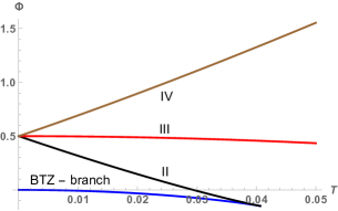
Figure 3: The grand potential for the four branches of black holes with spin-three chemical potential $\mu$. Here $\mu=1$, $T$ the temperature, and the grand potential is plotted as a function of the dimensionless parameter $\mu T$ .

It was found in paper1 that thermal boundary conditions for the ${\mathfrak{sl}}(3)$ Chern-Simons connections with spin three chemical potential admit four distinct branches, only one of which is smoothly connected to the BTZ black hole in the limit of vanishing chemical potential. The free energy of the BTZ branch can be expanded in powers of $\mu T$ and can be shown to agree precisely with results from large-$c$ limit of CFT with ${W}_{3}$ symmetry. As displayed in figure 3, the BTZ branch merges with Branch II and then ceases to exist beyond a critical value of $(\mu T)$. Of the two remaining branches, Branch III is thermodynamically favoured and its high $T$ limit expected to match the thermodynamics of a large-$c$ CFT with ${W}_{3}^{(2)}$ symmetry. Our original motivation was to understand from a CFT perspective, certain intriguing aspects of this (UV) theory.

3.1 $W^{(2)}_{3}$ algebra and semiclassical limit

In this section we discuss relevant features of the Polyakov-Bershadsky algebra and its semiclassical limit. The main purpose of this section is to point out that the semiclassical limit of this algebra, in the Ramond sector, has an immediate interpretation which nontrivially matches the dual AdS bulk black hole description in terms of the flat connections of ${\rm SL}(3,{\mathbb{R}})\times{\rm SL}(3,{\mathbb{R}})$ Chern-Simons theory.

The best understood series of $W$-algebra CFTs are these with conventional $W_{N}$-algebras which can be seen to arise via the GKO coset construction GKO , or alternatively using Drinfel’d-Sokolov (DS) reduction DS . Such reductions are assocated to ${\mathfrak{sl}}(2)$ embeddings in ${\mathfrak{sl}}(N)$ and conventional $W_{N}$-algebras are associated to the principal emebdding of ${\mathfrak{sl}}(2)$ in ${\mathfrak{sl}}(N)$. However, the DS construction can be generalized to other ${\mathfrak{sl}}(2)$ embeddings. For $N=3$, one such non-principal embedding yields the $W_{3}^{(2)}$-algebra. In a CFT with $W^{(2)}_{3}\times W^{(2)}_{3}$ symmetry, the algebra is realized via the OPE of the stress tensor $T(z)$, two spin-$\frac{3}{2}$ currents $G^{\pm}(z)$ and a $U(1)$ current $J(z)$:

$$T(z)T(0)\,=\,\frac{c}{2z^{4}}+\frac{2T(0)}{z^{2}}+\frac{\partial T(0)}{z}+\cdots\$$ (71)

$$T(z)J(0)\,=\,\frac{J(0)}{z^{2}}+\frac{\partial J(0)}{z}+\cdots\,,\qquad T(z)G^{\pm}(0)=\frac{3G^{\pm}(0)}{2z^{2}}+\frac{\partial G^{\pm}(0)}{z}+\cdots\,,$$

$$J(z)J(0)\,=\,\frac{\kappa}{z^{2}}+\cdots\ ,\qquad\qquad\qquad\,\,J(z)G^{\pm}(0)\,=\,\pm\frac{G^{\pm}(0)}{z}+\cdots\,,$$

$$G^{+}(z)G^{-}(0)\,=\,\frac{(k-1)(2k-3)}{\,z^{3}}\,-\,\frac{3(k-1)J(0)}{\,z^{2}}$$

$$\qquad\qquad\qquad\qquad\qquad\qquad+\,\frac{1}{z}\left((k-3){T(0)\,+\,3:J(0)^{2}:\,-\,\frac{3}{2}(k-3)\partial J(0)}\right)\,+\,\cdots\$$

where $k$ is related to the level of the ${\mathfrak{sl}}(3)$ affine algebra and the central charge $c$ is given by

$$c\,=\,\frac{(2k-3)(3k-1)}{k-3}\ ,\qquad\kappa\,=\,-\frac{2k-3}{3}\,.$$ (72)

In the context of AdS₃/CFT₂ duality for higher spin theory, $k$ is the level of the ${\rm SL}(3,{\mathbb{R}})\times{\rm SL}(3,{\mathbb{R}})$ Chern-Simons theory in the bulk dual. The semiclassical limit for the latter requires

$$c\to\infty,\qquad k\to\infty\,,\qquad c\,=\,6k\,.$$ (73)

In this limit however, the level of the $U(1)$ current algebra $\kappa\,\to\,-2k/3$ becomes negative and large and thus the corresponding CFT cannot be unitary.

Using the (Laurent) mode expansions for the currents,

$$J(z)\,=\,\sum_{n}z^{-n-1}J_{n}\,,\qquad G^{\pm}(z)\,=\,\sum_{n}z^{-n-\frac{3}{2}}G^{\pm}_{n}\,,\qquad T(z)\,=\,\sum_{n}z^{-n-2}L_{n}\,,$$ (74)

we can represent the algebra in terms of the commutation relations for the modes (160). Although the currents $G^{\pm}$ have half-integer spin, they are bosonic and the algebra is nonlinear. The half-integer spin fields allow for both integer (Ramond) and half-integer (Neveu-Schwarz) modings.

3.2 Ramond sector zero mode algebra and the semiclassical limit

Let us focus attention on the Ramond sector where $G_{n}^{\pm}$ are integer moded, and in particular, on the zero mode sector spanned by $\{L_{0},G_{0}^{\pm},J_{0}\}$. The algebra of the zero modes,

$$\left[L_{0},J_{0}\right]\,=\,\left[L_{0},G_{0}^{\pm}\right]\,=\,0\,,\qquad\left[J_{0},G_{0}^{\pm}\right]\,=\,\pm G_{0}^{\pm}\,,$$ (75)

$$\left[G_{0}^{+},G_{0}^{-}\right]\,=\,-\frac{(k-1)(2k-3)}{8}\,+(k-3)L_{0}\,+\,3J_{0}^{2}\,,$$

has two Casimirs which label a given representation: the first is $L_{0}\,=\,\Delta\mathds{1}$ which yields the conformal dimension, while the second Casimir is

$$\tfrac{1}{2}\{G_{0}^{+},G_{0}^{-}\}\,+\,J_{0}^{3}\,+\,\left((k-3)L_{0}\,+\,\tfrac{1}{2}-\tfrac{(k-1)(2k-3)}{8}\right)\,J_{0}\,=\,\Delta^{(3)}\mathds{1}\,,$$ (76)

where the first term on the left hand side is the anticommutator of the two zero modes. The representations of the zero mode algebra have a structure that is quite similar to that of $SU(2)$. Highest weight states $|\psi\rangle$ in the Ramond sector come in degenerate multiplets spanned by the states $\left(G_{0}^{+}\right)^{j}|\psi\rangle$obtained by the action of the raising operator. For an irreducible representation ${\cal R}$ of dimension $n$, the generators of the zero mode algebra can be represented as $n\times n$ matrices (see Arakawa:2010sc ):

$$J_{0}\,=\,y\,{\mathds{1}}_{n\times n}\,+\,{\rm diag}\left(\tfrac{n-1}{2},\,\tfrac{n-3}{2},\ldots,-\tfrac{n-1}{2}\right)\,,\qquad L_{0}\,=\,\Delta\,\mathds{1}_{n\times n}$$ (77)

$$\left(G_{0}^{+}\right)_{\ell,j}\,=\,\sqrt{j(n-j)\left(3y+\tfrac{n}{2}-j\right)}\,\delta_{j,\ell+1}\,,\qquad G_{0}^{-}\,=\,\left(G_{0}^{+}\right)^{\dagger}\,,\qquad\ell=1,2\ldots n-1\,.$$

The conformal dimension $\Delta$ and the second Casimir $\Delta^{(3)}$ can be epxressed in terms of the three quantum numbers $(k,n,y)$ as

$$\Delta\,=\,\frac{1}{8(k-3)}\left((2k-3)(k-1)+2-2n^{2}-24y^{2}\right)\,,\qquad\Delta^{(3)}\,=\,\frac{1}{2}y\left(n^{2}-4y^{2}\right)\,.$$ (78)

In the large-$k$ semiclassical limit, the central charge $c\to 6k$, and letting both $n$ and $y$ scale with $k$, we find

$$\left.\Delta\right|_{k\gg 1}\to\,\frac{c}{24}\,-\,\frac{3n^{2}}{2c}\,-\,\frac{18y^{2}}{c}\,.$$ (79)

Thus the conformal weights of the highest weight states are negative definite in this limit.

It is useful to rewrite the Casimirs in terms of the highest weight vectors ${\bf\Lambda}$ used to label the corresponding representations. In terms of these the conformal dimensions of the highest weight states (in the Ramond sector) is given by Arakawa:2010sc

$$\Delta\,=\,\frac{{\bf\Lambda}\cdot\left({\bf\Lambda}\,+\,2{\bm{\rho}}\right)}{2(3-k)}\,-\,\tilde{\bm{\nu}}\cdot{\bf\Lambda}\,+\,\frac{\kappa}{8}\,.$$ (80)

Here ${\bm{\rho}}$ is the Weyl vector, given by the sum of the fundamental weights $({\bm{w}_{1}},{\bm{w}_{2}})$ and $\tilde{\bm{\nu}}={\bm{w}_{2}}$ for for ${\mathfrak{sl}}(3)$. A convenient basis for the weight space of ${\mathfrak{sl}}(3)$ is provided by the three linearly dependent vectors $({\bm{e}_{1}},{\bm{e}_{2}},{\bm{e}_{3}})$ satisfying $\sum_{i}{\bm{e}_{i}}=0$ and

$$\langle{\bm{e}_{i}},{\bm{e}_{j}}\rangle\,=\,\delta_{ij}\,-\,\frac{1}{3}\,.$$ (81)

In terms of these, the fundamental weights of ${\mathfrak{sl}}(3)$ are ${\bm{w}}_{1}\,=\,{\bm{e}}_{1}$ and ${\bm{w}}_{2}\,=\,{\bm{e}}_{1}+{\bm{e}}_{2}$. The highest weight vector ${\bm{\Lambda}}$ can be expressed in this basis as

$${\bm{\Lambda}}\,=\,\left(-k+1+\frac{n}{2}+3y\right)\,{\bm{e}}_{1}\,+\,\left(-k+2-\frac{n}{2}+3y\right)\,{\bm{e}}_{2}\,.$$ (82)

From this, it is clear that the dimension of the representation is also determined compactly in terms of ${\bm{\Lambda}}$,

$$n\,=\,({\bm{e}}_{1}-{\bm{e}}_{2})\cdot{\bm{\Lambda}}\,+\,1\,.$$ (83)

In the semiclassical limit of large $k$, it is thus natural to take both the dimension of the representation $n$ and the parameter $y$ to scale with $n$, so that

$${\bm{\Lambda}}\xrightarrow{k\to\infty}k\,{\bm{\Lambda}}_{-}\,,\qquad{\bm{\Lambda}}_{-}\,\equiv\,\frac{n}{2k}({\bm{e}}_{1}-{\bm{e}}_{2})-\left(\tfrac{3y}{k}-1\right)\,{\bm{e}}_{3}\,.$$ (84)

The Weyl vector for ${\mathfrak{sl}}(3)$ is independent of $k$ and thus can be neglected in the formula for $\Delta$ in this limit. An immediate consequence of this is that both the Casimirs $\Delta$ and $\Delta^{(3)}$ depend only on the combination ${\bm{\omega}}\,=\,{\bm{\Lambda}}_{-}+\tilde{\bm{\nu}}$. Viewing ${\bm{\omega}}$ as a vector in ${\mathbb{R}}^{3}$ with components $(\omega_{1},\omega_{2},\omega_{3})$, we define the quantities

$$C_{s}({\bm{\omega}})\,=\,\frac{1}{s}\sum_{i=1}^{3}\omega_{i}^{s}\,.$$ (85)

Thus we may write the Casimir conditions for the ground states (in the semiclassical limit) as

$$\langle L_{0}\rangle-\,\frac{c}{24}\,\xrightarrow{k\to\infty}\,-k\,C_{2}({\bm{\omega}})\,,$$ (86)

$$\Delta^{(3)}\mathds{1}\xrightarrow{k\to\infty}\left\langle\tfrac{1}{2}\{G_{0}^{+},G_{0}^{-}\}\,+\,J_{0}^{3}\,+\,\frac{c}{6}\,J_{0}\left(L_{0}\,-\tfrac{c}{24}\right)\right\rangle\,=\,k^{3}\,C_{3}({\bm{\omega}})\,.$$

We note that in the semiclassical limit, the dimension of the representation becomes infinite as $n\sim{\cal O}(k)$, and the zero mode matrices $(J_{0},G_{0}^{\pm})$ effectively commute. In particular, the scaling of the off-diagional entries in eq.(77) implies that $G_{0}^{\pm}\sim{\cal O}(k^{3/2})$, while $L_{0}\sim{\cal O}(k)$ and $J_{0}\sim{\cal O}(k)$ in the large-$k$ limit, and the commutator $[G_{0}^{+},G_{0}^{-}]$ is thus subleading. Therefore, the limit of large $k$ is semiclassical in nature, wherein the correspondence principle applies and the zero mode operators can be replaced by $c$-numbers and the Casimir conditions viewed as algebraic equations.

We are interested in comparing the large-$k$ formulae with corresponding results for the spin-$\frac{3}{2}$ black hole obtained in paper1 using the Chern-Simons formulation. In order to make this comparison, we perform certain rescalings and define

$$\langle{G^{\pm}_{0}}\rangle\,=\,\pm i^{3/2}\pi\sqrt{\frac{k}{{2}}}{\cal G}^{\pm}\,,\qquad\langle J_{0}\rangle\,=\,iq,\qquad{\cal E}\,=\,\langle L_{0}\rangle\,-\,\frac{c}{24}\,.$$ (87)

The factors of $i$ appear when connecting the expectation values of the zero modes on the $z$-plane, to those on the cylinder using the map $z=e^{iw}$. The minus sign and the factor of $\sqrt{k}$ have also been introduced in order to match with the conventions for the expectation values of the $W_{3}^{(2)}$ currents on the cylinder in paper1 . The Casimir conditions are thus,

$$\boxed{{\cal E}\,=\,-k^{-1}\left(\frac{n^{2}}{4}\,+\,3y^{2}\right)\,,}$$ (88)

$$\boxed{\frac{\pi^{2}}{2}{\cal G}^{+}{\cal G}^{-}\,-\,k^{-1}q^{3}\,+\,q\,{\cal E}\,=\,-\frac{i}{2k}y(n^{2}-4y^{2})\,.}$$

We will demonstrate two important results below:

1. The left hand sides of the two Casimir equations are to be identified with the traces of the square and the cube of the ${\rm SL}(3,\mathbb{R})$ Chern-Simons connection which determines the higher spin dual gravity background.

2. The flatness requirement for the Chern-Simons connection corresponds to picking the saddle point of the path integral over the manifold (at large $k$) of zero mode ground states in the Ramond sector.

3.3 Chern-Simons bulk dual at large $c$

The holographic description of a $W_{3}^{(2)}$ CFT at large central charge is given by Chern Simons theory with ${\rm SL}(3,{\mathbb{R}})\times{\rm SL}(3,{\mathbb{R}})$ gauge group and gauge connections $A(w,\bar{w},\rho)$ and $\bar{A}(w,\bar{w},\rho)$. The $\rho$ coordinate has the intepretation of the radial direction in ${\rm AdS}_{3}$ spacetime and for translationally invariant states in the CFT, the dependence can be factored out, and the connections replaced by gauge equivalent constant matrices $(a,\bar{a})$:

$$A\,=\,b^{-1}a\,b+b^{-1}db,\qquad\bar{A}\,=\,b\,\bar{a}\,b^{-1}+b\,db^{-1}\,,\qquad b\,=\,e^{\rho\hat{L}_{0}}\,.$$ (89)

Here $\hat{L}_{0}$ is the dilatation generator associated to the ${\mathfrak{sl}}(2)$ algebra in the appropriate non-principal embedding in ${\mathfrak{sl}}(3,{\mathbb{R}})$. The constant connections $(a,\bar{a})$ each have two components:

$$a\,=\,a_{w}\,dw\,+\,a_{\bar{w}}\,d\bar{w}\,,\qquad\qquad\bar{a}\,=\,\bar{a}_{w}\,dw\,+\,\bar{a}_{\bar{w}}\,d\bar{w}\,,$$ (90)

where $a_{\bar{w}}$ and $\bar{a}_{w}$ are non-vanishing only when a chemical potential $\lambda$ for spin-$\tfrac{3}{2}$ charge is turned on. We define the matrices $\{\hat{L}_{0},\hat{L}_{\pm 1},J_{0},G^{\pm}_{1/2},G^{\pm}_{-1/2}\}$ in terms of ${\rm SL}(3,\mathbb{R})$ generators as in (161). For the moment we ignore the chemical potential and focus attention on the holomorphic component $a_{w}$ and its antiholomorphic counterpart in the barred sector $\bar{a}_{\bar{w}}$. Following the conventions in paper1 , the relevant gauge connection (in highest weight gauge Gutperle:2011kf ) is:

$$a_{w}\,=\,\left[\hat{L}_{1}+\frac{3q}{2k}J_{0}-\frac{w_{-2}}{k}\hat{L}_{-1}+\frac{\pi}{\sqrt{2}k}\left({\cal G}^{+}G^{+}_{-1/2}\,+\,{\cal G^{-}}G^{-}_{-1/2}\right)\right]$$ (91)

and similarly in the barred sector

$$\bar{a}_{\bar{w}}\,=\,-\,\left[\hat{L}_{-1}-\frac{3q}{2k}J_{0}\,-\,\frac{w_{-2}}{k}\hat{L}_{1}-\frac{\pi}{\sqrt{2}k}\left({\cal G}^{-}G^{-}_{1/2}\,-\,{\cal G}^{+}G^{+}_{1/2}\right)\right]\,.$$ (92)

In paper1 , by matching the Chern-Simons equations of motion to Ward identities of the $W_{3}^{(2)}$ algebra, it was shown that ${\cal G}^{\pm}$ and $q$ are the expectation values of the spin-$\frac{3}{2}$ currents and the $U(1)$ current respectively, while $w_{-2}$ is the expectation value of the ‘improved’ stress tensor,

$$w_{-2}\,=\left\langle-T(w)-\frac{3}{4k}J(w)^{2}\right\rangle\,=\,{\cal E}\,-\,\frac{3q^{2}}{4k}\,.$$ (93)

Both $a_{w}$ and ${\bar{a}}_{\bar{w}}$ are traceless. However, the higher traces are non-vanishing:

$$\boxed{\tfrac{1}{2}{\rm Tr}\,a_{w}^{2}\,=\,\tfrac{1}{k}\left(w_{-2}\,+\,\tfrac{3q^{2}}{4k}\right)}\,,\qquad\boxed{\tfrac{1}{3}{\rm Tr}\,a_{w}^{3}\,=\,\tfrac{1}{k^{2}}\left(\tfrac{\pi^{2}}{2}\,{\cal G}^{+}{\cal G}^{-}\,-\,\tfrac{q^{3}}{4k}\,+\,{w_{-2}}\,q\right)}\,.$$ (94)

It is clear that these have the same form as the quadratic and cubic Casimirs (88) of the zero mode algebra of $W_{3}^{(2)}$ we encountered above, upon making the identification,

$${\cal E}\,=\,\left(w_{-2}\,+\,\tfrac{3q^{2}}{4k}\right)\,,$$ (95)

exactly as indicated by eq.(93).

The Chern-Simons bulk description of the CFT state requires two further inputs. The first is the flatness of the connection, and the second is the smoothness requirement which constrains the holonomy of the gauge fields around the compact spatial direction or the compact (Euclidean) temporal circle in the thermal state. When the holonomy is nontrivial (or non-smooth) we interpret the corresponding state as a conical deficit/excess. The flatness condition is simple in the absence of a chemical potential (i.e. when $a_{\bar{w}}=\bar{a}_{w}=0$). At zero temperature, the holonomy of the gauge field around the spatial circle must be trivial, corresponding to the higher spin version of global ${\rm AdS}_{3}$,

$${\rm Hol}_{\phi}(A)\,\equiv\,{\cal P}\exp\left(\oint A_{\phi}\right)\,=\,\mathds{1}\,,$$ (96)

where

$$A_{\phi}\,=\,A_{w}\,-\,A_{\bar{w}}\,,\qquad A_{t}\,=\,i\left(A_{w}\,+\,A_{\bar{w}}\right)\,.$$ (97)

For the zero temperature ground state, this fixes the eigenvalues of $a_{\phi}$:

$${\rm spec}(a_{\phi})\,=\,(i,0,-i)\,.$$ (98)

Since $a_{\bar{w}}=0$ in the absence of chemical potential deformatons, this implies that the ground state corresponds to an operator $\Phi$ with non-trivial (negative) conformal dimension

$${\cal E}\,=\,-\frac{c}{6}\,\implies\,\Delta_{\Phi}\,=\,\frac{c}{24}\,-\,\frac{c}{6}\,=\,-\frac{c}{8}\,.$$ (99)

Note that there are two zero mode states labelled by the quantum numbers $(y,n)$ with this energy and holonomy in the semiclassical limit, namely $(y,n)\,=\,(0,2k)$ and $(y,n)\,=\,(k/2,\,k)$. Both allowed solutions are highly degenerate and in the large $k$ limit, the family of ground states is characterized by the algebraic variety (88).

Next we turn to the CFT in the thermal state. At high temperatures in the semiclassical limit, modular invariance tells us that the spatial circle at zero temperature is swapped for the Euclidean thermal circle with circumference $\beta$. However, since the zero temperature ground state(s) have nontrivial conformal dimension $\Delta_{\Phi}\,=\,-\frac{c}{8}$ (99), we expect that the thermal cylinder is accompanied by insertions of a primary operator $\Phi$ at spatial infinity. Furthermore the manifold of ground states at zero temperature (given by the algebraic variety at large-$c$ spanned by the zero mode sector) now has a thermal counterpart given by the smoothness conditions for the holonomy around the thermal circle:

$${\rm Hol}_{t}(A)\,=\,{\cal P}\exp\left(\oint A_{t}\right)\,=\,\mathds{1}\,\implies\,{\rm spec}(a_{t})\,=\,\left(2\pi i\beta^{-1},\,0,\,-2\pi i\beta^{-1}\right)\,.$$ (100)

Therefore the constraints on the quadratic and cubic Casimirs are,

$${\cal E}\,=\,k\frac{4\pi^{2}}{\beta^{2}}\,\qquad\qquad\frac{\pi^{2}}{2}{\cal G}^{+}{\cal G}^{-}\,-\,k^{-1}q^{3}\,+\,{\cal E}q\,=\,0\,.$$ (101)

With $k\,=\,c/6$, this is the expected high temperature behaviour for the CFT with rescaled temperature $\beta_{\Phi}\,=\,\beta/2$ as in (20).

3.4 Grand canonical saddle point and flat C-S connections

We now introduce a bias in the system via a small chemical potential for the spin-$\tfrac{3}{2}$ currents. At the level of the CFT action this is a holomorphic (plus antiholomorphic) deformation

$$\delta I_{\rm CFT}\,=\,-\lambda\int_{S^{1}\times{\mathbb{R}}_{t}}d^{2}w\,\left(g_{+}\,{G^{+}}(w)\,+\,g_{-}\,{G^{-}}(w)\right)\,+\,{\rm h.c.}$$ (102)

where $\lambda$ is a dimension-$\frac{1}{2}$ chemical potential and $g_{\pm}$ are dimensionless parameters. For simplicity we set $g_{+}=g_{-}$. In the dual bulk Chern-Simons theory, the deformation modifies the gauge connections so that $a_{\bar{w}}\neq 0$ and ${\bar{a}}_{w}\neq 0$ as in paper1 ,

$$a_{\bar{w}}\,=\,\,\lambda\left[\sqrt{2}\left(G^{-}_{1/2}-G^{+}_{1/2}\right)+\frac{3q}{\sqrt{2}k}\left(G^{+}_{-1/2}+G^{-}_{-1/2}\right)+\frac{\pi{\cal G}}{k}\hat{L}_{-1}\right]$$ (103)

$$\bar{a}_{w}\,=\,\lambda\left[\sqrt{2}\left(G^{+}_{-1/2}+G^{-}_{-1/2}\right)+\frac{3q}{\sqrt{2}k}\left(G^{-}_{1/2}-G^{+}_{1/2}\right)-\frac{\pi{\cal G}}{k}\hat{L}_{1}\right]\,,$$

and the flatness condition $[a_{w},a_{\bar{w}}]\,=\,[\bar{a}_{w},{\bar{a}}_{\bar{w}}]\,=\,0$, then constrains the expectation values of the improved stress tensor (93) and the spin-$\tfrac{3}{2}$ charges,

$$w_{-2}\,=\,\frac{9q^{2}}{4k}\,,\qquad\qquad{\cal G}\,=\,\langle g_{+}G^{+}\rangle\,=\,\langle g_{-}G^{-}\rangle\,.$$ (104)

Interestingly, both conditions can be understood as a consequence of a large-$k$ saddle point of the path integral over the zero mode ground states in the Ramond sector. In particular, let us consider schematically the path integral (at large $k$) over the zero modes. The small $\lambda$ limit is best understood as a high temperature limit where $\lambda\sqrt{\beta}\ll 1$ and we make use of the high temperature versions of the Casimir conditions (or holonomies)

$${\cal Z}\,\sim\,\int d{\cal E}\,dq\,d{\cal G}^{+}\,d{\cal G}^{-}\,\times$$ (105)

$$\delta\left({\cal E}\,-\,\tfrac{4\pi^{2}}{\beta^{2}}k\right)\,\delta\left(\frac{\pi^{2}}{2}{\cal G}^{+}{\cal G}^{-}-k^{-1}q^{3}+q{\cal E}\,\right)\,e^{-\beta\ell\lambda\left({\cal G}^{+}+{\cal G}^{-}\right)}\,\ldots$$

The ellipsis represent any other factors in the partition sum including putative higher order terms in $\lambda$ and we have introduced an explicit dimensionful factor $\ell$ representing the size of the spatial circle. Also omitted are finite $\lambda$ corrections to the holonomy conditions which can be found in paper1 . Implementing the delta-functions constraints via Lagrange multipliers and locating the saddle point with respect to $q$, ${\cal G^{\pm}}$, ${\cal E}$ and the Lagrange multipliers, which dominates the integral at large $k$ and high temperatures, we find in the $\lambda\to 0$ limit:

$${\cal E}\,=\,\frac{3}{k}q^{2}\,,\qquad{\cal G}^{+}\,=\,{\cal G}^{-}\,,$$ (106)

which, after using (93), reduces precisely to the conditions (104) resulting from imposing the flatness of the Chern-Simons connection at finite (small) chemical potential $\lambda$.

To summarize, we have provided evidence above that the classical, large-$c$ holographic dual of a CFT with ${W}_{3}^{(2)}$ symmetry has a large degeneracy of states which appear as a continuum in the large-$c$ limit, with a large negative conformal dimension. The large-$c$ manifold of ground states is given by the algebraic variety (88).

3.5 Ward identities for finite $\lambda$

In this subsection, for the sake of completeness, we recall the analysis presented in paper1 where it was shown that Ward identities of the large-$c$ ${W}^{(2)}_{3}$ CFT with spin-$\tfrac{3}{2}$ chemical potential $\lambda$, are reproduced by the bulk Chern-Simons field equations,

$$da+a\wedge a=0,\qquad d\bar{a}+\bar{a}\wedge\bar{a}=0.$$ (107)

We impose the flatness conditions on the connections $a=a_{w}\,dw\,+\,a_{\bar{w}}\,d\bar{w}$ and $\bar{a}=\bar{a}_{w}\,dw\,+\,\bar{a}_{\bar{w}}\,d\bar{w}$ treating their parameters $(q,w_{-2},{\cal G})$ as functions of $(w,\bar{w})$ with $w\,=\,\phi\,+\,it$. This yields the set of first order equations:

$$\partial_{\bar{w}}\left(w_{-2}\,+\,\frac{3}{4k}\,q^{2}\right)\,=\,-\pi\lambda\,\partial_{z}{\cal G},\qquad\qquad\partial_{\bar{z}}q=-4k\lambda\,w_{-1}\,,$$ (108)

$$\partial_{\bar{w}}w_{-1}\,=\,\tfrac{\lambda}{k}\left(-w_{-2}+\frac{9}{4k}q^{2}\right),\qquad\qquad\partial_{\bar{w}}{\cal G}\,=\,\tfrac{3}{\pi}\,\lambda\,\partial_{w}q\,.$$

These conditions are equivalent to the Ward identities of the CFT with ${W}^{(2)}_{3}$ symmetry, deformed by a spin-$3/2$ current,

$$\delta I_{\rm CFT}\,=\,-\int_{S^{1}\times{\mathbb{R}}_{t}}d^{2}w\lambda(\bar{w})\left(g_{+}G^{+}(w)+g_{-}G^{-}(w)\right)\,.$$ (109)

The Ward identities of this deformed theory are obtained by computing the expectation values of the left hand sides of (108) pertubatively in $\lambda$, using the identity $\partial_{\bar{w}}\left(\frac{1}{w}\right)\,=\,2\pi\delta^{2}(w,\bar{w})$ and the OPEs of the currents (71),

$$\tfrac{1}{2\pi}\partial_{\bar{w}}\langle T(w)\rangle_{\lambda}\,=\,\tfrac{1}{2}\lambda\,\partial_{w}\langle g_{+}G^{+}(w)\,+\,g_{-}G^{-}(w)\rangle$$ (110)

$$\tfrac{1}{2\pi}\partial_{\bar{w}}\langle J(w)\rangle_{\lambda}\,=\,-\lambda\,\langle g_{+}G^{+}(w)\,-\,g_{-}G^{-}(w)\rangle$$

$$\tfrac{1}{2\pi}\partial_{\bar{w}}\langle g_{+}G^{+}(w)\,-\,g_{-}G^{-}(w)\rangle_{\lambda}\,=\,2g_{+}g_{-}\lambda\,\langle T(w)\,+\,\tfrac{18}{c}J(w)^{2}\rangle$$

$$\tfrac{1}{2\pi}\partial_{\bar{w}}\langle g_{+}G^{+}(w)+g_{-}G^{-}(w)\rangle_{\lambda}\,=\,3g_{+}g_{-}\lambda\,\partial_{w}\langle J(w)\rangle.$$

These Ward identities show that the $W_{3}^{(2)}$ currents are not actually holomorphic after the chiral deformation (109) is introduced. Comparing these with the bulk field equations (108), the CFT expectation values of the currents can be identified in terms of bulk quantities,

$$w_{-1}\,=\,\frac{\pi}{2k}\langle g_{+}G^{+}(w)\,-\,g_{-}G^{-}(w)\rangle_{\lambda},\qquad{\cal G}\,=\,\langle g_{+}G^{+}(w)+g_{-}G^{-}(w)\rangle_{\lambda}$$ (111)

$$w_{-2}=\langle-T(w)\,-\,\frac{3}{4k}J(w)^{2}\rangle_{\lambda},\qquad\qquad q\,=\,\langle J(w)\rangle_{\lambda},\qquad g_{+}g_{-}=\frac{1}{2\pi^{2}}.$$

In the following sections, we will consider situations both with $\lambda$ zero and non-zero from within the holographic large-$c$ description, and match with our CFT interpretation.

4 Zero charge $W^{(2)}_{3}$ black hole

4.1 Thermodynamics

We now turn our attention to the thermodynamical properties of the holographic large-$c$ theory in the canonical ensemble ($\lambda=0$). We have seen that the high temperature energy of this thermal state is given by (summing over both holomorphic and antiholomorphic sectors)

$$-\langle T\rangle\,-\,\langle\bar{T}\rangle\,=\,2{\cal E}\,=\,c\,\frac{4\pi^{2}}{3\beta^{2}}\,,$$ (112)

which then corresponds to the thermal entropy

$$S\,=\,c\,\frac{8\pi^{2}}{3\beta}\,.$$ (113)

Both quantities above are a factor of 4 times the expected result for a BTZ black hole (or high temperature CFT) at temperature $\beta^{-1}$. The constant Chern-Simons connections for the zero charge black hole in the non-principal embedding are:

$$a=\left(\hat{L}_{1}-\frac{w_{-2}}{k}\hat{L}_{-1}\right)dw,\qquad\bar{a}=-\left(\hat{L}_{-1}-\frac{w_{-2}}{k}\hat{L}_{1}\right)d\bar{w}\,.$$ (114)

These have the same form as those for the BTZ black hole, the crucial difference being the non-principal embedding of ${\mathfrak{sl}}(2)$ generators $\{\hat{L}_{\pm 1},\hat{L}_{0}\}$ in the ${\mathfrak{sl}}(3)$ algebra (see appendix 161). Our interpretation of this difference is that it is a consequence of the large (negative) conformal dimension of the zero temperature ground state. The high temperature expectation value of the stress tensor in this situation follows from the CFT result (18),

$$\langle T\rangle_{\beta,{\Phi}}\,=\,\left(\frac{2\pi}{\beta}\right)^{2}\Delta_{\Phi}\,-\,\frac{c\pi^{2}}{6\beta^{2}}\,=\,-c\,\frac{2\pi^{2}}{3\beta^{2}}\,,$$ (115)

where $\Delta_{\Phi}\,=\,-\frac{c}{8}$ is the conformal dimensionof the zero temperature ground state (99). The insertion of this primary on the high temperature thermal cylinder leads to the standard high temperature thermodynamics, but at a larger rescaled temperature $\beta_{\Phi}\,=\,\beta/2$.

4.2 Entanglement entropy

From holography:

The prescription for computing the entanglement entropy in the Chern-Simons formulation of gravity with higher spin fields involves the calculation of a bulk (AdS₃) Wilson line in a specific representation ${\cal R}$, anchored at the endpoints $P$ and $Q$ of the entangling interval on the boundary CFT deBoer:2013vca ; Ammon:2013hba ,

$$S_{\rm EE}(P,Q)\,=\,\frac{k}{\sigma_{1/2}}\,\ln\left[\lim_{\rho_{P},\rho_{Q}\to\infty}W_{\cal R}(P,Q)\right]\,,$$ (117)

$$W_{\cal R}(P,Q)\,=\,{\rm Tr}_{\cal R}\left[{\cal P}\,\exp\left(\int_{P}^{Q}\bar{A}\right)\exp\left(\int_{Q}^{P}A\right)\right]\,.$$

The proposal of deBoer:2013vca included an overall normalization constant $\sigma_{1/2}=2$ when the embedding yields half-integer spin currents, otherwise $\sigma_{1/2}=1$. The constant was introduced in order that the entanglement entropy agree with the thermal entropy for large intervals when the former becomes extensive. However, in the present context we will see below that this normalization is necessary for agreement with the short interval limit which is determined by the universal OPE for the twist operators (59).

Although this will not be important for us in this paper, the prescription for the Wilson line which matches the CFT evaluation of entanglement entropies Datta:2014ska ; Datta:2014uxa is the so-called “holomorphic” prescription deBoer:2013vca . The other “canonical” prescription reduces to the holomorphic one when $A_{\bar{w}}\,=\,\bar{A}_{w}\,=\,0$ which is the case when the chemical potential $\lambda$ is vanishing. In the ${\rm SL}(3,{\mathbb{R}})\times{\rm SL}(3,{\mathbb{R}})$ Chern-Simons theory the entanglement entropy for both the principal and non-principal embeddings is given by the Wilson line in the adjoint representation deBoer:2013vca ,

$${\rm dim}[{\cal R}]\,=\,8\,.$$ (118)

The Wilson line in the adjoint representation is obtained by the product of the Wilson lines in the fundamental and conjugate representations,

$$W_{\rm fund}\,=\,\lim_{\rho_{P},\rho_{Q}\to\infty}\text{Tr}\left[e^{\rho_{Q}\hat{L}_{0}}\,{\rm exp}\left(-\Delta\bar{w}\,\bar{a}\right)e^{-2\rho_{P}\hat{L}_{0}}\,{\rm exp}\left(\Delta w\,a\right)e^{\rho_{Q}\hat{L}_{0}}\right]\,,$$ (119)

$$W_{\rm Ad}\,=\,W_{\rm fund}\,W_{\overline{\rm fund}}\,.$$

The anti-fundamental Wilson line is identical to the fundamental Wilson line but with signs reversed in front of $\Delta w$ and $\Delta\bar{w}$. For the single interval entanglement entropy, $\Delta w=\Delta\bar{w}=L$, the size of the interval. In the limit of large $\rho_{P,Q}$ wherein the endpoints of the Wilson line are anchored to the boundary of AdS₃, we obtain,

$$W_{\rm Ad}\,=\,e^{2(\rho_{P}+\rho_{Q})}\,\frac{k^{2}}{w_{-2}^{2}}\sinh^{4}\left(\sqrt{\frac{w_{-2}}{k}}L\right)\,.$$ (120)

When the $U(1)$ charge is vanishing, the parameter $w_{-2}$ is identified with the energy of one chiral sector as in (93), and its value determined by the holonomy condition (101) at high temperature. After subtracting out the additive divergent piece proportional to the UV cutoff, the EE for a single interval of length $L$ is,

$$S_{\rm EE}\,=\,\frac{c}{3}\ln\left[\frac{\beta}{2\pi}\sinh\left(\frac{2\pi L}{\beta}\right)\right]\,.\qquad$$ (121)

The standard formula for the high temperature EE for a CFT is $S_{\rm EE}\,=\,\frac{c}{3}\ln\left(\sinh\frac{\pi L}{\beta}\right)$. The result for the $W_{3}^{(2)}$ CFT shows a subtle difference. The argument of the hyperbolic sine function is twice the usual result. We now interpret this as a consequence of the nontrivial ground state with $\Delta_{\Phi}\,=\,-\frac{c}{8}$ which manifests itself as a conical deficit or rescaled temperature $\beta_{\Phi}=\beta/2$ at high temperatures. It is clear that the EE for a general conical deficit (58), does not yield the thermal entropy (23) in the excited state in the limit of large interval size. However, the limit of small interval size precisely matches the OPE of twist operators (59).

Entanglement entropy from CFT:

We can evaluate the Rényi entropy in the CFT with ${\cal W}^{(2)}_{3}$ symmetry where the spin-$3/2$ and $U(1)$ charges are turned off. This is a non-standard situation because the ground state of the theory has a large negative conformal dimension. The conformal dimension of the twist fields cannot immediately be inferred by computing the stress tensor one-point function using the uniformisation map from a multi-sheeted Riemann surface implementing the replica trick. Each sheet is now accompanied by a pair of insertions of the primary field with conformal dimension $\Delta_{\Phi}$ corresponding to the nontrivial ground state. Instead we may view the Rényi entropy as a four-point correlator involving the two light branch point twist fields and two heavy primaries with $\Delta_{\Phi}\,=\,-\frac{c}{8}$. Assuming only the vacuum block contribution to the HHLL correlator, the Rényi entropy in the large-$c$ limit can be obtained as in section 2.2 and in the $n\to 1$ limit,

$$S_{\rm EE}\,=\,\frac{c}{3}\ln\left[\frac{\beta}{\pi\alpha_{\Phi}}\sinh\left(\alpha_{\Phi}\frac{\pi L}{\beta}\right)\right]\,,\qquad\alpha_{\Phi}\,=\,\sqrt{1-24\frac{\Delta_{\Phi}}{c}}\,.$$ (122)

Given $\Delta_{\Phi}=-\frac{c}{8}$, we recover the holographic EE (121).

5 $W^{(2)}_{3}$ black hole with spin-$3/2$ and $U(1)$ charges

The holonomy conditions (101) at high temperature show that the thermal states at fixed energy are highly degenerate, characterized by condensates or expectation values for the spin-$\tfrac{3}{2}$ and $U(1)$ charges. In general, we expect that the entanglement entropy will depend on the choice of state. However, the quantum theory sums over all these states and the resulting saddle point at large $k$ determines the thermodynamics. It is nevertheless interesting and instructive to consider any given solution to the holonomy conditions and compute the holographic EE for that configuration.

5.1 Holographic entanglement entropy for $W_{3}^{(2)}$ CFT

The general result for the $W_{3}^{(2)}$ Wilson line in the fundamental representation in terms of the eigenvalues of $a_{w}$ is,

$${W}_{\rm fund}\,= \frac{e^{\rho_{P}+\rho_{Q}}}{(\lambda_{1}\lambda_{2}\lambda_{3})^{2}}\times$$

$$\left[\lambda_{1}\left(\frac{q}{k}+\nu_{3}\right)e^{\nu_{3}\Delta w}+\lambda_{2}\left(\frac{q}{k}+\nu_{1}\right)e^{\nu_{1}\Delta w}+\lambda_{3}\left(\frac{q}{k}+\nu_{2}\right)e^{\nu_{2}\Delta w}\right]\times$$

$$\left[\lambda_{1}\left(\frac{q}{k}+\nu_{3}\right)e^{-\nu_{3}\Delta\bar{w}}+\lambda_{2}\left(\frac{q}{k}+\nu_{1}\right)e^{-\nu_{1}\Delta\bar{w}}+\lambda_{3}\left(\frac{q}{k}+\nu_{2}\right)e^{-\nu_{2}\Delta\bar{w}}\right]$$

where $\nu_{1,2,3}$ are eigenvalues of the matrix $a_{w}$ and the charges in the barred (91) and unbarred (92) sectors are identical. For the single interval entropy, $\Delta w=\Delta\bar{w}=L$ and we have defined

$$\lambda_{1}=\nu_{1}-\nu_{2},\qquad\lambda_{2}=\nu_{2}-\nu_{3},\qquad\lambda_{3}=\nu_{3}-\nu_{1}.$$ (124)

Since the barred and unbarred sectors are identical, the Wilson line in the antifundamental representation yields the same expression and $W_{\rm Ad}\,=\,\left(W_{\rm fund}\right)^{2}$. The expression above was obtained without imposing the holonomy conditions and applies for any values of $q,\,w_{-2}$ and ${\cal G}$. The $\{\nu_{i}\}$ are the roots of the cubic,

$$\nu^{3}\,-\,\frac{1}{k}\nu\left(w_{-2}\,+\,\frac{3q^{2}}{4k}\right)\,-\,\frac{1}{k^{2}}\left({\cal G}^{+}{\cal G}^{-}\frac{\pi^{2}}{2}\,-\,\frac{q^{3}}{4k}\,+\,qw_{-2}\right)\,=\,0\,.$$ (125)

The holonomy conditions (101) set the $\nu$-independent term in the cubic to zero and fix the coefficient of the term linear in $\nu$, so that the three eigenvalues are simply,

$$\left(\nu_{1},\nu_{2},\nu_{3}\right)=\left(-\tfrac{2\pi}{\beta},0,\tfrac{2\pi}{\beta}\right)\,,$$ (126)

for all values of $q,\,w_{-2}$ and ${\cal G}$ which satisfy the holonomy conditions. The holographic entanglement entropy is then expressible in a compact form for generic $q$:

$$S_{\rm EE}\,=\,\frac{c}{6}\ln\left[\frac{\beta^{4}}{(2\pi)^{4}}\sinh^{4}\left(\frac{2\pi L}{\beta}\right)\left(1-\frac{\beta^{2}}{4\pi^{2}}\frac{q^{2}}{k^{2}}{\rm tanh}^{2}\left(\frac{\pi L}{\beta}\right)\right)^{2}\right]\,.$$ (127)

We list the salient features of this result:

• When $q=0$, it reduces to eq.(121) as expected. The zero temperature version of this, for the CFT on the unit circle is obtained by the replacement $\beta\to-2\pi i$.

• The expression implies an upper bound on the $U(1)$ charge $q$ in terms of the temperature. Since $\tanh^{2}\tfrac{\pi L}{\beta}$ is monotonic in $L$, approaching unity as $L\to\infty$, if $|q|$ is too large the argument of the logarithm will have a zero at some finite value of $L$ and the EE will diverge at that point. In order to avoid this unphysical situation the $U(1)$ charge must be bounded:

  $$|q|\leq\frac{2\pi}{\beta}k\,.$$ (128)

  Interestingly, this bound is automatically implied by the dimension of the representation of the zero mode algebra in the semiclassical limit. Taking $y=0$ in eq.(77) the magnitude of the largest eigenvalue of $J_{0}$ is $n/2$ (taking $n$ large). From (87) and the Casimir condition (88) it immediately follows that

  $$q_{\rm max}^{2}\,=\,k{\cal E}\,=\,\left(\frac{2\pi k}{\beta}\right)^{2}\,.$$ (129)

• For generic values of $q$ below this bound, for large enough $L$, the EE is extensive but is lower than the thermal entropy (113) by a factor of two. This is a special case of what we have already noted for the EE of a conical deficit state (in the large-$c$ theory) (58).

• When the bound is saturated i.e. $|q|=2\pi k/\beta$, the expression for EE simplifies and surprisingly reduces to the standard CFT formula at finite temperature :

  $$S_{\rm EE}\,\big{|}_{|q|=\frac{2\pi k}{\beta}}\,=\,\frac{c}{3}\,\ln\left[\frac{\beta}{\pi}\,\sinh\left(\frac{\pi L}{\beta}\right)\right]\,.$$ (130)

  Importantly, the thermal entropy for the canonical ensemble is still given by (113) and does not agree with the EE of this particular configuration in the large $L$ limit.

• The smoothness/holonomy conditions (101) on the Chern-Simons connections relate the spin-$\tfrac{3}{2}$ charge to the $U(1)$ charge at a given temperature according to

  $$\frac{\pi^{2}}{2}{\cal G}^{+}{\cal G}^{-}\,=\,\frac{q}{k}\left(q^{2}\,-\,\frac{4\pi^{2}}{\beta^{2}}k^{2}\right)\,.$$ (131)

  

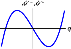
  Figure 4: The product ${\cal G}^{+}{\cal G}^{-}$ of the spin-$\tfrac{3}{2}$ charges versus the $U(1)$ charge $q$ for holographic backgrounds satisfying the holonomy conditions. ${\cal G}^{+}{\cal G}^{-}$ has extrema when $q^{2}=\tfrac{4}{3}\pi^{2}k^{2}\beta^{-2}$.

  Therefore the (product of) the spin-$\tfrac{3}{2}$ charges increases from zero at $q=0$, reaches a maximum at $q^{2}=4\pi^{2}k^{2}/3\beta^{2}$ and subsequently decreases to zero at $|q|=2\pi k/\beta$ (see figure 4).

• It is interesting to note what happens when an arbitrarily small spin-$\tfrac{3}{2}$ chemical potential $\lambda$ is introduced. The holonomy constraints (101) are then augmented with the Chern-Simons flatness (or large-$k$ saddle point) conditions (104) and this fixes the value of the $U(1)$ charge precisely at $q^{2}=\tfrac{4}{3}\pi^{2}k^{2}\beta^{-2}$, one of the two extrema of figure 4.

• The expansion of the holographic EE in the limit of small interval lengths has a nice interpretation:

  $$S_{\rm EE}\big{|}_{\frac{L}{\beta}\ll 1}\,=\,\frac{c}{3}\,\ln L\,+\,\frac{1}{3}\left(\frac{4\pi^{2}}{\beta^{2}}k\,-\,\frac{3q^{2}}{4k}\right)L^{2}\,+\ldots$$ (132)

  We immediately recognize the $O(L^{2})$ term as the expectation value of a particular combination of the stress tensor and the $U(1)$ current in the thermal state (with insertions of the operator $\Phi$ at spatial infinity),

  $$S_{\rm EE}\big{|}_{\frac{L}{\beta}\ll 1}\,=\,\frac{c}{3}\left(\ln\,L\,-\,\frac{L^{2}}{c}\left\langle T(w)\,+\,\frac{3}{4k}J(w)^{2}\right\rangle_{\Phi}\,+\ldots\right)\,.$$ (133)

  This has a natural interpretation in the CFT language as we now discuss.

5.2 Entanglement entropy from CFT at small $L$

Let us revisit the four-point correlator on the thermal cylinder which computes Rényi/entanglement entropy in CFT,

$${\cal C}_{4}\,=\,\frac{\langle\Phi(\infty)\,{\bar{\sigma}_{n}}(L){\sigma_{n}}(0)\,\Phi(-\infty)\rangle}{\langle\Phi(\infty)\,\Phi(-\infty)\rangle}\,.$$ (134)

The presence of the $U(1)$ current in the $W_{3}^{(2)}$ algebra permits the appearance of an additional quasi-primary $J^{2}$ of dimension two in the twist-antitwist OPE. This means that on general grounds the OPE of the twist fields must be of the form,

$${\bar{\sigma}_{n}}(L){\sigma_{n}}(0)\sim\frac{1}{L^{4h_{\sigma}}}\left(1+\frac{2h_{\sigma}}{c}L^{2}\left(T(0)\,+\,a\,J^{2}(0)\,+{\bar{T}}(0)\,+\,a\,{\bar{J}}^{2}(0)\right)\ldots\right)\,,$$ (135)

where $a$ is a dimensionless constant. There is a natural choice of $a$ from the viewpoint of the bulk Chern-Simons theory wherein the generators of the asymptotic symmetries of the metric commute with the generators of the $U(1)$ transformations. This corresponds to the choice of an effective stress tensor $T_{\rm eff}$ which has a trivial OPE with $J(z)$,

$$T_{\rm eff}(w)\,=\,T(w)\,+\,a\,J(w)^{2}\,,\qquad\qquad T_{\rm eff}(w)J(0)\,\sim\,{\rm regular}\,.$$ (136)

From the algebra (71), we can use the relevant large $k$ OPEs

$$T(w)J(0)\,\sim\,\frac{J(0)}{w^{2}}\,+\,\frac{\partial J(0)}{w}\,+\,\ldots\,,\qquad J(w)J(0)\,\sim\,-\frac{2k}{3w^{2}}\,+\ldots\,,$$ (137)

to immediately deduce that $a=3/(4k)$ and

$$T_{\rm eff}\,=\,T\,+\frac{3}{4k}J^{2}\,.$$ (138)

Inserting the OPE with the effective stress tensor modified by the Sugawara term into the four-point correlator for the Rényi entropy, we recover the short distance expansion (133) of the holographic EE at large-$c$ in the limit $n\to 1$.

6 OTO correlator and Lyapunov exponent

We are now in position to examine time dependent questions in this large-$c$ theory using the holographic prescription for higher spin entanglement entropy in the finite temperature CFT undergoing a local quench. The local quench is created by the insertion of a pair of primary operators at the origin at an instant of time. This leads to a time dependent change in the entanglement entropy of a spatial interval when the resulting excitations enter the interval. The holographic dual of this local quench is the backreacted solution for a black hole (thermal state) with an infalling massive particle, which starts its motion near the boundary and falls towards the black hole horizon. The mass $m$ of the infalling particle is proportional to the conformal dimension of the operator injecting the quench in the CFT.

In ordinary gravity the backreacted geometry associated to the infalling particle is obtained by a coordinate transformation and boost on a conical deficit state (see appendix C for these transformations) Caputa:2014eta . This is a so-called shockwave geometry. In higher spin gravity, the notions of metric and spacetime geometry are gauge dependent. Furthermore, the Wilson line prescription for the entanglement entropy is only sensitive to the location of the endpoints. For this reason, we only need to know the transformation of the endpoints of the Wilson line in a conical deficit background. For a detailed clarification of this point we refer the reader to David:2017eno . Here we present the method and the results.

6.1 Conical deficit

In Lorentzian signature, the endpoints of the entangling interval are given by light-cone coordinates $(w_{2},\bar{w}_{2})$ and $(w_{3},\bar{w}_{3})$ in eq.(2.3), while the locations of the operator insertions giving rise to the local quench are at $(w_{1},\bar{w}_{1})$ and $(w_{4},\bar{w}_{4})$. The operator insertions in imaginary time ($w_{1}=-i\epsilon$ and $w_{4}=i\epsilon$) have the effect of spreading out the pulse generated by the quench. The first step is to write down the Wilson line in a conical deficit state:

$$a\,=\,a_{-}\,d\xi^{-}\,,\qquad\qquad\bar{a}\,=\,\bar{a}_{+}\,d\xi^{+}\,.$$ (139)

where $a_{\mp}$ have exactly the same form as $a_{w}$ and $\bar{a}_{\bar{w}}$ respectively, in eqs.(91) and (92). For simplicity we take

$${\cal G}^{+}\,=\,{\cal G}^{-}\,=\,{\cal G}_{\cal O}\,\,,\qquad q\,=\,q_{\cal O}\,,$$ (140)

as the spin-$\tfrac{3}{2}$ and $U(1)$ charges of the state. The key point is that for a conical deficit state we do not impose smoothness conditions on the holonomy. Consequently, the holonomies are nontrivial and encoded in the traces. The energy of the conical deficit with respect to the non-trivial ground state of the CFT is proportional to $\delta_{\cal O}$ and is given by ${\rm Tr}\,a_{-}^{2}$ ,

$$\left(w_{-2}+\frac{3q^{2}}{4k}\right)\,=\,-\frac{c}{6}\left(1-\frac{\delta_{\cal O}}{c}\right)\,.$$ (141)

When $\delta_{\cal O}=0$ we recover the nontrivial ground state $|\Phi\rangle$ of the $W_{3}^{(2)}$ theory with $\Delta_{\Phi}=-\frac{c}{8}$. In order to compute the EE using the Wilson line prescription we need the eigenvalues of the connection $a_{-}$ (and $\bar{a}_{+}$). The eigenvalues $\nu_{1,2,3}$ are the roots of the cubic,

$$\nu^{3}\,+\,\nu\left(1-\,\frac{\delta_{\cal O}}{c}\right)\,-\,\left(\pi^{2}\frac{{\cal G}_{\cal O}^{2}}{k^{2}}\,-\,\frac{q_{\cal O}^{3}}{k^{3}}\,+\,\frac{q_{\cal O}}{k}\left(\frac{\delta_{\cal O}}{c}\,-\,1\right)\right)\,=\,0\,.$$ (142)

For the uncharged conical deficit, with ${\cal G}_{\cal O}=q_{\cal O}=0$,

$$\left(\nu_{1},\,\nu_{2},\,\nu_{3}\right)\,=\,\left(-i\sqrt{1-\delta_{\cal O}/c}\quad,\,0\,\,,\,\,i\sqrt{1-\delta_{\cal O}/c}\right)\,.$$ (143)

Now, we want to consider a situation where the mass and charges of the state are all $\sim O(c)$ in the large-$c$ limit. We also want these quantities to scale in accordance with dimensional analysis with the infinitesimal width $\epsilon$ of the pulse generating the quench, so that the energy and charges of the pulse are fixed in the limit of small width David:2017eno . This means that for a quench of width $\epsilon$, we need to take

$${\delta}_{\cal O}\,=\,E\,\epsilon\,,\qquad{{\cal G}_{\cal O}}\,=\,\frac{g}{6\pi}\,\epsilon^{1/2}\,,\qquad q_{\cal O}\,=\,\frac{\tilde{q}}{6}\,.$$ (144)

For simplicity, we will set $q_{\cal O}$ to zero below. Keeping the leading corrections to the eigenvalues in a small $\epsilon$ expansion we obtain,

$$\nu_{1}\,=\,-i\,+\,\epsilon\,\left(i\frac{E}{2c}\,-\,\frac{g^{2}}{2c^{2}}\right)\,,\qquad\nu_{2}\,=\,\epsilon\,\frac{g^{2}}{c^{2}}\,,\qquad\nu_{3}\,=\,\nu_{1}^{*}\,.$$ (145)

6.2 Infalling conical defect and EE

The boost and coordinate transformation (163) which maps the conical deficit configuration into an infalling pulse of width $\epsilon$ in a thermal state with temperature $\beta_{\Phi}$, acts on the boundary coordinates of the anchor points of the Wilson line as,

$$e^{i\xi^{\pm}_{1,2}}\,=\,e^{2\pi i\epsilon/\beta_{\Phi}}\,\frac{\sinh\tfrac{\pi}{\beta_{\Phi}}\left(\ell_{1,2}\pm t\mp i\epsilon\right)}{\sinh\tfrac{\pi}{\beta_{\Phi}}\left(\ell_{1,2}\pm t\pm i\epsilon\right)}\,.$$ (146)

It also has an action on the radial (AdS) coordinate of the endpoints of the Wilson line. The thermal state in question has no background one-point functions for ${\cal G}$ and $q$, aside from the charge of the conical deficit itself. Applying the formula (5.1) (replacing $(\Delta w,\Delta\bar{w})$ by $\Delta\xi^{\pm}\,=\,(\xi_{2}^{\pm}-\xi_{1}^{\pm})$), the strategy is to first compute the Wilson line in the conical deficit state and subsequently apply the transformation (146). Defining the cross-ratio on the thermal cylinder with period $\beta_{\Phi}$,

$$z=\frac{i\sin\left(\frac{2\pi\epsilon}{\beta_{\Phi}}\right)\sinh\frac{\pi}{\beta_{\Phi}}(\ell_{2}-\ell_{1})}{\sinh\frac{\pi}{\beta_{\Phi}}(\ell_{1}-t+i\epsilon)\sinh\frac{\pi}{\beta_{\Phi}}(\ell_{2}-t-i\epsilon)}\,,$$ (147)

the holographic EE depends on the combinations,

$$e^{i\Delta\xi^{-}}\,=\,(1-z)\,,\qquad e^{i\Delta\xi^{+}}\,=\,(1-\bar{z})\,,$$ (148)

where $\bar{z}$ is obtained from $z$ by the replacement $t\to-t$. Then we use the expression for fundamental representation in eq.(5.1) to obtain the Wilson line in the adjoint representation,

$$W_{\rm Ad}\,=\,W_{\rm fund}\,W_{\overline{\rm fund}}\,,$$ (149)

keeping in mind the replacements $\Delta w\to\Delta\xi^{-}$ and $\Delta\bar{w}\to\Delta\xi^{+}$. The complete result can be rewritten in terms of the cross-ratios $z$ and $\bar{z}$ as,

$${W}_{\rm Ad}= \frac{16(z\bar{z})^{-2}}{(\lambda_{1}\lambda_{2}\lambda_{3})^{2}}\sinh^{4}\tfrac{\pi}{\beta_{\Phi}}(\ell_{2}-\ell_{1})\left[\sum_{i=1}^{3}\lambda_{i}^{-1}\left(\tfrac{q}{k}+\nu_{i}\right)\left(\tfrac{q}{k}+\nu_{i+1}\right)\left(\frac{(1-z)^{i\lambda_{i}}-1}{(1-z)^{\frac{i\lambda_{i}}{2}-\frac{1}{2}}}\right)^{2}\right]$$

$$\times \left[\sum_{i=1}^{3}\lambda_{i}^{-1}\left(\tfrac{q}{k}+\nu_{i}\right)\left(\tfrac{q}{k}+\nu_{i+1}\right)\left(\frac{(1-{\bar{z}})^{i\lambda_{i}}-1}{(1-{\bar{z}})^{\frac{i\lambda_{i}}{2}-\frac{1}{2}}}\right)^{2}\right],$$ (150)

where $\nu_{4}\equiv\nu_{1}$. The holographic EE following the quench is given by the logarithm of the Wilson line with normalization appropriate for the non-principal embedding,

$$S_{\rm EE}\,=\,\frac{k}{\sigma_{1/2}}\,\ln W_{\rm Ad}\,,\qquad c=6k\,,\qquad\sigma_{1/2}=2\,.$$ (151)

Using eq. (6.2) we see that the EE satisfies the basic requirement that for early and late times ($\ell_{1,2}\gg t$ and $t\gg\ell_{1,2}$) when $|z|\ll 1$, it correctly matches the single interval EE of the $W_{3}^{(2)}$ theory in the zero charge state (121), up to additive constants independent of the interval length. This matching requires $\beta_{\Phi}\,=\,\beta/2$ as expected.

At intermediate times when the pulse generated by the quench enters the interval of interest at $t\simeq\ell_{1}$ and exits at $t\simeq\ell_{2}$, the entanglement entropy is expected to jump. The jump occurs due to a branch point discontinuity in $S_{\rm EE}$ as a function of $z$ at $z=1$. When the excitation or pulse is deep inside the interval, say in the limit $\ell_{2}\gg t\gg\ell_{1}$, the cross-ratio completes a clockwise excursion around the branch point:

$$(1-z)\,\to\,(1-z)e^{-2\pi i}\,.$$ (152)

The resulting jump in the entanglement entropy can be evaluated as a function of $z$ in the limit $\epsilon\to 0$. We find that for the conical deficit without $U(1)$ charge

$$\Delta S_{\rm EE}\,=\,\frac{c}{6}\ln\left(1+\frac{\beta_{\Phi}\,E}{2c}\,{\cal Z}_{\ell_{1},\ell_{2}}^{-1}(t)\right)\,+\,O(\epsilon)\,,$$ (153)

where

$${\cal Z}_{\ell_{1},\ell_{2}}(t)\,=\,\frac{\sinh\frac{\pi}{\beta_{\Phi}}(\ell_{2}-\ell_{1})}{\sinh\frac{\pi}{\beta_{\Phi}}(t-\ell_{1})\sinh\frac{\pi}{\beta_{\Phi}}(\ell_{2}-t)}\,.$$ (154)

In the limit of large interval length when the excitation is deep inside the interval, the magnitude of the jump in EE becomes

$$\Delta S_{\rm EE}\big{|}_{\ell_{2}\gg t\gg\ell_{1}}\,=\,\frac{c}{6}\ln\left(1+\frac{\beta_{\Phi}\,E}{4c}\right)\,.$$ (155)

As explained in David:2017eno , this Wilson line correlator deep in the quenched regime can be analytically continued to yield the out of time order (OTO) correlator which exhibits exponential or chaotic growth in the so-called Regge limit. To reach this regime we continue $z$ through the branch cut emanating from $z=1$ to small values of $z$ with ${\rm Im}(z)>0$. This means taking the $t\to\infty$ limit of ${\cal Z}_{\ell_{1},\ell_{2}}(t)$ while staying on the second sheet,

$$W_{\rm Ad}\big{|}_{\rm OTO}\,\sim\,\sinh^{4}\frac{2\pi}{\beta_{\Phi}}\left(\ell_{2}-\ell_{1}\right)\left(1\,-\,\frac{\beta_{\Phi}E}{4c}\,e^{\tfrac{2\pi}{\beta_{\Phi}}(t-\ell_{2})}\right)\,,$$ (156)

where we have taken $t\gg\ell_{2}\gg\ell_{1}$. The exponential growth of this correlator has the associated Lyapunov exponent

$$\boxed{\lambda_{L}\,=\,\frac{2\pi}{\beta_{\Phi}}\,=\,\frac{4\pi}{\beta}}\,.$$ (157)

This violates the original bound proposed in mss . It has been shown in general Perlmutter:2016pkf that semiclassical holographic theories with a finite tower of higher spin fields violate the bound of mss . In particular, excitations carrying a higher spin $s>2$ have an associated Lyapunov exponent $\lambda_{L}^{(s)}=2\pi(s-1)/\beta$. Here we see a different mechanism at work, namely the existence of a ground state with negative conformal dimension.

7 Discussions

The semiclassical limit of the holographic $W_{3}^{(2)}$ CFT exhibits various interesting features that are worth exploring further. We have focussed our attention on the vacuum structure of this theory which breaks conformal invariance as a consequence of nonzero, negative conformal dimension, which in turn manifests itself in the violation of the chaos bound of mss .

The large degeneracy of ground states parametrised by expectation values of the $U(1)$ and spin-$\tfrac{3}{2}$ charges poses nontrivial questions. The zero modes of the spin-$\tfrac{3}{2}$ currents are like ladder operators and the ground states are therefore not eigenstates of these charges. Instead each semiclassical ground state is like a coherent state for the half-integer spin charge. The situation is thus distinct from theories with $W_{N}$ symmetry for integer $N$, where it can be shown explicitly that the CFT vacuum block at large-$c$ is computed by a Chern-Simons Wilson line deBoer:2014sna . In the case with half-integer spin fields, the monodromy problem is complicated by (additional) branch cuts due to non-zero condensates for the half-integer charges. It would be interesting to understand the general results for EE that we found from Wilson lines, directly from large-$c$ CFT arguments in the presence of these condensates.

A tantalizing result that arose from the holographic study of higher spin black hole phases in paper1 , was the appearance of a branch of black hole solutions (branch III of paper1 and in figure 3) which interpolated between the $W_{3}^{(2)}$ theory in the UV and a holographic $W_{3}$ CFT in the IR. This branch corresponds to a deformation of the $W_{3}^{(2)}$ CFT by a chemical potential $\lambda$ for the spin-$\tfrac{3}{2}$ charges i.e. via introduction of the CFT deformation (102). Interestingly, this holomorphic (plus antiholomorphic) chemical potential deformation can be studied in conformal perturbation theory from a purely CFT standpoint, following the methods described in Datta:2014ska . Up to order $\lambda^{2}$,

$$\ln Z\,=\,\ln Z_{0}\,-\,\lambda\int d^{2}w\,{\cal G}\,\,+\,\frac{\lambda^{2}}{2}\int d^{2}w_{1}\int d^{2}w_{2}\frac{3\pi^{2}\,\langle J\rangle\,(2g_{+}\,g_{-})}{\beta^{2}\sinh^{2}\left(\frac{\pi}{\beta}(w_{1}-w_{2})\right)}\,,$$ (158)

where we used the ${G^{+}(w_{1})G^{-}(w_{2})}$ OPE to infer the thermal correlator in the excited state and only the non-vanishing contributions are shown. Importantly, the first non-trivial contributions to the free energy arise from the one-point functions for the spin-$\tfrac{3}{2}$ current and the $U(1)$ current. Using the value of the high temperature free energy of the $W_{3}^{(2)}$ theory discussed in this paper, and the one-point functions for the VEVs of ${\cal G_{\pm}}$ according to the Casimir conditions with finite-$\lambda$ corrections (appendix D) we obtain

$$\frac{1}{\tilde{L}}\ln Z\,=\,\frac{4\pi k}{\beta}\left[1\,+\,\lambda\,\frac{2\sqrt{2\,\beta}}{3^{3/4}\,\sqrt{\pi}}\,+\,\lambda^{2}\,\frac{\sqrt{3}\,\beta}{\pi}\,\ldots\right]\,,$$ (159)

which agrees precisely with the partition function corrections found for the branch III black hole solution in paper1 from Chern-Simons theory. Given that this branch matches onto the $W_{3}$ theory in the IR, it would be extremely interesting to understand the full expansion in powers of $\lambda$ from CFT and its interpretation from the IR perspective. A large-$c$ CFT understanding of the vacuum block for $W_{3}^{(2)}$ would help develop chemical potential corrections to EE from the CFT. The lowest order corrections to EE from the Chern-Simons Wilson line prescription have been computed in appendix D and shown to agree with the thermal entropy corrections in the thermodynamic limit.

Appendix A Commutation relations for $W_{3}^{(2)}$

The modes of the $W_{3}^{(2)}$ currents satisfy the following commutation relations which can be deduced easily from the OPEs:

$$\left[{L}_{n},{L}_{m}\right]\,=\,(n-m)\,L_{n+m}\,+\,\tfrac{c}{12}\,{n(n^{2}-1)}\delta_{n+m,0}\,,\qquad\left[{L}_{n},{J}_{m}\right]\,=\,-m\,J_{n+m}\,,$$

$$\left[{L}_{n},{G}_{m}^{\pm}\right]\,=\,\left(\tfrac{n}{2}-m\right)G_{n+m}^{\pm}\,,\qquad\left[J_{n},G_{m}^{\pm}\right]\,=\,\pm G_{n+m}^{\pm}\,,\qquad\left[J_{n},J_{m}\right]\,=\,-\,\tfrac{2k-3}{3}\,n\,\delta_{n+m,0}\,,$$

(160)

$$\left[G_{n}^{+},G_{m}^{-}\right]\,=\,\tfrac{1}{2}(k-1)(2k-3)\left(n^{2}-\tfrac{1}{4}\right)\delta_{n+m,0}+(k-3)\hat{L}_{n+m}-\tfrac{3}{2}(k-1)(n-m)J_{n+m}\,$$

$$\qquad\qquad+\,3\sum_{\ell}:J_{n+m-\ell}J_{\ell}:\,.$$

Appendix B Generators in non-principal embedding

For the non-principal embedding of ${\mathfrak{sl}}(2,{\mathbb{R}})$ in ${\mathfrak{sl}}(3,{\mathbb{R}})$, we define the generators

$$\hat{L}_{0} =\frac{1}{2}L_{0},\qquad\hat{L}_{\pm}=\pm\frac{1}{4}W_{\pm 2},\qquad J_{0}=\frac{1}{2}W_{0},$$ (161)

$$G^{\pm}_{1/2} =\frac{1}{\sqrt{8}}\left(W_{1}\mp\ell_{1}\right),\qquad G^{\pm}_{-1/2}=\frac{1}{\sqrt{8}}\left(L_{-1}\pm W_{-1}\right)\,,$$

where the ${\mathfrak{sl}}(3,{\mathbb{R}})$ generators satisfy,

$$[L_{i},L_{j}]\,=\,(i-j)\,L_{i+j}\,,\qquad[L_{i},W_{m}]\,=\,(2i-m)\,W_{i+m}\,,$$ (162)

$$[W_{m},W_{n}]\,=\,-\frac{1}{3}(m-n)(2m^{2}+2n^{2}-mn-8)\,L_{m+n}\,,$$

with $i,j=-1,0,1$, and $m,n\,=\,-2,1,0,1,2$.

Appendix C Infalling conical deficit

We summarize the map which takes a conical deficit state in AdS₃ to an infalling particle in a black hole background. The transformation consists of a boost with parameter $\tilde{\epsilon}$. The locations of the endpoints of the Wilson line transform according to:

$$e^{\rho_{P,Q}}\,=$$ (163)

$$\frac{\Lambda R\beta}{2\pi}\sqrt{\sinh^{2}\left(\frac{2\pi x_{P,Q}}{\beta_{\Phi}}\right)\,+\,\left(\frac{\beta_{\Phi}}{2\pi\tilde{\epsilon}}\cosh\left(\frac{2\pi t}{\beta_{\Phi}}\right)\,-\,\sqrt{\left(\tfrac{\beta_{\Phi}}{2\pi\tilde{\epsilon}}\right)^{2}-1}\cosh\left(\frac{2\pi x_{P,Q}}{\beta_{\Phi}}\right)\right)^{2}}$$

$$\tan(\tau_{P,Q})\,=\,\frac{2\pi\tilde{\epsilon}}{\beta_{\Phi}}\frac{\sinh\left(\frac{2\pi t}{\beta_{\Phi}}\right)}{\cosh\left(\frac{2\pi x_{P,Q}}{\beta_{\Phi}}\right)\,-\,\sqrt{1-\left(\tfrac{2\pi\tilde{\epsilon}}{\beta_{\Phi}}\right)^{2}}\cosh\left(\frac{2\pi t}{\beta_{\Phi}}\right)}$$

$$\tan(\phi_{P,Q})\,=\,\frac{2\pi\tilde{\epsilon}}{\beta_{\Phi}}\frac{\sinh\left(\frac{2\pi x_{P,Q}}{\beta_{\Phi}}\right)}{\cosh\left(\frac{2\pi t}{\beta_{\Phi}}\right)\,-\,\sqrt{1-\left(\tfrac{2\pi\tilde{\epsilon}}{\beta_{\Phi}}\right)^{2}}\cosh\left(\frac{2\pi x_{P,Q}}{\beta_{\Phi}}\right)}$$

Here $\Lambda$ is a UV cutoff representing the AdS boundary. The spatial endpoints of the entangling interval are at $x_{P}=\ell_{1}$ and $x_{Q}=\ell_{2}$. The boost parameter $\tilde{\epsilon}$ is related to the width of the pulse produced by the local quench:

$$\frac{2\pi\tilde{\epsilon}}{\beta_{\Phi}}\,=\,\sin\frac{2\pi\epsilon}{\beta_{\Phi}}\,.$$ (164)

Appendix D Chemical potential corrections to entanglement entropy

Consider the C-S connection representing a ${W}^{(2)}_{3}$ black hole where the chemical potential, $\lambda$, is nonzero and both spin-$3/2$ and $U(1)$ currents are present switched on,

$$a =\left(\frac{1}{4}W_{2}+\frac{3q}{4k}W_{0}+\frac{w_{-2}}{4k}W_{-2}+\frac{\pi{\cal G}}{2k}L_{-1}\right)dx^{+}+\lambda\left(L_{1}+\frac{3q}{2k}L_{-1}-\frac{\pi{\cal G}}{4k}W_{-2}\right)dx^{-}$$ (165)

$$\bar{a} =\lambda\left(L_{-1}+\frac{3q}{2k}\ell_{1}-\frac{\pi{\cal G}}{4k}W_{2}\right)dx^{+}-\left(-\frac{1}{4}W_{-2}-\frac{3q}{4k}W_{0}-\frac{w_{-2}}{4k}W_{2}-\frac{\pi{\cal G}}{2k}\ell_{1}\right)dx^{-}.$$

The requirement of flatness implies

$$w_{-2}=\frac{9}{4k}q^{2},$$ (166)

and the holonomy conditions for a smooth black hole solutions are,

$$\frac{4\pi^{2}k}{3\beta^{2}}=\frac{q^{2}}{k}-\lambda\pi{\cal G}-2\lambda^{2}q$$ (167)

$$\pi^{2}{\cal G}^{2}+4\frac{q^{3}}{k}+6\pi\lambda{\cal G}q+24\lambda^{2}q^{2}-4\pi k\lambda^{3}{\cal G}=0.$$

There are four sets of roots for the charges $q$ and ${\cal G}$, but only two of these are real. They correspond to branches III and IV identified in paper1 . For branch III which was identified as the thermodynamically stable one, $q$ and ${\cal G}$ can be expanded as a power series in $\lambda$:

$$q =-\frac{2\pi k}{\sqrt{3}\beta}+\frac{\sqrt{2\pi}k\lambda}{\sqrt[4]{3}\sqrt{\beta}}-\frac{1}{2}3k\lambda^{2}+\dots$$ (168)

$${\cal G} =-\frac{4\sqrt{2\pi}k}{3^{3/4}\beta^{3/2}}+\frac{4\sqrt{3}k\lambda}{\beta}-\frac{3\ 3^{3/4}k\lambda^{2}}{\sqrt{2\pi}\sqrt{\beta}}+\dots.$$

We have mostly limited our discussion to the $\lambda\to 0$ limit in this paper.

D.1 Thermodynamics

Consider the thermodynamic action,

$$I_{\text{th}}=I_{\text{on-shell}}-\pi{\cal G}\lambda\beta-\frac{4\pi^{2}k}{\beta}$$ (169)

where,

$$I_{\text{on-shell}}=-\beta\left(w_{-2}+\frac{3}{4k}q^{2}+6\lambda^{2}q\right)$$ (170)

The partition function is,

$$\frac{1}{\tilde{L}}\ln Z=-I_{\text{th}}=\beta\left(w_{-2}+\frac{3}{4k}q^{2}+6\lambda^{2}q+\pi{\cal G}\lambda+\frac{4\pi^{2}k}{\beta^{2}}\right)\,,$$ (171)

where $\tilde{L}$ is the spatial extent of the CFT. The thermal entropy is obtained by taking derivatives with respect to the temperature $T=\beta^{-1}$,

$$S=\partial_{T}\left(\frac{T}{L}\ln Z\right)=\frac{6q}{k}\partial_{T}q+6\lambda^{2}q+\pi\lambda\partial_{T}{\cal G}+\frac{8\pi k}{\beta}$$ (172)

which gives the following expression upon using using the one-point functions,

$$S =\frac{L}{2\pi}\beta\left(4\left(w_{-2}+\frac{3}{4k}q^{2}\right)-6\pi\lambda{\cal G}\right)$$ (173)

$$=\frac{4c\pi L}{3\beta}\left(1-\lambda\frac{3^{1/4}\sqrt{\beta}}{\sqrt{2\pi}}+\lambda^{2}\frac{\sqrt{3}\beta}{2\pi}+\dots\right)\,,$$

D.2 Holographic entanglement entropy with $\lambda\neq 0$

In the paper we have confined ourselves mostly to the situation with vanishing chemical potential. Here we quote some results for the single interval entanglement entropy computed using the holomorphic prescription deBoer:2013vca ; paper1 , as a power series in the spin -$3/2$ chemical potential $\lambda$,

$$\exp\left(\frac{6}{c}{S_{\rm EE}}\right)=\frac{\beta^{4}}{9\pi^{4}}\sinh^{4}\left(\tfrac{\pi L}{\beta}\right)\left(\cosh\left(\tfrac{2\pi L}{\beta}\right)+2\right)^{2}\,+\,$$ (174)

$$+\,\lambda\frac{2\sqrt{2}\beta^{7/2}}{3\ 3^{3/4}\pi^{9/2}}\sinh^{5}\left(\tfrac{\pi L}{\beta}\right)\left(\cosh\left(\tfrac{2\pi L}{\beta}\right)+2\right)\left(\beta\sinh\left(\tfrac{\pi L}{\beta}\right)-4\pi L\cosh\left(\tfrac{\pi L}{\beta}\right)\right)$$

$$+\frac{\beta^{3}\lambda^{2}}{12\sqrt{3}\pi^{5}}\sinh^{4}\left(\tfrac{\pi L}{\beta}\right)\left[-4\left(\beta^{2}-20\pi^{2}L^{2}\right)\cosh\left(\tfrac{2\pi L}{\beta}\right)+3\beta^{2}+32\pi^{2}L^{2}\right.$$

$$\left.+\left(\beta^{2}+8\pi^{2}(2L)^{2}\right)\cosh\left(\tfrac{4\pi L}{\beta}\right)+16\pi\beta L\sinh\left(\tfrac{2\pi L}{\beta}\right)-8\pi\beta L\sinh\left(\tfrac{4\pi L}{\beta}\right)\right]\,.$$

In the limit of large interval length $L/\beta\gg 1$, the expansion in $\lambda$ agrees with the thermal entropy above,

$$S_{\rm EE}\,\big{|}_{L/\beta\gg 1}\,=\,\frac{4c\pi L}{3\beta}\left(1-\lambda\frac{3^{1/4}\sqrt{\beta}}{\sqrt{2\pi}}+\lambda^{2}\frac{\sqrt{3}\beta}{2\pi}+\dots\right).$$ (175)

D.3 $\lambda$ corrections to ground state expectation from CFT

In this section we evaluate the $\lambda$ corrections to the ground state expectation value of the stress tensor. We evaluate the following,

$$\frac{\langle\Phi(\infty)T(x)\exp\left(\lambda\int d^{2}y\;\psi^{+}(y)\right)\Phi(-\infty)\rangle}{\langle\Phi(\infty)\exp\left(\lambda\int d^{2}y\;\psi^{+}(y)\right)\Phi(-\infty)\rangle}=\langle T(x)\rangle_{\rm\Phi}+\lambda\left(\frac{N^{(1)}-D^{(1)}\langle T(x)\rangle_{\rm\Phi}}{\langle\Phi(\infty)\Phi(-\infty)\rangle}\right)$$ (176)

$$+\frac{\lambda^{2}}{2}\left(\frac{N^{(2)}-D^{(2)}\langle T(x)\rangle_{\rm\Phi}+\frac{2\left(D^{(1)}\right)^{2}\langle T(x)\rangle_{\rm\Phi}}{\langle\Phi(\infty)\Phi(-\infty)\rangle}-\frac{2N^{(1)}D^{(1)}}{\langle\Phi(\infty)\Phi(-\infty)\rangle}}{\langle\Phi(\infty)\Phi(-\infty)\rangle}\right)+\dots$$

where,

$$N^{(1)} =\int d^{2}y\;\langle\Phi^{\dagger}(\infty)T(x)\psi^{+}(y)\Phi(-\infty)\rangle$$ (177)

$$N^{(2)} =\int d^{2}y_{1}\int d^{2}y_{2}\;\langle\Phi^{\dagger}(\infty)T(x)\psi^{+}(y_{1})\psi^{+}(y_{2})\Phi(-\infty)\rangle$$

$$D^{(1)} =\int d^{2}y\;\langle\Phi^{\dagger}(\infty)\psi^{+}(y)\Phi(-\infty)\rangle$$

$$D^{(2)} =\int d^{2}y_{1}\int d^{2}y_{2}\;\langle\Phi^{\dagger}(\infty)\psi^{+}(y_{1})\psi^{+}(y_{2})\Phi(-\infty).\rangle$$

All the integrals over $y$ run from $-\infty\;\text{to}\;\infty$, and

$$\psi^{+}(y)=g_{+}G^{+}(y)+g_{-}G^{-}(y).$$ (178)

Using,

$$D^{(1)} ={\cal G}\int d^{2}y$$ (179)

$$N^{(1)} ={\cal G}\left[\left(\frac{4\pi^{2}}{\beta^{2}}\Delta_{\Phi}-\frac{c\pi^{2}}{6\beta^{2}}\right)\int d^{2}y+\int d^{2}y\frac{3\pi^{2}}{2\beta^{2}}\frac{1}{\sinh^{2}\left(\frac{\pi y_{1}}{\beta}\right)}\right].$$

Substituting the above equations in the ${O}(\lambda)$ term of equation (176), the first two terms of $N^{(1)}$ cancel with $D^{(1)}\langle T\rangle_{\rm\Phi}$ by using equation the expectation value of the stress tensor in the excited thermal state at $\lambda=0$ (19) . Therefore we get,

$$\langle T(x)\rangle_{\rm gs}=-\frac{4k\pi^{2}}{\beta^{2}}+\lambda\frac{4\sqrt{2}\,3^{1/4}k\pi^{3/2}}{\beta^{3/2}}+\dots$$ (180)

which agrees with the holographic answer to this order.

References

- (1) P. H. Ginsparg, Applied Conformal Field Theory, [hep-th/9108028].
- (2) D. M. Hofman and J. Maldacena, Conformal collider physics: Energy and charge correlations, JHEP 0805, (2008) 012, [0803.1467].
- (3) D. M. Hofman, D. Li, D. Meltzer, D. Poland and F. Rejon-Barrera, A Proof of the Conformal Collider Bounds, JHEP 1606, (2016) 111, [1603.03771].
- (4) T. Hartman, S. Jain and S. Kundu, Causality Constraints in Conformal Field Theory, JHEP 1605, (2016) 099, [1509.00014].
- (5) T. Hartman, S. Kundu and A. Tajdini, Averaged Null Energy Condition from Causality, JHEP 1707, (2017) 066, [1610.05308].
- (6) J. Maldacena, S. H. Shenker and D. Stanford, A bound on chaos, JHEP 1608, (2016) 106, [1503.01409].
- (7) N. Afkhami-Jeddi, K. Colville, T. Hartman, A. Maloney and E. Perlmutter, Constraints on higher spin CFT2, JHEP 1805, (2018) 092, [1707.07717].
- (8) J. R. David, S. Khetrapal and S. P. Kumar, Local quenches and quantum chaos from higher spin perturbations, JHEP 1710, (2017) 156, [1707.07166].
- (9) P. Narayan and J. Yoon, Chaos in Three-dimensional Higher Spin Gravity, JHEP 1907, (2019) 046 [arXiv:1903.08761 [hep-th]].
- (10) A. L. Fitzpatrick, J. Kaplan and M. T. Walters, Virasoro Conformal Blocks and Thermality from Classical Background Fields, JHEP 1511, (2015) 200, [1501.05315].
- (11) C. T. Asplund, A. Bernamonti, F. Galli and T. Hartman, Holographic Entanglement Entropy from 2d CFT: Heavy States and Local Quenches, JHEP 1502, (2015) 171, [1410.1392].
- (12) A. L. Fitzpatrick, J. Kaplan and M. T. Walters, Universality of Long-Distance AdS Physics from the CFT Bootstrap, JHEP 1408, (2014) 145, [1403.6829]
- (13) D. Bianchini, O. A. Castro-Alvaredo, B. Doyon, E. Levi and F. Ravanini, Entanglement Entropy of Non Unitary Conformal Field Theory, J. Phys. A 48, no. 4, (2015) 04FT01, [1405.2804].
- (14) A. M. Polyakov, Gauge Transformations and Diffeomorphisms, Int. J. Mod. Phys. A 5, (1990) 833.
- (15) M. Bershadsky, Conformal field theories via Hamiltonian reduction, Commun. Math. Phys. 139, 71 (1991).
- (16) M. Ammon, M. Gutperle, P. Kraus and E. Perlmutter, Spacetime Geometry in Higher Spin Gravity, JHEP 1110, (2011) 1106.4788, [1106.4788].
- (17) J. R. David, M. Ferlaino and S. P. Kumar, Thermodynamics of higher spin black holes in 3D, JHEP 1211, (2012) 135, [1210.0284].
- (18) J. de Boer and J. I. Jottar, Entanglement Entropy and Higher Spin Holography in AdS3, JHEP 1404, (2014) 089, [1306.4347].
- (19) M. Ammon, A. Castro and N. Iqbal, Wilson Lines and Entanglement Entropy in Higher Spin Gravity, JHEP 1310, (2013) 110, [1306.4338].
- (20) E. Perlmutter, Bounding the Space of Holographic CFTs with Chaos, JHEP 1610, (2016) 069 [1602.08272].
- (21) J. L. Cardy, Operator Content of Two-Dimensional Conformally Invariant Theories, Nucl. Phys. B 270, (1986) 186.
- (22) J. de Boer, A. Castro, E. Hijano, J. I. Jottar and P. Kraus, Higher spin entanglement and conformal blocks, JHEP 1507, (2015) 168, [1412.7520].
- (23) P. Banerjee, S. Datta and R. Sinha, Higher-point conformal blocks and entanglement entropy in heavy states, JHEP 1605, (2016) 127 , [1601.06794 ].
- (24) K. B. Alkalaev and V. A. Belavin, Monodromic vs geodesic computation of Virasoro classical conformal blocks, Nucl. Phys. B 904, (2016) 367 , [1510.06685].
- (25) T. Anous and J. Sonner, Phases of scrambling in eigenstates, [1903.03143].
- (26) P. Goddard, A. Kent and D. I. Olive, Virasoro Algebras and Coset Space Models, Phys. Lett. 152B, (1985) 88. P. Goddard, A. Kent and D. I. Olive, Unitary Representations of the Virasoro and Supervirasoro Algebras, Commun. Math. Phys. 103, (1986) 105 .
- (27) V. G. Drinfeld and V. V. Sokolov, Lie algebras and equations of Korteweg-de Vries type, J. Sov. Math. 30, (1984) 1975.
- (28) N. Wyllard, W-algebras and surface operators in N=2 gauge theories, J. Phys. A 44, (2011) 155401, [1011.0289].
- (29) T. Arakawa, Rationality of Bershadsky-Polyakov vertex algebras, Commun. Math. Phys. 323, (2013) 627, [1005.0185].
- (30) M. Gutperle and P. Kraus, Higher Spin Black Holes, JHEP 1105, (2011) 022 [1103.4304].
- (31) P. Calabrese and J. L. Cardy, Entanglement entropy and quantum field theory, J. Stat. Mech. 0406, (2004) P06002, [hep-th/0405152].
- (32) P. Caputa, J. Simon, A. Stikonas and T. Takayanagi, Quantum Entanglement of Localized Excited States at Finite Temperature, JHEP 1501, (2015) 102, [1410.2287].
- (33) P. Caputa, J. Simon, A. Stikonas, T. Takayanagi and K. Watanabe, Scrambling time from local perturbations of the eternal BTZ black hole , JHEP 1508, (2015) 011, [1503.08161 ].
- (34) J. R. David, S. Khetrapal and S. P. Kumar, Universal corrections to entanglement entropy of local quantum quenches, JHEP 1608, (2016) 127, [1605.05987].
- (35) A. Achucarro and P. K. Townsend, A Chern-Simons Action for Three-Dimensional anti-De Sitter Supergravity Theories, Phys. Lett. B 180, (1986) 89.
- (36) E. Witten, (2+1)-Dimensional Gravity as an Exactly Soluble System, Nucl. Phys. B 311, (1988) 46.
- (37) M. Henneaux and S. J. Rey, Nonlinear as Asymptotic Symmetry of Three-Dimensional Higher Spin Anti-de Sitter Gravity, JHEP 1012, (2010) 007, [1008.4579].
- (38) A. Campoleoni, S. Fredenhagen, S. Pfenninger and S. Theisen, Asymptotic symmetries of three-dimensional gravity coupled to higher-spin fields, JHEP 1011, (2010) 007, [1008.4744].
- (39) M. Gutperle and P. Kraus, Higher Spin Black Holes , JHEP 1105, (2011) 022, [1103.4304 ]. [arXiv:1103.4304 [hep-th]].
- (40) M. Ammon, M. Gutperle, P. Kraus and E. Perlmutter, Black holes in three dimensional higher spin gravity: A review , J. Phys. A 46, (2013) 214001, [1208.5182].
- (41) P. Calabrese, J. Cardy and E. Tonni, Entanglement negativity in quantum field theory, Phys. Rev. Lett. 109, (2012) 130502, [1206.3092 [cond-mat.stat-mech]]. P. Calabrese, J. Cardy and E. Tonni, Entanglement negativity in extended systems: A field theoretical approach, J. Stat. Mech. 1302, (2013) P02008, [1210.5359 [cond-mat.stat-mech]].
- (42) S. Datta, J. R. David, M. Ferlaino and S. P. Kumar, Higher spin entanglement entropy from CFT JHEP 1406, (2014) 096, [1402.0007].
- (43) S. Datta, J. R. David, M. Ferlaino and S. P. Kumar, Universal correction to higher spin entanglement entropy, Phys. Rev. D 90, no. 4, (2014) 041903, [1405.0015].
- (44) R. de Mello Koch, W. LiMing, H. J. R. Van Zyl and J. P. Rodrigues, Chaos in the Fishnet, Phys. Lett. B 793, (2019) 169, [1902.06409].
- (45) V. Jahnke, K. Y. Kim and J. Yoon, On the Chaos Bound in Rotating Black Holes, JHEP 1905, (2019) 037, [1903.09086].
- (46) R. R. Poojary, BTZ dynamics and chaos, [1812.10073].
- (47) A. Stikonas, Scrambling time from local perturbations of the rotating BTZ black hole JHEP 1902, (2019) 054, [1810.06110].
- (48) M. Ferlaino, T. Hollowood and S. P. Kumar, Asymptotic symmetries and thermodynamics of higher spin black holes in AdS3, Phys. Rev. D 88, (2013) 066010, [1305.2011].