MaxGap Bandit: Adaptive Algorithms for Approximate Ranking
Abstract
This paper studies the problem of adaptively sampling from distributions (arms) in order to identify the largest gap between any two adjacent means. We call this the MaxGap-bandit problem. This problem arises naturally in approximate ranking, noisy sorting, outlier detection, and top-arm identification in bandits. The key novelty of the MaxGap bandit problem is that it aims to adaptively determine the natural partitioning of the distributions into a subset with larger means and a subset with smaller means, where the split is determined by the largest gap rather than a pre-specified rank or threshold. Estimating an arm’s gap requires sampling its neighboring arms in addition to itself, and this dependence results in a novel hardness parameter that characterizes the sample complexity of the problem. We propose elimination and UCB-style algorithms and show that they are minimax optimal. Our experiments show that the UCB-style algorithms require x fewer samples than non-adaptive sampling to achieve the same error.
1 Introduction
Consider an algorithm that can draw i.i.d. samples from unknown distributions. The goal is to partially rank the distributions according to their (unknown) means. This model encompasses many problems including best-arms identification in multi-armed bandits, noisy sorting and ranking, and outlier detection. Partial ranking is often preferred to complete ranking because correctly ordering distributions with nearly equal means is an expensive task (in terms of number of required samples). Moreover, in many applications it is arguably unnecessary to resolve the order of such close distributions. This observation motivates algorithms that aim to recover a partial ordering into groups/clusters of distributions with similar means. This entails identifying large “gaps” in the ordered sequence of means. The focus of this paper is the fundamental problem of finding the largest gap by sampling adaptively. Identification of the largest gap separates the distributions into two groups, and thus recursive application would allow one to identify any number of groupings in a partial order.

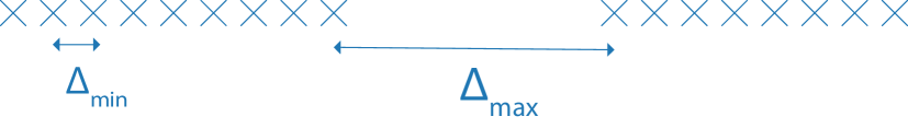
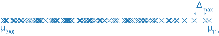
As illustration, consider a subset of images from the Chicago streetview dataset [17] shown in Fig. 1. In this study, people were asked to judge how safe each scene looks [18], and a larger mean indicates a safer looking scene. While each person has a different sense of how safe an image looks, when aggregated there are clear trends in the safety scores (denoted by ) of the images. Fig. 1 schematically shows the distribution of scores given by people as a bell curve below each image. Assuming the sample means are close to their true means, one can nominally classify them as ‘safe’, ‘maybe unsafe’ and ‘unsafe’ as indicated in Fig. 1. Here we have implicitly used the large gaps and to mark the boundaries. Note that finding the safest image (best-arm identification) is hard as we need a lot of human responses to decide the larger mean between the two rightmost distributions; it is also arguably unnecessary. A common way to address this problem is to specify a tolerance [7], and stop sampling if the means are less than apart; however determining this can require samples. Distinguishing the top distributions from the rest is easy and can be efficiently done using top- arm identification [15], however this requires the experimenter to prescribe the location where a large gap exists which is unknown. Automatically identifying natural splits in the set of distributions is the aim of the new theory and algorithms we propose. We call this problem of adaptive sampling to find the largest gap the MaxGap-bandit problem.
1.1 Notation and Problem Statement
We will use multi-armed bandit terminology and notation throughout the paper. The distributions will be called arms and drawing a sample from a distribution will be refered to as sampling the arm. Let denote the mean of the -th arm, . We add a parenthesis around the subscript to indicate the -th largest mean, i.e., . For the -th arm, we define its gap to be the maximum of its left and right gaps, i.e.,
| (1) |
We define and to account for the fact that extreme arms have only one gap. The goal of the MaxGap-bandit problem is to (adaptively) sample the arms and return two clusters
where is the rank of the arm with the largest gap between adjacent means, i.e.,
| (2) |
The mean values are unknown as is the ordering of the arms according to their means. A solution to the MaxGap-bandit problem is an algorithm which given a probability of error , samples the arms and upon stopping partitions into two clusters and such that
| (3) |
This setting is known as the fixed-confidence setting [10], and the goal is to achieve the probably correct clustering using as few samples as possible. In the sequel, we assume that is uniquely defined and let where .
1.2 Comparison to a Naive Algorithm: Sort then search for MaxGap
The MaxGap-bandit problem is not equivalent to best-arm identification on gaps since the MaxGap-bandit problem requires identifying the largest gap between adjacent arm means (best arm identification on gaps would always identify as the largest gap). This suggests a naive two-step algorithm: we first sample the arms enough number of times so as to identify all pairs of adjacent arms (i.e., we sort the arms according to their means), and then run a best-arm identification bandit algorithm [13] on the gaps between adjacent arms to identify the largest gap (an unbiased sample of the gap can be obtained by taking the difference of the samples of the two arms forming the gap).
We analyze the sample complexity of this naive algorithm in LABEL:sec:appendixsimple_algorithm , and discuss the results here for an example configuration. Consider the arrangement of means shown in Fig. 2 where there is one large gap and all the other gaps are equal to . The naive algorithm has a sample complexity (the first sorting step requires these many samples) which can be very large. Is this sorting of the arm means necessary? For instance, we do not need to sort real numbers in order to cluster them according to the largest gap.111First find the smallest and largest numbers, say and respectively. Divide the interval into equal-width bins and map each number to its corresponding bin, while maintaining the smallest and largest number in each bin. Since at least one bin is empty by the pigeonhole principle, the largest gap is between two numbers belonging to different bins. Calculate the gaps between the bins and report the largest as the answer. The algorithms we propose in this paper solve the MaxGap-bandit problem without necessarily sorting the arm means. For the configuration in Fig. 2 they require samples, giving a saving of approximately samples.
The analysis of our algorithms suggests a novel hardness parameter for the MaxGap-bandit problem that we discuss next. We let for all . We show in Section 5 that the number of samples taken from distribution due to its right gap is inversely proportional to the square of
| (4) |
For the left gap of we define analogously. The total number of samples drawn from distribution is inversely proportional to the square of . The intuition for Eq. 4 is that distribution can be eliminated quickly if there is another distribution that has a moderately large gap from (so that this gap can be quickly detected), but not too large (so that the gap is easy to distinguish from ), and (4) chooses the best . We discuss (4) in detail in Section 5, where we show that our algorithms use samples to find the largest gap with probability at least . This sample complexity is minimax optimal.
1.3 Summary of Main Results and Paper Organization
In addition to motivating and formulating the MaxGap-bandit problem, we make the following contributions. First, we design elimination and UCB-style algorithms as solutions to the MaxGap-bandit problem that do not require sorting the arm means (Section 3). These algorithms require computing upper bounds on the gaps , which can be formulated as a mixed integer optimization problem. We design a computationally efficient dynamic programming subroutine to solve this optimization problem and this is our second contribution (Section 4). Third, we analyze the sample complexity of our proposed algorithms, and discover a novel problem-hardness parameter (Section 5). This parameter arises because of the arm interactions in the MaxGap-bandit problem where, in order to reduce uncertainty in the value of an arm’s gap, we not only need to sample the said arm but also its neighboring arms. Fourth, we show that this sample complexity is minimax optimal (Section 6). Finally, we evaluate the empirical performance of our algorithms on simulated and real datasets and observe that they require x fewer samples than non-adaptive sampling to achieve the same error (Section 7).
2 Related Work
One line of related research is best-arm identification in multi-armed bandits. A typical goal in this setting is to identify the top- arms with largest means, where is a prespecified number [15, 16, 1, 3, 9, 4, 14, 7, 19]. As explained in Section 1, our motivation behind formulating the MaxGap-bandit problem is to have an adaptive algorithm which finds the “natural” set of top arms as delineated by the largest gap in consecutive mean values. Our work can also be used to automatically detect “outlier” arms [22].
The MaxGap-bandit problem is different from the standard multi-armed bandit because of the local dependence of an arm’s gap on other arms. Other best-arm settings where an arm’s reward can inform the quality of other arms include linear bandits [21] and combinatorial bandits [5, 11]. In these problems, the decision space is known to the learner, i.e., the vectors corresponding to the arms in linear bandits and the subsets of arms over which the objective function is to be optimized in combinatorial bandits is known to the learner. However in our problem, we do not know the sorted order of the arm means, i.e., the set of all valid gaps is unknown a priori. Our problem does not reduce to these settings.
Another related problem is noisy sorting and ranking. Here the typical goal is to sort a list using noisy pairwise comparisons. Our framework encompasses noisy ranking based on Borda scores [1]. The Borda score of an item is the probability that it is ranked higher in a pairwise comparison with another item chosen uniformly at random. In our setting, the Borda score is the mean of each distribution. Much of the theoretical computer science literature on this topic assumes a bounded noise model for comparisons (i.e., comparisons are probably correct with a positive margin) [8, 6, 2, 20]. This is unrealistic in many real-world applications since near equals or outright ties are not uncommon. The largest gap problem we study can be used to (partially) order items into two natural groups, one with large means and one with small means. Previous related work considered a similar problem with prescribed (non-adaptive) quantile groupings [18].
3 MaxGap Bandit Algorithms
We propose elimination [7] and UCB [13] style algorithms for the MaxGap-bandit problem. These algorithms operate on the arm gaps instead of the arm means. The subroutine to construct confidence intervals on the gaps (denoted by ) using confidence intervals on the arm means (denoted by ) is described in Algorithm 4 in Section 4, and this subroutine is used by all three algorithms described in this section.
3.1 Elimination Algorithm:
At each time step, (Algorithm 1) samples all arms in an active set consisting of arms whose gap upper bound is larger than the global lower bound on the maximum gap, and stops when there are only two arms in the active set.
3.2 UCB algorithms: and
(Algorithm 2) is motivated from the principle of “optimism in the face of uncertainty”. It samples all arms with the highest gap upper bound. Note that there are at least two arms with the highest gap upper bound because any gap is shared by at least two arms (one on the right and one on the left). The stopping condition is akin to the stopping condition in Jamieson et al. [13].
Alternatively, we can use an LUCB [16]-type algorithm that samples arms which have the two highest gap upper bounds, and stops when the second-largest gap upper bound is smaller than the global lower bound . We refer to this algorithm as (Algorithm 3).
4 Confidence Bounds for Gaps
In this section we explain how to construct confidence bounds for the arm gaps (denoted by and ) using confidence bounds for the arm means (denoted by ). These bounds are key ingredients for the algorithms described in Section 3.
Given i.i.d. samples from arm , an empirical mean and confidence interval on the arm mean can be constructed using standard methods. Let denote the number of samples from arm after time steps of the algorithm. Throughout our analysis and experimentation we use confidence intervals on the mean of the form
| (5) |
The confidence intervals are chosen so that [12]
| (6) |
Conceptually, the confidence intervals on the arm means can be used to construct upper confidence bounds on the mean gaps in the following manner. Consider all possible configurations of the arm means that satisfy the confidence interval constraints in (5). Each configuration fixes the gaps associated with any arm . Then the maximum gap value over all configurations is the upper confidence bound on arm ’s gap; we denote it as . The above procedure can be formulated as a mixed integer linear program (see Section B.1). In the algorithms in Section 3, this optimization problem needs to be solved at every time and for every arm before querying a new sample, which can be practically infeasible. In Algorithm 4, we give an efficient time dynamic programming algorithm to compute . We next explain the main ideas used in this algorithm, and refer the reader to Section B.2 for the proofs.
Each arm has a right and left gap, and , where is the rank of , i.e., . We construct separate upper bounds and for these gaps and then define . Here we provide an intuitive description for how the bounds are computed, focusing on as an example.
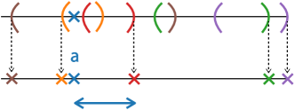
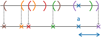
(a) (b)
To start, suppose the true mean of arm is known exactly, while the means of other arms are only known to lie within their confidence intervals. If there exist arms that cannot go to the left of arm , one can see that the largest right gap for is obtained by placing all arms that can go to the left of at their leftmost positions, and all remaining arms at their rightmost positions, as shown in Fig. 3(a). If however all arms can go to the left of arm , the configuration that gives the largest right gap for is obtained by placing the arm with the largest upper bound at its right boundary, and all other arms at their left boundaries, as illustrated in Fig. 3(b). We define a function that takes as input a known position for the mean of arm and the confidence intervals of all other arms at time , and returns the maximum right gap for arm using the above idea as follows.
| (7) |
However, the true mean of arm is not known exactly but only that it lies within its confidence interval. The insight that helps here is that must achieve its maximum when is at one of the finite locations in . We define as the set of arms pertinent to compute the right gap upper bound of , and then the maximum possible right gap of is
| (8) |
An upper bound for the left gap can be similarly obtained. We explain this and give a proof of correctness in LABEL:sec:appendix_gapucbalgorithm_proof.
The algorithms also use a single global lower bound on the maximum gap. To do so, we sort the items according to their empirical means, and find partitions of items that are clearly separated in terms of their confidence intervals. At time , let denote the arm with the -largest empirical mean, i.e., (this can be different from the true ranking which is denoted by without the subscript ). We detect a nonzero gap at arm if . Thus, a lower bound on the largest gap is
| (9) |
5 Analysis
In this section, we first state the accuracy and sample complexity guarantees for and , and then discuss our results. The proofs can be found in the Supplementary material.
Theorem 1.
With probability , , and cluster the arms according to the maximum gap, i.e., they satisfy (3).
The number of times arm is sampled by both the algorithms depends on a parameter where
| (10) | ||||
| (11) |
The maxima is assumed to be in (10) and (11) if there is no that satisfies the constraint to account for edge arms. The quantity acts as a measure of hardness for arm ; Theorem 2 states that and sample arm at most number of times (up to log factors).
Theorem 2.
With probability , the sample complexity of and is bounded by
Next, we provide intuition for why the sample complexity depends on the parameters in and (11). In particular, we show that (resp. ) is the number of samples of required to rule out arm ’s right (resp. left) gap from being the largest gap.
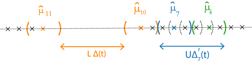
Let us focus on the right gap for simplicity. To understand how (10) naturally arises, consider Fig. 4, which denotes the confidence intervals on the means at some time . A lower bound on the gap can be computed between the left and right confidence bounds of arms and respectively as shown. Consider the computation of the upper bound on the right gap of arm . Arm lies to the right of arm with high probability (unlike the arms with dashed confidence intervals), so the upper bound . Considering only the right gap for simplicity, as soon as , arm can be eliminated as a candidate for the maximum gap.
Thus, an arm is removed from consideration as soon as we find a helper arm (arm in Fig. 4) that satisfies two properties: (1) the confidence interval of arm is disjoint from that of arm , and (2) the upper bound . The first of these conditions gives rise to the term in (10), and the second condition gives rise to the term . Since any arm that satisfies these conditions can act as a helper for arm , we take the maximum over all arms to yield the smallest sample complexity for arm .
This also shows that if all arms are either very close to or at a distance approximately from , then the upper bound and arm cannot be eliminated. Thus arm could have a small gap with respect to its adjacent arms, but if there is a large gap in the vicinity of arm , it cannot be eliminated quickly. This illustrates that the maximum gap identification problem is not equivalent to best-arm identification on gaps. Section 6 formalizes this intuition.
6 Minimax Lower Bound
In this section, we demonstrate that the MaxGap problem is fundamentally different from best-arm identification on gaps. We construct a problem instance and prove a lower bound on the number of samples needed by any probably correct algorithm. The lower bound matches the upper bounds in the previous section for this instance.
Lemma 1.
Consider a model with normal distributions , where
for some . Then any algorithm that is correct with probability at least must collect samples of arm in expectation.
Proof Outline: The proof uses a standard change of measure argument [10]. We construct another problem instance which has a different maximum gap clustering compared to (see Fig. 5; the maxgap clustering in is , while the maxgap clustering in is ), and show that in order to distinguish between and , any probably correct algorithm must collect at least samples of arm in expectation (see LABEL:sec:appendix_lowerbound for details).
From the definition of using (10),(11), it is easy to check that . Therefore, for problem instance our algorithms find the maxgap clustering using at most samples of arm (c.f. Theorem 2). This essentially matches the lower bound above.
This example illustrates why the maximum gap identification problem is different from a simple best-arm identification on gaps. Suppose an oracle told a best-arm identification algorithm the ordering of the arm means. Using the ordering it can convert the -arm maximum gap problem to a best arm identification problem on gaps, with distributions , and . The best-arm algorithm can sample arms and to get a sample of the gap . We know from standard best-arm identification analysis [13] that the gap can be eliminated from being the largest by sampling it (and hence arm ) times, which can be arbitrarily lower than the lower bound in Lemma 1. Thus the ordering information given to the best-arm identification algorithm is crucial for it to quickly identify the larger gaps. The problem we solve in this paper is identifying the maximum gap when the ordering information is not available.
7 Experiments
7.1 Streetview Dataset
(a)
(b)
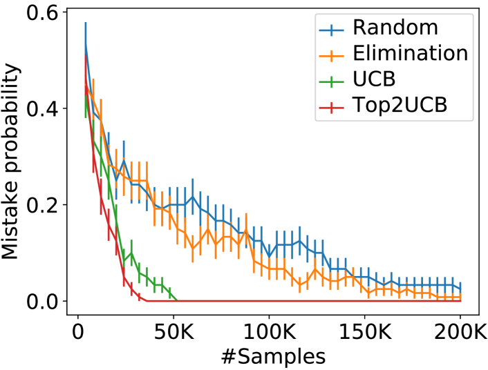
In our first experiment we study performance on the Streetview dataset [17, 18] whose means are plotted in Fig. 6(a) . We have arms, where each arm is a normal distribution with mean equal to the Borda safety score of the image and standard deviation . The largest gap of is between arms and , and the second largest gap is . In Fig. 6(b), we plot the fraction of times in runs as a function of the number of samples, for four algorithms, viz., random (non-adaptive) sampling, , , and . The error bars denote standard deviation over the runs. and require x fewer samples than random sampling.
7.2 Simulated Data
(a)
(b)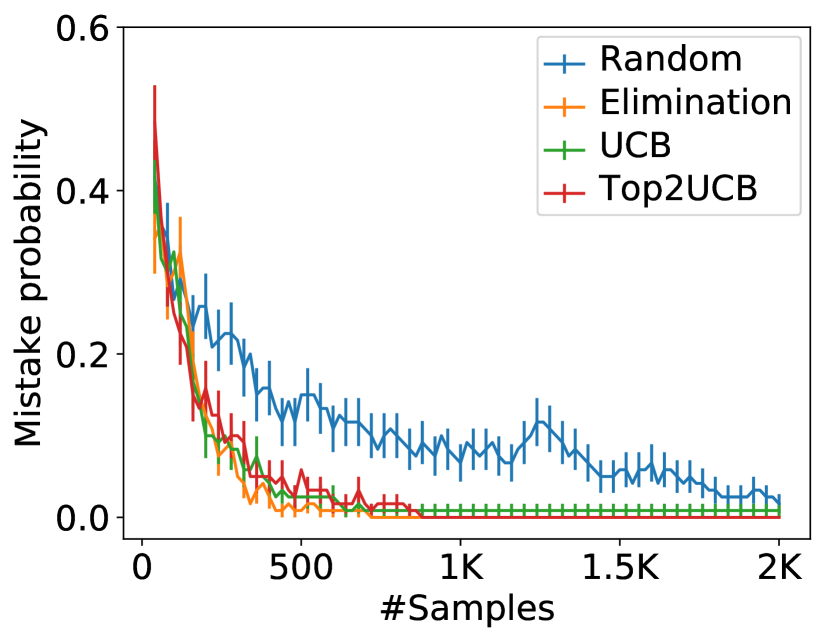
(c)
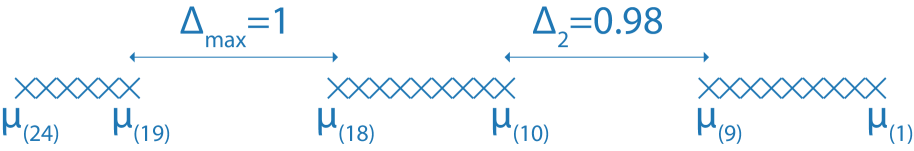
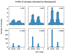
In the second experiment, we study the performance on on a simulated set of means containing two large gaps. The mean distribution plotted in LABEL:fig:simulatedexperiment(a) has arms (), with two large mean gaps , and remaining small gaps ( for ). We expect to see a big advantage for adaptive sampling in this example because almost every sub-optimal arm has a helper arm (see Section 5) which can help eliminate it quickly, and adaptive algorithms can then focus on distinguishing the two large gaps. A non-adaptive algorithm on the other hand would continue sampling all arms. We plot the fraction of times in runs in Fig. 7(b), and see that the active algorithms identify the largest gap in 8x fewer samples. To visualize the adaptive allocation of samples to the arms, we plot in Fig. 7(c) the number of samples queried for each arm at different time steps by MaxGapUCB. Initially, MaxGapUCB allocates samples uniformly over all the arms. After a few time steps, we see a bi-modal profile in the number of samples. Since all arms that achieve the largest are sampled, we see that several arms that are near the pairs and are also sampled frequently. As time progresses, only the pairs and get sampled, and eventually more samples are allocated to the larger gap among the two.
8 Conclusion
In this paper, we proposed the MaxGap-bandit problem: a novel maximum-gap identification problem that can be used as a basic primitive for clustering and approximate ranking. Our analysis shows a novel hardness parameter for the problem, and our experiments show 6-8x gains compared to non-adaptive algorithms. We use simple Hoeffding based confidence intervals in our analysis for simplicity, but better bounds can be obtained using tighter confidence intervals [13].
References
- Agarwal et al. [2017] Arpit Agarwal, Shivani Agarwal, Sepehr Assadi, and Sanjeev Khanna. Learning with limited rounds of adaptivity: Coin tossing, multi-armed bandits, and ranking from pairwise comparisons. In Conference on Learning Theory, pages 39–75, 2017.
- Braverman et al. [2016] Mark Braverman, Jieming Mao, and S Matthew Weinberg. Parallel algorithms for select and partition with noisy comparisons. In Proceedings of the forty-eighth annual ACM symposium on Theory of Computing, pages 851–862. ACM, 2016.
- Bubeck et al. [2013] Sebastien Bubeck, Tengyao Wang, and Nitin Viswanathan. Multiple identifications in multi-armed bandits. In Proceedings of the 30th International Conference on International Conference on Machine Learning - Volume 28, ICML’13, pages I–258–I–265. JMLR.org, 2013. URL http://dl.acm.org/citation.cfm?id=3042817.3042848.
- Chen et al. [2017] Lijie Chen, Jian Li, and Mingda Qiao. Nearly instance optimal sample complexity bounds for top-k arm selection. In Artificial Intelligence and Statistics, pages 101–110, 2017.
- Chen et al. [2014] Shouyuan Chen, Tian Lin, Irwin King, Michael R Lyu, and Wei Chen. Combinatorial pure exploration of multi-armed bandits. In Z. Ghahramani, M. Welling, C. Cortes, N. D. Lawrence, and K. Q. Weinberger, editors, Advances in Neural Information Processing Systems 27, pages 379–387. Curran Associates, Inc., 2014. URL http://papers.nips.cc/paper/5433-combinatorial-pure-exploration-of-multi-armed-bandits.pdf.
- Davidson et al. [2014] Susan Davidson, Sanjeev Khanna, Tova Milo, and Sudeepa Roy. Top-k and clustering with noisy comparisons. ACM Transactions on Database Systems (TODS), 39(4):35, 2014.
- Even-Dar et al. [2006] Eyal Even-Dar, Shie Mannor, and Yishay Mansour. Action elimination and stopping conditions for the multi-armed bandit and reinforcement learning problems. Journal of machine learning research, 7(Jun):1079–1105, 2006.
- Feige et al. [1994] Uriel Feige, Prabhakar Raghavan, David Peleg, and Eli Upfal. Computing with noisy information. SIAM Journal on Computing, 23(5):1001–1018, 1994.
- Gabillon et al. [2012] Victor Gabillon, Mohammad Ghavamzadeh, and Alessandro Lazaric. Best arm identification: A unified approach to fixed budget and fixed confidence. In Advances in Neural Information Processing Systems, pages 3212–3220, 2012.
- Garivier and Kaufmann [2016] Aurélien Garivier and Emilie Kaufmann. Optimal best arm identification with fixed confidence. In Conference on Learning Theory, pages 998–1027, 2016.
- Huang et al. [2018] Weiran Huang, Jungseul Ok, Liang Li, and Wei Chen. Combinatorial pure exploration with continuous and separable reward functions and its applications. In IJCAI, volume 18, pages 2291–2297, 2018.
- Jamieson and Nowak [2014] Kevin Jamieson and Robert Nowak. Best-arm identification algorithms for multi-armed bandits in the fixed confidence setting. In 2014 48th Annual Conference on Information Sciences and Systems (CISS), pages 1–6. IEEE, 2014.
- Jamieson et al. [2014] Kevin Jamieson, Matthew Malloy, Robert Nowak, and Sébastien Bubeck. lil’ucb: An optimal exploration algorithm for multi-armed bandits. In Conference on Learning Theory, pages 423–439, 2014.
- Jun et al. [2016] Kwang-Sung Jun, Kevin G Jamieson, Robert D Nowak, and Xiaojin Zhu. Top arm identification in multi-armed bandits with batch arm pulls. In AISTATS, pages 139–148, 2016.
- Kalyanakrishnan and Stone [2010] Shivaram Kalyanakrishnan and Peter Stone. Efficient selection of multiple bandit arms: Theory and practice. In ICML, volume 10, pages 511–518, 2010.
- Kalyanakrishnan et al. [2012] Shivaram Kalyanakrishnan, Ambuj Tewari, Peter Auer, and Peter Stone. Pac subset selection in stochastic multi-armed bandits. In ICML, volume 12, pages 655–662, 2012.
- Katariya et al. [2018a] Sumeet Katariya, Lalit Jain, Nandana Sengupta, James Evans, and Robert Nowak. Chicago streetview dataset. 2018a. URL https://github.com/sumeetsk/coarse_ranking/.
- Katariya et al. [2018b] Sumeet Katariya, Lalit Jain, Nandana Sengupta, James Evans, and Robert Nowak. Adaptive sampling for coarse ranking. In International Conference on Artificial Intelligence and Statistics, pages 1839–1848, 2018b.
- Mannor and Tsitsiklis [2004] Shie Mannor and John N Tsitsiklis. The sample complexity of exploration in the multi-armed bandit problem. Journal of Machine Learning Research, 5(Jun):623–648, 2004.
- Mao et al. [2018] Cheng Mao, Jonathan Weed, and Philippe Rigollet. Minimax rates and efficient algorithms for noisy sorting. In Firdaus Janoos, Mehryar Mohri, and Karthik Sridharan, editors, Proceedings of Algorithmic Learning Theory, volume 83 of Proceedings of Machine Learning Research, pages 821–847. PMLR, 07–09 Apr 2018. URL http://proceedings.mlr.press/v83/mao18a.html.
- Soare et al. [2014] Marta Soare, Alessandro Lazaric, and Rémi Munos. Best-arm identification in linear bandits. In Advances in Neural Information Processing Systems, pages 828–836, 2014.
- Zhuang et al. [2017] Honglei Zhuang, Chi Wang, and Yifan Wang. Identifying outlier arms in multi-armed bandit. In Advances in Neural Information Processing Systems, pages 5204–5213, 2017.
Appendix A Details for Section 1.2: Comparison to a Naive Algorithm
The naive algorithm first sorts the arms to determine the adjacent arms for every arm, and then runs a best-arm identification bandit algorithm on the gaps to identify the largest gap. An unbiased sample of the gap between two arms can be obtained by taking the difference of the samples from the two arms. Here we analyze the sample complexity of the naive algorithm for a general arrangement of the means.
Consider an arm , and let us analyze the number of times arm is sampled by the naive algorithm. Let . Then is the right gap of arm ( is defined analogously). In the first step of the naive algorithm, arm needs to be sampled at least times to determine its right neighbor. Once the right neighbor has been determined, the best-arm identification requires at least samples to distinguish arm ’s right gap from . Since samples from the first step can be reused, the minimum number of samples required by the naive algorithm to rule out arm ’s right gap is where
| (12) |
We can define analogously, and the naive algorithm collects from arm , where .
The hardness parameter of our active algorithms that is analogous to (12) is given by (4), repeated here for convenience
| (13) |
For the toy problem discussed in Section 1.2, if we assume that , we have that , while , which results in order savings in the number of samples.
Appendix B Details for Section 4: Confidence Bounds for Gaps
We first explain the mixed integer program formulation for obtaining the upper confidence bounds on the mean gaps in Section B.1, and then prove the validity of Algorithm 4 in LABEL:sec:appendix_gapucb_algorithmproof.
B.1 MIP Formulation of Confidence Bounds for Gaps
Conceptually, the confidence intervals on the arm means can be used to construct upper confidence bounds on the mean gaps in the following manner. Consider all possible configurations of the arm means that satisfy the confidence interval constraints in (5). Each configuration fixes the gaps associated with any arm . Then the maximum gap value over all configurations is the upper confidence bound on arm ’s gap; we denote it as .
If we focus on the right gap of arm , the above procedure is equivalent to solving the following optimization problem.
| (14) | ||||
| (15) | ||||
| (16) |
Constraint (15) ensures that is in the confidence interval for the mean of arm at time , and constraint (16) ensures that arm is the right neighbor of arm .
The constraint (16) is a sorting constraint that can only be formulated using a binary variable. For an arm (16) can be formulated using a constant as
| (17a) | ||||
| (17b) | ||||
| (17c) | ||||
The value of is chosen to be large number. Replacing constraint (16) by constraints (17a), (17b), (17c) for all gives an equivalent optimization problem whose optimum value is . This can be seen to be true by considering the cases based on the value of . If and if . Because is chosen to be a large number, in either case and constraint (16) is satisfied. If constraint (16) is satisfied, then a similar argument allows us to choose the value of that satisfies constraints (17a) and (17b).
B.2 Validity of Algorithm 4
In this section we find the value of as defined in (14) by first obtaining an upper bound to it. The proof of the upper bound is constructive in nature, showing that the upper bound is actually achievable. That is, (a) there is a set of real numbers which satisfy (15), (b) an index which satisfies (16) with , such that .
We first find an upper bound to the right gap of an arm assuming we know its true mean , but only have confidence intervals for the means of the other arms .
Lemma 2.
If all the arm means are known, the right gap associated with an arm is ; if the domain is empty we say that arm ’s right gap is . For any , define a function of the confidence intervals as follows.
Suppose we know the value of arm ’s mean, i.e. and the confidence intervals . Then the largest possible right gap of arm is .
Proof.
We suppose that the right gap of arm is greater than the upper bound and show a contradiction to the good event (6).
Case I: . Identify the arm such that . Let the true right gap for arm be . If , then would mean that , which is a contradiction. If and the right gap is , then all arms are such that . But if then , and from the domain in the definition of , its left bound . Hence the confidence interval of satisfies . If then and that is a contradiction.
Case II: . Identify the arm such that . Let the true right gap for arm be . If then and that is a contradiction.
Thus the right gap of arm is at most . We can achieve this upper bound by choosing the set of means in the following manner. If the value of is given by the first branch, set and . Otherwise if the value is given by the second branch set for the arm which has the largest right bound, and set all other (c.f. Fig. 3 in Section 4).∎
The left gap analog of the above proposition can also be proved in a similar manner as above.
Lemma 3.
For any and arm , define a function of the confidence intervals as follows.
| (18) |
Suppose we know . Using the confidence intervals , an upper bound to the left gap of arm is .
We now replace our knowledge of the true mean value by the good event fact that at all times . The following lemma is instrumental in arriving at an upper bound for the right gap of arm that is consistent with the all the arms’ confidence intervals.
Lemma 4.
At time , for any arm its true mean in the good event. Define a subset of arms whose left bounds lie within the confidence interval of arm . Consider a set of real numbers , each associated with a corresponding arm. The largest value for the right gap of arm if the means are , i.e.,
occurs when for some .
Proof.
Suppose the largest right gap occurs when for any . Note that and hence the set is not empty. We show that the right gap can be larger while still satisfying event (6). Let . Collect all arms in the set . Consider an alternate bandit model whose arm means are denoted by . We assign
This mean assignment satisfies . This is because by definition of arm in the original bandit model , for all arms their left bounds satisfy . Thus both the original and the alternate are possible bandit models in the good event (6) up till current time . However, the right gap for is larger in the alternate model as shown next. Let arm result in the right gap for in the original model , i.e., the right gap is
Then in the alternate model, and there is no mean . Then the right gap of arm is . This contradicts the supposition that the right gap is the largest possible in the original bandit model . ∎
An analogous lemma for the left gap states that for any set of possible arm means that are consistent with the current confidence intervals, the largest possible left gap of arm occurs when for some arm . Using the above, we can state the upper bound for the gap of an arm in terms of all the confidence intervals as follows.
Theorem 3.
At any time , denote the upper bound to the right (resp. left) gap of arm by (resp. ). The expressions for these upper bounds in terms of the confidence intervals and the functions in Lemma 2, Lemma 3 are as follows.
| (19) |
Then an upper bound to the gap associated with arm at time is . Algorithm 4 gives pseudocode that evaluates .
Proof.
We argue for the right gap, an analogous proof gives the statement for the left gap. At any time in the good event , in particular any number in the range can be potentially the mean of arm . From Lemma 4, we know that for a set of numbers that satisfy all current confidence intervals and also maximize the right gap for arm , the value for some left bound . If then by Lemma 2 is the largest possible value for arm in the bandit model . Taking the maximum over all arms in the set , we get the right gap upper bound .
We note that the value is achievable by an assignment of means that satisfy the confidence bounds at time . Without loss of generality, assume for some arm . One can assign and other means in a way similar to that in the proof of Lemma 2 to obtain a right gap for arm equal to the value . ∎
Appendix C Details for Section 5: Accuracy
See 1
Proof.
Recall that the true maximum gap exists between arms and . The algorithms return a wrong clustering for any time . We show that this leads to a contradiction if the good event (6) holds.
Assume (6) holds and at some time . Recall that is computed using , and let be the maximizer in (9). Let be such that and . If holds, we have that
where (a) holds because is the minimum gap between a left confidence interval in and a right confidence interval in . This contradicts the fact that is the largest gap. ∎
Appendix D Sample Complexity: Proof of Theorem 2
To state our sample complexity bounds we use a constant defined as follows [7].
Remark 1.
There exists constant such that for all , if the number of samples , then , where is the confidence interval given by (5).
D.1 Sample Complexity of
Early Stopping Rule for Clustering: In the pseudocode in Algorithm 1, stops when the size of the active set (line ). However, if we are only interested in clustering the arms according to the maximum gap and not interested in the identities of the arms which share the maximum gap (arms ), we can stop earlier as follows. Assume that (9) is greater than 0 and let be the maximizer. This partitions the arms into the sets and . can terminate when the maximum left gap of all arms in and the maximum right gap of all arms in are both less than the lower bound . The termination condition can be expressed as , where
| (20) |
To account for the lower sample complexity as a result of the stopping rule for clustering, we modify (10) and (11) and define new parameters that yield an improved sample complexity than that stated in Theorem 2. Define
| (21) | |||||
| (22) |
where just like in (10), the maxima assumed to be infinity if there is no that satisfies the constraint under the inner maximization. We define as before and state our improved sample complexity bound for next.
Theorem 4.
With probability at least , the sample complexity of is bounded by
Proof.
Lemma 5.
Proof.
Lemma 6.
Assume (6) holds, and consider . In MaxGapElim if is such that , then
Proof.
Note that at time in Algorithm 1, and for all arms . Assume (6) holds. We have . This implies that
| (23) |
where (a) holds by Lemma 5.
From (23) we have that
| (24) |
Recall from (21) that for ,
| (25) |
There are two terms in and could be less than either of these terms. First, suppose that
and let
| (26) |
For any arm such that , the inner minimum in (26) will be negative. On the other hand, since , there must exist an arm such that , and for such an arm the inner minimum will be positive. Since is the arm that maximizes the inner minimum, the inner minimum must be positive for . Thus we have that .
Lemma 7.
Assume (6) holds, and consider . In MaxGapElim if is such that , then
Proof.
The proof is analogous to the proof of Lemma 6. ∎
D.2 Sample Complexity of
For the sample complexity analysis of MaxGapUCB , we use a modified version of the left and right confidence bounds introduced in (5). We redefine
| (28) |
The nice property that these bounds have is that for all . Lemma 9 shows that these modified bounds retain the same confidence guarantee for the arm mean values as the original confidence bounds. In what follows, we will exclusively use the modified confidence bounds (except in Lemma 9 where we show they are correct). We drop the prime symbol in their notation for brevity and henceforth denote the modified confidence bounds given in (28).
We state and prove our main sample complexity result in Theorem 5.
Theorem 5.
With probability at least , the number of times samples a sub-optimal arm, i.e. an arm , is upper bounded by . The constant is defined in Remark 1. Thus, the number of times samples suboptimal arms is
Proof.
We show that the result holds true as long as the confidence intervals for the means are correct (6). Let
| (29) |
where is defined in LABEL:remark:confidence_interval_samplecomplexity. Note that . Arm is sampled either because is the largest or is the largest. We prove in LABEL:lem:ucbrightgap_lessthan_deltamax below that when is sampled times due to its right gap, . Hence will not sample due to its right gap more than times because beyond this point will be higher. It can similarly be proved that when is sampled times due to its left gap, . Thus, arm will be sampled at most times. ∎
To ease the explanation, we only focus on the right gap of from here onwards and set
| (30) |
Furthermore, in the lemmas below, we only focus on samples of drawn when was the largest upper bound. With a slight overload of notation, let denote the (random) smallest time when arm has been sampled times by (owing to its right gap).
Lemma 8.
With probability ,
Proof.
Since the proof is long and technical, we first give an outline of the entire proof.
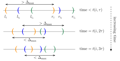
Outline: Define and to be the arms that form the left and right boundaries of (the two arms that result in the maximum value of (8) at ). By this definition, . Consider the arms used in computing , i.e. , and denote them as for brevity. Fig. 8 shows the confidence intervals of in blue and those of in green. Initially the confidence intervals are large, i.e., the width between the right and left bounds of arm is greater than before time . After rounds of , the confidence interval of will have shrunk. However, note that the right gap of arm involves either and/or . Since samples all arms that can attain the highest gap upper bound, it turns out that it will also sample enough times to make . If is still sampled after rounds due to its right gap, then its gap upper bound must involve an arm which is disjoint from ’s confidence interval, such as the arm . Then from to , samples and enough times to make .
We divide the proof into four parts. In the first part, we divide all the arms into subsets (which we refer to as levels). These subsets are defined such that arms within a subset obey collective properties, that we study in some of the subsequent lemmascolor=Chocolate1,size=,]S: lemmas section. In the second and third part, we prove that arms and are always sampled whenever is sampled from . Finally in part four, we use these arms to argue that .
Level Sets:
At any time , we can identify three subsets of arms with respect to arm that we refer to as level , level , and level arms respectively, and argue that the arms that define must lie in one of these subsets. These levels sets are defined as follows. Let
| (31) | ||||
| (32) | ||||
| (33) |
From their definitions the three subsets are pairwise disjoint at every . Let
| (34) |
denote the union of the three levels. From the definition of in (8) and (31), (32), the arm
| (35) |
Lemma 10 proves that the arm . Thus at any time , only arms in are relevant for the right gap of arm .
color=Chocolate1,size=,]S: move proof of also to Lemma 11?
Suppose , i.e., arm is sampled at least times. To avoid clutter,we let
and use the full notation for . We next argue that and must be sampled times before .
must have been sampled at least times before :
By Lemma 10, . From Corollary 2, . If for any , then by Lemma 9 and Lemma 11, and we are done. Let us hence look at the case when . We have by Lemma 11 that , and Lemma 13 then implies that must be sampled whenever was sampled for . Hence is sampled at least times before .
must have been sampled at least times before :
From Corollary 2, since the level of an arm cannot decrease from 2 to 1, color=Chocolate1,size=,]S: lemma that says level cannot decrease from 2 missing? A; Cor 2 gives it? for all . If , then is sampled times whenever is sampled by Lemma 13.
On the other hand, if for some , let . We consider two cases, and . First, if , then for all by Lemma 9. Since , we have by Lemma 9 and Lemma 11 that
| (36) |
By the definition of in (8) we have that
| (37) |
(37) and (36) imply that , and we are done. For the second case, suppose . Lemma 12 then gives that arm is also sampled at time . Thus, we have shown that either , or is sampled whenever is sampled in .
We now show that .
:
Recall that are all larger than .
Let
be the maximizer in (10), and note that by definition. Also note that and are defined in (30) and (10) respectively so that
| (38) |
We split the proof into various cases depending on the ordering of the means . First, note that if , then
by (38). Second, if , then
by (38). Third, we show that it cannot be the case that . Assume to the contrary. This implies that
which contradicts Eq. 35. Fourth, it cannot be the case that , because by Lemma 11. The only case that remains is , which we prove next by showing that .
color=Chocolate1,size=,]S: confirm that we haven’t assume anywhere in the proof
:
For any time such that , we have by Lemma 11 and Lemma 13 that is sampled whenever is sampled. Thus we only need to focus on times when .
Suppose now that for some when was sampled and . Recall that . We consider two cases depending on whether or .
- •
- •
This proves that . We use this to prove that as follows. First note that color=Chocolate1,size=,]S: add discussion somewhere about why has been chosen this way
Second, since arm , and hence
Hence
∎
Lemma 9.
Over the sigma-algebra generated by all the arm rewards up till any time , we have that
| (39) |
Proof.
Let be the event in the LHS of (39) and let be the good event. First we show that . The event implies that at any time and for any arm , we have that
Hence the good event is true in this case.
Now we show that . Suppose that is not true, so there is a time and arm such that . Choose two time instants such that . Then the supposition implies that either
Either of the above statements imply that the good event is not true. Hence . ∎
Corollary 1.
For any two time instants if then .
Proof.
Corollary 2.
For all if then at all time instants . If then at all .
Proof.
Define . For any , if then using Lemma 9,
| (40) |
Hence if , from (33) we have that and we get
where the inequality (a) is true because of Lemma 9 and inequality (b) is true as by (40). This implies that .
If we have that . At any , from Lemma 9 we have that , i.e., the arm . ∎
Proof.
Suppose arm , then either which would give a negative value for , or we have that . From the definition of arm , its . Using this and (7), we have that
| (41) |
From the definition of arm , we have that as argued above. That implies , which contradicts the supposition. ∎
Lemma 11.
At any time , all arms are such that .
Proof.
Consider an arm , then for all for otherwise that would contradict corollary 2. Thus for all .
By choice of we have that from (38). Hence if arm for any , we have that , where inequality (a) is by Lemma 9.
Hence for all . If is the largest gap upper bound then by the above reasoning. Then Lemma 13 states that arm was sampled anytime arm was sampled between to . This implies that , and we argue that in the following manner. The arm is the maximizer in (10).
Case I: . Here we argue that because as shown below.
Case II: . Here we argue that as shown below.
∎
Lemma 12.
Suppose arm is sampled at time because is the largest gap upper bound. Consider an arm whose confidence bounds satisfy any one of the following conditions.
-
1.
, or
-
2.
.
Then MaxGapUCB samples arm as well at time .
Proof.
Suppose arm satisfies condition (1). Consider the right gap of arm , we have that . If the value of is obtained by the first branch of (7), then the value of is also given by its first branch. That implies , and hence is sampled if is sampled. If , by condition (1) we have that , which implies that is obtained by the second branch in (7). Hence for all arms we have and . Considering the left gap of arm , since ,
and arm is sampled if is sampled. Finally suppose the value of is obtained by the second branch in (7), and . Then
where the last equality is true because if not, then , which contradicts the condition that is the largest. Hence arm is sampled if is sampled.
Suppose now that arm satisfies condition (2). We divide the proof of this part into two cases.
Case I: Suppose .
If the arm , then we show that cannot be the largest gap upper bound. Consider the arm , it satisfies . Then , where the first branch of (7) is active because of arm . But
That would imply
which contradicts the identification of arm as the one giving the value of . The case that remains is if the arm . For this part consider the following two sub-cases:
Sub-case Ia: The set of arms . Since the number of arms , the value , and hence if , then it must be due to the first branch in (7). That implies . Then consider the left gap for arm that satisfies condition (2). Since the set , we have
which implies that arm will be sampled if is the largest.
Sub-case Ib: The set of arms . Consider the arm , the domain in the maximization is not empty because of the following. By the case assumption, there is an arm whose . If the left bound of this arm , then , which contradicts the identification of arm for . Hence its left bound must satisfy . Now consider the right gap of arm defined above. Since , we have that . But
which implies that , which is a contradiction. We are left with the following Case II.
Case II: Suppose .
Let be such that . Then . If the previous inequality is strict, then we have that
which contradicts the identification of arm as the one giving the value of . Hence we have that
and arm is sampled if arm is sampled because of . ∎
Lemma 13.
Suppose arm is sampled at time when . If then all arms in the set are sampled by MaxGapUCB. If then all arms in the set are sampled by MaxGapUCB. color=Chocolate1,size=,]S: break into 2 lemmas? one for level 1 and one for level 2
Proof.
The qualifying condition states that the arm , hence from definitions (32), (33) we have that . By definition (8) the arm is such that . We first argue that all arms in the set are sampled. For arm . If , arm satisfies condition (1) of Lemma 12 and hence is sampled if is the largest. If on the other hand , then arm satisfies condition (2) of Lemma 12 and hence it is sampled if is sampled. The remaining case is if , but that would contradict the identification of the arm for .
Now suppose arm , what is left to prove is that all arms in the set are sampled. Since , we have that
where the last equality is true because arm satisfies . From definition (33), any is such that and satisfies condition (2) of Lemma 12. Hence arm is sampled if is sampled because of its right gap. ∎
Appendix E Details for Section 6: Proof of Lemma 1
See 1
Proof.
The maximum gap in is . Define an alternate bandit model with normal distributions where
Note that the ordering of the means in does not follow the subscript indices, indeed . The two measures are illustrated in Fig. 9. The maximum gap in is and is no longer a valid gap between consecutive arms. Consider algorithm for identifying the maximum gap and let denote the top-cluster returned by the algorithm when it stops at time . Let . Assume that and . Letting denote the binary relative entropy, Lemma 1 in Garivier and Kaufmann [10] implies that
Similarly, one can show that by creating an alternative bandit instance identical to except . ∎