Abstract

We introduce the problem of model selection for contextual bandits, where a learner must adapt to the complexity of the optimal policy while balancing exploration and exploitation. Our main result is a new model selection guarantee for linear contextual bandits. We work in the stochastic realizable setting with a sequence of nested linear policy classes of dimension $d_{1}<d_{2}<\ldots$, where the $m^{\star}$-th class contains the optimal policy, and we design an algorithm that achieves $\tilde{O}(T^{2/3}d^{1/3}_{m^{\star}})$ regret with no prior knowledge of the optimal dimension $d_{m^{\star}}$. The algorithm also achieves regret $\tilde{O}\left(T^{3/4}+\sqrt{Td_{m^{\star}}}\right)$, which is optimal for $d_{m^{\star}}\geq{}\sqrt{T}$. This is the first contextual bandit model selection result with non-vacuous regret for all values of $d_{m^{\star}}$, and to the best of our knowledge is the first positive result of this type for any online learning setting with partial information. The core of the algorithm is a new estimator for the gap in the best loss achievable by two linear policy classes, which we show admits a convergence rate faster than the rate required to learn the parameters for either class.

1 Introduction

Model selection is the fundamental statistical task of choosing a hypothesis class using data. The choice of hypothesis class modulates a tradeoff between approximation error and estimation error, as a small class can be learned with less data, but may have worse asymptotic performance than a richer class. In the classical statistical learning setting, model selection algorithms provide the following luckiness guarantee: If the class of models decomposes as a nested sequence $\mathcal{F}_{1}\subset\mathcal{F}_{2}\subset\cdots\mathcal{F}_{m}\subset\mathcal{F}$, the sample complexity of the algorithm scales with the statistical complexity of the smallest subclass $\mathcal{F}_{m^{\star}}$ containing the true model, even though $m^{\star}$ is not known in advance. Such guarantees date back to Vapnik’s structural risk minimization principle and are by now well-known (Vapnik, 1982, 1992; Devroye et al., 1996; Birgé and Massart, 1998; Shawe-Taylor et al., 1998; Lugosi and Nobel, 1999; Koltchinskii, 2001; Bartlett et al., 2002; Massart, 2007). In practice, one may use cross-validation—the de-facto model selection procedure—to decide whether to use, for example, a linear model, a decision tree, or a neural network. That cross-validation appears in virtually every machine learning pipeline highlights the necessity of model selection for successful ML deployments.

We investigate model selection in contextual bandits, a simple interactive learning setting. Our main question is: Can model selection guarantees be achieved in contextual bandit learning, where a learner must balance exploration and exploitation to make decisions online?

Contextual bandit learning is more challenging than statistical learning on two fronts: First, decisions must be made online without seeing the entire dataset, and second, the learner’s actions influence what data is observed (“bandit feedback”). Between these extremes is full-information online learning, where the learner does not have to deal with bandit feedback, but still makes decisions online. Even in this simpler setting, model selection is challenging, since the learner must attempt to identify the appropriate model class while making irrevocable decisions and incurring regret. Nevertheless, several prior works on so-called parameter-free online learning (McMahan and Abernethy, 2013; Orabona, 2014; Koolen and Van Erven, 2015; Luo and Schapire, 2015; Foster et al., 2017; Cutkosky and Boahen, 2017) provide algorithms for online model selection with guarantees analogous to those in statistical learning. With bandit feedback, however, the learner must carefully balance exploration and exploitation, which presents a substantial challenge for model selection. At an intuitive level, the reason is that different hypothesis classes require different amounts of exploration, but either over- or under-exploring can incur significant regret (A detailed discussion requires a formal setup and is deferred to Section 2). At this point, it suffices to say that prior to this work, we are not aware of any adequate model selection guarantee that adapts results from statistical learning to any online learning setting with partial information.

We provide a new model selection guarantee for the linear stochastic contextual bandit setting (Chu et al., 2011; Abbasi-Yadkori et al., 2011). We consider a sequence of feature maps into $d_{1}<d_{2}<\ldots<d_{M}$ dimensions and assume that the losses are linearly related to the contexts via the $m^{\star}$-th feature map, so that the optimal policy is a $d_{m^{\star}}$-dimensional linear policy. We design an algorithm that achieves $\tilde{O}(T^{2/3}d^{1/3}_{m^{\star}})$ regret to this optimal policy over $T$ rounds, with no prior knowledge of $d_{m^{\star}}$. As this bound has no dependence on the maximum dimensionality $d_{M}$, we say that the algorithm adapts to the complexity of the optimal policy. All prior approaches suffer linear regret for non-trivial values of $d_{m^{\star}}$, whereas the regret of our algorithm is sublinear whenever $d_{m^{\star}}$ is such that the problem is learnable. Our algorithm can also be tuned to achieve $\tilde{O}\left(T^{3/4}+\sqrt{Td_{m^{\star}}}\right)$ regret, which matches the optimal rate when $d_{m^{\star}}\geq{}\sqrt{T}$.

At a technical level, we design a sequential test to determine whether the optimal square loss for a large linear class is substantially better than that of a smaller linear class. We show that this test has sublinear sample complexity: while learning a near-optimal predictor in $d$ dimensions requires at least $\Omega(d)$ labeled examples, we can estimate the improvement in value of the optimal loss using only $O(\sqrt{d})$ examples, analogous to so-called variance estimation results in statistics (Dicker, 2014; Kong and Valiant, 2018). Crucially, this implies that we can test whether or not to use the larger class without over-exploring for the smaller class.

2 Preliminaries

We work in the stochastic contextual bandit setting (Langford and Zhang, 2008; Beygelzimer et al., 2011; Agarwal et al., 2014). The setting is defined by a context space $\mathcal{X}$, a finite action space $\mathcal{A}\vcentcolon=\{1,\ldots,K\}$ and a distribution $\mathcal{D}$ supported over $(x,\ell)$ pairs, where $x\in\mathcal{X}$ and $\ell\in\mathbb{R}^{\mathcal{A}}$ is a loss vector. The learner interacts with nature for $T$ rounds, where in round $t$: (1) nature samples $(x_{t},\ell_{t})\sim\mathcal{D}$, (2) the learner observes $x_{t}$ and chooses action $a_{t}$, (3) the learner observes $\ell_{t}(a_{t})$. The goal of the learner is to choose actions to minimize the cumulative loss.

Following several prior works (Chu et al., 2011; Abbasi-Yadkori et al., 2011; Agarwal et al., 2012; Russo and Van Roy, 2013; Li et al., 2017), we study a variant of the contextual bandit setting where the learner has access to a class of regression functions $\mathcal{F}:\mathcal{X}\times\mathcal{A}\to\mathbb{R}$ containing the Bayes optimal regressor

$$f^{\star}(x,a)\vcentcolon=\mathbb{E}\left[\ell(a)\mid x\right]\quad\forall x,a.$$ (1)

We refer to this assumption ($f^{\star}\in\mathcal{F}$) as realizability. For each regression function $f$ we define the induced policy $\pi_{f}(x)\vcentcolon=\mathop{\mathrm{argmin}}_{a}f(x,a)$. Note that $\pi^{\star}\vcentcolon={}\pi_{f^{\star}}$ is the globally optimal policy, and chooses the best action on every context. We measure performance via regret to $\pi^{\star}$:

$$\mathrm{Reg}\vcentcolon=\sum_{t=1}^{T}\ell_{t}(a_{t})-\sum_{t=1}^{T}\ell_{t}(\pi^{\star}(x_{t})).$$

Low regret is tractable here due to the realizability assumption, and it is well known that the optimal regret is $\tilde{\Theta}\left(\sqrt{T\cdot\textrm{comp}(\mathcal{F})}\right)$, where $\textrm{comp}(\mathcal{F})$ measures the statistical complexity of $\mathcal{F}$. For example, $\textrm{comp}(\mathcal{F})=\log|\mathcal{F}|$ for finite classes, and $\textrm{comp}(\mathcal{F})=d$ for $d$-dimensional linear classes (Agarwal et al., 2012; Chu et al., 2011).

Model selection for contextual bandits.

We aim for refined guarantees that scale with the complexity of the optimal regressor $f^{\star}$ rather than the worst-case complexity of the class $\mathcal{F}$. To this end, we assume that $\mathcal{F}$ is structured as a nested sequence of classes $\mathcal{F}_{1}\subset\mathcal{F}_{2}\subset\ldots\subset\mathcal{F}_{M}=\mathcal{F}$, and we define $m^{\star}\vcentcolon=\min\left\{m:f^{\star}\in\mathcal{F}_{m}\right\}$. The model selection problem for contextual bandits asks:

Given that $m^{\star}$ is not known in advance, can we achieve regret scaling as $\tilde{O}(\sqrt{T\cdot\textnormal{comp}(\mathcal{F}_{m^{\star}})})$, rather than the less favorable $\tilde{O}(\sqrt{T\cdot\textnormal{comp}(\mathcal{F})})$?

A slightly weaker model selection problem is to achieve $\tilde{O}\left(T^{\alpha}\cdot\textnormal{comp}(\mathcal{F}_{m^{\star}})^{1-\alpha}\right)$ for some $\alpha\in[\nicefrac{{1}}{{2}},1)$, again without knowing $m^{\star}$. Crucially, the exponents on $T$ and $\textnormal{comp}(\mathcal{F}_{m^{\star}})$ sum to one, implying that we can achieve sublinear regret whenever $\textnormal{comp}(\mathcal{F}_{m^{\star}})$ is sublinear in $T$, which is precisely whenever the optimal model class is learnable. This implies that the bound, in spite of having worse dependence on $T$, adapts to the complexity of the optimal class with no prior knowledge.

We achieve this type of guarantee for linear contextual bandits. We assume that each regressor class $\mathcal{F}_{m}$ consists of linear functions of the form

$$\mathcal{F}_{m}\vcentcolon=\left\{(x,a)\mapsto\left\langle\beta,\phi^{m}(x,a)\right\rangle\mid\beta\in\mathbb{R}^{d_{m}}\right\},$$

where $\phi^{m}:\mathcal{X}\times\mathcal{A}\to\mathbb{R}^{d_{m}}$ is a fixed feature map. To obtain a nested sequence of classes, and to ensure the complexity is monotonically increasing, we assume that $d_{1}<d_{2}<\ldots,d_{M}=d$ and that for each $m$, the feature map $\phi^{m}$ contains the map $\phi^{m-1}$ as its first $d_{m-1}$ coordinates. If $m^{\star}$ is the smallest feature map that realizes the optimal regressor, we can write

$$f^{\star}(x,a)=\langle\beta^{\star},\phi^{m^{\star}}(x,a)\rangle,$$

where $\beta^{\star}\in\mathbb{R}^{d_{m^{\star}}}$ is the optimal coefficient vector. In this setup, the optimal rate if $m^{\star}$ is known is $\tilde{O}(\sqrt{Td_{m^{\star}}})$, obtained by LinUCB (Chu et al., 2011). Our main result achieves both $\tilde{O}(T^{2/3}d^{1/3}_{m^{\star}})$ regret (i.e., $\alpha=2/3$) and $\tilde{O}\left(T^{3/4}+\sqrt{Td_{m^{\star}}}\right)$ regret without knowing $m^{\star}$ in advance.

Related work.

The model selection guarantee we seek is straightforward for full information online learning and statistical learning. A simple strategy for the former setting is to use a low-regret online learner for each sub-class $\mathcal{F}_{m}$ and aggregate these base learners with a master Hedge instance (Freund and Schapire, 1997). Other strategies include parameter-free methods like AdaNormalHedge (Luo and Schapire, 2015) and Squint (Koolen and Van Erven, 2015). Unfortunately, none of these methods appear to adequately handle bandit feedback. For example, the regret bounds of parameter-free methods do not depend on the so-called “local norms”, which are essential for achieving $\sqrt{T}$-regret in the bandit setting via the usual importance weighting approach (Auer et al., 2002). See Appendix A for further discussion.

In the bandit setting, two approaches we are aware of also fail: the Corral algorithm of Agarwal et al. (2017b), and an adaptive version of the classical $\epsilon$-greedy strategy (Langford and Zhang, 2008). Unfortunately, both algorithms require tuning parameters in terms of the unknown index $m^{\star}$, and naive tuning gives a guarantee of the form $\tilde{O}(T^{\alpha}\textrm{comp}(\mathcal{F}_{m^{\star}})^{\beta})$ where $\alpha+\beta>1$. For example, for finite classes Corral gives regret $\sqrt{T}\log|\mathcal{F}_{m^{\star}}|$. This guarantee is quite weak, since it is vacuous when $\log|\mathcal{F}_{m^{\star}}|=\Theta(\sqrt{T})$ even though such a class admits sublinear regret if $m^{\star}$ were known in advance (see Appendix A). The conceptual takeaway from these examples is that model selection for contextual bandits appears to require new algorithmic ideas, even when we are satisfied with $O(T^{\alpha}\textrm{comp}(\mathcal{F}_{m^{\star}})^{1-\alpha})$-type rates.

Several recent papers have developed adaptive guarantees for various contextual bandit settings. These include: (1) adaptivity to easy data, where the optimal policy achieves low loss (Allenberg et al., 2006; Agarwal et al., 2017a; Lykouris et al., 2018; Allen-Zhu et al., 2018), (2) adaptivity to smoothness in settings with continuous action spaces (Locatelli and Carpentier, 2018; Krishnamurthy et al., 2019), and (3) adaptivity in non-stationary environments, where distribution drift parameters are unknown (Luo et al., 2018; Cheung et al., 2019; Auer et al., 2018; Chen et al., 2019). The latter results can be cast as model selection with appropriate nested classes of time-dependent policies, but these results are incomparable to our own, since they are specialized to the non-stationary setting.

Interestingly, for multi-armed (non-contextual) bandits, several lower bounds demonstrate that model selection is not possible. The simplest of these results is Lattimore’s pareto frontier (Lattimore, 2015), which states that for multi-armed bandits, if we want to ensure $O(\sqrt{T})$ regret against a single fixed arm instead of the usual $O(\sqrt{KT})$ rate, we must incur $\Omega(K\sqrt{T})$ regret to the remaining $K-1$ arms. This precludes a model selection guarantee of the form $\sqrt{T\cdot\textrm{comp}(\mathcal{A})}$ since for bandits, the statistical complexity is simply the number of arms. Related lower bounds are known for Lipschitz bandits (Locatelli and Carpentier, 2018; Krishnamurthy et al., 2019). Our results show that model selection is possible for contextual bandits, and thus highlight an important gap between the two settings.

In concurrent work, Chatterji et al. (2019) studied a similar model selection problem with two classes, where the first class consists of all $K$ constant policies and the second is a $d$-dimensional linear class. They obtain logarithmic regret to the first class and $O(\sqrt{Td})$ regret to the second, but their assumptions on the context distribution are strictly stronger than our own. A detailed discussion is deferred to the end of the section.

Technical preliminaries and assumptions.

For a matrix $A$, $A^{\dagger}$ denotes the pseudoinverse and $\left\|A\right\|_{2}$ denotes the spectral norm. $I_{d}$ denotes the identity matrix in $\mathbb{R}^{d\times{}d}$ and $\left\|\cdot\right\|_{p}$ denotes the $\ell_{p}$ norm. We use non-asymptotic big-$O$ notation, and use $\tilde{O}$ to hide terms logarithmic in $K$, $d_{M}$, $M$, and $T$.

For a real-valued random variable $z$, we use the following notation to indicate if $z$ is subgaussian or subexponential, following Vershynin (2012):

$$z\sim\mathsf{subG}(\sigma^{2})\Leftrightarrow\sup_{p\geq{}1}\{p^{-1/2}(\operatorname{\mathbb{E}}\left\lvert z\right\rvert^{p})^{1/p}\}\leq{}\sigma,\quad z\sim\mathsf{subE}(\lambda)\Leftrightarrow\sup_{p\geq{}1}\{p^{-1}(\operatorname{\mathbb{E}}\left\lvert z\right\rvert^{p})^{1/p}\}\leq{}\lambda.$$ (2)

When $z$ is a random variable in $\mathbb{R}^{d}$, we write $z\sim\mathsf{subG}_{d}(\sigma^{2})$ if $\left\langle\theta,z\right\rangle\sim\mathsf{subG}(\sigma^{2})$ for all $\left\|\theta\right\|_{2}=1$ and $z\sim\mathsf{subE}_{d}(\lambda)$ if $\left\langle\theta,z\right\rangle\sim\mathsf{subE}(\lambda)$ for all $\left\|\theta\right\|_{2}=1$. These definitions are equivalent to many other familiar definitions for subgaussian/subexponential random variables; see Appendix B.1.

We assume that for each $m$ and $a\in\mathcal{A}$, $\phi^{m}(x,a)\sim\mathsf{subG}(\tau_{m}^{2})$ under $x\sim\mathcal{D}$. Nestedness implies that $\tau_{1}\leq\tau_{2}\leq\ldots$, and we define $\tau=\tau_{M}$. We also assume that $\ell(a)-\mathbb{E}[\ell(a)\mid x]\sim\mathsf{subG}(\sigma^{2})$ for all $x\in\mathcal{X}$ and $a\in\mathcal{A}$. Finally, we assume that $\left\|\beta^{\star}\right\|\leq B$. To keep notation clean, we use the convention that $\sigma\leq{}\tau$ and $B\leq{}1$, which ensures that $\ell(a)\sim\mathsf{subG}(4\tau^{2})$.

We require a lower bound on the eigenvalues of the second moment matrices for the feature vectors. For each $m$, define $\Sigma_{m}\vcentcolon=\frac{1}{K}\sum_{a\in\mathcal{A}}\operatorname{\mathbb{E}}_{x\sim\mathcal{D}}\left[\phi^{m}(x,a)\phi^{m}(x,a)^{\top}\right]$. We let $\gamma_{m}^{2}\vcentcolon=\lambda_{\mathrm{min}}(\Sigma_{m})$, where $\lambda_{\mathrm{min}}(\cdot)$ denotes the smallest eigenvalue; nestedness implies $\gamma_{1}\geq{}\gamma_{2}\geq{}\ldots$. We assume $\gamma_{m}\geq{}\gamma>0$ for all $m$, and our regret bounds scale inversely proportional to $\gamma$.

Note that prior linear contextual bandit algorithms (Chu et al., 2011; Abbasi-Yadkori et al., 2011) do not require lower bounds on the second moment matrices. As discussed earlier, the work of Chatterji et al. (2019) obtains stronger model selection guarantees in the case of two classes, but their result requires a lower bound on $\lambda_{\mathrm{min}}\left(\operatorname{\mathbb{E}}\left[\phi(x,a)\phi(x,a)^{\top}\right]\right)$ for all actions. Previous work suggests that advanced exploration is not needed under such assumptions (Bastani et al., 2017; Kannan et al., 2018; Raghavan et al., 2018), which considerably simplifies the problem. As such, the result should be seen as complementary to our own. Whether model selection can be achieved without some type of eigenvalue condition is an important open question.

3 Model selection for linear contextual bandits

We now present our algorithm for model selection in linear contextual bandits, ModCB (“Model Selection for Contextual Bandits”). Pseudocode is displayed in Algorithm 1. The algorithm maintains an “active” policy class index $\widehat{m}\in[M]$, which it updates over the $T$ rounds starting from $\widehat{m}=1$. The algorithm updates $\widehat{m}$ only when it can prove that $\widehat{m}\neq m^{\star}$, which is achieved through a statistical test called EstimateResidual (Algorithm 2). When $\widehat{m}$ is not being updated, the algorithm operates as if $\widehat{m}=m^{\star}$ by running a low-regret contextual bandit algorithm with the policies induced by $\mathcal{F}_{\widehat{m}}$; we call this policy class $\Pi_{m}\vcentcolon=\left\{x\mapsto\mathop{\mathrm{argmin}}_{a\in\mathcal{A}}\left\langle\beta,\phi^{m}(x,a)\right\rangle\mid\left\|\beta\right\|_{2}\leq\tau/\gamma\right\}$. Note that the low-regret algorithm we run for $\Pi_{\widehat{m}}$ cannot based on realizability, since $\mathcal{F}_{\widehat{m}}$ will not contain the true regressor $f^{\star}$ until we reach $m^{\star}$. This rules out the usual linear contextual bandit algorithms such as LinUCB. Instead we use a variant of Exp4-IX (Neu, 2015), which is an agnostic contextual bandit algorithm and does not depend on realizability. To deal with infinite classes, unbounded losses, and other technical issues, we require some simple modifications to Exp4-IX; pseudocode and analysis are deferred to Appendix B.3.

  input:

• Feature maps $\left\{\phi^{m}(\cdot,\cdot)\right\}_{m\in[M]}$, where $\phi^{m}(x,a)\in\mathbb{R}^{d_{m}}$, and time $T\in\mathbb{N}$.

• Subgaussian parameter $\tau>0$, second moment parameter $\gamma>0$.

• Failure probability $\delta\in(0,1)$, exploration parameter $\kappa\in(0,1)$, confidence parameters. $C_{1},C_{2}>0$.

  definitions:

• Define $\delta_{0}=\delta/10M^{2}T^{2}$ and $\mu_{t}=(K/t)^{\kappa}\wedge{}1$.

• Define $\alpha_{m,t}=C_{1}\cdot\Bigl{(}\frac{\tau^{6}}{\gamma^{4}}\cdot\frac{d_{m}^{1/2}\log^{2}(2d_{m}/\delta_{0})}{K^{\kappa}t^{1-\kappa}}+\frac{\tau^{10}}{\gamma^{8}}\cdot{}\frac{d_{m}\log(2/\delta_{0})}{t}\Bigr{)}$.

• Define $T_{m}^{\mathrm{min}}=C_{2}\cdot{}\left(\frac{\tau^{4}}{\gamma^{2}}\cdot{}d_{m}\log(2/\delta_{0})+\log^{\frac{1}{1-\kappa}}(2/\delta_{0})+K\right)+1$.

  initialization:

• $\widehat{m}\leftarrow{}1$. // Index of candidate policy class.

• $\textsf{{Exp4-IX}}_{1}\leftarrow\textsf{Exp4-IX}(\Pi_{1},T,\delta_{0})$.

• $S\leftarrow\left\{\emptyset\right\}$. // Times at which uniform exploration takes place.

  for $t=1,\ldots,T$ do

     Receive $x_{t}$.

     with probability $1-\mu_{t}$

           Feed $x_{t}$ into $\textsf{{Exp4-IX}}_{\widehat{m}}$ and take $a_{t}$ to be the predicted action.

           Update $\textsf{{Exp4-IX}}_{\widehat{m}}$ with $(x_{t},a_{t},\ell_{t}(a_{t}))$.

     otherwise

           Sample $a_{t}$ uniformly from $\mathcal{A}$ and let $S\leftarrow{}S\cup\left\{t\right\}$.

     /* Test whether we should move on to a larger policy class. */

     $\widehat{\Sigma}_{i}\leftarrow\frac{1}{K}\sum_{a\in\mathcal{A}}\sum_{s=1}^{t}\phi^{i}(x_{s},a)\phi^{i}(x_{s},a)^{\top}$ for each $i\geq\widehat{m}$. // Empirical second moment.

     $H_{i}\leftarrow\{(\phi^{i}(x_{s},a_{s}),\ell(a_{s}))\}_{s\in{}S}$ for each $i>\widehat{m}$.

     $\widehat{\mathcal{E}}_{\widehat{m},i}\leftarrow\textsf{EstimateResidual}\left(H_{i},\widehat{\Sigma}_{\widehat{m}},\widehat{\Sigma}_{i}\right)$ for each $i>\widehat{m}$. // Gap estimate.

     if there exists $i>\widehat{m}$ such that $\widehat{\mathcal{E}}_{\widehat{m},i}\geq{}2\alpha_{i,t}$ and $t\geq{}T^{\mathrm{min}}_{i}$ then

        Let $\widehat{m}$ be the smallest such $i$. Re-initialize $\textsf{{Exp4-IX}}_{\widehat{m}}\leftarrow\textsf{Exp4-IX}(\Pi_{\widehat{m}},T,\delta_{0})$.

Algorithm 1 ModCB (Model Selection for Contextual Bandits)

3.1 Key idea: Estimating prediction error with sublinear sample complexity

Before stating the main result, we elaborate on the statistical test (EstimateResidual) used in Algorithm 1. EstimateResidual estimates an upper bound on the gap between the best-in-class loss for two policy classes $\Pi_{i}$ and $\Pi_{j}$, which we define as $\Delta_{i,j}\vcentcolon=L^{\star}_{i}-L^{\star}_{j}$, where $L^{\star}_{i}\vcentcolon=\min_{\pi\in\Pi_{i}}L(\pi)$. At each round, Algorithm 1 uses EstimateResidual to estimate the gap $\Delta_{\widehat{m},i}$ for all $i>\widehat{m}$. If the estimated gap is sufficiently large for some $i$, the algorithm sets $\widehat{m}$ to the smallest such $i$ for the next round. This approach is based on the following observation: For all $m\geq m^{\star}$, $L^{\star}_{m}=L^{\star}_{m^{\star}}$. Hence, if $\Delta_{\widehat{m},i}>0$, it must be the case that $\widehat{m}\neq{}m^{\star}$, and we should move on to a larger class.

The key challenge is to estimate $\Delta_{\widehat{m},i}$ while ensuring low regret. Naively, we could use uniform exploration and find a policy in $\Pi_{i}$ that has minimal empirical loss, which gives an estimate of $L^{\star}_{i}$. Unfortunately, this requires tuning the exploration parameter in terms of $d_{i}$ and would compromise the regret if $\widehat{m}=m^{\star}$. Similar tuning issues arise with other approaches and are discussed further in Appendix A.

We do not estimate the gaps $\Delta_{i,j}$ directly, but instead estimate an upper bound motivated by the realizability assumption. For each $m$, define

$$\beta^{\star}_{m}\vcentcolon=\mathop{\mathrm{argmin}}_{\beta\in\mathbb{R}^{d_{m}}}\frac{1}{K}\sum_{a\in\mathcal{A}}\operatorname{\mathbb{E}}_{x\sim\mathcal{D}}\left(\langle\beta,\phi^{m}(x,a)\rangle-\ell(a)\right)^{2},$$ (3)

and define

$$\mathcal{E}_{i,j}\vcentcolon=\frac{1}{K}\sum_{a\in\mathcal{A}}\operatorname{\mathbb{E}}_{x\sim\mathcal{D}}\left(\langle\beta^{\star}_{i},\phi^{i}(x,a)\rangle-\langle\beta^{\star}_{j},\phi^{j}(x,a)\rangle\right)^{2}.$$ (4)

We call $\mathcal{E}_{i,j}$ the square loss gap and we call $\Delta_{i,j}$ the policy gap. A key lemma driving these definitions is that the square loss gap upper bounds the policy gap.

Lemma 1.

For all $i\in[M]$ and $j\geq m^{\star}$, $\Delta_{i,j}\leq\sqrt{4K\mathcal{E}_{i,j}}$. Furthermore, if $i,j\geq m^{\star}$ then $\mathcal{E}_{i,j}=0$.

With realizability, the square loss gap behaves similar to the policy gap: it is non-zero whenever the latter is non-zero, and $m^{\star}$ has zero gap to all $m\geq m^{\star}$. Therefore, we seek estimators for the square loss gap $\mathcal{E}_{\widehat{m},i}$ for $i>\widehat{m}$. Observe that $\mathcal{E}_{\widehat{m},i}$ depends on the optimal predictors $\beta^{\star}_{\widehat{m}},\beta^{\star}_{i}$ in the two classes. A natural approach to estimate $\mathcal{E}_{\widehat{m},i}$ is to solve regression problems over both classes to estimate the predictors, then plug them into the expression for $\mathcal{E}$; we call this the plug-in approach. As this relies on linear regression, it gives an $O(\nicefrac{{d_{i}}}{{n}})$ error rate for estimating $\mathcal{E}_{\widehat{m},i}$ from $n$ uniform exploration samples. Unfortunately, since the error scales linearly with the size of the larger class, we must over-explore to ensure low error, and this compromises the regret if the smaller class is optimal.

As a key technical contribution, we design more efficient estimators for the square loss gap $\mathcal{E}_{\widehat{m},i}$. We work in the following slightly more general gap estimation setup: we receive pairs $\{(x_{s},y_{s})\}^{n}_{s=1}$ i.i.d. from a distribution $\mathcal{D}\in\Delta(\mathbb{R}^{d}\times\mathbb{R})$, where $x\sim\mathsf{subG}(\tau^{2})$ and $y\sim\mathsf{subG}(\sigma^{2})$. We partition the feature space into $x=(x^{(1)},x^{(2)})$, where $x^{(1)}\in\mathbb{R}^{d_{1}}$, and define

$$\beta^{\star}\vcentcolon=\mathop{\mathrm{argmin}}_{\beta\in\mathbb{R}^{d}}\mathbb{E}\left(\left\langle\beta,x\right\rangle-y\right)^{2},\qquad\beta_{1}^{\star}\vcentcolon=\mathop{\mathrm{argmin}}_{\beta\in\mathbb{R}^{d_{1}}}\mathbb{E}\left(\langle\beta,x^{(1)}\rangle-y\right)^{2}.$$

These are, respectively, the optimal linear predictor and the optimal linear predictor restricted to the first $d_{1}$ dimensions. The square loss gap for the two predictors is defined as $\mathcal{E}\vcentcolon=\mathbb{E}\left(\left\langle\beta^{\star},x\right\rangle-\langle\beta_{1}^{\star},x^{(1)}\rangle\right)^{2}$. Our problem of estimating $\mathcal{E}_{\widehat{m},i}$ clearly falls into this general setup if we uniformly explore the actions for $n$ rounds, then set $\{x_{s}\}^{n}_{s=1}$ to be the features obtained through the feature map $\phi^{i}$ and $\{y_{s}\}^{n}_{s=1}$ to be the observed losses.

  input: Examples $\{(x_{s},y_{s})\}_{s=1}^{n}$, second moment matrix estimates $\widehat{\Sigma}\in\mathbb{R}^{d\times{}d}$ and $\widehat{\Sigma}_{1}\in\mathbb{R}^{d_{1}\times{}d_{1}}$.

  Define $d_{2}=d-d_{1}$ and

$$\widehat{R}=\widehat{D}^{\dagger}-\widehat{\Sigma}^{\dagger},\quad\text{where}\quad\widehat{D}=\left(\begin{array}[]{ll}\widehat{\Sigma}_{1}&0_{d_{1}\times{}d_{2}}\\ 0_{d_{2}\times{}d_{1}}&0_{d_{2}\times{}d_{2}}\end{array}\right).$$

  Return estimator

$$\widehat{\mathcal{E}}=\frac{1}{{n\choose 2}}\sum_{s<t}\left\langle\widehat{\Sigma}^{1/2}\widehat{R}x_{s}y_{s},\widehat{\Sigma}^{1/2}\widehat{R}x_{t}y_{t}\right\rangle.$$

Algorithm 2 EstimateResidual

The pseudocode for our estimator EstimateResidual is displayed in Algorithm 2. In addition to the $n$ labeled samples, it takes as input two empirical second moment matrices $\widehat{\Sigma}$ and $\widehat{\Sigma}_{1}$ constructed via an extra set of $m$ i.i.d. unlabeled samples; these serve as estimates for $\Sigma\vcentcolon=\mathbb{E}\left[xx^{\top}\right]$ and $\Sigma_{1}\vcentcolon=\mathbb{E}\left[x^{(1)}x^{(1)\top}\right]$. The intuition is that one can write the square loss gap as $\mathcal{E}=\left\|\Sigma^{1/2}R\operatorname{\mathbb{E}}\left[xy\right]\right\|_{2}^{2}$ where $R\in\mathbb{R}^{d\times{}d}$ is a certain function of $\Sigma$ and $\Sigma_{1}$. EstimateResidual simply replaces the second moment matrices with their empirical counterparts and then uses the labeled examples to estimate the weighted norm of $\operatorname{\mathbb{E}}\left[xy\right]$ through a U-statistic. The main guarantee for the estimator is as follows.

Theorem 2.

Suppose we take $\widehat{\Sigma}$ and $\widehat{\Sigma}_{1}$ to be the empirical second moment matrices formed from $m$ i.i.d. unlabeled samples. Then when $m\geq C(d+\log(2/\delta))\tau^{4}/\lambda_{\mathrm{min}}(\Sigma)$, EstimateResidual, given $n$ labeled samples, guarantees that with probability at least $1-\delta$,

$$\left\lvert\widehat{\mathcal{E}}-\mathcal{E}\right\rvert\leq{}\frac{1}{2}\mathcal{E}+O\left(\frac{\sigma^{2}\tau^{4}}{\lambda_{\mathrm{min}}^{2}(\Sigma)}\cdot\frac{d^{1/2}\log^{2}(2d/\delta)}{n}+\frac{\tau^{6}}{\lambda_{\mathrm{min}}^{4}(\Sigma)}\cdot\frac{d\log(2/\delta)}{m}\cdot\left\|\operatorname{\mathbb{E}}\left[xy\right]\right\|_{2}^{2}\right).$$ (5)

To compare with the plug-in approach, we focus on the dependence between $d$ and $n$. When EstimateResidual is applied within ModCB we have plenty of unlabeled data, so the dependence on $m$ is less important. The dominant term in Theorem 2 is $\tilde{O}(\nicefrac{{\sqrt{d}}}{{n}})$, a significant improvement over the $\tilde{O}(\nicefrac{{d}}{{n}})$ rate for the plug-in estimator. In particular, the dependence on the larger ambient dimension is much milder: we can achieve constant error with $n\asymp\sqrt{d}$, or in other words the estimator has sublinear sample complexity. This property is crucial for our model selection result. The result generalizes and is inspired by the variance estimation method of Dicker (Dicker, 2014; Kong and Valiant, 2018), which obtains a rate of $O\left(\nicefrac{{\sqrt{d}}}{{n}}+\nicefrac{{1}}{{\sqrt{n}}}\right)$ to estimate the optimal square loss $\min_{\beta\in\mathbb{R}^{d}}\operatorname{\mathbb{E}}\left(\left\langle\beta,x\right\rangle-y\right)^{2}$ when the second moments are known. By estimating the square loss gap instead of the loss itself, we avoid the $\nicefrac{{1}}{{\sqrt{n}}}$ term, which is critical for achieving $\tilde{O}(T^{2/3}d_{m^{\star}}^{1/3})$ regret.

3.2 Main result

Equipped with EstimateResidual, we can now sketch the approach behind ModCB in a bit more detail. Recall that the algorithm maintains an index $\widehat{m}$ denoting the current guess for $m^{\star}$. We run Exp4-IX over the induced policy class $\Pi_{m}$, mixing in some additional uniform exploration (with probability $\mu_{t}$ at round $t$). We use all of the data to estimate the second moment matrices of all classes, and we pass only the exploration data into the subroutine EstimateResidual. We check if there exists some $i>\widehat{m}$ such that the estimated gap satisfies $\widehat{\mathcal{E}}_{\widehat{m},i}\geq{}2\alpha_{i,t}$ and $t\geq{}T^{\mathrm{min}}_{i}$ which—based on the deviation bound in Theorem 2—implies that $\mathcal{E}_{\widehat{m},i}>0$ and thus $\widehat{m}\neq m^{\star}$. If this is the case, we advance $\widehat{m}$ to the smallest such $i$, and if not, we continue with our current guess. This leads to the following guarantee.

Theorem 3.

When $C_{1}$ and $C_{2}$ are sufficiently large absolute constants and $\kappa=1/3$, ModCB guarantees that with probability at least $1-\delta$,

$$\mathrm{Reg}\leq{}\tilde{O}\left(\frac{\tau^{4}}{\gamma^{3}}\cdot(Tm^{\star})^{2/3}(Kd_{m^{\star}})^{1/3}\log(2/\delta)\right).$$ (6)

When $\kappa=1/4$, ModCB guarantees that with probability at least $1-\delta$,

$$\mathrm{Reg}\leq{}\tilde{O}\left(\frac{\tau^{3}}{\gamma^{2}}\cdot{}K^{1/4}(Tm^{\star})^{3/4}\log(2/\delta)+\frac{\tau^{5}}{\gamma^{4}}\cdot{}\sqrt{K(Tm^{\star})d_{m^{\star}}}\log(2/\delta)\right).$$ (7)

A few remarks are in order

• The two stated bounds are incomparable in general. Tracking only dependence on $T$ and $d_{m^{\star}}$, the first is $\tilde{O}(T^{2/3}d_{m^{\star}}^{1/3})$ while the latter is $\tilde{O}(T^{3/4}+\sqrt{Td_{m^{\star}}})$. The former is better when $d_{m^{\star}}\leq T^{1/4}$. There is a more general Pareto frontier that can be explored by choosing $\kappa\in[1/3,1/4]$, but no choice for $\kappa$ dominates the others for all values of $d_{m^{\star}}$.

• Recall that if had we known $d_{m^{\star}}$ in advance, we have could simply run LinUCB to achieve $\tilde{O}(\sqrt{Td_{m^{\star}}})$ regret. The bound (7) matches this oracle rate when $d_{m^{\star}}>\sqrt{T}$, but otherwise our guarantee is slightly worse than the oracle rate. Nevertheless, both bounds are $o(T)$ whenever the oracle rate is $o(T)$ (that is, when $d_{m^{\star}}=o(T)$), so the algorithm has sublinear regret whenever the optimal model class is learnable. It remains open whether there is a model selection algorithm that can match the oracle rate for all values of $d_{m^{\star}}$ simultaneously.

• We have not optimized dependence on the condition number $\tau/\gamma$ or the logarithmic factors.

• If the individual distribution parameters $\left\{\tau_{m}\right\}_{m\in\left[M\right]}$ and $\left\{\gamma_{m}\right\}_{m\in\left[M\right]}$ are known, the algorithm can be modified slightly so that regret scales in terms of $\tau_{m^{\star}}$ and $\gamma_{m^{\star}}^{-1}$. However the current model, in which we assume access only to uniform upper and lower bounds on these parameters, is more realistic.

Improving the dependence on $m^{\star}$.

Theorem 3 obtains the desired model selection guarantee for linear classes, but the bound includes a polynomial dependence on the optimal index $m^{\star}$. This contrasts the logarithmic dependence on $m^{\star}$ that can be obtained through structural risk minimization in statistical learning (Vapnik, 1992). However, this $\mathrm{poly}(m^{\star})$ dependence can be replaced by a single $\log(T)$ factor with a simple preprocessing step: Given feature maps $\left\{\phi^{m}(\cdot,\cdot)\right\}_{m\in\left[M\right]}$ we construct a new collection of maps $\left\{\bar{\phi}^{m}(\cdot,\cdot)\right\}_{m\in\left[\bar{M}\right]}$, where $\bar{M}\leq{}\log{}T$, as follows. First, for $i=1,\ldots,\log{}T$, take $\bar{\phi}^{i}$ to be the largest feature map $\phi^{m}$ for which $d_{m}\leq{}e^{i}$. Second, remove any duplicates. This preprocessing reduces the number of feature maps to at most $\log(T)$ while ensuring that a map of dimension $O(d_{m^{\star}})$ that contains $\phi^{m^{\star}}$ is always available. Specifically, the preprocessing step yields the following improved regret bounds.

Theorem 4.

ModCB with preprocessing guarantees that with probability at least $1-\delta$,

$$\mathrm{Reg}\leq{}\left\{\begin{array}[]{ll}\tilde{O}\left(\frac{\tau^{4}}{\gamma^{3}}\cdot T^{2/3}(Kd_{m^{\star}})^{1/3}\log(2/\delta)\right),&\kappa=1/3.\\ {}&\\ \tilde{O}\left(\frac{\tau^{3}}{\gamma^{2}}\cdot{}K^{1/4}T^{3/4}\log(2/\delta)+\frac{\tau^{5}}{\gamma^{4}}\cdot{}\sqrt{KTd_{m^{\star}}}\log(2/\delta)\right),&\kappa=1/4.\end{array}\right.$$

Non-nested feature maps.

As a final variant, we note that the algorithm easily extends to the case where feature maps are not nested. Suppose we have non-nested feature maps $\left\{\phi^{m}\right\}_{m\in\left[M\right]}$, where $d_{1}\leq{}d_{2}\leq{}\ldots\leq{}d_{M}$; note that the inequality is no longer strict. In this case, we can obtain a nested collection by concatenating $\phi^{1},\ldots,\phi^{m-1}$ to the map $\phi^{m}$ for each $m$. This process increases the dimension of the optimal map from $d_{m^{\star}}$ to at most $d_{m^{\star}}m^{\star}$, so we have the following corollary.

Corollary 5.

For non-nested feature maps, ModCB with preprocessing guarantees that with probability at least $1-\delta$,

$$\mathrm{Reg}\leq{}\left\{\begin{array}[]{ll}\tilde{O}\left(\frac{\tau^{4}}{\gamma^{3}}\cdot T^{2/3}(Kd_{m^{\star}}m^{\star})^{1/3}\log(2/\delta)\right),&\kappa=1/3.\\ {}&\\ \tilde{O}\left(\frac{\tau^{3}}{\gamma^{2}}\cdot{}K^{1/4}T^{3/4}\log(2/\delta)+\frac{\tau^{5}}{\gamma^{4}}\cdot{}\sqrt{KTd_{m^{\star}}m^{\star}}\log(2/\delta)\right),&\kappa=1/4.\end{array}\right.$$

3.3 Proof sketch

We now sketch the proof of the main theorem, with the full proof deferred to Appendix C. We focus on the case where there are just two classes, so $M=2$. We only track dependence on $T$ and $d_{m}$, as this preserves the relevant details but simplifies the argument. The analysis has two cases depending on whether $f^{\star}$ belongs to $\mathcal{F}_{1}$ or $\mathcal{F}_{2}$.

First, if $f^{\star}\in\mathcal{F}_{1}$ then by Lemma 1 we have that $\mathcal{E}_{1,2}=0$. Further, via Theorem 2, we can guarantee that we never advance to $\widehat{m}=2$ with high probability. The result then follows from the regret guarantee for Exp4-IX using policy class $\Pi_{1}$, and by accounting for uniform exploration.

The more challenging case is when $f^{\star}\in\mathcal{F}_{2}$. Let $\widehat{T}$ denote the first round where $\widehat{m}=2$, or $T$ if the algorithm never advances. We can bound regret as

$$\mathrm{Reg}\leq O\left(T^{1-\kappa}\right)+\tilde{O}\left(\sqrt{\widehat{T}d_{1}}\right)+\widehat{T}\Delta_{1,2}+\tilde{O}\left(\sqrt{(T-\widehat{T})d_{2}}\right).$$

The four terms correspond to: (1) uniform exploration with probability $\mu_{t}\asymp t^{-\kappa}$ in round $t$, (2) the Exp4-IX regret bound for class $\Pi_{1}$ until time $\widehat{T}$, (3) the policy gap between the best policy in $\Pi_{1}$ and the optimal policy $\pi^{\star}\in\Pi_{2}$, and (4) the Exp4-IX bound over class $\Pi_{2}$ until time $T$. The two regret bounds (the second and fourth terms) clearly contribute $O(\sqrt{Td_{2}})$ to the overall regret, and the first term is controlled by our choice of $\kappa\in\left\{1/4,1/3\right\}$. We are left to bound the third term. For this term, observe that in round $\widehat{T}-1$, since the algorithm did not advance, we must have $\widehat{\mathcal{E}}_{1,2}\leq 2\alpha_{2,\widehat{T}-1}$. Appealing to Theorem 2, this implies that $\mathcal{E}_{1,2}\leq O(\widehat{\mathcal{E}}_{1,2}+\alpha_{2,\widehat{T}-1})\leq O(\alpha_{2,\widehat{T}-1})$. Plugging in the definition of $\alpha_{2,t}$ and applying Lemma 1, this gives

$$\widehat{T}\Delta_{1,2}\leq O\left(\widehat{T}\sqrt{\mathcal{E}_{1,2}}\right)\leq O\left(\widehat{T}\sqrt{\alpha_{2,\widehat{T}-1}}\right)=O\left(T^{\frac{1+\kappa}{2}}d^{1/4}_{2}\right).$$ (8)

This establishes the result. In particular, with $\kappa=1/3$ we obtain $\tilde{O}(T^{2/3}+\sqrt{Td_{2}}+T^{2/3}d_{2}^{1/4})\leq\tilde{O}(T^{2/3}d_{2}^{1/3})$ regret, and with $\kappa=1/4$ we obtain $\tilde{O}(T^{3/4}+\sqrt{Td_{2}}+T^{5/8}d_{2}^{1/4})=\tilde{O}(T^{3/4}+\sqrt{Td_{2}})$.

The sublinear estimation rate for EstimateResidual (Theorem 2) plays a critical role in this argument. With the $\tilde{O}(\nicefrac{{d}}{{n}})$ rate for the naïve plug-in estimator, we could at best set $\alpha_{t,2}=\nicefrac{{d_{2}}}{{t^{1-\kappa}}}$, but this would degrade the dimension dependence in (8) from $d_{2}^{1/4}$ to $\sqrt{d_{2}}$. Unfortunately, this results in $T^{1-\kappa}+\sqrt{d_{2}}T^{\frac{1+\kappa}{2}}$ regret, which is not a meaningful model selection result, since there is no choice for $\kappa\in(0,1)$ for which the exponents on $d_{2}$ and $T$ sum to one for both terms.

4 A validation experiment

As an empirical validation, we conducted a synthetic experiment with ModCB. Our implementation is built on top of an open source package for contextual bandit experimentation, which has been used in several prior works (Krishnamurthy et al., 2016; Foster et al., 2018; Krishnamurthy et al., 2018). For computational efficiency, our implementation of ModCB uses ILOVETOCONBANDITS (Agarwal et al. (2014), henceforth “ILTCB”) as the base learner instead of Exp4-IX, which is also sufficient for our theoretical guarantees.

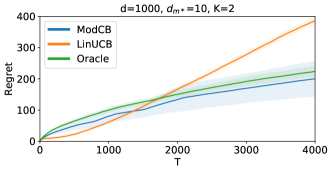
Figure 1: A validation experiment

We consider a simple contextual bandit environment with $K=2$ actions, and where the feature vectors have ambient dimension $d=1000$. We design the reward distribution such that a predictor using the first $d_{m^{\star}}=10$ coordinates is realizable. We consider three algorithms: LinUCB operating directly on the ambient dimension, ModCB with ILTCB as the base learner, and ILTCB with knowledge of $d_{m^{\star}}$, which we refer to as Oracle. We tune a single hyperparameter for each algorithm (the confidence pre-multiplier for LinUCB; the uniform exploration parameter for ModCB and Oracle) and visualize the cumulative regret for the best performing hyperparameter as a function of the number of rounds $T$. Figure 1 displays the regret curves averaged over 20 replicates with error bands corresponding to two standard errors.

ModCB consistently outperforms LinUCB in the experiment, which is unsurprising since the ambient dimension is much larger than the target dimension $d_{m^{\star}}$. ModCB has a less favorable dependence on $T$ in comparison to LinUCB, but this does not seem to compromise its performance in this experiment. Perhaps more surprising is that ModCB outperforms Oracle on average. A deeper inspection reveals that while ModCB typically advances to $d_{m}>d_{m^{\star}}$, it sometimes stays below, where it can learn a near-optimal policy faster than Oracle.

5 Discussion

This paper initiates the study of model selection tradeoffs in contextual bandits. We provide the first model selection algorithm for the linear contextual bandit setting, which we show achieves $\tilde{O}\left(T^{2/3}d_{m^{\star}}^{1/3}\right)$ when the optimal model is a $d_{m^{\star}}$-dimensional linear function. This is the first contextual bandit algorithm that adapts the complexity of the optimal policy class with no prior knowledge, and raises a number of intriguing questions:

1. Is it possible to achieve $\tilde{O}\left(\sqrt{Td_{m^{\star}}}\right)$ regret in our setup? This would show that the price for model selection is negligible.

2. Is it possible to generalize our results beyond linear classes? Specifically, given regressor classes $\mathcal{F}_{1}\subset\mathcal{F}_{2}\subset\ldots\subset\mathcal{F}_{M}$ and assuming the optimal model $f^{\star}$ belongs to $\mathcal{F}_{m^{\star}}$ for some unknown $m^{\star}$, is there a contextual bandit algorithm that achieve $\tilde{O}\left(T^{\alpha}\cdot\textrm{comp}^{1-\alpha}(\mathcal{F}_{m^{\star}})\right)$ regret for some $\alpha\in[\nicefrac{{1}}{{2}},1)$? More ambitiously, can we achieve $\tilde{O}\left(\sqrt{T\cdot\textrm{comp}(\mathcal{F}_{m^{\star}})}\right)$?

3. While this synthetic experiment is encouraging, ModCB may not be immediately useful for practical deployments for several reasons, including its reliance on linear realizability and its computational complexity. Are there more robust algorithmic principles for theoretically-sound and practically-effective model selection in contextual bandits?

4. For what classes $\mathcal{F}$ can we estimate the loss at a sublinear rate, and is this necessary for contextual bandit model selection? Any sublinear guarantee will lead to non-trivial model selection guarantees through a strategy similar to ModCB. Interestingly, it is already known that for certain (e.g., sparse linear) classes, sublinear loss estimation is not possible (Verzelen and Gassiat, 2018). On the other hand, positive results are available for certain nonparametric classes (Brown et al., 2007; Wang et al., 2008).

Model selection is instrumental to the success of ML deployments, yet few positive results exist for partial feedback settings. We believe these questions are technically challenging and practically important, and we are hopeful that positive results of the type we provide here will extend to interactive learning settings beyond contextual bandits.

Acknowledgements

We thank Ruihao Zhu for working with us at the early stages of this project, and for many helpful discussions. AK is supported in part by NSF Award IIS-1763618. HL is supported by NSF IIS-1755781.

Appendix A Omitted details for Section 2

In this section we provide more detail as to why various natural approaches do not provide a satisfactory resolution to the model selection problem for contextual bandits. We consider a more general setup here, where the learner is given a set of policy classes $\Pi_{1},\ldots,\Pi_{M}$, each of which contains a set of arbitrary mappings from the context space $\mathcal{X}$ to $\mathcal{A}$. The (expected) regret to class $m$ is

$$\mathrm{Reg}(\Pi_{m})\vcentcolon=\sum_{t=1}^{T}\mathbb{E}\left[\ell_{t}(a_{t})\right]-\min_{\pi\in\Pi_{m}}\sum_{t=1}^{T}\mathbb{E}\left[\ell_{t}(\pi(x_{t}))\right].$$

Let $m^{\star}\vcentcolon=\mathop{\mathrm{argmin}}_{m}\min_{\pi\in\Pi_{m}}\sum_{t=1}^{T}\mathbb{E}\left[\ell_{t}(\pi(x_{t}))\right]$ be the index of the class containing the optimal policy. The goal is to achieve $\mathrm{Reg}(\Pi_{m^{\star}})=O\left(T^{\alpha}\cdot\textrm{comp}^{1-\alpha}(\Pi_{m^{\star}})\right)$ for some $\alpha\in[\nicefrac{{1}}{{2}},1)$ without knowing $m^{\star}$ ahead of time (ignoring the dependence on $K$). Our realizable linear setting is clearly a special case of this setup. It is well-known that the model selection guarantee we desire can be achieved in the full-information online learning setting, and below we discuss the difficulties of extending these approaches to the bandit setting, even when $M=2$. For simplicity we consider finite classes, so the complexity of $\Pi_{m}$ is measured by $\log|\Pi_{m}|$.

A.1 Running Hedge with all policy classes

The classical contextual bandit algorithm Exp4 (Auer et al., 2002) is based on the full-information algorithm Hedge (Freund and Schapire, 1997). Fix a policy class $\Pi$. At each time $t$, Exp4 computes a distribution $p_{t}$ over the policies in $\Pi$ using the exponential weight update rule:

$$p_{t}(\pi)\propto p_{0}(\pi)\exp\left(\eta\sum_{\tau<t}\hat{\ell}_{\tau}(\pi(x_{\tau}))\right),$$

where $\eta$ is a learning rate parameter, $p_{0}$ is a prespecified prior distribution over the policies, and $\hat{\ell}_{\tau}$ is the importance-weighted loss estimator, defined as $\hat{\ell}_{\tau}(a)\vcentcolon=\frac{\ell_{\tau}(a)\mathbb{I}\{a_{\tau}=a\}}{\sum_{\pi\in\Pi:\pi(x_{\tau})=a}p_{\tau}(\pi)}$ for all $a$. Exp4 ensures for any $\pi^{\star}\in\Pi$,

$$\sum_{t=1}^{T}\mathbb{E}\left[\ell_{t}(a_{t})\right]-\sum_{t=1}^{T}\mathbb{E}\left[\ell_{t}(\pi^{\star}(x_{t}))\right] \leq\frac{\log\left(\frac{1}{p_{0}(\pi^{\star})}\right)}{\eta}+\eta\mathbb{E}\left[\sum_{t=1}^{T}\sum_{\pi\in\Pi}p_{t}(\pi)\hat{\ell}_{t}(\pi(x_{t}))^{2}\right]$$ (9)

$$\leq\frac{\log\left(\frac{1}{p_{0}(\pi^{\star})}\right)}{\eta}+\eta TK.$$

Now, consider running this algorithm with $\Pi\vcentcolon=\bigcup_{m=1}^{M}\Pi_{m}$. With a uniform prior and the optimal tuning of $\eta$, this leads the following regret bound for all $m$, which is clearly undesirable:

$$\mathrm{Reg}(\Pi_{m})=O\left(\sqrt{TK\log\left(\sum_{m=1}^{M}|\Pi_{m}|\right)}\right).$$

On the other hand, if we set $p_{0}(\pi)\vcentcolon=1/(M|\Pi_{m}|)$, where $m$ is the least index such that $\pi\in\Pi_{m}$, then we have that for each $m$,

$$\mathrm{Reg}(\Pi_{m})\leq\frac{\log\left(M|\Pi_{m}|\right)}{\eta}+\eta TK.$$

With oracle tuning for $\eta$ this would give $\mathrm{Reg}(\Pi_{m^{\star}})=\mathrm{Reg}\leq O(\sqrt{TK\log|\Pi_{m^{\star}}|})$, as desired. The issue, of course, is that tuning requires knowing $m^{\star}$ ahead of time. One can instead simply set $\eta=1/\sqrt{TK}$ and obtain for all $m$,

$$\mathrm{Reg}(\Pi_{m})=O\left(\sqrt{TK}\log\left(M|\Pi_{m}|\right)\right),$$

which is not a satisfactory model selection guarantee. In particular this bound is vacuous when $\log|\Pi_{m^{\star}}|=\Omega(\sqrt{T})$, even though we could have achieved sublinear regret here if $m^{\star}$ were known.

A natural next step would be to apply an individual learning rate $\eta_{m}$ for each class separately, with the hope of achieving for all $m$,

$$\mathrm{Reg}(\Pi_{m})=\frac{\log\left(M|\Pi_{m}|\right)}{\eta_{m}}+\eta_{m}TK,$$

which will then solve the problem by setting $\eta_{m}=\sqrt{\log(|\Pi_{m}|)/(TK)}$. However, we are not aware of any existing approaches that achieve this guarantee. The closest guarantee (achieved by variants of Hedge (Gaillard et al., 2014; Koolen and Van Erven, 2015)) is that for all $m$ and $\pi_{m}\in\Pi_{m}$,

$$\sum_{t=1}^{T}\mathbb{E}\left[\ell_{t}(a_{t})\right]-\sum_{t=1}^{T}\mathbb{E}\left[\ell_{t}(\pi_{m}(x_{t}))\right] \leq\frac{\log\left(M|\Pi_{m}|\right)}{\eta_{m}}+\eta_{m}\mathbb{E}\left[\sum_{t=1}^{T}(\ell_{t}(a_{t})-\hat{\ell}_{t}(\pi_{m}(x_{t})))^{2}\right]$$

$$\leq\frac{\log\left(M|\Pi_{m}|\right)}{\eta_{m}}+2\eta_{m}T+2\eta_{m}\mathbb{E}\left[\sum_{t=1}^{T}\hat{\ell}_{t}(\pi_{m}(x_{t}))^{2}\right].$$

Unfortunately, this does not enjoy the useful local norm term as in (9), and in particular the last term involving the second moment of the loss estimator can be unbounded. Common fixes such as forcing a small amount of uniform exploration all lead to further tuning issues.

A.2 Aggregating via Corral

Next, we briefly describe issues with using Corral (Agarwal et al., 2017b) to aggregate multiple instances of Exp4. In short, using Theorem 4 of (Agarwal et al., 2017b), one can verify that the algorithm ensures for all $m$,

$$\mathrm{Reg}(\Pi_{m})=\tilde{O}\left(\frac{M}{\eta}+T\eta-\frac{\rho_{m}}{\eta}+\sqrt{TK\log(|\Pi_{m}|)\rho_{m}}\right),$$

for a fixed parameter $\eta$ and a certain data-dependent quantity $\rho_{m}$. Using the AM-GM inequality to upper bound the last term by $\eta TK\log(|\Pi_{m}|)+\rho_{m}/\eta$, and canceling with the third term, we have $\mathrm{Reg}(\Pi_{m})=\tilde{O}\left(\frac{M}{\eta}+\eta TK\log(|\Pi_{m}|)\right)$. At this point, one can see that the tuning issues similar to those discussed in the previous section appear, and again there is no obvious fix.

A.3 Adaptive $\epsilon$-greedy

Here we present a natural adaptation of an $\epsilon$-greedy algorithm for model selection with two classes $|\Pi_{1}|\ll|\Pi_{2}|$. The algorithm does not achieve a satisfactory model selection guarantee, but we include the analysis because it demonstrates some of the difficulties with parameter tuning, even for algorithms based on naive exploration where the best rate one could hope to achieve is $O(T^{2/3}\mathrm{comp}(\mathcal{F}_{m^{\star}})^{1/3})$.

  Inputs: $T$, policy classes $\Pi_{1},\Pi_{2}$ with $|\Pi_{1}|\leq|\Pi_{2}|$.

  Set $t_{1}\vcentcolon=\lceil T^{2/3}(K\log|\Pi_{1}|)^{1/3}\rceil$, $t_{2}\vcentcolon=\lceil T^{2/3}(K\log|\Pi_{2}|)^{1/3}\rceil$.

  Set $\Delta\vcentcolon=\Omega\left(\left(\frac{K}{T\log(T|\Pi_{1})}\right)^{1/3}\sqrt{\log(T|\Pi_{2}|)}\right)$.

  for $t=1,\ldots,t_{1}$ do

     Observe $x_{t}$ choose $a_{t}\sim\textrm{Unif}(\mathcal{A})$, observe $\ell_{t}(a_{t})$.

  Define $\hat{L}_{1}:\pi\mapsto\sum_{t=1}^{t_{1}}\ell_{t}(a_{t}){\bf 1}\{\pi(x_{t})=a_{t}\}$. Set

$$\hat{\pi}_{1}\vcentcolon=\mathop{\mathrm{argmin}}_{\pi\in\Pi_{1}}\hat{L}_{1}(\pi),\qquad\hat{\pi}_{2}\vcentcolon=\mathop{\mathrm{argmin}}_{\pi\in\Pi_{2}}\hat{L}_{1}(\pi)$$

  if $\hat{L}_{1}(\hat{\pi}_{1})\leq\hat{L}_{1}(\hat{\pi}_{2})+\Delta$ then

     Use $\hat{\pi}_{1}$ to select actions for the rest of time.

  else

     Explore uniformly for a total of $t_{2}$ rounds, let $\hat{\pi}^{(2)}_{2}\vcentcolon=\mathop{\mathrm{argmin}}_{\pi\in\Pi_{2}}\sum_{t=1}^{t_{2}}\ell_{t}(a_{t}){\bf 1}\{\pi(x_{t})=a_{t}\}$, and use $\hat{\pi}_{2}^{(2)}$ to select actions for the rest of time.

Algorithm 3 An adaptive explore-first algorithm.

Pseudocode is displayed in Algorithm 3. The algorithm operates in the stochastic setting, where we have $(x_{t},\ell_{t})\sim\mathcal{D}$ on each round for some distribution $\mathcal{D}$. Define $L(\pi)\vcentcolon=\mathbb{E}_{(x,\ell)\sim\mathcal{D}}\left[\ell(\pi(x))\right]$, and let $\pi_{i}^{\star}\vcentcolon=\mathop{\mathrm{argmin}}_{\pi\in\Pi_{i}}L(\pi)$. We assume that losses are bounded in $[0,1]$.

The algorithm consists of an exploration phase, a statistical test, a second exploration phase depending on the outcome of the test, and then an exploitation phase. The intuition is that we first explore for $t_{1}$ rounds, where $t_{1}$ is the optimal hyperparameter choice for the smaller class $\Pi_{1}$ (smaller classes require less exploration). Then, we perform a statistical test to determine if $\Pi_{1}$ can achieve loss that is competitive with $\Pi_{2}$. If this is the case, we simply exploit $\Pi_{1}$ for the remaining rounds. Otherwise, we continue exploring for a total of $t_{2}$ rounds, where $t_{2}$ is the optimal hyperparameter for $\Pi_{2}$. We finish by exploiting with the empirical risk minimizer for $\Pi_{2}$.

Proposition 6.

In the stochastic setting, Algorithm 3 achieves the following guarantees simultaneously with probability at least $1-1/T$:

$$\mathrm{Reg}(\Pi_{1})\leq\tilde{O}\left(T^{2/3}(K\log|\Pi_{1}|)^{1/3}\right),\quad\text{and}\quad\mathrm{Reg}(\Pi_{2})\leq\tilde{O}\left(T^{2/3}K^{1/3}\frac{\log^{1/2}|\Pi_{2}|}{\log^{1/3}|\Pi_{1}|}\right).$$

Note that this is not a satisfactory model selection guarantee, since the exponents on $T$ and the policy complexity for $\Pi_{2}$ do not sum to $1$ as we would like. Conceptually, if the algorithm exploits with a fixed policy, it must first determine whether $\Pi_{2}$ offers much lower loss than $\Pi_{1}$ so that it can decide which class to use for exploitation. To make this determination, it must estimate the optimal loss for both classes. Unfortunately, with too little exploration data, we will significantly underestimate the loss for $\Pi_{2}$, and with too much data we will compromise the regret bound for $\Pi_{1}$. We are not aware of an approach to balance these competing objectives with this style of algorithm.

Proof of Proposition 6.

Define $\hat{L}_{2}:\pi\mapsto\sum_{t=1}^{t_{2}}\ell_{t}(a_{t}){\bf 1}\{\pi(x_{t})=a_{t}\}$. We will only use $\hat{L}_{2}$ in the event that we continue to explore after the test. Via Bernstein’s inequality (and using that the deviation is at most $1$), the following inequalities all hold with probability at least $1-\delta$:

$$\forall j\in[2],\forall\pi\in\Pi_{i}:\left|L(\pi)-\hat{L}_{j}(\pi)\right| \leq c\sqrt{\frac{K\log(|\Pi_{i}|/\delta)}{t_{j}}},$$

$$\forall i\in[2]:\left|L(\pi_{i}^{\star})-\hat{L}_{1}(\pi_{i}^{\star})\right| \leq c\sqrt{\frac{K\log(1/\delta)}{t_{1}}}.$$

Note that the second inequality does not use uniform convergence, and it applies only to each $\pi_{i}^{\star}$. Appealing to the standard explore-first analysis, we know that the regret bound for $\Pi_{1}$ is achieved if we exploit with $\hat{\pi}_{1}$, and similarly for $\Pi_{2}$ if we exploit with $\hat{\pi}_{2}^{(2)}$. We are left to verify the other two cases. Let us consider $\mathrm{Reg}(\Pi_{2})$ when we only explore for $t_{1}$ rounds. We have

$$\mathrm{Reg}(\Pi_{2}) =t_{1}+(T-t_{1})\left(L(\hat{\pi}_{1})-L(\pi_{2}^{\star})\right)$$

$$\leq t_{1}+T\left(c\sqrt{\frac{K\log(|\Pi_{1}|/\delta)}{t_{1}}}+\Delta+c\sqrt{\frac{K\log(1/\delta)}{t_{1}}}\right)$$

$$\leq t_{1}+2c\sqrt{\frac{KT\log(|\Pi_{1}|/\delta)}{t_{1}}}+T\Delta.$$

Here we use the two concentration inequalities above, the fact that $\hat{L}_{1}(\pi_{2}^{\star})\geq\hat{L}_{1}(\hat{\pi}_{2})$, and the fact that the test succeeded. Note that we did not require uniform convergence over $\Pi_{2}$ for this argument. Now, let us consider the regret for $\Pi_{1}$ when we explore for $t_{2}$ rounds.

$$\mathrm{Reg}(\Pi_{1})$$

$$=t_{2}+(T-t_{2})\left(L(\hat{\pi}_{2}^{(2)})-L(\pi_{1}^{\star})\right)$$

$$\leq t_{2}+(T-t_{2})\left(c\sqrt{\frac{K\log(|\Pi_{2}|/\delta)}{t_{2}}}+L(\pi_{2}^{\star})-\hat{L}_{1}(\hat{\pi}_{1})+c\sqrt{\frac{K\log(1/\delta)}{t_{1}}}\right)$$

$$\leq t_{2}+(T-t_{2})\left(c\sqrt{\frac{K\log(|\Pi_{2}|/\delta)}{t_{2}}}+c\sqrt{\frac{K\log(|\Pi_{2}|/\delta)}{t_{1}}}+\hat{L}_{1}(\hat{\pi}_{2})-\hat{L}_{1}(\hat{\pi}_{1})+c\sqrt{\frac{K\log(1/\delta)}{t_{1}}}\right)$$

$$\leq 4c(T-t_{2})\sqrt{\frac{K\log(|\Pi_{2}|/\delta)}{t_{1}}}-(T-t_{2})\Delta,$$

where we have used that $t_{2}$ is lower order than the deviation bound term, since $t_{1}$ is much smaller. To obtain the claimed regret bound for $\Pi_{1}$, we must choose $\Delta$ as

$$\Delta\geq 4c\sqrt{\frac{K\log(|\Pi_{2}|/\delta)}{t_{1}}}-\Omega\left((K\log(|\Pi_{1}|/\delta)/T)^{1/3}\right)=\Omega\left(\left(\frac{K}{T\log(|\Pi_{1}|/\delta)}\right)^{1/3}\sqrt{\log(|\Pi_{2}|/\delta)}\right),$$

with $\delta=1/T$. ∎

Appendix B Preliminaries for main results

This section consists of self-contained technical results used to prove the main theorem.

B.1 Properties of subgaussian and subexponential random variables

Here we state some standard facts about subgaussian and subexponential random variables that will be used throughout the analysis. The reader may consult e.g., Vershynin (2012), for proofs.

Note that if $z\sim\mathsf{subG}_{d}(\tau^{2})$ then we clearly have $\left\langle z,\theta\right\rangle\sim\mathsf{subG}(\tau^{2}\left\|\theta\right\|_{2}^{2})$ and likewise if $z\sim\mathsf{subE}_{d}(\lambda)$ then $\left\langle z,\theta\right\rangle\sim\mathsf{subE}(\lambda\left\|\theta\right\|_{2})$. Furthermore, if $z\sim\mathsf{subG}_{d}(\sigma^{2})$, then $\operatorname{\mathbb{E}}\left[zz^{\top}\right]\preceq\sigma^{2}\cdot{}I_{d}$.

Proposition 7.

There exist universal constants $c_{1},c_{2},c_{3}>0$ such that for any random variable $z\sim\mathsf{subG}(\sigma^{2})$, the following hold:

• $\operatorname{Pr}(\left\lvert z\right\rvert>t)\leq{}2e^{-\frac{t^{2}}{c_{1}\sigma^{2}}}\quad\forall{}t\geq{}0$.

• $\operatorname{\mathbb{E}}[\exp(c_{2}\left\lvert z\right\rvert^{2}/\sigma^{2})]\leq{}2$.

• If $\operatorname{\mathbb{E}}\left[z\right]=0$, $\operatorname{\mathbb{E}}\left[\exp\left(sz\right)\right]\leq{}\exp\left(c_{3}s^{2}\sigma^{2}\right)\quad\forall{}s\in\mathbb{R}^{d}$.

Moreover, there is some universal constant $c_{4}$ such that if any of the above properties hold, then $z\sim\mathsf{subG}(c_{4}\sigma^{2})$

Proposition 8.

There exist universal constants $c_{1},c_{2},c_{3}>0$ such that for any random variable $z\sim\mathsf{subE}(\lambda)$, the following hold:

• $\operatorname{Pr}(\left\lvert z\right\rvert>t)\leq{}2e^{-\frac{t}{c_{1}\lambda}}\quad\forall{}t\geq{}0$.

• If $\operatorname{\mathbb{E}}\left[z\right]=0$, $\operatorname{\mathbb{E}}\left[\exp\left(sz\right)\right]\leq{}\exp\left(c_{2}s^{2}\lambda^{2}\right)\quad\forall{}s:\left\lvert s\right\rvert\leq{}\frac{1}{c_{3}\lambda}$.

Moreover, there is some universal constant $c_{4}$ such that if any of the above properties hold, then $z\sim\mathsf{subE}(c_{4}\lambda)$

Proposition 9.

There is a universal constant $c>0$ such that the following hold:

• If $z\sim\mathsf{subG}(\sigma^{2})$, $z-\operatorname{\mathbb{E}}\left[z\right]\sim\mathsf{subG}(4\sigma^{2})$, and if $z\sim\mathsf{subE}(\lambda)$, $z-\operatorname{\mathbb{E}}\left[z\right]\sim\mathsf{subE}(2\lambda)$.

• If $z\sim\mathsf{subG}(\sigma^{2})$, then $z^{2}-\operatorname{\mathbb{E}}\left[z^{2}\right]\sim\mathsf{subE}(c\cdot\sigma^{2})$.

• If $z_{1}\sim\mathsf{subG}(\sigma^{2}_{1})$ and $z_{2}\sim\mathsf{subG}(\sigma_{2}^{2})$, then $z_{1}z_{2}-\operatorname{\mathbb{E}}\left[z_{1}z_{2}\right]\sim{}\mathsf{subE}(c\cdot\sigma_{1}\sigma_{2})$.

Proposition 10 (Bernstein’s inequality for subexponential random variables).

Let $z_{1},\ldots,z_{n}$ be independent mean-zero random variables with $z_{i}\sim\mathsf{subE}(\lambda)$ for all $i$, and let $Z=\sum_{i=1}^{n}z_{i}$. Then for some universal constant $c>0$,

$$\operatorname{Pr}\left(\left\lvert Z\right\rvert\geq{}t\right)\leq{}2\exp\left(-c\left(\frac{t^{2}}{\lambda^{2}n}\wedge\frac{t}{\lambda}\right)\right).$$

In particular, with probability at least $1-\delta$, $\left\lvert Z\right\rvert\leq{}O\left(\sqrt{n\lambda^{2}\log(2/\delta)}+\lambda\log(2/\delta)\right)$.

Lemma 11.

Let $z_{1},\ldots{}z_{n}$ be i.i.d. draws of a mean-zero random variable $z\sim\mathsf{subE}_{d}(\lambda)$, and let $Z_{i}=\sum_{t=1}^{i}z_{t}$. Then with probability at least $1-\delta$,

$$\max_{i\in\left[n\right]}\left\|Z_{i}\right\|_{2}\leq{}O\left(\lambda\sqrt{dn\log(2d/\delta)}+\lambda{}d^{1/2}\log(2d/\delta)\right).$$

Proof of Lemma 11.

We first claim that for any $s>0$, the sequence $X_{i}\vcentcolon={}e^{s\left\|Z_{i}\right\|_{2}}$ is a non-negative submartingale. Indeed, using Jensen’s inequality, we have

$$\operatorname{\mathbb{E}}\left[X_{i}\mid{}z_{1},\ldots,z_{i-1}\right]=\operatorname{\mathbb{E}}\left[e^{s\left\|\sum_{t=1}^{i}z_{t}\right\|_{2}}\mid{}z_{1},\ldots,z_{i-1}\right]\geq{}\operatorname{\mathbb{E}}\left[e^{s\left\|\sum_{t=1}^{i-1}z_{t}\right\|_{2}}\mid{}z_{1},\ldots,z_{i-1}\right]=X_{i-1}.$$

Thus, applying the Chernoff method along with Doob’s maximal inequality, we have

$$\operatorname{Pr}\left(\max_{i\in\left[n\right]}\left\|Z_{i}\right\|_{2}>t\right)\leq{}\operatorname{\mathbb{E}}\left[\exp\left(s\left\|\sum_{t=1}^{n}z_{t}\right\|_{2}-st\right)\right].$$

We apply the bound

$$\operatorname{\mathbb{E}}\left[\exp\left(s\left\|\sum_{t=1}^{n}z_{t}\right\|_{2}\right)\right]\leq{}\operatorname{\mathbb{E}}\left[\exp\left(s\sqrt{d}\left\|\sum_{t=1}^{n}z_{t}\right\|_{\infty}\right)\right]\leq{}\sum_{k=1}^{d}\operatorname{\mathbb{E}}\left[\exp\left(s\sqrt{d}\left\lvert\left\langle\sum_{t=1}^{n}z_{t},e_{k}\right\rangle\right\rvert\right)\right],$$

where $e_{k}$ is the $k$th standard basis vector. Since $z_{t}\sim\mathsf{subE}_{d}(\lambda)$ and $\left\{z_{t}\right\}$ are independent, the latter quantity is bounded by

$$2d\cdot\exp\left(Cs^{2}d\lambda^{2}n\right),$$

so long as $s\leq{}1/c\lambda{}\sqrt{d}$, for absolute constants $C,c>0$. We set $s\propto\frac{t}{d\lambda^{2}n}\wedge\frac{1}{\lambda{}\sqrt{d}}$ to conclude

$$\operatorname{Pr}\left(\max_{i\in\left[n\right]}\left\|Z_{i}\right\|_{2}>t\right)\leq{}2d\cdot{}e^{-C\left(\frac{t^{2}}{d\lambda^{2}n}\vee\frac{t}{\lambda{}\sqrt{d}}\right)}.$$

Or in other words, with probability at least $1-\delta$,

$$\max_{i\in\left[n\right]}\left\|Z_{i}\right\|_{2}\leq{}O\left(\lambda\sqrt{dn\log(2d/\delta)}+\lambda{}d^{1/2}\log(2d/\delta)\right).$$ ∎

B.2 Second moment matrix estimation

In this section we give some standard results for the rate at which the empirical correlation matrix approaches the population correlation matrix for subgaussian random variables. Let $x\sim\mathsf{subG}_{d}(\tau^{2})$ be a subgaussian random variable and let $\Sigma=\operatorname{\mathbb{E}}\left[xx^{\top}\right]$. Let $x_{1},\ldots,x_{n}$ be i.i.d. draws from $x$, and let $\widehat{\Sigma}=\frac{1}{n}\sum_{t=1}^{n}x_{t}x_{t}^{\top}$.

Proposition 12.

Suppose $x\sim{}\mathsf{subG}_{d}(\tau^{2})$ and $\Sigma=I$. Then with probability at least $1-\delta$,

$$1-\varepsilon\leq{}\lambda_{\mathrm{min}}^{1/2}(\widehat{\Sigma})\leq{}\lambda_{\mathrm{max}}^{1/2}(\widehat{\Sigma})\leq{}1+\varepsilon,$$ (10)

where $\varepsilon\leq{}50\tau^{2}\sqrt{\frac{d+\log(2/\delta)}{n}}$.

Proof of Proposition 12.

Tracking constants carefully, equation (5.23) in Vershynin (2012) establishes that with probability at least $1-2e^{-\frac{ct^{2}}{\tau^{4}}}$,

$$\left\|\widehat{\Sigma}-I\right\|_{2}\leq{}\varepsilon\vee\varepsilon^{2},$$

where $\varepsilon=C\tau^{2}\sqrt{\frac{d}{n}}+\frac{t}{\sqrt{n}}$, and $c>10^{-3}$ and $C\leq{}25$ are absolute constants. The result follows by Vershynin (2012), Lemma 5.36. ∎

Proposition 13.

Let $\Sigma$ be positive definite, and suppose $\widehat{\Sigma}$ is such that

$$1-\varepsilon\leq{}\lambda_{\mathrm{min}}^{1/2}(\Sigma^{-1/2}\widehat{\Sigma}\Sigma^{-1/2})\leq{}\lambda_{\mathrm{max}}^{1/2}(\Sigma^{-1/2}\widehat{\Sigma}\Sigma^{-1/2})\leq{}1+\varepsilon,$$

where $\varepsilon\leq{}1/2$. Then the following inequality holds:

$$1-2\varepsilon\leq{}\lambda_{\mathrm{min}}^{1/2}(\Sigma^{1/2}\widehat{\Sigma}^{-1}\Sigma^{1/2})\leq{}\lambda_{\mathrm{max}}^{1/2}(\Sigma^{1/2}\widehat{\Sigma}^{-1}\Sigma^{1/2})\leq{}1+2\varepsilon,$$

and furthermore,

$$\left\|\widehat{\Sigma}-\Sigma\right\|_{2} \leq{}\lambda_{\mathrm{max}}(\Sigma)\cdot{}3\varepsilon,$$ (11)

$$\left\|\widehat{\Sigma}^{-1}-\Sigma^{-1}\right\|_{2} \leq{}\frac{6\varepsilon}{\lambda_{\mathrm{min}}(\Sigma)},$$ (12)

$$\left\|\Sigma^{-1/2}\widehat{\Sigma}\Sigma^{-1/2}-I\right\|_{2} \leq{}3\varepsilon,$$ (13)

$$\left\|\Sigma^{1/2}\widehat{\Sigma}^{-1}\Sigma^{1/2}-I\right\|_{2} \leq{}6\varepsilon.$$ (14)

Proof of Proposition 13.

To begin, note that the assumed inequality immediately implies that $\widehat{\Sigma}^{-1}$ is well-defined and that

$$1-2\varepsilon\leq{}\lambda_{\mathrm{min}}^{1/2}(\Sigma^{1/2}\widehat{\Sigma}^{-1}\Sigma^{1/2})\leq{}\lambda_{\mathrm{max}}^{1/2}(\Sigma^{1/2}\widehat{\Sigma}^{-1}\Sigma^{1/2})\leq{}1+2\varepsilon,$$

using the elementary fact that $(1-\varepsilon)^{-1}\leq{}1+2\varepsilon$ and $(1+\varepsilon)^{-1}\geq{}1-2\varepsilon$ when $\varepsilon\leq{}1/2$. This inequality and the assumed inequality, together with Lemma 5.36 of Vershynin (2012) imply that

$$\left\|\Sigma^{-1/2}\widehat{\Sigma}\Sigma^{-1/2}-I\right\|_{2}\leq{}3\varepsilon,\quad\text{and}\quad\left\|\Sigma^{1/2}\widehat{\Sigma}^{-1}\Sigma^{1/2}-I\right\|_{2}\leq{}6\varepsilon.$$

Finally, observe that we can write

$$\left\|\widehat{\Sigma}-\Sigma\right\|_{2}=\left\|\Sigma^{1/2}(\Sigma^{-1/2}\widehat{\Sigma}\Sigma^{-1/2}-I)\Sigma^{1/2}\right\|_{2}\leq{}\lambda_{\mathrm{max}}(\Sigma)\cdot\left\|\Sigma^{-1/2}\widehat{\Sigma}\Sigma^{-1/2}-I\right\|_{2},$$

and

$$\left\|\widehat{\Sigma}^{-1}-\Sigma^{-1}\right\|_{2}=\left\|\Sigma^{-1/2}(\Sigma^{1/2}\widehat{\Sigma}^{-1}\Sigma^{1/2}-I)\Sigma^{-1/2}\right\|_{2}\leq{}\frac{1}{\lambda_{\mathrm{min}}(\Sigma)}\cdot\left\|\Sigma^{1/2}\widehat{\Sigma}^{-1}\Sigma^{1/2}-I\right\|_{2}.$$

This establishes the result. ∎

B.3 Agnostic contextual bandit algorithm for Natarajan classes (Exp4-IX)

  Input: policy class $\Pi$ with Natarajan dimension $d$, maximum number of rounds $T$, confidence parameter $\delta$.

  for $k=0,1,\ldots$ do

     Explore uniformly at random for $n_{k}=\sqrt{2^{k}d\log\left(\frac{TK}{\delta}\right)}$ rounds.

     $t\leftarrow{}2^{k}+n_{k}$, $\eta_{k}\leftarrow{}\sqrt{\frac{d\log\left(\frac{TK}{\delta}\right)}{2^{k}K}}$.

     Let $\Pi_{k}\in\Pi$ be the set of unique policies witnessed by $x_{2^{k}},\ldots,x_{t-1}$ (choose a representative from each equivalence class).

     Initialize $P_{t}$ to be the uniform distribution over $\Pi_{k}$.

     while $t<2^{k+1}$ do

        Receive $x_{t}$, sample an action $a_{t}\sim P_{t}(\cdot|x_{t})$, and observe $\ell_{t}(a_{t})$.

        Compute $P_{t+1}$ such that $P_{t+1}(\pi)\propto P_{t}(\pi)\exp\left(\frac{-2\eta_{k}\left(\frac{\ell_{t}(a_{t})}{b}+1\right){\bf 1}\left\{a_{t}=\pi(x_{t})\right\}}{P_{t}(a_{t}|x_{t})+\eta_{k}}\right),~{}\forall\pi\in\Pi_{k}$.

        $t\leftarrow{}t+1$.

Algorithm 4 Exp4-IX with Natarajan class and anytime guarantee

Here we present a variant of the Exp4-IX algorithm (Neu, 2015), originally proposed for achieving high-probability regret bounds for contextual bandits with a finite policy class and bounded non-negative losses. There are three main differences in the variant we present here (see Algorithm 4 for the pseudocode).

First, for our application we need an “anytime” regret guarantee that holds for any time $T^{\prime}\leq T$. This can be simply achieved by a standard doubling trick. Specifically, we run the algorithm on an exponential epoch schedule (that is, epoch $k$ lasts for $2^{k}$ rounds) and restart Exp4-IX at the beginning of each epoch with new parameters.

Second, our policy class is infinite, but with a finite Natarajan dimension. For the two-action case with a VC class, Beygelzimer et al. (2011) gave a solution to this problem for stochastic contextual bandits. We extend their approach to Natarajan classes. Specifically, in epoch $k$ we spend the first $n_{k}$ rounds collecting contexts (while picking actions arbitrarily). Then we form a finite policy subset $\Pi_{k}$ by picking one representative from each equivalence class (that is, all policies that behave exactly the same on these contexts), and play Exp4-IX using this finite policy class $\Pi_{k}$ for the rest of the epoch.

Finally, in our setting losses are subgaussian and potentially unbounded. However, since with high probability they are bounded essentially by the subgaussian parameter (see Proposition 19), we simply pick $b=O\left(\tau\log^{1/2}\left(\frac{TK}{\delta}\right)\right)$ such that with probability at least $1-\delta/3$, $\max_{a\in\mathcal{A},t\in\left[T\right]}\left\lvert\ell_{t}(a)\right\rvert\leq{}b$, and transform every loss $\ell(a)$ as $\ell(a)/b+1$, which with high probability falls in $[0,2]$. The rest of the algorithm is the same as the original Exp4-IX. Note that we use the notation $P_{t}(a|x_{t})$ to denote $\sum_{\pi:\pi(x_{t})=a}P_{t}(\pi)$.

The regret guarantee for Algorithm 4 is as follows.

Proposition 14.

With probability at least $1-\delta$, Algorithm 4 ensures that for all $T^{\prime}\in\left\{1,\ldots,T\right\}$ and $\pi\in\Pi$,

$$\sum_{t=1}^{T^{\prime}}\ell_{t}(a_{t})-\ell_{t}(\pi(x_{t}))=O\left(\tau\sqrt{T^{\prime}Kd}\log\left(\frac{TK}{\delta}\right)\right)$$

Proof of Proposition 14.

We condition on the event $\max_{a\in\mathcal{A},t\in\left[T\right]}\left\lvert\ell_{t}(a)\right\rvert\leq{}b$ which happens with probability at least $1-\delta/3$. Following (Neu, 2015), with probability at least $1-\delta/3$ we have for any $T^{\prime}$ and any $\pi\in\Pi_{k}$ (where $k$ is the epoch containing $T^{\prime}$),

$$\sum_{t=2^{k}}^{T^{\prime}}\ell_{t}(a_{t})-\ell_{t}(\pi(x_{t}))=O\left(bn_{k}+b\sqrt{2^{k}K\left(\log|\Pi_{k}|+\log\left(\frac{TK}{\delta}\right)\right)}\right).$$

Sauer’s lemma for classes with finite Natarajan dimension (Ben-David et al., 1995; Haussler and Long, 1995) gives $\log|\Pi_{k}|\leq d\log\left(\frac{n_{k}e(K+1)^{2}}{2d}\right)$. Together with the choice of $n_{k}$ this gives

$$\sum_{t=2^{k}}^{T^{\prime}}\ell_{t}(a_{t})-\ell_{t}(\pi(x_{t}))=O\left(b\sqrt{2^{k}Kd\log\left(\frac{TK}{\delta}\right)}\right).$$

On the other hand, following Beygelzimer et al. (2011) we have with probability at least $1-\delta/3$,

$$\min_{\pi\in\Pi_{k}}\sum_{t=2^{k}}^{T^{\prime}}\ell_{t}(\pi(x_{t})) \leq\min_{\pi\in\Pi}\sum_{t=2^{k}}^{T^{\prime}}\ell_{t}(\pi(x_{t}))+O\left(\frac{b2^{k}d}{n_{k}}\log\left(\frac{TK}{\delta}\right)\right)$$

$$\leq\min_{\pi\in\Pi}\sum_{t=2^{k}}^{T^{\prime}}\ell_{t}(\pi(x_{t}))+O\left(b\sqrt{2^{k}d\log\left(\frac{TK}{\delta}\right)}\right).$$

Combining these inequalities gives

$$\sum_{t=2^{k}}^{T^{\prime}}\ell_{t}(a_{t})\leq\min_{\pi\in\Pi}\sum_{t=2^{k}}^{T^{\prime}}\ell_{t}(\pi(x_{t}))+O\left(b\sqrt{2^{k}Kd\log\left(\frac{TK}{\delta}\right)}\right).$$

Summing up regret in each epoch, using $b=O\left(\tau\log^{1/2}\left(\frac{TK}{\delta}\right)\right)$, and applying a union bound leads to the result. ∎

B.4 Natarajan dimension for linear policy classes

Proposition 15 (Daniely et al. (2015)).

Let $\phi(x,a)\in\mathbb{R}^{d}$ be a fixed feature map and consider the policy class

$$\Pi=\left\{x\mapsto{}\mathop{\mathrm{argmax}}_{a\in\left[K\right]}\left\langle\beta,\phi(x,a)\right\rangle\mid{}\beta\in\mathbb{R}^{d}\right\}.$$

The Natarajan dimension of $\Pi$ is at most $O(d\log{}d)$.

Appendix C Proofs from Section 3

C.1 Square loss residual estimation

In this section we give self-contained results on estimating the square loss in a linear regression setup, extending the results of Dicker (2014) and Kong and Valiant (2018). Our main result here is the sample complexity bound for EstimateResidual described in Section 3

We first recall the abstract setting. We receive pairs $(x_{1},y_{1}),\ldots,(x_{n},y_{n})$ i.i.d. from a distribution $\mathcal{D}\in\Delta(\mathbb{R}^{d}\times{}\mathbb{R})$, where $x\sim\mathsf{subG}_{d}(\tau^{2})$ and $y\sim\mathsf{subG}(\sigma^{2})$. Define $\Sigma\vcentcolon=\operatorname{\mathbb{E}}\left[xx^{\top}\right]$, and assume $\Sigma\succ{}0$. Let $\beta^{\star}\in\mathbb{R}^{d}$ be the predictor that minimizes prediction error:

$$\beta^{\star}\vcentcolon=\mathop{\mathrm{argmin}}_{\beta\in\mathbb{R}^{d}}\operatorname{\mathbb{E}}\left(\left\langle\beta,x\right\rangle-y\right)^{2}.$$

Suppose $x$ can be partitioned into features $x=(x^{(1)},x^{(2)})$, where $x^{(1)}\in\mathbb{R}^{d_{1}}$ and $x^{(2)}\in\mathbb{R}^{d_{2}}$, and $d_{1}+d_{2}=d$. We define $\beta^{\star}_{1}$ to be the optimal predictor when we regress only onto the features $x^{(1)}$:

$$\beta^{\star}_{1}\vcentcolon=\mathop{\mathrm{argmin}}_{\beta\in\mathbb{R}^{d_{1}}}\operatorname{\mathbb{E}}\left(\langle\beta,x^{(1)}\rangle-y\right)^{2}.$$

Our goal is to estimate the residual error incurred by restricting to the features $x^{(1)}$:

$$\mathcal{E}\vcentcolon=\operatorname{\mathbb{E}}\left(\langle\beta^{\star}_{1},x^{(1)}\rangle-\left\langle\beta^{\star},x\right\rangle\right)^{2}.$$

EstimateResidual (Algorithm 2) estimates $\mathcal{E}$ with sample complexity sublinear in $d$ whenever good estimates for the matrices $\Sigma$ and $\Sigma_{1}\vcentcolon=\operatorname{\mathbb{E}}\left[x^{(1)}x^{(1)\top}\right]$ are available. The performance is stated in Theorem 16. The result here is a more general version of Theorem 2, which is proven as a corollary at the end of the section.

Theorem 16.

Suppose the correlation matrix estimates $\widehat{\Sigma}$ and $\widehat{\Sigma}_{1}$ are such that

$$1-\varepsilon\leq{}\lambda_{\mathrm{min}}^{1/2}(\Sigma^{-1/2}\widehat{\Sigma}\Sigma^{-1/2})\leq{}\lambda_{\mathrm{max}}^{1/2}(\Sigma^{-1/2}\widehat{\Sigma}\Sigma^{-1/2})\leq{}1+\varepsilon,$$

and

$$1-\varepsilon\leq{}\lambda_{\mathrm{min}}^{1/2}(\Sigma_{1}^{-1/2}\widehat{\Sigma}_{1}\Sigma^{-1/2}_{1})\leq{}\lambda_{\mathrm{max}}^{1/2}(\Sigma^{-1/2}_{1}\widehat{\Sigma}_{1}\Sigma^{-1/2}_{1})\leq{}1+\varepsilon,$$

where $\varepsilon\leq{}1/2$. Then EstimateResidual guarantees that with probability at least $1-\delta$,

$$\left\lvert\widehat{\mathcal{E}}-\mathcal{E}\right\rvert\leq{}\frac{1}{2}\mathcal{E}+O\left(\frac{\lambda_{\mathrm{max}}(\Sigma)}{\lambda_{\mathrm{min}}^{2}(\Sigma)}\cdot\frac{\sigma^{2}\tau^{2}d^{1/2}\log^{2}(2d/\delta)}{n}+\frac{\lambda_{\mathrm{max}}(\Sigma)}{\lambda_{\mathrm{min}}^{2}(\Sigma)}\left\|\operatorname{\mathbb{E}}\left[xy\right]\right\|_{2}^{2}\cdot\varepsilon^{2}\right).$$ (15)

Proof of Theorem 16.

We begin by giving an expression for $\mathcal{E}$ that will make the choice of estimator more transparent. Let

$$D=\left(\begin{array}[]{ll}\Sigma_{1}&0_{d_{1}\times{}d_{2}}\\ 0_{d_{2}\times{}d_{1}}&0_{d_{2}\times{}d_{2}}\end{array}\right),$$

and let $R=D^{\dagger}-\Sigma^{-1}$. Observe that by first-order conditions, we may take $\beta^{\star}=\Sigma^{-1}\operatorname{\mathbb{E}}\left[xy\right]$ and $\beta^{\star}_{1}=\Sigma_{1}^{-1}\operatorname{\mathbb{E}}\left[x^{(1)}y\right]$. Moreover, for any $x$, we may write $\left\langle\beta^{\star}_{1},x^{(1)}\right\rangle=\left\langle D^{\dagger}\operatorname{\mathbb{E}}\left[xy\right],x\right\rangle$. Consequently, we have

$$\mathcal{E} =\operatorname{\mathbb{E}}\left(\langle D^{\dagger}\operatorname{\mathbb{E}}\left[xy\right],x\rangle-\left\langle\Sigma^{-1}\operatorname{\mathbb{E}}\left[xy\right],x\right\rangle\right)^{2}=\operatorname{\mathbb{E}}\langle R\operatorname{\mathbb{E}}\left[xy\right],x\rangle^{2}=\left\|\Sigma^{1/2}R\operatorname{\mathbb{E}}\left[xy\right]\right\|_{2}^{2}.$$

With this representation, it is clear that if $\widehat{\Sigma}=\Sigma$ and $\widehat{\Sigma}_{1}=\Sigma_{1}$, then $\widehat{\mathcal{E}}$ is an unbiased estimator for $\mathcal{E}$. Our proof has two parts: We first show that $\widehat{\mathcal{E}}$ concentrates around its expectation, then bound the bias due to $\widehat{\Sigma}$ and $\widehat{\Sigma}_{1}$.

For concentration, we appeal to Lemma 17. Note that $\lambda_{\mathrm{min}}(\Sigma_{1})\geq{}\lambda_{\mathrm{min}}(\Sigma)$ and $\lambda_{\mathrm{max}}(\Sigma_{1})\leq{}\lambda_{\mathrm{max}}(\Sigma)$; this can be seen using the variational representation for the eigenvalues. Consequently by Proposition 13 we have that

$$\lambda_{\mathrm{max}}(\widehat{\Sigma})\vee\lambda_{\mathrm{max}}(\widehat{\Sigma}_{1}) \leq{}O(\lambda_{\mathrm{max}}(\Sigma)),\quad\text{and},\quad\lambda_{\mathrm{min}}(\widehat{\Sigma})\wedge\lambda_{\mathrm{min}}(\widehat{\Sigma}_{1})\geq{}\Omega\left(\lambda_{\mathrm{min}}(\Sigma)\right).$$

This implies that

$$\left\|\widehat{\Sigma}^{1/2}\widehat{R}\right\|_{2}\leq{}O\left(\lambda_{\mathrm{max}}^{1/2}(\Sigma)/\lambda_{\mathrm{min}}(\Sigma)\right),$$

and so by Proposition 9, it follows that the random variable $\widehat{\Sigma}^{1/2}\widehat{R}xy-\operatorname{\mathbb{E}}\left[\widehat{\Sigma}^{1/2}\widehat{R}xy\right]$ has subexponential parameter of order $O(\sigma\tau\lambda_{\mathrm{max}}^{1/2}(\Sigma)/\lambda_{\mathrm{min}}(\Sigma))$. Thus, by Lemma 17, we have that with probability at least $1-\delta$,

$$\left\lvert\widehat{\mathcal{E}}-\operatorname{\mathbb{E}}\left[\widehat{\mathcal{E}}\right]\right\rvert\leq{}O\left(\frac{\lambda_{\mathrm{max}}(\Sigma)}{\lambda_{\mathrm{min}}^{2}(\Sigma)}\frac{\sigma^{2}\tau^{2}d^{1/2}\log^{2}(2d/\delta)}{n}+\frac{\lambda_{\mathrm{max}}^{1/2}(\Sigma)}{\lambda_{\mathrm{min}}(\Sigma)}\frac{\sigma\tau\left\|\widehat{\Sigma}^{1/2}\widehat{R}\operatorname{\mathbb{E}}\left[xy\right]\right\|_{2}\log(2/\delta)}{\sqrt{n}}\right).$$

But note that since $\left\|\widehat{\Sigma}^{1/2}\widehat{R}\operatorname{\mathbb{E}}\left[xy\right]\right\|_{2}=\sqrt{\operatorname{\mathbb{E}}\left[\widehat{\mathcal{E}}\right]}$, we can apply the AM-GM inequality to deduce

$$\left\lvert\widehat{\mathcal{E}}-\operatorname{\mathbb{E}}\left[\widehat{\mathcal{E}}\right]\right\rvert\leq{}\frac{1}{8}\operatorname{\mathbb{E}}\left[\widehat{\mathcal{E}}\right]+O\left(\frac{\lambda_{\mathrm{max}}(\Sigma)}{\lambda_{\mathrm{min}}^{2}(\Sigma)}\cdot\frac{\sigma^{2}\tau^{2}d^{1/2}\log^{2}(2d/\delta)}{n}\right).$$

We now bound the error from $\operatorname{\mathbb{E}}\left[\widehat{\mathcal{E}}\right]$ to $\mathcal{E}$. With the shorthand $\mu=\operatorname{\mathbb{E}}\left[xy\right]$, observe that we have

$$\operatorname{\mathbb{E}}\left[\widehat{\mathcal{E}}\right]-\mathcal{E} =\left\langle\widehat{R}\widehat{\Sigma}\widehat{R}\mu,\mu\right\rangle-\left\langle R\Sigma{}R\mu,\mu\right\rangle$$

$$=2\left\langle(\widehat{R}-R)\widehat{\Sigma}{}R\mu,\mu\right\rangle+\left\langle R(\widehat{\Sigma}-\Sigma)R\mu,\mu\right\rangle+\left\langle(\widehat{R}-R)\widehat{\Sigma}(\widehat{R}-R)\mu,\mu\right\rangle.$$

Applying Cauchy-Schwarz to each term, we get an upper bound of

$$\left\lvert\operatorname{\mathbb{E}}\left[\widehat{\mathcal{E}}\right]-\mathcal{E}\right\rvert \leq 2\left\|\Sigma^{-1/2}\widehat{\Sigma}(R-\widehat{R})\mu\right\|_{2}\left\|\Sigma^{1/2}R\mu\right\|_{2}+\left\|\Sigma^{-1/2}(\Sigma-\widehat{\Sigma})R\mu\right\|_{2}\left\|\Sigma^{1/2}R\mu\right\|_{2}$$

$$~{}~{}~{}~{}+\left\|\widehat{\Sigma}^{1/2}(R-\widehat{R})\mu\right\|_{2}^{2}.$$

Since $\left\|\Sigma^{1/2}R\mu\right\|_{2}=\sqrt{\mathcal{E}}$, we can apply the AM-GM inequality to each of the first two terms to conclude that

$$\left\lvert\operatorname{\mathbb{E}}\left[\widehat{\mathcal{E}}\right]-\mathcal{E}\right\rvert\leq\frac{1}{8}\mathcal{E}+O\left(\left\|\Sigma^{-1/2}\widehat{\Sigma}(R-\widehat{R})\mu\right\|_{2}^{2}+\left\|\Sigma^{-1/2}(\Sigma-\widehat{\Sigma})\widehat{R}\mu\right\|_{2}^{2}+\left\|\widehat{\Sigma}^{1/2}(R-\widehat{R})\mu\right\|_{2}^{2}\right).$$ (16)

To proceed, we first collect a number of spectral properties, all of which follow from the assumptions in the theorem statement and Proposition 13:

$$\left\|\Sigma^{-1/2}\widehat{\Sigma}\right\|_{2}=\left\|\Sigma^{-1/2}\widehat{\Sigma}\Sigma^{-1/2}\Sigma^{1/2}\right\|_{2}\leq{}(1+\varepsilon)\left\|\Sigma^{1/2}\right\|_{2} \leq{}O(\lambda_{\mathrm{max}}^{1/2}(\Sigma)),$$

$$\left\|\widehat{R}\right\|_{2} \leq{}O\left(1/\lambda_{\mathrm{min}}(\Sigma)\right),$$

$$\left\|R-\widehat{R}\right\|_{2}\leq{}\left\|\widehat{\Sigma}_{1}^{-1}-\Sigma_{1}^{-1}\right\|_{2}+\left\|\widehat{\Sigma}^{-1}-\Sigma^{-1}\right\|_{2} \leq{}O\left(\varepsilon/\lambda_{\mathrm{min}}(\Sigma)\right),$$

$$\left\|\Sigma^{-1/2}\widehat{\Sigma}\Sigma^{-1/2}-I\right\|_{2} \leq{}O(\varepsilon).$$

We now bound the terms in (16) one by one. Using the spectral bounds above, we have

$$\left\|\Sigma^{-1/2}\widehat{\Sigma}(R-\widehat{R})\mu\right\|_{2}^{2}\leq{}\left\|\Sigma^{-1/2}\widehat{\Sigma}\right\|_{2}^{2}\left\|\mu\right\|_{2}^{2}\cdot\left\|R-\widehat{R}\right\|_{2}^{2} \leq{}O\left(\frac{\lambda_{\mathrm{max}}(\Sigma)}{\lambda_{\mathrm{min}}^{2}(\Sigma)}\left\|\mu\right\|_{2}^{2}\cdot\varepsilon^{2}\right),$$

$$\left\|\Sigma^{-1/2}(\Sigma-\widehat{\Sigma})\widehat{R}\mu\right\|_{2}^{2}\leq{}\left\|\Sigma\right\|_{2}\left\|\widehat{R}\right\|_{2}^{2}\left\|\mu\right\|_{2}^{2}\cdot\left\|\Sigma^{-1/2}\widehat{\Sigma}\Sigma^{-1/2}-I\right\|_{2}^{2} \leq{}O\left(\frac{\lambda_{\mathrm{max}}(\Sigma)}{\lambda_{\mathrm{min}}^{2}(\Sigma)}\left\|\mu\right\|_{2}^{2}\cdot\varepsilon^{2}\right),$$

$$\left\|\widehat{\Sigma}^{1/2}(R-\widehat{R})\mu\right\|_{2}^{2}\leq{}\left\|\widehat{\Sigma}\right\|_{2}\left\|\mu\right\|_{2}^{2}\cdot\left\|R-\widehat{R}\right\|_{2}^{2} \leq{}O\left(\frac{\lambda_{\mathrm{max}}(\Sigma)}{\lambda_{\mathrm{min}}^{2}(\Sigma)}\left\|\mu\right\|_{2}^{2}\cdot\varepsilon^{2}\right).$$

We conclude that

$$\left\lvert\operatorname{\mathbb{E}}\left[\widehat{\mathcal{E}}\right]-\mathcal{E}\right\rvert\leq{}\frac{1}{8}\mathcal{E}+O\left(\frac{\lambda_{\mathrm{max}}(\Sigma)}{\lambda_{\mathrm{min}}^{2}(\Sigma)}\left\|\mu\right\|_{2}^{2}\cdot\varepsilon^{2}\right),$$

which yields the result. ∎

Lemma 17.

Let $z$ be a random variable such that $z-\operatorname{\mathbb{E}}\left[z\right]\sim\mathsf{subE}_{d}(\lambda)$, and let $z_{1},\ldots,z_{n}$ be i.i.d. copies. Define

$$W=\sum_{i<j}\left\langle z_{i},z_{j}\right\rangle.$$

Then with probability at least $1-\delta$,

$$\left\lvert W-\operatorname{\mathbb{E}}\left[W\right]\right\rvert\leq{}O\left(\lambda^{2}d^{1/2}n\log^{2}(2d/\delta)+\lambda{}n^{3/2}\left\|\operatorname{\mathbb{E}}\left[z\right]\right\|_{2}\log(2/\delta)\right).$$

Proof of Lemma 17.

First observe that we can write

$$\left\lvert W-\operatorname{\mathbb{E}}\left[W\right]\right\rvert =\left\lvert\sum_{i<j}\langle z_{i},z_{j}\rangle-\left\langle\operatorname{\mathbb{E}}\left[z\right],\operatorname{\mathbb{E}}\left[z\right]\right\rangle\right\rvert$$

$$=\left\lvert\sum_{i<j}\langle z_{i}-\operatorname{\mathbb{E}}\left[z\right],z_{j}-\operatorname{\mathbb{E}}\left[z\right]\rangle+\sum_{i<j}\langle z_{i}-\operatorname{\mathbb{E}}\left[z\right],\operatorname{\mathbb{E}}\left[z\right]\rangle+\sum_{i<j}\langle z_{j}-\operatorname{\mathbb{E}}\left[z\right],\operatorname{\mathbb{E}}\left[z\right]\rangle\right\rvert$$

$$\leq{}\underbrace{\left\lvert\sum_{i<j}\langle z_{i}-\operatorname{\mathbb{E}}\left[z\right],z_{j}-\operatorname{\mathbb{E}}\left[z\right]\rangle\right\rvert}_{S_{1}}+\underbrace{(n-1)\left\lvert\sum_{i=1}^{n}\langle z_{i}-\operatorname{\mathbb{E}}\left[z\right],\operatorname{\mathbb{E}}\left[z\right]\rangle\right\rvert}_{S_{2}}.$$

We bound $S_{2}$ first. Define $B=\left\|\operatorname{\mathbb{E}}\left[z\right]\right\|_{2}$. Observe that for each $i$, the summand is subexponential: $\left\langle z_{i}-\operatorname{\mathbb{E}}\left[z\right],\operatorname{\mathbb{E}}\left[z\right]\right\rangle\sim{}\mathsf{subE}(\lambda{}B)$. Consequently, Bernstein’s inequality implies that with probability at least $1-\delta$,

$$S_{2}\leq{}O\left(\lambda{}Bn^{3/2}\left(\log(2/\delta)\right)^{1/2}+2\lambda{}Bn\log(2/\delta)\right).$$

For $S_{1}$, we first apply a decoupling inequality. Let $z^{\prime}_{1},\ldots,z^{\prime}_{n}$ be a sequence of independent copies of $z_{1},\ldots,z_{n}$. Then by Theorem 3.4.1 of de la Peña and Giné (1998), there are universal constants $C,c>0$ such that for any $t\geq{}0$,

$$\operatorname{Pr}(S_{1}>t)\leq{}C\operatorname{Pr}\left(\left\lvert\sum_{i<j}\langle z_{i}-\operatorname{\mathbb{E}}\left[z\right],z^{\prime}_{j}-\operatorname{\mathbb{E}}\left[z\right]\rangle\right\rvert>t/c\right).$$

We write

$$\sum_{i<j}\langle z_{i}-\operatorname{\mathbb{E}}\left[z\right],z^{\prime}_{j}-\operatorname{\mathbb{E}}\left[z\right]\rangle=\sum_{i=1}^{n}\left\langle z_{i}-\operatorname{\mathbb{E}}\left[z\right],\sum_{j=i+1}^{n}z^{\prime}_{j}-\operatorname{\mathbb{E}}\left[z\right]\right\rangle=\sum_{i=1}^{n}\left\langle z_{i}-\operatorname{\mathbb{E}}\left[z\right],Z_{i}\right\rangle,$$

where $Z_{i}=\sum_{j=i+1}^{n}z^{\prime}_{j}-\operatorname{\mathbb{E}}\left[z\right]$. Now condition on $z^{\prime}_{1},\ldots,z^{\prime}_{n}$. Then $\left\langle z_{i}-\operatorname{\mathbb{E}}\left[z\right],Z_{i}\right\rangle\sim\mathsf{subE}(\lambda\left\|Z_{i}\right\|_{2})$. Thus, by Bernstein’s inequality, we have that with probability at least $1-\delta$, over the draw of $z_{1},\ldots,z_{n}$,

$$\left\lvert\sum_{i<j}\langle z_{i}-\operatorname{\mathbb{E}}\left[z\right],z^{\prime}_{j}-\operatorname{\mathbb{E}}\left[z\right]\rangle\right\rvert\leq{}O\left(\lambda{}\left(n\log(2/\delta)\right)^{1/2}+\lambda{}\log(2/\delta)\right)\cdot\max_{i\in\left[n\right]}\left\|Z_{i}\right\|_{2}.$$

Next, using Lemma 11, we have that with probability at least $1-\delta$,

$$\max_{i\in\left[n\right]}\left\|Z_{i}\right\|_{2}\leq{}O\left(\lambda\sqrt{dn\log(2d/\delta)}+\lambda{}d^{1/2}\log(2d/\delta)\right).$$

Thus, by union bound, after grouping terms we get that with probability at least $1-\delta$,

$$\left\lvert\sum_{i<j}\langle z_{i}-\operatorname{\mathbb{E}}\left[z\right],z^{\prime}_{j}-\operatorname{\mathbb{E}}\left[z\right]\rangle\right\rvert\leq{}O\left(\lambda^{2}d^{1/2}n\log^{2}(2d/\delta)\right),$$

and

$$S_{2}\leq{}O\left(\lambda^{2}d^{1/2}n\log^{2}(2d/\delta)\right).$$

Taking a union bound yields the final result. ∎

Proof of Theorem 2.

Consider the distribution over random vectors $x^{\prime}\vcentcolon={}\Sigma^{-1/2}x$, and let $\widehat{\Sigma}^{\prime}$ denote the empirical covariance under this distribution. Since $\operatorname{\mathbb{E}}\left[x^{\prime}x^{\prime\top}\right]=I$, we may apply Proposition 12, which implies that with probability at least $1-\delta$,

$$1-\varepsilon\leq{}\lambda_{\mathrm{min}}^{1/2}(\widehat{\Sigma}^{\prime})\leq{}\lambda_{\mathrm{max}}^{1/2}(\widehat{\Sigma}^{\prime})\leq{}1+\varepsilon,$$

where $\varepsilon\leq{}50\lambda_{\mathrm{min}}^{-1}(\Sigma)\tau^{2}\sqrt{\frac{d+\log(2/\delta)}{m}}$, and we have used that the subgaussian parameter of $x^{\prime}$ is at most $\lambda_{\mathrm{min}}^{-1}(\Sigma)$ times that of $x$. We can equivalently write this expression as

$$1-\varepsilon\leq{}\lambda_{\mathrm{min}}^{1/2}(\Sigma^{-1/2}\widehat{\Sigma}\Sigma^{-1/2})\leq{}\lambda_{\mathrm{max}}^{1/2}(\Sigma^{-1/2}\widehat{\Sigma}\Sigma^{-1/2})\leq{}1+\varepsilon.$$

Note also that once $m\geq{}C(d+\log(2/\delta))\tau^{4}/\lambda_{\mathrm{min}}(\Sigma)$ for some universal constant $C$, we have $\varepsilon\leq{}1/2$. Applying the same reasoning to $\widehat{\Sigma}_{1}$ and taking a union bound, then appealing to Theorem 16 yields the result. We use that $\lambda_{\mathrm{max}}(\Sigma)\leq{}\tau^{2}$ to simplify the final expression. ∎

C.2 Proof of Theorem 3

C.2.1 Basic technical results

In this section we prove some utility results that bound the scale of various random variables appearing in the analysis of ModCB.

Proposition 18.

For all $a$, $\ell(a)\sim\mathsf{subG}(4\tau^{2})$.

Proof.

We have $\ell(a)=\langle\beta^{\star},\phi^{m^{\star}}(x)\rangle+\varepsilon_{a}$, where $\varepsilon_{a}=\ell(a)-\mathbb{E}[\ell(a)\mid x]$. Note that $\langle\beta^{\star},\phi^{m^{\star}}(x)\rangle$ has subgaussian parameter $B^{2}\tau^{2}$, and $\varepsilon_{a}$ has subgaussian parameter $\sigma^{2}$, so the triangle inequality for subgaussian parameters implies that the parameter of $\ell(a)$ is at most $(B\tau+\sigma)^{2}\leq{}4\tau^{2}$, where we have used the assumption that $B\leq{}1$ and $\sigma\leq{}\tau$. ∎

Proposition 19.

With probability at least $1-\delta$, $\max_{a\in\mathcal{A},t\in\left[T\right]}\left\lvert\ell_{t}(a)\right\rvert\leq{}O\left(\tau\sqrt{\log(KT/\delta)}\right)$.

Proof.

Immediate consequence of Proposition 18, along with Hoeffding’s inequality and a union bound. ∎

C.2.2 Square loss translation

We first introduce some additional notation. Let $L^{\star}_{m}=\min_{\pi\in\Pi_{m}}L(\pi)$. Recall that

$$\beta^{\star}_{m}=\mathop{\mathrm{argmin}}_{\beta\in\mathbb{R}^{d_{m}}}\frac{1}{K}\sum_{a\in\mathcal{A}}\operatorname{\mathbb{E}}_{x\sim\mathcal{D}}\left(\left\langle\beta,\phi^{m}(x,a)\right\rangle-\ell(a)\right)^{2}.$$

We let $\pi^{\mathrm{sq}}_{m}(x)=\mathop{\mathrm{argmin}}_{a\in\mathcal{A}}\left\langle\beta^{\star}_{m},\phi^{m}(x,a)\right\rangle$ be the induced policy.

Proposition 20.

For all $m\in\left[M\right]$, $\beta^{\star}_{m}$ is uniquely defined, and $\beta^{\star}_{m}=(\beta^{\star},\bm{0}_{d_{m}-d_{m^{\star}}})$ for all $m\geq{}m^{\star}$. As a consequence:

• $\pi^{\mathrm{sq}}_{m}=\pi^{\star}$ for all $m\geq{}m^{\star}$.

• $\mathcal{E}_{i,m^{\star}}=\mathcal{E}_{i,j}$ for all $i\in\left[M\right]$ and all $j\geq m^{\star}$.

• $\mathcal{E}_{i,j}=0$ for all $j>i\geq{}m^{\star}$.

Proof of Proposition 20.

That each $\beta^{\star}_{m}$ is uniquely defined follows from the assumption that $\lambda_{\mathrm{min}}(\Sigma_{m})>0$, since this implies that the optimization problem (3) is strongly convex.

To show that $\beta^{\star}_{m}=(\beta^{\star},\bm{0}_{d_{m}-d_{m^{\star}}})$ when $m\geq{}m^{\star}$, observe that by first order conditions, $\beta^{\star}_{m}$ is uniquely defined via

$$\textstyle\beta^{\star}_{m}=\Sigma_{m}^{-1}\cdot\frac{1}{K}\sum_{a\in\mathcal{A}}\operatorname{\mathbb{E}}_{(x,\ell)\sim\mathcal{D}}\left[\phi^{m}(x,a)\ell(a)\right].$$

But note that for each $a\in\mathcal{A}$, the realizability assumption (1) implies that

$$\operatorname{\mathbb{E}}_{(x,\ell)\sim\mathcal{D}}\left[\phi^{m}(x,a)\ell(a)\right] =\operatorname{\mathbb{E}}_{x\sim\mathcal{D}}\left[\phi^{m}(x,a)\langle\phi^{m^{\star}}(x,a),\beta^{\star}\rangle\right]$$

$$=\operatorname{\mathbb{E}}_{x\sim\mathcal{D}}\left[\phi^{m}(x,a)\phi^{m}(x,a)^{\top}(\beta^{\star},\bm{0}_{d_{m}-d_{m^{\star}}})\right],$$

where the last equality follows from the nested feature map assumption. Combining this with the preceding identity, we have

$$\textstyle\beta^{\star}_{m}=\Sigma_{m}^{-1}\Sigma_{m}(\beta^{\star},\bm{0}_{d_{m}-d_{m^{\star}}})=(\beta^{\star},\bm{0}_{d_{m}-d_{m^{\star}}}).$$

The remaining claims now follow immediately from the definition of $\pi^{\mathrm{sq}}$ and $\mathcal{E}_{i,j}$. ∎

Proposition 21.

For all $a\in\mathcal{A}$ and $m\in\left[M\right]$, we have $\left\|\operatorname{\mathbb{E}}\left[\phi^{m}(x,a)\ell(a)\right]\right\|_{2}\leq{}\tau^{2}$. For all $m\in\left[M\right]$, we have $\left\|\beta^{\star}_{m}\right\|_{2}\leq{}\tau/\gamma$, and so $\pi^{\mathrm{sq}}_{m}\in\Pi_{m}$.

Proof.

For the first claim, we use realizability to write

$$\operatorname{\mathbb{E}}\left[\phi^{m}(x,a)\ell(a)\right]=\operatorname{\mathbb{E}}\left[\phi^{m}(x,a)\langle\phi^{m^{\star}}(x,a),\beta^{\star}\rangle\right]$$

Hence any $\theta\in\mathbb{R}^{d_{m}}$ with $\left\|\theta\right\|_{2}\leq{}1$, we have

$$\left\langle\operatorname{\mathbb{E}}\left[\phi^{m}(x,a)\ell(a)\right],\theta\right\rangle =\operatorname{\mathbb{E}}\left[\langle\phi^{m}(x,a),\theta\rangle\langle\phi^{m^{\star}}(x,a),\beta^{\star}\rangle\right]$$

$$\leq{}\sqrt{\operatorname{\mathbb{E}}\langle\phi^{m}(x,a),\theta\rangle^{2}\cdot\operatorname{\mathbb{E}}\langle\phi^{m^{\star}}(x,a),\beta^{\star}\rangle^{2}}$$

$$\leq{}\tau^{2},$$

where the first inequality is Cauchy-Schwarz and the second follows because $\left\|\beta^{\star}\right\|_{2}\leq{}1$ by assumption and all feature maps belong to $\mathsf{subG}_{d_{m}}(\tau^{2})$. For the second claim, recall as in the proof of Proposition 20 that $\beta^{\star}_{m}$ is uniquely defined as

$$\textstyle\beta^{\star}_{m}=\Sigma_{m}^{-1}\cdot\frac{1}{K}\sum_{a\in\mathcal{A}}\operatorname{\mathbb{E}}_{(x,\ell)\sim\mathcal{D}}\left[\phi^{m}(x,a)\ell(a)\right]=\frac{1}{K}\sum_{a\in\mathcal{A}}\operatorname{\mathbb{E}}_{(x,\ell)\sim\mathcal{D}}\left[\Sigma_{m}^{-1}\phi^{m}(x,a)\langle\phi^{m^{\star}}(x,a),\beta^{\star}\rangle\right].$$

Following the same approach as for the first claim, for any any $\theta\in\mathbb{R}^{d_{m}}$ with $\left\|\theta\right\|_{2}\leq{}1$, we have

$$\textstyle\left\langle\theta,\beta^{\star}_{m}\right\rangle =\frac{1}{K}\sum_{a\in\mathcal{A}}\operatorname{\mathbb{E}}_{(x,\ell)\sim\mathcal{D}}\left[\left\langle\Sigma_{m}^{-1}\phi^{m}(x,a),\theta\right\rangle\langle\phi^{m^{\star}}(x,a),\beta^{\star}\rangle\right]$$

$$\leq\sqrt{\frac{1}{K}\sum_{a\in\mathcal{A}}\operatorname{\mathbb{E}}_{(x,\ell)\sim\mathcal{D}}\left\langle\Sigma_{m}^{-1}\phi^{m}(x,a),\theta\right\rangle^{2}\cdot\frac{1}{K}\sum_{a\in\mathcal{A}}\operatorname{\mathbb{E}}_{(x,\ell)\sim\mathcal{D}}\langle\phi^{m^{\star}}(x,a),\beta^{\star}\rangle^{2}}$$

$$=\sqrt{\left\langle\Sigma_{m}^{-1}\theta,\theta\right\rangle\cdot\frac{1}{K}\sum_{a\in\mathcal{A}}\operatorname{\mathbb{E}}_{(x,\ell)\sim\mathcal{D}}\langle\phi^{m^{\star}}(x,a),\beta^{\star}\rangle^{2}}$$

$$\leq{}\tau/\gamma,$$

where we again have used that $\left\|\beta^{\star}\right\|_{2}\leq{}1$. ∎

Lemma 22.

For all $i\in\left[M\right]$, and all $j\geq{}m^{\star}$,

$$\Delta_{i,j}\leq{}L(\pi^{\mathrm{sq}}_{i})-L(\pi^{\mathrm{sq}}_{j})\leq{}\sqrt{4K\cdot\mathcal{E}_{i,j}}.$$ (17)

Proof of Lemma 22.

Observe that we have

$$L^{\star}_{i}-L^{\star}_{j}\leq{}L(\pi^{\mathrm{sq}}_{i})-L(\pi^{\star}_{j})=L(\pi^{\mathrm{sq}}_{i})-L(\pi^{\mathrm{sq}}_{j}),$$

where the inequality holds because $\pi^{\mathrm{sq}}_{i}\in\Pi_{i}$ and the equality follows from Proposition 20 and the assumption that $j\geq m^{\star}$. Using realizability along with the representation for $\beta^{\star}_{j}$ from Proposition 20, we write

$$L(\pi^{\mathrm{sq}}_{i})-L(\pi^{\mathrm{sq}}_{j})=\operatorname{\mathbb{E}}_{x\sim\mathcal{D}}\left[\left\langle\beta^{\star}_{j},\phi^{j}(x,\pi^{\mathrm{sq}}_{i}(x))\right\rangle-\left\langle\beta^{\star}_{j},\phi^{j}(x,\pi^{\mathrm{sq}}_{j}(x))\right\rangle\right]$$

For each $x$, we have

$$\left\langle\beta^{\star}_{i},\phi^{i}(x,\pi^{\mathrm{sq}}_{j}(x))\right\rangle-\left\langle\beta^{\star}_{i},\phi^{i}(x,\pi^{\mathrm{sq}}_{i}(x))\right\rangle\geq{}0,$$

which follows from the definition of $\pi^{\mathrm{sq}}_{i}$. We add this inequality to the preceding equation to get

$$L(\pi^{\mathrm{sq}}_{i})-L(\pi^{\mathrm{sq}}_{j}) \leq{}\operatorname{\mathbb{E}}_{x\sim\mathcal{D}}\left[\left\langle\beta^{\star}_{j},\phi^{j}(x,\pi^{\mathrm{sq}}_{i}(x))\right\rangle-\left\langle\beta^{\star}_{i},\phi^{i}(x,\pi^{\mathrm{sq}}_{i}(x))\right\rangle\right]$$

$$~{}~{}~{}~{}+\operatorname{\mathbb{E}}_{x\sim\mathcal{D}}\left[\left\langle\beta^{\star}_{i},\phi^{i}(x,\pi^{\mathrm{sq}}_{j}(x))\right\rangle-\left\langle\beta^{\star}_{j},\phi^{j}(x,\pi^{\mathrm{sq}}_{j}(x))\right\rangle\right]$$

$$\leq{}2\operatorname{\mathbb{E}}_{x\sim\mathcal{D}}\max_{a}\left\lvert\left\langle\beta^{\star}_{i},\phi^{i}(x,a)\right\rangle-\left\langle\beta^{\star}_{j},\phi^{j}(x,a)\right\rangle\right\rvert.$$

Lastly, using Jensen’s inequality, we have

$$\operatorname{\mathbb{E}}_{x\sim\mathcal{D}}\max_{a}\left\lvert\left\langle\beta^{\star}_{i},\phi^{i}(x,a)\right\rangle-\left\langle\beta^{\star}_{j},\phi^{j}(x,a)\right\rangle\right\rvert \leq{}\textstyle\sqrt{\operatorname{\mathbb{E}}_{x\sim\mathcal{D}}\max_{a}\left(\left\langle\beta^{\star}_{i},\phi^{i}(x,a)\right\rangle-\left\langle\beta^{\star}_{j},\phi^{j}(x,a)\right\rangle\right)^{2}}$$

$$\leq{}\textstyle\sqrt{K\cdot{}\frac{1}{K}\sum_{a\in\mathcal{A}}\operatorname{\mathbb{E}}_{x\sim\mathcal{D}}\left(\left\langle\beta^{\star}_{i},\phi^{i}(x,a)\right\rangle-\left\langle\beta^{\star}_{j},\phi^{j}(x,a)\right\rangle\right)^{2}}$$

$$=\sqrt{K\cdot\mathcal{E}_{i,j}}.$$ ∎

C.2.3 Decomposition of regret

To proceed with the analysis we require some additional notation. We let $N$ be the number of values that $\widehat{m}$ takes on throughout the execution of the algorithm (i.e., $N$ is the number of candidate policy classes that are tried), and let $\widehat{m}_{k}$ for $k\in\left[N\right]$ denote the $k$th such value. We let $\mathcal{I}_{k}\subseteq\left[T\right]$ denote the interval for which $\widehat{m}=\widehat{m}_{k}$, and let $T_{k}$ denote the first timestep in this interval.

We let $S_{t}$ denote the value of the set $S$ at step $t$ (after uniform exploration has occurred, if it occurred). We let $\overline{\mathcal{I}}_{k}=\mathcal{I}_{k}\setminus{}S_{T}$ denote the rounds in interval $k$ in which uniform exploration did not occur.

We let $\widehat{\mathcal{E}}_{ij}(t)$ the random variable defined by running EstimateResidual using the dataset $H_{j}(t)=\left\{(\phi^{j}(x_{s},a_{s}),\ell_{s}(a_{s}))\right\}_{s\in{}S_{t}}$ and empirical second moment matrices $\widehat{\Sigma}_{i}$ and $\widehat{\Sigma}_{j}$ at time $t$. Note that $\widehat{\mathcal{E}}_{i,j}(t)$ is well-defined even for pairs $(i,j)$ for which the algorithm does not invoke EstimateResidual at time $t$.

We partition the intervals as follows: Let $k_{0}$ be the first interval containing $t\geq{}T_{m^{\star}}^{\min}$, and let $k_{1}$ be the first inteval for which $k\geq{}m^{\star}$. We will eventually show that with high probability $k_{1}\geq{}N$, or in other words, once the algorithm reaches a class containing the optimal policy it never leaves (if it reaches such a class, that is).

Let $\mathrm{Reg}(\mathcal{I}_{k})$ denote the regret to $m^{\star}$ incurred throughout interval $k$. We bound regret to $\pi^{\star}$ as

$$\mathrm{Reg}\leq{}\sum_{k=1}^{k_{0}-1}\mathrm{Reg}(\mathcal{I}_{k})+\sum_{k=k_{0}}^{k_{1}-1}\mathrm{Reg}(\mathcal{I}_{k})+\sum_{k=k_{1}}^{N}\mathrm{Reg}(\mathcal{I}_{k}).$$ (18)

The main result in this subsection is Lemma 23 which shows that with high probability, the estimators $\widehat{\mathcal{E}}_{i,j}$ and Exp4-IX instances invoked by the algorithm behave as expected, and various quantities arising in the regret analysis are bounded appropriately.

Lemma 23.

Let $A$ be the event that the following properties hold:

1. For all $a\in\mathcal{A}$ and $t\in\left[T\right]$, $\left\lvert\ell_{t}(a)\right\rvert\leq{}O\left(\tau\sqrt{\log(KT/\delta_{0})}\right)$. (event $A_{1}$)

2. For all $t\geq{}T^{\mathrm{min}}_{1}$, $\frac{1}{8}K^{\kappa}t^{1-\kappa}\leq{}\left\lvert S_{t}\right\rvert\leq{}4K^{\kappa}t^{1-\kappa}$. (event $A_{2}$)

3. For all $i<j$, for all $t\geq{}T^{\mathrm{min}}_{j}$, $\left\lvert\widehat{\mathcal{E}}_{i,j}(t)-\mathcal{E}_{i,j}\right\rvert\leq{}\frac{1}{2}\mathcal{E}_{i,j}+\alpha_{j,t}$. (event $A_{3}$)

4. For all $k$, $\sum_{t\in\overline{\mathcal{I}}_{k}}\ell_{t}(a_{t})-\ell_{t}(\pi^{\mathrm{sq}}_{\widehat{m}_{k}}(x_{t}))\leq{}O\left(\tau\sqrt{d_{\widehat{m}_{k}}\left\lvert\overline{\mathcal{I}}_{k}\right\rvert\cdot{}K\log^{2}(TK/\delta_{0})\log{}d_{\widehat{m}_{k}}}\right)$.
   (event $A_{4}$)

5. For all $i,j\in\left[M\right]$ and all intervals $\mathcal{I}=\left[t_{1},t_{2}\right]$,

   $$\sum_{t\in\mathcal{I}}\ell_{t}(\pi^{\mathrm{sq}}_{i}(x_{t}))-\ell_{t}(\pi^{\mathrm{sq}}_{j}(x_{t}))\leq{}\left\lvert\mathcal{I}\right\rvert\cdot{}(L(\pi^{\mathrm{sq}}_{i})-L(\pi^{\mathrm{sq}}_{j}))+O\left(\tau\sqrt{\left\lvert\mathcal{I}\right\rvert\log(2/\delta_{0})}\right).$$

   (event $A_{5}$)

When $C_{1}$ and $C_{2}$ are sufficiently large constants, event $A$ holds with probability at least $1-\delta$.

Proof of Lemma 23.

First, note that event $A_{1}$ holds with probability at least $1-\delta/10$ by Proposition 19.

We now move on to $A_{2}$. For any fixed $t$, Bernstein’s inequality implies that with probability at least $1-\delta_{0}$,

$$\left\lvert S_{t}\right\rvert\geq{}\operatorname{\mathbb{E}}_{t}\left\lvert S_{t}\right\rvert-\sqrt{4\operatorname{\mathbb{E}}\left\lvert S_{t}\right\rvert\log(2/\delta_{0})}-\log(2/\delta_{0})\geq{}\frac{1}{2}\operatorname{\mathbb{E}}\left\lvert S_{k}\right\rvert-3\log(2/\delta_{0}),$$

and likewise implies that $\left\lvert S_{t}\right\rvert\leq{}\frac{3}{2}\operatorname{\mathbb{E}}\left\lvert S_{t}\right\rvert+3\log(2/\delta_{0})$. Next, note that

$$\textstyle\operatorname{\mathbb{E}}\left\lvert S_{t}\right\rvert=\sum_{s=1}^{t}\left(1\wedge\frac{K^{\kappa}}{s^{\kappa}}\right).$$

It follows that $\operatorname{\mathbb{E}}\left\lvert S_{t}\right\rvert\leq{}2K^{\kappa}t^{1-\kappa}$. We also have $\operatorname{\mathbb{E}}\left\lvert S_{t}\right\rvert\geq{}K^{\kappa}(t^{1-\kappa}-2K^{1-\kappa})$, which is lower bounded by $K^{\kappa}t^{1-\kappa}/2$ once $t\geq{}4^{\frac{1}{1-\kappa}}K$, and in particular once $t\geq{}T^{\mathrm{min}}_{1}$ whenever $C_{2}$ is sufficiently large. If we union bound over all $t$, these results together imply that once $t\geq{}(30\log(2/\delta_{0})/K^{\kappa})^{\frac{1}{1-\kappa}}$ (which is implied by $t\geq{}T^{\mathrm{min}}_{1}$ when $C_{2}$ is large enough), then with probability at least $1-\delta_{0}T\geq{}1-\delta/10$, for all $t$,

$$\frac{1}{8}K^{\kappa}t^{1-\kappa}\leq{}\left\lvert S_{t}\right\rvert\leq{}4K^{\kappa}t^{1-\kappa}.$$

For $A_{3}$, let $t$ and $i<j$ be fixed. Note that conditioned on the size of $\left\lvert S_{t}\right\rvert$, the examples $\left\{\phi^{j}(x_{s},a_{s}),\ell_{s}(a_{s}))\right\}_{s\in{}S_{t}}$ are i.i.d. Consequently, Theorem 2 implies that with probability at least $1-\delta_{0}$,

$$\left\lvert\widehat{\mathcal{E}}_{i,j}(t)-\mathcal{E}_{i,j}\right\rvert\leq{}\frac{1}{2}\mathcal{E}_{i,j}+O\left(\frac{\tau^{6}}{\gamma^{4}}\cdot\frac{d_{j}^{1/2}\log^{2}(2d_{j}/\delta_{0})}{\left\lvert S_{t}\right\rvert}+\frac{\tau^{10}}{\gamma^{8}}\cdot\frac{d_{j}\log(2/\delta_{0})}{t}\right),$$

where we have used Proposition 18 to show that $\ell_{s}(a_{s})\sim\mathsf{subG}(4\tau^{2})$ and used Proposition 21 to show that $\left\|\frac{1}{K}\sum_{a\in\mathcal{A}}\operatorname{\mathbb{E}}\left[\phi^{j}(x,a)\ell(a)\right]\right\|_{2}\leq{}\tau^{2}$. Conditioned on $A_{2}$, we have $\left\lvert S_{t}\right\rvert=\Omega(K^{\kappa}t^{1-\kappa})$ once $t\geq{}T^{\mathrm{min}}_{1}$, and so when $C_{1}$ is a sufficiently large absolute constant, $\left\lvert\widehat{\mathcal{E}}_{i,j}-\mathcal{E}_{i,j}\right\rvert\leq{}\frac{1}{2}\mathcal{E}_{i,j}+\alpha_{j,t}$. By union bound, we get that conditioned on event $A_{2}$, event $A_{3}$ holds with probability at least $1-M^{3}T\delta_{0}\geq{}1-\delta/10$.

To prove $A_{4}$, we appeal to Proposition 14. To do so, we verify the following facts: 1. Losses belong to $\mathsf{subG}(4\tau^{2})$ (Proposition 18) 2. Each policy class $\Pi_{m}$ is compact and contains $\pi^{\mathrm{sq}}_{m}$ (compactness is immediate, containment of $\pi^{\mathrm{sq}}_{m}$ follows from Proposition 21) 3. The Natarajan dimension of $\Pi_{m}$ is at most $O(d_{m}\log(d_{m}))$ (Proposition 15).

Now let $k\in\left[N\right]$ be fixed. Since Proposition 14 provides an anytime regret guarantee for Exp4-IX, and since the context-loss pairs fed into the algorithm still follow the distribution $\mathcal{D}$ (the step at which we perform uniform exploration does not alter the distribution). Consequently, conditioned on the history up until time $T_{k}$, we have that with probability at least $1-\delta_{0}$,

$$\sum_{t\in\overline{\mathcal{I}}_{k}}\ell_{t}(a_{t})-\ell_{t}(\pi^{\mathrm{sq}}_{\widehat{m}_{k}}(x_{t}))\leq{}O\left(\tau\sqrt{d_{\widehat{m}_{k}}\left\lvert\overline{\mathcal{I}}_{k}\right\rvert\cdot{}K\log^{2}(TK/\delta_{0})\log{}d_{\widehat{m}_{k}}}\right),$$

since $\overline{\mathcal{I}}_{k}$ is precisely the set of rounds for which the Exp4-IX instance was active in epoch $k$. Taking a union bound over all $M$ Exp4-IX instances and all possible starting times for each instances, we have that with probability at least $1-MT\delta_{0}\geq{}1-\delta/10$, the inequality above holds for all $k$.

For $A_{5}$, let $i,j\in\left[M\right]$ and the interval $\mathcal{I}=\left\{t_{1},\ldots,t_{2}\right\}\subset\left[T\right]$ be fixed. The, since $\ell_{t}(a)\sim\mathsf{subG}(4\tau^{2})$ for all $a$. Hoeffding’s inequality implies that with probability at least $1-\delta_{0}$,

$$\sum_{t\in\mathcal{I}}\ell_{t}(\pi^{\mathrm{sq}}_{i}(x_{t}))-\ell_{t}(\pi^{\mathrm{sq}}_{j}(x_{t}))\leq{}\left\lvert\mathcal{I}\right\rvert\cdot{}(L(\pi^{\mathrm{sq}}_{i})-L(\pi^{\mathrm{sq}}_{j}))+O\left(\tau\sqrt{\left\lvert\mathcal{I}\right\rvert\log(2/\delta_{0})}\right).$$

By a union bound over all $i,j$ pairs and all such intervals, we have that $A_{5}$ occurs with probability at least $1-M^{2}T^{2}\delta_{0}\geq{}1-\delta/10$. Taking a union bound over events $A_{1}$ through $A_{5}$ leads to the final result. ∎

C.2.4 Final bound

We now use the regret decomposition (18) in conjunction with Lemma 23 to prove the theorem. We use $\tilde{O}$ to suppress factors logarithmic in $K$, $T$, $M$, and $\log(1/\delta)$.

Condition on the event $A$ in Lemma 23, which happens with probability at least $1-\delta$ so long as $C_{1}$ and $C_{2}$ are sufficiently large absolute constants.

We begin from the regret decomposition

$$\mathrm{Reg}\leq{}\sum_{k=1}^{k_{0}-1}\mathrm{Reg}(\mathcal{I}_{k})+\sum_{k=k_{0}}^{k_{1}-1}\mathrm{Reg}(\mathcal{I}_{k})+\sum_{k=k_{1}}^{N}\mathrm{Reg}(\mathcal{I}_{k}).$$

We first handle regret from intervals before $k_{0}$, which is the simplest case. Observe that that $\sum_{i=1}^{k_{0}-1}\left\lvert\mathcal{I}_{k}\right\rvert\leq{}T^{\mathrm{min}}_{m^{\star}}$. Combined with event $A_{1}$, this implies that

$$\sum_{k=1}^{k_{0}-1}\mathrm{Reg}(\mathcal{I}_{k})\leq{}2T_{k_{0}}\cdot\max_{a\in\mathcal{A},t\in\left[T\right]}\left\lvert\ell_{t}(a)\right\rvert\leq{}\tilde{O}\left(\frac{\tau^{3}}{\gamma^{2}}\cdot{}d_{m^{\star}}\log^{3/2}(2/\delta)+\tau\log^{2}(2/\delta)+\tau{}K\log^{1/2}(2/\delta)\right),$$ (19)

whenever $\kappa\leq{}1/3$. For every other interval, we bound the regret as follows:

$$\mathrm{Reg}(\mathcal{I}_{k}) =\sum_{t\in\mathcal{I}_{k}}\ell_{t}(a_{t})-\ell_{t}(\pi^{\star}(x_{t}))$$

$$=\sum_{t\in\mathcal{I}_{k}}\ell_{t}(a_{t})-\ell_{t}(\pi^{\mathrm{sq}}_{m^{\star}}(x_{t}))\quad\text{(using \hyperref@@ii[prop:beta_basics]{Proposition~{}\ref*{prop:beta_basics}})}$$

$$=\sum_{t\in\mathcal{I}_{k}}\ell_{t}(a_{t})-\ell_{t}(\pi^{\mathrm{sq}}_{\widehat{m}_{k}}(x_{t}))+\sum_{t\in\mathcal{I}_{k}}\ell_{t}(\pi^{\mathrm{sq}}_{\widehat{m}_{k}}(x_{t}))-\ell_{t}(\pi^{\mathrm{sq}}_{m^{\star}}(x_{t})).$$

For the first summation, using event $A_{1}$ and $A_{4}$, we have

$$\sum_{t\in\mathcal{I}_{k}}\ell_{t}(a_{t})-\ell_{t}(\pi^{\mathrm{sq}}_{\widehat{m}_{k}}(x_{t})) \leq{}\sum_{t\in\overline{\mathcal{I}}_{k}}\ell_{t}(a_{t})-\ell_{t}(\pi^{\mathrm{sq}}_{\widehat{m}_{k}}(x_{t}))+\tilde{O}\left(\left\lvert\mathcal{I}_{k}\cap{}S_{T}\right\rvert\cdot{}\tau\sqrt{\log(2/\delta)}\right)$$

$$\leq{}\tilde{O}\left(\tau\sqrt{d_{\widehat{m}_{k}}\left\lvert\mathcal{I}_{k}\right\rvert\cdot{}K\log^{2}(2/\delta)}\right)+\tilde{O}\left(\left\lvert\mathcal{I}_{k}\cap{}S_{T}\right\rvert\cdot{}\tau\sqrt{\log(2/\delta)}\right).$$

The second summation is exactly zero when $k\geq{}k_{1}$, otherwise we invoke event $A_{5}$ and Lemma 22, which imply

$$\sum_{t\in\mathcal{I}_{k}}\ell_{t}(\pi^{\mathrm{sq}}_{\widehat{m}_{k}}(x_{t}))-\ell_{t}(\pi^{\mathrm{sq}}_{m^{\star}}(x_{t})) \leq{}\left\lvert\mathcal{I}_{k}\right\rvert\cdot{}(L(\pi^{\mathrm{sq}}_{\widehat{m}_{k}})-L(\pi^{\mathrm{sq}}_{m^{\star}_{k}}))+\tilde{O}\left(\tau\sqrt{\left\lvert\mathcal{I}_{k}\right\rvert\log(2/\delta)}\right)$$

$$\leq{}O\left(\left\lvert\mathcal{I}_{k}\right\rvert\sqrt{K\cdot\mathcal{E}_{\widehat{m}_{k},m^{\star}}}\right)+\tilde{O}\left(\tau\sqrt{\left\lvert\mathcal{I}_{k}\right\rvert\log(2/\delta)}\right).$$

Combining these results, we get that

$$\sum_{k=k_{0}}^{k_{1}-1}\mathrm{Reg}(\mathcal{I}_{k})+\sum_{k=k_{1}}^{N}\mathrm{Reg}(\mathcal{I}_{k})$$

$$\leq{}\tilde{O}\left(\left\lvert S_{T}\right\rvert\cdot{}\tau\sqrt{\log(2/\delta)}\right)+\tilde{O}\left(\sum_{k=k_{1}}^{N}\tau\sqrt{d_{\widehat{m}_{k}}\left\lvert\mathcal{I}_{k}\right\rvert\cdot{}K\log^{2}(2/\delta)}\right)$$

$$~{}~{}~{}~{}+\tilde{O}\left(\sum_{k=k_{0}}^{k_{1}-1}\tau\sqrt{d_{\widehat{m}_{k}}\left\lvert\mathcal{I}_{k}\right\rvert\cdot{}K\log^{2}(2/\delta)}+\left\lvert\mathcal{I}_{k}\right\rvert\sqrt{K\cdot\mathcal{E}_{\widehat{m}_{k},m^{\star}}}+\tau\sqrt{\left\lvert\mathcal{I}_{k}\right\rvert\log(2/\delta)}\right).$$ (20)

From here we split into two cases.

Regret after $k_{1}$

We first claim that if $\widehat{m}_{k}\geq{}m^{\star}$, it must be the case that $k=N$, or in other words, if it happens that we switch to a policy class containing $\pi^{\star}$, we never leave this class. Indeed, suppose that $\widehat{m}_{k}\geq{}m^{\star}$, and that at time $T_{k+1}$ we switched to $\widehat{m}_{k+1}\neq{}\widehat{m}_{k}$. Then it must have been the case that for $t=T_{k+1}-1$, there was some $i$ for which

$$\widehat{\mathcal{E}}_{\widehat{m},i}(t)\geq{}2\alpha_{i,t}.$$

But since we have $t\geq{}T^{\mathrm{min}}_{i}$, event $A_{3}$ then implies that

$$\frac{3}{2}\mathcal{E}_{\widehat{m},i}\geq{}\widehat{\mathcal{E}}_{\widehat{m},i}(t)-\alpha_{i,t}\geq{}\alpha_{i,t}>0,$$

which is a contradiction because $\mathcal{E}_{i,j}=0$ for all $m^{\star}\leq{}i<j$ by Proposition 20. We conclude that

$$\sum_{k=k_{1}}^{N}\tau\sqrt{d_{\widehat{m}_{k}}\left\lvert\mathcal{I}_{k}\right\rvert\cdot{}K\log^{2}(2/\delta)}=\tau\sqrt{d_{\widehat{m}_{N}}\left\lvert\mathcal{I}_{N}\right\rvert\cdot{}K\log^{2}(2/\delta)},$$

in the case where $k_{1}=N$, and is zero otherwise. It remains to show that if we happen to overshoot the class $m^{\star}$ (i.e., $\widehat{m}_{N}>m^{\star}$), then $d_{\widehat{m}_{N}}$ is not too large relative to $d_{m^{\star}}$.

Suppose $\widehat{m}_{N}>m^{\star}$, let $j\vcentcolon=\widehat{m}_{k_{1}}$ and consider the epoch prior to $N$. At the time $t=T_{N}-1$ at which we switched, the definition of $\widehat{m}$ implies that we must have had

$$\widehat{\mathcal{E}}_{\widehat{m},m^{\star}}(t)\leq{}2\alpha_{m^{\star},t}\quad\text{and}\quad\widehat{\mathcal{E}}_{\widehat{m},j}(t)\geq{}2\alpha_{j,t}.$$

Using event $A_{3}$, this implies that $\mathcal{E}_{\widehat{m},m^{\star}}\leq{}6\alpha_{m^{\star},t}$ and $\frac{3}{2}\mathcal{E}_{\widehat{m},j}\geq{}\alpha_{j,t}$. However, Proposition 20 implies $\mathcal{E}_{\widehat{m},j}=\mathcal{E}_{\widehat{m},m^{\star}}$, and so we get that $\alpha_{j,t}\leq{}9\alpha_{m^{\star},t}$. Expanding out the definition for the $\alpha_{m,t}$, and defining $c_{1}=\frac{\tau^{6}}{\gamma^{4}}\cdot\frac{1}{K^{\kappa}t^{1-\kappa}}$ and $c_{2}=\frac{\tau^{10}}{\gamma^{8}}\cdot{}\frac{\log(2/\delta_{0})}{t}$, this implies

$$C_{1}\cdot\left(c_{1}\cdot{}d_{j}^{1/2}\log^{2}(2d_{j}/\delta_{0})+c_{2}\cdot{}d_{j}\right)\leq{}9C_{1}\cdot\left(c_{1}\cdot{}d_{m^{\star}}^{1/2}\log^{2}(2d_{m^{\star}}/\delta_{0})+c_{2}\cdot{}d_{m^{\star}}\right)$$

or, simplifying,

$$c_{1}\cdot{}d_{j}^{1/2}\log^{2}(2d_{j}/\delta_{0})\leq{}9c_{1}\cdot{}d_{m^{\star}}^{1/2}\log^{2}(2d_{m^{\star}}/\delta_{0})+c_{2}\left(9d_{m^{\star}}-d_{j}\right)$$

Now consider two cases. If $d_{j}<9d_{m^{\star}}$ we are done. If not, the inequality above implies $d_{j}^{1/2}\log^{2}(2d_{j}/\delta_{0})\leq{}d_{m^{\star}}^{1/2}\log^{2}(2d_{m^{\star}}/\delta_{0})$. We conclude that $d_{j}=O(d_{m^{\star}})$, so

$$\sum_{k=k_{1}}^{N}\tau\sqrt{d_{\widehat{m}_{k}}\left\lvert\mathcal{I}_{k}\right\rvert\cdot{}K\log^{2}(2/\delta)}=O\left(\tau\sqrt{d_{m^{\star}}\left\lvert\mathcal{I}_{N}\right\rvert\cdot{}K\log^{2}(2/\delta)}\right).$$ (21)

Regret between $k_{0}$ and $k_{1}$

Let $k_{0}\leq{}k<k_{1}$. We will bound the term

$$\tau\sqrt{d_{\widehat{m}_{k}}\left\lvert\mathcal{I}_{k}\right\rvert\cdot{}K\log^{2}(2/\delta)}+\left\lvert\mathcal{I}_{k}\right\rvert\sqrt{K\cdot\mathcal{E}_{\widehat{m}_{k},m^{\star}}}$$

appearing in (20). For the first term, note that we trivially have $d_{\widehat{m}_{k}}\leq{}d_{m^{\star}}$. For the second, consider $t=T_{k+1}-2$. Since we did not switch at this time, we have $\widehat{\mathcal{E}}_{\widehat{m}_{k},m^{\star}}(t)\leq{}2\alpha_{m^{\star},t}$. Combined with event $A_{3}$, since $t\geq{}T_{m^{\star}}^{\min}-1$, this implies that $\mathcal{E}_{\widehat{m}_{k},m^{\star}}\leq{}6\alpha_{m^{\star},t}$, and so

$$\left\lvert\mathcal{I}_{k}\right\rvert\sqrt{K\cdot\mathcal{E}_{\widehat{m}_{k},m^{\star}}} \leq{}\tilde{O}\left(\frac{\tau^{3}}{\gamma^{2}}\cdot\left\lvert\mathcal{I}_{k}\right\rvert\frac{K^{\frac{1}{2}(1-\kappa)}d_{m^{\star}}^{1/4}\log(2/\delta)}{T_{k+1}^{\frac{1}{2}(1-\kappa)}}\right)+\tilde{O}\left(\frac{\tau^{5}}{\gamma^{4}}\cdot{}\left\lvert\mathcal{I}_{k}\right\rvert\sqrt{\frac{Kd_{m^{\star}}\log(2/\delta)}{T_{k+1}}}\right)$$

$$\leq{}\tilde{O}\left(\frac{\tau^{3}}{\gamma^{2}}\cdot K^{\frac{1}{2}(1-\kappa)}\left\lvert\mathcal{I}_{k}\right\rvert^{\frac{1}{2}(1+\kappa)}d_{m^{\star}}^{1/4}\log(2/\delta)\right)+\tilde{O}\left(\frac{\tau^{5}}{\gamma^{4}}\cdot{}\sqrt{\left\lvert\mathcal{I}_{k}\right\rvert Kd_{m^{\star}}\log(2/\delta)}\right).$$ (22)

Final result

We combine equations (19), (20), (21), and (22), and use the bound on $\left\lvert S_{T}\right\rvert$ from event $A_{2}$ to get

$$\mathrm{Reg} \leq{}\tilde{O}\left(\sum_{k=1}^{N}\tau\sqrt{K\left\lvert\mathcal{I}_{k}\right\rvert d_{m^{\star}}\log^{2}(2/\delta)}+\tau\sqrt{\log(2/\delta)}K^{\kappa}T^{1-\kappa}+\frac{\tau^{3}}{\gamma^{2}}\cdot{}d_{m^{\star}}\log^{3/2}(2/\delta)\right)$$

$$+~{}~{}~{}~{}\tilde{O}\left(\sum_{k=1}^{N}\frac{\tau^{3}}{\gamma^{2}}\cdot K^{\frac{1}{2}(1-\kappa)}\left\lvert\mathcal{I}_{k}\right\rvert^{\frac{1}{2}(1+\kappa)}d_{m^{\star}}^{1/4}\log(2/\delta)+\sum_{k=1}^{N}\frac{\tau^{5}}{\gamma^{4}}\cdot{}\sqrt{K\left\lvert\mathcal{I}_{k}\right\rvert d_{m^{\star}}\log(2/\delta)}\right).$$

Using that $\tau/\gamma\geq{}1$ and Jensen’s inequality, this simplifies to an upper bound of

$$\leq{}\tilde{O}\left(\tau\sqrt{\log(2/\delta)}K^{\kappa}T^{1-\kappa}+\frac{\tau^{3}}{\gamma^{2}}\cdot K^{\frac{1}{2}(1-\kappa)}(Tm^{\star})^{\frac{1}{2}(1+\kappa)}d_{m^{\star}}^{1/4}\log(2/\delta)+\frac{\tau^{5}}{\gamma^{4}}\cdot{}\sqrt{KTm^{\star}{}d_{m^{\star}}\log^{2}(2/\delta)}\right).$$

For the choice $\kappa=1/3$, this becomes

$$\mathrm{Reg} \leq{}\tilde{O}\left(\tau\sqrt{\log(2/\delta)}K^{1/3}T^{2/3}+\frac{\tau^{3}}{\gamma^{2}}\cdot K^{1/3}(Tm^{\star})^{2/3}d_{m^{\star}}^{1/4}\log(2/\delta)+\frac{\tau^{5}}{\gamma^{4}}\cdot{}\sqrt{KTm^{\star}{}d_{m^{\star}}\log^{2}(2/\delta)}\right)$$

$$\leq{}\tilde{O}\left(\frac{\tau^{3}}{\gamma^{2}}\cdot(Kd_{m^{\star}})^{1/3}(Tm^{\star})^{2/3}\log(2/\delta)+\frac{\tau^{5}}{\gamma^{4}}\cdot{}\sqrt{KTm^{\star}{}d_{m^{\star}}\log^{2}(2/\delta)}\right).$$

Whenever this regret bound is non-trivial, both terms above can be upper bounded as

$$\mathrm{Reg}\leq{}\tilde{O}\left(\frac{\tau^{4}}{\gamma^{3}}\cdot(Kd_{m^{\star}})^{1/3}(Tm^{\star})^{2/3}\log(2/\delta)\right).$$

For the choice $\kappa=1/4$, we have

$$\mathrm{Reg} \leq{}\tilde{O}\left(\tau\sqrt{\log(2/\delta)}K^{1/4}T^{3/4}+\frac{\tau^{3}}{\gamma^{2}}\cdot K^{3/8}(Tm^{\star})^{5/8}d_{m^{\star}}^{1/4}\log(2/\delta)+\frac{\tau^{5}}{\gamma^{4}}\cdot{}\sqrt{KTm^{\star}{}d_{m^{\star}}\log^{2}(2/\delta)}\right).$$

To simplify the middle term above we consider two cases. If $K^{1/8}d_{m^{\star}}^{1/4}\leq{}(Tm^{\star})^{1/8}$, then $K^{3/8}(Tm^{\star})^{5/8}d_{m^{\star}}^{1/4}\leq{}K^{1/4}(Tm^{\star})^{3/4}$. If this does not hold, then we have

$$K^{3/8}(Tm^{\star})^{5/8}d_{m^{\star}}^{1/4}=K^{3/8}\sqrt{Tm^{\star}}d_{m^{\star}}^{1/4}\cdot(Tm^{\star})^{1/8}\leq{}\sqrt{KTm^{\star}{}d_{m^{\star}}}.$$

Combining these results and using again that $\tau/\gamma\geq{}1$, we have

$$\mathrm{Reg} \leq{}\tilde{O}\left(\frac{\tau^{3}}{\gamma^{2}}\cdot{}K^{1/4}(Tm^{\star})^{3/4}\log(2/\delta)+\frac{\tau^{5}}{\gamma^{4}}\cdot{}\sqrt{KTm^{\star}{}d_{m^{\star}}}\log(2/\delta)\right).$$ ∎

C.3 Proofs for remaining results

Proof of Theorem 4.

This result is a fairly immediate consequence of Theorem 3. Let $i\geq{}1$ be such that $e^{i-1}\leq{}d_{m^{\star}}\leq{}e^{i}$. Then the feature map $\bar{\phi}^{i}$ must not have been removed by the duplicate removal step. Moreover, since $\bar{\phi}^{i}$ was chosen to be the largest feature map with dimension bounded by $e^{i}$, the policy class it induces must contain the policy class induced by $\phi^{m^{\star}}$ by nestedness, and the realizability assumption is preserved by the new set of feature maps. Lastly, we observe that $i\leq{}\log(d_{m^{\star}})\leq{}\log(T)$, and that $d_{i}\leq{}e\cdot{}d_{m^{\star}}$, leading to the result. ∎

References

• Abbasi-Yadkori et al. (2011) Yasin Abbasi-Yadkori, Dávid Pál, and Csaba Szepesvári. Improved algorithms for linear stochastic bandits. In Advances in Neural Information Processing Systems, 2011.
• Agarwal et al. (2012) Alekh Agarwal, Miroslav Dudík, Satyen Kale, John Langford, and Robert E Schapire. Contextual bandit learning with predictable rewards. In International Conference on Artificial Intelligence and Statistics, 2012.
• Agarwal et al. (2014) Alekh Agarwal, Daniel Hsu, Satyen Kale, John Langford, Lihon Li, and Robert E. Schapire. Taming the monster: A fast and simple algorithm for contextual bandits. In International Conference on Machine Learning, 2014.
• Agarwal et al. (2017a) Alekh Agarwal, Akshay Krishnamurthy, John Langford, Haipeng Luo, and Robert E. Schapire. Open problem: First-order regret bounds for contextual bandits. In Conference on Learning Theory, 2017a.
• Agarwal et al. (2017b) Alekh Agarwal, Haipeng Luo, Behnam Neyshabur, and Robert E Schapire. Corralling a band of bandit algorithms. Conference on Learning Theory, 2017b.
• Allen-Zhu et al. (2018) Zeyuan Allen-Zhu, Sébastien Bubeck, and Yuanzhi Li. Make the minority great again: First-order regret bound for contextual bandits. International Conference on Machine Learning, 2018.
• Allenberg et al. (2006) Chamy Allenberg, Peter Auer, László Györfi, and György Ottucsák. Hannan consistency in on-line learning in case of unbounded losses under partial monitoring. In International Conference on Algorithmic Learning Theory. Springer, 2006.
• Auer et al. (2002) Peter Auer, Nicolo Cesa-Bianchi, Yoav Freund, and Robert E. Schapire. The nonstochastic multiarmed bandit problem. SIAM Journal on Computing, 2002.
• Auer et al. (2018) Peter Auer, Pratik Gajane, and Ronald Ortner. Adaptively tracking the best arm with an unknown number of distribution changes. In European Workshop on Reinforcement Learning, 2018.
• Bartlett et al. (2002) Peter L Bartlett, Stéphane Boucheron, and Gábor Lugosi. Model selection and error estimation. Machine Learning, 2002.
• Bastani et al. (2017) Hamsa Bastani, Mohsen Bayati, and Khashayar Khosravi. Mostly exploration-free algorithms for contextual bandits. arXiv:1704.09011, 2017.
• Ben-David et al. (1995) Shai Ben-David, Nicolo Cesa-Bianchi, David Haussler, and Philip M Long. Characterizations of learnability for classes of (0,…, n)-valued functions. Journal of Computer and System Sciences, 1995.
• Beygelzimer et al. (2011) Alina Beygelzimer, John Langford, Lihong Li, Lev Reyzin, and Robert Schapire. Contextual bandit algorithms with supervised learning guarantees. In International Conference on Artificial Intelligence and Statistics, 2011.
• Birgé and Massart (1998) Lucien Birgé and Pascal Massart. Minimum contrast estimators on sieves: exponential bounds and rates of convergence. Bernoulli, 1998.
• Brown et al. (2007) Lawrence D Brown, Michael Levine, et al. Variance estimation in nonparametric regression via the difference sequence method. The Annals of Statistics, 2007.
• Chatterji et al. (2019) Niladri S. Chatterji, Vidya Muthukumar, and Peter L. Bartlett. Osom: A simultaneously optimal algorithm for multi-armed and linear contextual bandits. arXiv:1905.10040, 2019.
• Chen et al. (2019) Yifang Chen, Chung-Wei Lee, Haipeng Luo, and Chen-Yu Wei. A new algorithm for non-stationary contextual bandits: Efficient, optimal, and parameter-free. Conference on Learning Theory, 2019.
• Cheung et al. (2019) Wang Chi Cheung, David Simchi-Levi, and Ruihao Zhu. Learning to optimize under non-stationarity. International Conference on Artificial Intelligence and Statistics, 2019.
• Chu et al. (2011) Wei Chu, Lihong Li, Lev Reyzin, and Robert Schapire. Contextual bandits with linear payoff functions. In International Conference on Artificial Intelligence and Statistics, 2011.
• Cutkosky and Boahen (2017) Ashok Cutkosky and Kwabena A. Boahen. Online learning without prior information. Conference on Learning Theory, 2017.
• Daniely et al. (2015) Amit Daniely, Sivan Sabato, Shai Ben-David, and Shai Shalev-Shwartz. Multiclass learnability and the ERM principle. The Journal of Machine Learning Research, 2015.
• de la Peña and Giné (1998) Victor de la Peña and Evarist Giné. Decoupling: From Dependence to Independence. Springer, 1998.
• Devroye et al. (1996) Luc Devroye, Lázló Györfi, and Gábor Lugosi. A Probabilistic Theory of Pattern Recognition. Springer, 1996.
• Dicker (2014) Lee H Dicker. Variance estimation in high-dimensional linear models. Biometrika, 2014.
• Foster et al. (2017) Dylan J. Foster, Satyen Kale, Mehryar Mohri, and Karthik Sridharan. Parameter-free online learning via model selection. In Advances in Neural Information Processing Systems, 2017.
• Foster et al. (2018) Dylan J. Foster, Alekh Agarwal, Miroslav Dudik, Haipeng Luo, and Robert Schapire. Practical contextual bandits with regression oracles. In International Conference on Machine Learning, 2018.
• Freund and Schapire (1997) Yoav Freund and Robert E Schapire. A decision-theoretic generalization of on-line learning and an application to boosting. Journal of Computer and System Sciences, 1997.
• Gaillard et al. (2014) Pierre Gaillard, Gilles Stoltz, and Tim Van Erven. A second-order bound with excess losses. In Conference on Learning Theory, 2014.
• Haussler and Long (1995) David Haussler and Philip M Long. A generalization of Sauer’s lemma. Journal of Combinatorial Theory, Series A, 1995.
• Kannan et al. (2018) Sampath Kannan, Jamie H Morgenstern, Aaron Roth, Bo Waggoner, and Zhiwei Steven Wu. A smoothed analysis of the greedy algorithm for the linear contextual bandit problem. In Advances in Neural Information Processing Systems, 2018.
• Koltchinskii (2001) Vladimir Koltchinskii. Rademacher penalties and structural risk minimization. IEEE Transactions on Information Theory, 2001.
• Kong and Valiant (2018) Weihao Kong and Gregory Valiant. Estimating learnability in the sublinear data regime. In Advances in Neural Information Processing Systems, 2018.
• Koolen and Van Erven (2015) Wouter M Koolen and Tim Van Erven. Second-order quantile methods for experts and combinatorial games. In Conference on Learning Theory, 2015.
• Krishnamurthy et al. (2016) Akshay Krishnamurthy, Alekh Agarwal, and Miro Dudik. Contextual semibandits via supervised learning oracles. In Advances In Neural Information Processing Systems, 2016.
• Krishnamurthy et al. (2018) Akshay Krishnamurthy, Zhiwei Steven Wu, and Vasilis Syrgkanis. Semiparametric contextual bandits. In International Conference on Machine Learning, 2018.
• Krishnamurthy et al. (2019) Akshay Krishnamurthy, John Langford, Aleksandrs Slivkins, and Chicheng Zhang. Contextual bandits with continuous actions: Smoothing, zooming, and adapting. Conference on Learning Theory, 2019.
• Langford and Zhang (2008) John Langford and Tong Zhang. The epoch-greedy algorithm for multi-armed bandits with side information. In Advances in neural information processing systems, 2008.
• Lattimore (2015) Tor Lattimore. The pareto regret frontier for bandits. In Advances in Neural Information Processing Systems, 2015.
• Li et al. (2017) Lihong Li, Yu Lu, and Dengyong Zhou. Provably optimal algorithms for generalized linear contextual bandits. In International Conference on Machine Learning, 2017.
• Locatelli and Carpentier (2018) Andrea Locatelli and Alexandra Carpentier. Adaptivity to smoothness in x-armed bandits. In Conference on Learning Theory, 2018.
• Lugosi and Nobel (1999) Gábor Lugosi and Andrew B Nobel. Adaptive model selection using empirical complexities. Annals of Statistics, 1999.
• Luo and Schapire (2015) Haipeng Luo and Robert E Schapire. Achieving all with no parameters: Adanormalhedge. In Conference on Learning Theory, 2015.
• Luo et al. (2018) Haipeng Luo, Chen-Yu Wei, Alekh Agarwal, and John Langford. Efficient contextual bandits in non-stationary worlds. Conference on Learning Theory, 2018.
• Lykouris et al. (2018) Thodoris Lykouris, Karthik Sridharan, and Éva Tardos. Small-loss bounds for online learning with partial information. Conference on Learning Theory, 2018.
• Massart (2007) Pascal Massart. Concentration inequalities and model selection. Springer, 2007.
• McMahan and Abernethy (2013) Brendan McMahan and Jacob Abernethy. Minimax optimal algorithms for unconstrained linear optimization. In Advances in Neural Information Processing Systems, 2013.
• Neu (2015) Gergely Neu. Explore no more: Improved high-probability regret bounds for non-stochastic bandits. In Advances in Neural Information Processing Systems, 2015.
• Orabona (2014) Francesco Orabona. Simultaneous model selection and optimization through parameter-free stochastic learning. In Advances in Neural Information Processing Systems, 2014.
• Raghavan et al. (2018) Manish Raghavan, Aleksandrs Slivkins, Jennifer Wortman Vaughan, and Zhiwei Steven Wu. The externalities of exploration and how data diversity helps exploitation. Conference on Learning Theory, 2018.
• Russo and Van Roy (2013) Daniel Russo and Benjamin Van Roy. Eluder dimension and the sample complexity of optimistic exploration. In Advances in Neural Information Processing Systems, 2013.
• Shawe-Taylor et al. (1998) John Shawe-Taylor, Peter L. Bartlett, Robert C Williamson, and Martin Anthony. Structural risk minimization over data-dependent hierarchies. IEEE Transactions on Information Theory, 1998.
• Vapnik (1982) Vladimir Vapnik. Estimation of dependences based on empirical data. Springer-Verlag, 1982.
• Vapnik (1992) Vladimir Vapnik. Principles of risk minimization for learning theory. In Advances in Neural Information Processing Systems, 1992.
• Vershynin (2012) Roman Vershynin. Introduction to the non-asymptotic analysis of random matrices. Cambridge University Press, 2012.
• Verzelen and Gassiat (2018) Nicolas Verzelen and Elisabeth Gassiat. Adaptive estimation of high-dimensional signal-to-noise ratios. Bernoulli, 2018.
• Wang et al. (2008) Lie Wang, Lawrence D Brown, T Tony Cai, Michael Levine, et al. Effect of mean on variance function estimation in nonparametric regression. The Annals of Statistics, 2008.