Accurate Modeling of the Projected Galaxy Clustering in Photometric Surveys: I. Tests with Mock Catalogs

Abstract

We develop a novel method to explore the galaxy-halo connection using the galaxy imaging surveys by modeling the projected two-point correlation function measured from the galaxies with reasonable photometric redshift measurements. By assuming a Gaussian form of the photometric redshift errors, we are able to simultaneously constrain the halo occupation distribution (HOD) models and the effective photometric redshift uncertainties. Tests with mock galaxy catalogs demonstrate that this method can successfully recover (within $\sim 1\sigma$) the intrinsic large-scale galaxy bias, as well as the HOD models and the effective photometric redshift uncertainty. This method also works well even for galaxy samples with 10 per cent catastrophic photometric redshift errors.

1 Introduction

The modern galaxy formation and evolution theory states that galaxies form and evolve in the dark matter halos (e.g. White & Rees, 1978; Mo et al., 2010). There are multiple ways to establish the so-called galaxy-halo connection. The most straightforward but computationally expensive approach is the hydrodynamical simulations in a cosmological volume (e.g. Katz et al., 1996; Springel et al., 2005; Vogelsberger et al., 2014), which put in the complex baryonic physics of galaxy formation and evolution, such as the stellar evolution, gas heating/cooling, and active galactic nuclei feedback. A more computationally economical method is using the semi-analytical models (SAMs; Kauffmann et al., 1993; Kang et al., 2005; Guo et al., 2011; Lu et al., 2017), which is built on the halo merger trees extracted from $N$-body simulations (Parkinson et al., 2008; Jiang & van den Bosch, 2014; Chen et al., 2018). The galaxy-halo connection can also be established in a statistical data-driven way, as in the models of halo occupation distribution (HOD; Jing et al., 1998; Berlind & Weinberg, 2002; Zheng et al., 2005; Zehavi et al., 2011; Guo et al., 2016; Yuan et al., 2018; Guo et al., 2018; Zu & Mandelbaum, 2015, 2016, 2018), the conditional luminosity function (CLF; Yang et al., 2003; Cooray, 2006; van den Bosch et al., 2007; Yang et al., 2012; Rodríguez-Puebla et al., 2015), and the sub-halo abundance matching (SHAM; Vale & Ostriker, 2006; Conroy et al., 2006; Behroozi et al., 2010; Guo et al., 2010; Simha et al., 2012; Guo & White, 2014; Chaves-Montero et al., 2016; Guo et al., 2016; Wechsler & Tinker, 2018). The galaxy clustering measurements, especially the two-point correlation functions (2PCFs), are commonly employed to constrain these model parameters.

Over the last two decades, the spatial clustering of galaxies in the local universe has been extensively studied with the advance of large-scale redshift surveys, e.g. the 2dF Galaxy Redshift Survey (2dFGRS; Colless et al., 2001) and the Sloan Digital Sky Survey (SDSS; York et al., 2000). The clustering of galaxies is found to strongly depend on the galaxy properties, such as luminosity, morphology, color, and spectral type (e.g. Jing et al., 1998; Yang et al., 2004; Eisenstein et al., 2005; Zehavi et al., 2005, 2011; Li et al., 2006; Guo et al., 2014, 2015, 2018; Shi et al., 2016; Xu et al., 2016, 2018). The different halo models aforementioned have been successfully applied to interpret the observed galaxy clustering measurements, as well as extract the information of the connection between galaxy properties and those of halos.

Galaxy clustering at relatively higher redshifts (e.g., $z\sim 1$) has also been studied using deep but small-area spectroscopic redshift surveys (e.g., Coil et al., 2004, 2008; Guzzo et al., 2014). However, due to the limited sample volumes of these high-redshift surveys, the measured galaxy clustering signals, especially on large scales, are severely degraded by the sampling variance. Two methods are generally applied to infer galaxy-halo connection at these high redshifts to increase the signal-to-noise ratios of the clustering measurements. One is using the cross-correlation between the photometric and spectroscopic samples (e.g., Masjedi et al., 2006; Myers et al., 2009; Hickox et al., 2011; Wang et al., 2011) and the other is directly modeling the angular galaxy clustering measurements (e.g. Coupon et al., 2012; Harikane et al., 2016, 2018; Cowley et al., 2018; He et al., 2018). However, both methods have their own limitations. The cross-correlation method is limited by the size of the spectroscopic sample and needs careful treatment of the interlopers, while the galaxy-halo connection in the angular clustering method is less well constrained due to the lack of redshift information.

In order to leverage the large sky coverage and accurate photometric redshift estimation from the next-generation galaxy surveys, we develop a new method to directly model the projected 2PCFs of galaxies measured with the photometric redshifts. Under the HOD framework, by jointly modeling the projected 2PCFs with different integration depths, we are able to simultaneously constrain the HOD parameters and the photometric redshift uncertainties. We test our method against mock galaxy catalogs and find good agreement with the input model parameters.

This paper is organized as follows. We describe the galaxy mock catalogs in section 2 and present the methodology in section 3. The main results are presented in section 4. We summarize our results and discuss the caveats in section 5. Throughout the paper, we use $\log$ for base-10 logarithm.

2 Data

In this section, we describe the $N$-body simulations and three galaxy mock catalogs used in this paper. The first two mocks, Mock I and Mock II, are based on the same $N$-body simulation. In Mock I, galaxies are randomly assigned to the positions of dark matter particles, while for Mock II, we populate the halos according to an input HOD model. We construct Mock III in another $N$-body simulation for a more realistic concern.

2.1 Mock I and Mock II

The simulation we use to create Mock I and Mock II contains $3072^{3}$ particles within a cubic box of 1200${}^{3}h^{-3}\,\rm{Mpc}^{3}$. It was carried out using P³M method (Jing et al., 2007; Jing, 2018) with a $\Lambda$CDM cosmology of $\Omega_{m}$ = 0.268, $\Omega_{b}$ = 0.044, $\Omega_{\Lambda}$ = 0.732, $\sigma_{8}$ = 0.83 and h = 0.71. The mass resolution is $4.4\times 10^{9}\>h^{-1}\rm M_{\odot}$. The initial condition is generated at redshift $z_{i}$ = 144 following the Zeldovich approximation, and with the transfer function from Seljak & Zaldarriaga (1996). Dark matter halos are identified by a friends-of-friends algorithm (FOF; Davis et al., 1985) with a linking length b = 0.2 while subhalos are identified using the Hierarchical-Bound-Tracing algorithm (Han et al., 2012).

Mock I is constructed by assigning galaxy positions from randomly selected dark matter particles in the simulation. Therefore, the galaxy bias shall be unity by design. In detail, we randomly select 3,000,000 dark matter particles from the simulation at the snapshot $z=0$. To mimic the uncertainty in photometric redshift estimation in observation, we assign each mock galaxy a Gaussian perturbation to its $z$ axis coordinate (line-of-sight direction (LOS) under the plane-parallel approximation). We note that the LOS perturbations due to the redshift space distortion (RSD) effect (usually less than $10\>h^{-1}{\rm{Mpc}}$) can be ignored compared to those caused by the typical photometric redshift errors ($\sim 200\>h^{-1}{\rm{Mpc}}$), which we denote as photometric redshift uncertainty distortion (PRUD) to distinguish from the RSD effect. The PRUD effect in this paper is assumed to follow a Gaussian distribution, with a standard deviation of $\sigma_{\rm photo}=200/\sqrt{2}\>h^{-1}{\rm{Mpc}}$, corresponding to a typical $\sim 5\%$ photometric redshift uncertainty at $z\sim$ 1.5 (e.g., Moutard et al., 2016). The periodic boundary condition is used here to ensure that the large scale structures at the boundary are not truncated. We note that the simulation box size of 1200$\>h^{-1}{\rm{Mpc}}$ is much larger than $\sigma_{\rm photo}$, therefore the periodic boundary condition can be safely applied here.

For Mock II, we populate the halos from the same simulation (Jing et al., 2007; Jing, 2018) according to the HOD parameters for galaxy sample of $\rm{M_{r}<-21}$ (Zehavi et al., 2011) from the Sloan Digital Sky Survey Data Release 7 Main Galaxy Sample (SDSS DR7; Abazajian et al., 2009). Each central galaxy is placed at the potential minimum of the dark matter halo while we assume the distribution of the satellite galaxies in the halos to follow the NFW profile (Navarro et al., 1997). The occupation number of satellite galaxies in each halo is assumed to follow a Poisson distribution. In the end, we have 2,377,980 galaxies at $z$ = 0 in this mock and we apply the same PRUD effect as in Mock I.

2.2 Mock III

To test our method with a more realistic galaxy catalog (hereafter Mock III), we improve over the previous two mocks by including a larger photometric redshift uncertainty, using a light-cone instead of a cubic box, and introducing some fraction of catastrophic redshift measurements.

In detail, we include a larger PRUD effect and therefore switch to a larger simulation box. We use the BigMDPL simulation that contains $3840^{3}$ particles with a box size of 2500${\>h^{-1}{\rm{Mpc}}}$ (Klypin et al., 2016). It adopts a $\Lambda$CDM cosmology with parameters $\Omega_{m}$ = 0.307115, $\Omega_{b}$ = 0.048206 , $\Omega_{\Lambda}$ = 0.692885 , $\sigma_{8}$ = 0.8228 and h = 0.6777. The (sub-)halos in this simulation are identified by the ROCKSTAR algorithm (Behroozi et al., 2013).

We choose a different set of HOD parameters from the best-fitting model of $\rm{M_{r}<-21.5}$ galaxies of Zehavi et al. 2011 in SDSS DR7. In this mock, we apply a larger photometric redshift error of $\sigma_{\rm photo}=400/\sqrt{2}{\>h^{-1}{\rm{Mpc}}}$ and use the periodic boundary condition to construct the catalog.

To imitate the effect of catastrophic photometric redshift measurements, we select 10% of galaxies to have random positions in the simulation box. Then, we select galaxies from a light cone as:

1. $2000{\>h^{-1}{\rm{Mpc}}}\leq r\leq 4400{\>h^{-1}{\rm{Mpc}}}$,

2. $0^{\circ}\leq\alpha\leq 90^{\circ}$,

3. $0^{\circ}\leq\delta\leq 90^{\circ}$.

where $r$, $\alpha$ and $\delta$ are the comoving distance, the right ascension and the declination, respectively. However, we note that we have ingnored the redshift evolution effect and only use halos at the snapshot of $z=0$.

3 Methodology

In this section, we provide the details of our method to simultaneously constrain the galaxy bias, the effective photometric redshift error, and the HOD parameters from modeling the projected 2PCFs in photometric surveys. We will construct our model step by step with Mocks I, II and III one after another.

3.1 Galaxy Bias and Photometric Redshift Error

Since we have the photometric redshift information available, we are able to measure the projected 2PCF in the photometric redshift space. As in the normal redshift-space, the projected 2PCF in the photometric redshift space can be measured by integrating the 3D 2PCF $\xi^{\rm obs}(r_{\rm p},r_{\rm\pi})$ along the LOS direction,

$$w_{\rm p}^{\rm obs}(r_{\rm p}|r_{\rm\pi,max})=2\int_{0}^{\rm r_{\rm\pi,max}}\xi^{\rm obs}(r_{\rm p},r_{\rm\pi})d{r_{\rm\pi}}.$$ (1)

where $r_{\rm\pi,max}$ is the maximum integration distance along the LOS. Different from the usual definition of the projected 2PCF, we put $r_{\rm\pi,max}$ as an additional parameter of $w_{\rm p}$, because here we use the different integration lengths to constrain the photometric redshift error, $\sigma_{\rm photo}$.

For studies investigating the galaxy clustering with spectroscopic redshifts (e.g., Zehavi et al., 2005, 2011; Guo et al., 2014, 2015; Xu et al., 2016, 2018), the adopted ${r_{\rm\pi,max}}$ is usually around $40\sim 60\>h^{-1}{\rm{Mpc}}$, which is much larger than the scale of the RSD effect ($\sim 10\>h^{-1}{\rm{Mpc}}$). However, the shift of LOS positions caused by the uncertainties in the photometric redshift estimation are usually on the level of $\sim 150\>h^{-1}{\rm{Mpc}}$, corresponding to $\Delta z/(1+z)\sim 5\%$ (e.g. Moutard et al., 2016). Therefore, a large value of $r_{\rm\pi,max}$ (e.g., $500\>h^{-1}{\rm{Mpc}}$) is necessary to obtain a convergent estimation of the projected 2PCF. However, the measurement of $\xi^{\rm obs}(r_{p},r_{\pi})$ at such a large $r_{\rm\pi,max}$ will be dominated by the shot noise.

Here, we propose a simple method to recover the intrinsic galaxy clustering and the effective photometric redshift error, without integrating to an overwhelmly large ${r_{\rm\pi,max}}$. Previous studies on deep imaging surveys (e.g. Moutard et al., 2016) have suggested that the uncertainty in photometric redshift estimation usually follows a Gaussian distribution with a zero mean and a variance of $\sigma^{2}_{\rm photo}$, despite the existence of catastrophic photometric redshift estimations. We also assume a Gaussian distribution for the distortion to the LOS comoving distance due to the photometric redshift errors. As the sum of two independent Gaussian distributions also follows a Gaussian distribution, the separation of galaxy pairs in photometric redshift space can be modeled as a Gaussian distribution, with a variance of $\sigma_{\rm pair}^{2}=2\sigma^{2}_{\rm photo}$.

Since the underlying galaxy bias is not dependent on scatter $\sigma_{\rm pair}$, we are able to constrain $\sigma_{\rm pair}$ from measuring $w_{\rm p}^{\rm obs}(r_{\rm p}|r_{\rm\pi,max})$ with different $r_{\rm\pi,max}$ values. In this paper, we adopt two sets of $r_{\rm\pi,max}$ as $50\>h^{-1}{\rm{Mpc}}$ and 100$\>h^{-1}{\rm{Mpc}}$. In principle, any two combinations of $r_{\rm\pi,max}$ can be used to achieve the constraints to $\sigma_{\rm pair}$.

Similar to the streaming model in the RSD effect, the 3D 2PCF $\xi^{\rm obs}(r_{\rm p},r^{\rm obs}_{\rm\pi})$ measured in photometric-redshift space can be modeled as a convolution of the real-space 2PCF $\xi(r)$ with a Gaussian distribution of the distortion to the LOS separation, $\Delta r_{\rm\pi}$, as follows,

$$\xi^{\rm obs}(r_{\rm p},r_{\rm\pi}) = \int_{-\infty}^{\infty}\xi(r)f(\Delta r_{\rm\pi})d\Delta r_{\rm\pi}$$ (2)

$$r = \sqrt{r_{\rm p}^{2}+(r_{\rm\pi}-\Delta r_{\rm\pi})^{2}}$$ (3)

$$f(\Delta r_{\rm\pi}) = \frac{1}{\sqrt{2\pi}\sigma_{\rm pair}}\exp(-\Delta r_{\rm\pi}^{2}/2\sigma_{\rm pair}^{2})$$ (4)

We note that at high redshifts where the plane-parallel assumption works, the change to the projected distance $r_{\rm p}$ due to the photometric redshift error can be ignored.

The large-scale galaxy bias $b$ is defined as the ratio between the galaxy 2PCF and that of the dark matter,

$$\xi(r)=b^{2}\xi_{\rm m}(r),$$ (5)

where $\xi_{\rm m}(r)$ is the dark matter 2PCF, which is obtained by Fourier transforming the nonlinear matter power spectrum from CAMB (Lewis et al., 2000). Since the galaxy bias $b$ is degenerate with $\sigma_{8}$, we will only show the measurements of $b\sigma_{8}$ in the following sections.

3.2 HOD Model

In order to model the projected 2PCF $w_{\rm p}^{\rm obs}(r_{\rm p}|r_{\rm\pi,max})$, we follow the HOD model framework laid out in van den Bosch et al. (2013). We refer the readers there for model details. In brief, we separate the contribution of the average occupation number $\langle N(M_{\rm h})\rangle$ of galaxies in halos of mass $M_{\rm h}$ into those from the central and satellite galaxies (Zheng, Coil, & Zehavi, 2007),

$$N(M_{\rm h}) = N_{\rm c}(M_{\rm h})+N_{\rm s}(M_{\rm h}),$$ (6)

$$N_{\rm c}(M_{\rm h}) = {\frac{1}{2}}\left[1+{\rm erf}\left(\frac{\log M_{\rm h}-\log M_{\rm min}}{{\sigma}_{\log M}}\right)\right],$$ (7)

$$N_{\rm s}(M_{\rm h}) = N_{\rm c}(M_{\rm h})\left(\frac{M_{\rm h}-M_{0}}{M_{1}}\right)^{\alpha}.$$ (8)

As in the traditional HOD model, the five free parameters are the central galaxy cutoff halo mass $M_{\rm min}$, width of the cutoff profile ${\sigma}_{\log M}$, satellite galaxy cutoff halo mass $M_{0}$, normalization $M_{1}$ and the high-mass end slope $\alpha$. With the additional model parameter $\sigma_{\rm pair}$, we are able to predict the observed projected 2PCF $w_{\rm p}^{\rm obs}(r_{\rm p}|r_{\rm\pi,max})$ at different $r_{\rm\pi,max}$ values.

3.3 A More Realistic Mock Galaxy Catalog

In Mock III, we have assumed 10% of galaxies to have catastrophic redshifts, therefore the measured 2PCF $\xi^{\prime}(r)$ would deviate from the intrinsic 2PCF $\xi(r)$. Since we use the random dark matter particles to represent the 10% galaxies with catastrophic redshifts, $\xi^{\prime}$ can be estimated as (Szapudi & Szalay, 1998),

$$\xi^{\prime}(r) = \rm{\frac{(D^{\prime}-R)(D^{\prime}-R)}{RR}}$$ (9)

$$= \rm{\frac{[{\it f}D+(1-{\it f})R-R][{\it f}D+(1-{\it f})R-R]}{RR}}$$

$$= f^{2}\rm{\frac{(D-R)^{2}}{RR}}$$

$$= f^{2}\xi(r)$$

where $f$ is the fraction of galaxies with reasonable redshift measurements, i.e. 90% in Mock III. ‘D’ represents a data point and ‘R’ denotes a random galaxy point. We will use the above equation to model the observed 2PCF in Mock III.

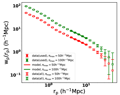
Figure 1: Comparisons of measured and model projected 2PCFs at different $r_{\rm\pi,max}$ for Mock I. Red (green) filled squares with errorbars are the measurements for $r_{\rm\pi,max}=50(100)\>h^{-1}{\rm{Mpc}}$, and the model predictions are shown as solid lines. The open squares are measurements for all scale, shown as a reference.

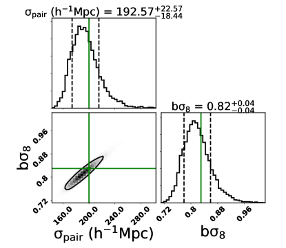
Figure 2: The 2D contours and 1D distribution of the parameters $\sigma_{\rm pair}$ and $b\sigma_{8}$ for Mock I. The black solid line in the contour corresponds to the 68.3% confidence region. The vertical black dashed lines represent the 68.3% confidence ranges for both parameters. The median and 68.3% confidence ranges are also labeled on top of the figure. The green solid lines are the input model parameters.

4 Results

In this section, we show the testing results of our method on Mocks I, II, and III. To measure the projected 2PCF $w_{\rm p}(r_{\rm p}|r_{\rm\pi,max})$, we adopt 24 logarithmic $r_{\rm p}$bins in $-0.6<\log(r_{\rm p}/\>h^{-1}{\rm{Mpc}})<1.7$ and linear bins in $r_{\pi}$ with $\Delta r_{\pi}=2\>h^{-1}{\rm{Mpc}}$ from $0$ to $r_{\rm\pi,max}=50$ and $100\>h^{-1}{\rm{Mpc}}$. The error covariance matrix for $w_{\rm p}$ is estimated from using the jackknife resampling method with 100 subsamples (see e.g., Zehavi et al., 2011; Guo et al., 2013; Xu et al., 2016, 2018). We note that the error covariance between the projected 2PCF measurements with different $r_{\rm\pi,max}$ values have been taken into account.

We adopt a Markov Chain Monte Carlo (MCMC) method to explore the parameter space using the $\chi^{2}$ that is defined as,

$$\chi^{2} = (\bm{w_{\rm p}^{\rm obs}}-\bm{w^{\rm mod}_{\rm p}})^{\mathbf{T}}{\bm{C}^{-1}}(\bm{w_{\rm p}^{\rm obs}}-\bm{w^{\rm mod}_{\rm p}})$$ (10)

$$+(n_{\rm g}^{\rm obs}-n_{\rm g}^{\rm mod})^{2}/\sigma_{n_{\rm g}}^{2}\,,$$

where ${\bm{C}}$ is the error covariance matrix of the data vector. $\bm{w_{\rm p}}$ includes the measurements with two sets of different $r_{\rm\pi,max}$ values, i.e., $\bm{w_{\rm p}}$=[$\bm{w_{\rm p}}(\bm{r_{\rm p}}|r_{\rm\pi,max1})$, $\bm{w_{\rm p}}(\bm{r_{\rm p}}|r_{\rm\pi,max2})$]. The scatter $\sigma_{n_{\rm g}}$ of the galaxy sample number density $n_{\rm g}$ is also estimated with the jackknife resampling method. The quantity with subscripts of “obs” and “mod” are for the observed and model measurements, respectively. Here we place flat priors on the input parameters, with broad parameter ranges. For example, the priors on $b\sigma_{8}$ and $\sigma_{\rm pair}$ in Mock I are $[0,8.3]$ and $[0,1000]$, respectively. Since in Mock I, we only have two free parameters, we run 30 MCMC chains, each with 20,000 steps, while for Mock II and III we run 50,000 steps due to their more free parameters. Most of the chains converge within the first 20% of steps. These first steps are regarded as burn-in stage and removed from our chains. In order to suppress the correlation between neighboring models in each chain, we thin the chain by a factor 10. This results in final MCMCs consisting of about 48,000 and 120,000 independent models that sample the posterior distributions for Mock I and II (III), respectively.

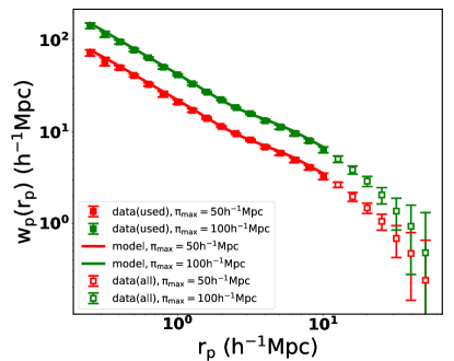
Figure 3: Similar to Figure 1, but for Mock II.

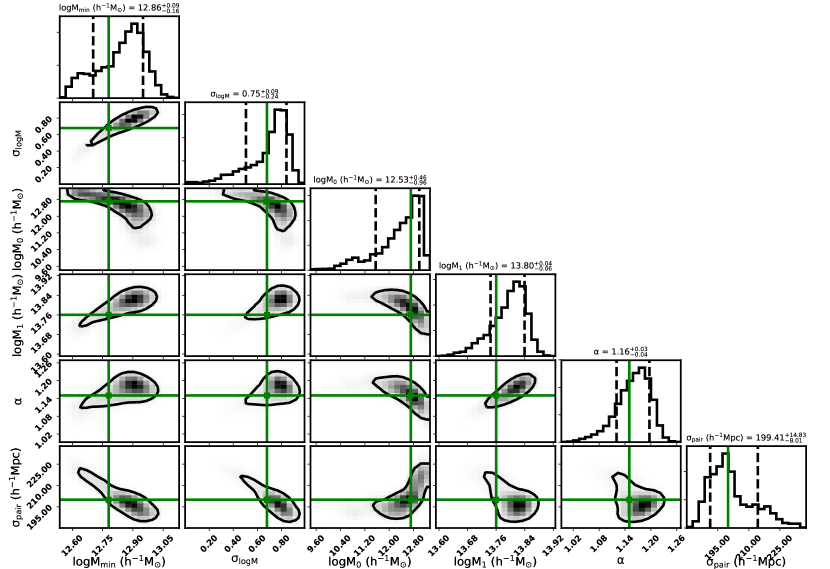
Figure 4: Simiar to Figure 2, but for the joint probability distributions of the HOD parameters and $\sigma_{\rm pair}$ for Mock II. The best-fitting model parameters with the 1$\sigma$ ranges are also labels.

4.1 Mock I: Large-scale Galaxy Bias

In Mock I, we randomly select the dark matter particles to represent galaxies in order to check whether we can recover the correct galaxy bias $b$ and photometric redshift error $\sigma_{\rm pair}$. Therefore, we only use the $w_{\rm p}$ measurements at relatively large scales of $4<r_{\rm p}<10\>h^{-1}{\rm{Mpc}}$, shown as the filled squares in Figure 1). We exclude the measurements on larger scales due to their low signal-to-noise ratios.

It is clearly shown in Figure 1 that $w_{\rm p}$ measurements with $r_{\rm\pi,max}=100\>h^{-1}{\rm{Mpc}}$ have much higher clustering amplitudes compared to those with $r_{\rm\pi,max}=50\>h^{-1}{\rm{Mpc}}$, implying that the measurements of $w_{\rm p}$ are not converged with relatively small values of $r_{\rm\pi,max}$. Especially in the situation of the large photometric redshift errors, galaxy pairs with large LOS distances still have a significant contribution to the clustering measurements. It emphasizes the importance of integrating to a extremely large $r_{\rm\pi,max}$ for traditional $w_{\rm p}$ measurements. While in our method, we can use such differences in the clustering measurements to estimate $\sigma_{\rm pair}$.

For this simplest mock, we have only two free parameters of $b\sigma_{8}$ and $\sigma_{\rm pair}$ as in Eqs. (2) and (5). We show the best-fitting model predictions of $w_{\rm p}(r_{\rm p})$ as the solid lines in Fig. 1. The joint probability distribution of $\sigma_{pair}$ and $b\sigma_{8}$ is shown in Fig. 2. The input model parameters (green horizontal and vertical lines) are very well recovered within the 1$\sigma$ parameter distributions, demonstrating the validity of our method.

4.2 Mock II: HOD Model Parameters

In Mock II, as we have assigned galaxies to halos using the HOD model, we have five HOD model parameters and an additional one of $\sigma_{\rm pair}$. To include the small-scale information in this mock to constrain the HOD model, we use the $w_{\rm p}$ measurements with $0.25\>h^{-1}{\rm{Mpc}}<r_{\rm p}<10\>h^{-1}{\rm{Mpc}}$, i.e. we have 17 data points of $w_{\rm p}$ for each $r_{\rm\pi,max}$. The best-fitting model and joint probability distributions of the model parameters are shown in Figures 3 and 4, respectively.

All of the HOD model parameters are reasonably recovered within the 1$\sigma$ probability distributions. We also note that the recovered $\sigma_{\rm pair}$ is in remarkable agreement with the input parameter, making our method a promising way of constraining the HOD, as well as testing the accuracy of photometric redshifts.

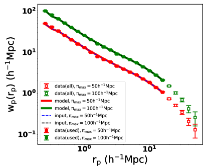
Figure 5: Similar to Figure 3, but for Mock III. For comparison, we also show the HOD model predictions with the input parameters as the dotted lines of different colors.

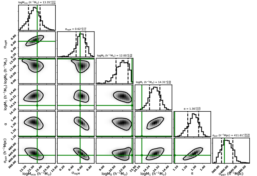
Figure 6: Similar to Fig. 4, but for Mock III.

4.3 Mock III: More Realistic Case

Now we turn to the much more realistic Mock III. The best-fitting model and joint probability distributions are shown in Figures 5 and 6, respectively. The two model parameters for the central galaxy occupation number, $M_{\rm min}$ and $\sigma_{\log M}$, are well recovered as in the case of Mock II. However, the best-fitting model parameters for satellite galaxies are not well recovered. It overpredicts the satellite occupation parameters of $M_{0}$ and $M_{1}$ and underpredicts that of $\alpha$.

To figure out the origin of such a discrepancy, we compare the best-fitting $w_{\rm p}(r_{\rm p})$ to the model predictions using the input HOD parameters (over-plotted as the thin lines in Fig  5), and find that they are almost indistinguishable with each other. Since Mock III adopts the HOD parameters from Zehavi et al. (2011) for the very luminous galaxies of $M_{r}<-21.5$, where the satellite galaxy fraction is only 9%, the strong degeneracy between the satellite HOD parameters make it difficult to exactly recover the input model parameters. Meanwhile, the central galaxy occupation parameters can still be well constrained from the clustering measurements, as well as the photometric errors.

Rather than the HOD parameters, we show in Figure 7 the direct comparisons between the observed and model occupation functions for both central and satellite galaxies. Here we do see that both the central and satellite galaxy occupation functions are well recovered with respect to their input ones. It is therefore important to emphasize that in the HOD model constraints using clustering measurements, it would be safer to compare the HOD functions rather than individual parameters.

In summary, with the above three mock tests, we demonstrate that by measuring $w_{\rm p}(r_{\rm p})$ at different $r_{\rm\pi,max}$ values in the photometric redshift surveys, we are able to reasonably constrain the HOD models as well as provide independent constraint on the overall photometric redshift error.

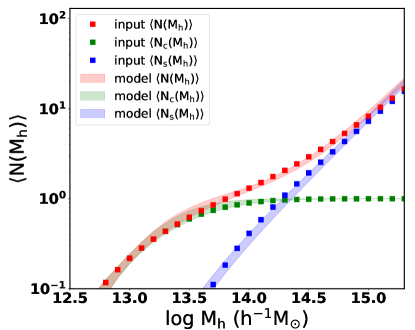
Figure 7: Comparison between input (filled squares) halo occupation functions and those of the 1$\sigma$ distributions of the model predictions (shaded regions). We show the occupation functions for all (red), central (green) and satellite (blue) galaxies, respectively.

5 Conclusions and Discussions

In this paper, we develop a method to simultaneously constrain the large-scale galaxy bias, the HOD models, and photometric redshift uncertainty by joint modeling the projected 2PCFs with multiple integration depths along the LOS direction. With the assumption that the difference between the photometric and true redshifts of galaxies follow a Gaussian distribution, we are able to model the observed projected 2PCFs in photometric redshift surveys under the HOD model framework.

We have tested our method in three mock galaxy catalogs at different complexity levels: (1) Mock I is constructed by randomly selecting the dark matter particles to represent galaxies; (2) In Mock II, we assign galaxies to halos in the simulation box using a set of HOD model parameters; (3) In Mock III, we select galaxies in a fixed light cone, introduce larger photometric redshift errors, and even include 10% catastrophic redshift measurement errors. The best-fitting models in all three mocks agree reasonably well with the input model parameters. The recovered photometric redshift errors are in very good agreement with the expected values, making our method an independent test of the accuracy of the photometric redshifts in the survey pipeline output. It is especially promising that our method can recover the HOD model parameters with a reasonable accuracy from using only the photometric galaxy samples.

Myers et al. (2009) proposed a method to infer the projected two-point cross-correlation function between a photometric sample and a spectoscopic sample by using the probability distribution function of the photometric redshifts, which significantly enhances the clustering signal. Hickox et al. (2011) further applied this method to the quasar clustering in the Boötes multi-wavelength survey. Such a method is useful when large spectroscopic samples are available at the redshifts of interest. However, high-redshift galaxy samples with spectroscopic redshifts are usually limited in sample size and area. Therefore, our method focuses on the auto-correlation function within the photometric samples and we adopt a forward modeling way to account for the photometric redshift uncertainties in the halo model rather than recovering the intrinsic real-space correlation function from observation.

Cowley et al. (2018) proposed a similar Gaussian error kernal in their modeling of angular galaxy clustering measurements incorporated with photometric redshift errors. Compared to the traditional halo modeling of the galaxy angular clustering measurements, the main advantage of modeling the projected 2PCF in the photometric redshift surveys is that the redshift extent in angular clustering measurements is usually much larger than the photometric redshift errors, which leads to a large projection effect, reducing the number of effective modes and thus weakening the constraints on the galaxy-halo connection. Moreover, modeling the projected 2PCF is much simpler than the angular one, where the conversion from the real-space 2PCF to the angular one is necessary (see e.g., Coupon et al., 2012; Cowley et al., 2018). Due to the strong correlation between $\sigma_{\rm pair}$ and $b\sigma_{8}$, the photometric redshift error can be better constrained in our modeling of the projected 2PCF.

At the moment, there are many finished and on-going galaxy photometric surveys with various depths, e.g., the Canada-France-Hawaii Telescope Legacy Survey (CFHTLS; Cuillandre et al., 2012), the Dark Energy Survey (DES; Abbott et al., 2018), the Kilo-Degree Survey (KiDS; de Jong et al., 2013), the The Dark Energy Camera Legacy Survey (DECaLS; Dey et al., 2018), the Hyper Suprime-Cam (HSC; Miyazaki et al., 2012), as well as the next-generation surveys, such as the Large Synoptic Survey Telescope (LSST; Graham et al., 2018). Our method is potentially very useful for understanding the galaxy-halo connection at different cosmic epochs with these large-scale galaxy photometric surveys.

However, we also note that we have assumed a simple Gaussian form for the photometric redshift error. It is possibly different from the real distribution of the photometric redshift errors in the surveys. For example, Guo et al. (2015) found that the redshift error in SDSS in fact follows a Gaussian-convolved Laplace distribution. But the Gaussian distribution can still be used as a first-order approximation as shown in Moutard et al. (2016) and Cowley et al. (2018). Our model can be further improved in future by taking into account the fact that the photometric redshift error may be dependent on the galaxy luminosity and redshift. By incorporating the simulation-based halo modeling method as proposed in Zheng & Guo (2016), we will be able to provide more accurate constraints to the HOD parameters, which will be explored in a subsequent paper of applying our method to the real photometric surveys (Xu et al. in preparation).

References

- Abazajian et al. (2009) Abazajian, K. N., Adelman-McCarthy, J. K., Agüeros, M. A., et al. 2009, ApJS, 182, 543
- Abbott et al. (2018) Abbott, T. M. C., Abdalla, F. B., Allam, S., et al. 2018, ArXiv e-prints, arXiv:1801.03181
- Behroozi et al. (2010) Behroozi, P. S., Conroy, C., & Wechsler, R. H. 2010, ApJ, 717, 379
- Behroozi et al. (2013) Behroozi, P. S., Wechsler, R. H., & Wu, H.-Y. 2013, ApJ, 762, 109
- Berlind & Weinberg (2002) Berlind, A. A., & Weinberg, D. H. 2002, ApJ, 575, 587
- Chaves-Montero et al. (2016) Chaves-Montero, J., Angulo, R. E., Schaye, J., et al. 2016, MNRAS, 460, 3100
- Chen et al. (2018) Chen, Y., Mo, H., Li, C., et al. 2018, ArXiv e-prints, arXiv:1809.00523
- Coil et al. (2004) Coil, A. L., Davis, M., Madgwick, D. S., et al. 2004, ApJ, 609, 525
- Coil et al. (2008) Coil, A. L., Newman, J. A., Croton, D., et al. 2008, ApJ, 672, 153
- Colless et al. (2001) Colless, M., Dalton, G., Maddox, S., et al. 2001, MNRAS, 328, 1039
- Conroy et al. (2006) Conroy, C., Wechsler, R. H., & Kravtsov, A. V. 2006, ApJ, 647, 201
- Cooray (2006) Cooray, A. 2006, MNRAS, 365, 842
- Coupon et al. (2012) Coupon, J., Kilbinger, M., McCracken, H. J., et al. 2012, A&A, 542, A5
- Cowley et al. (2018) Cowley, W. I., Caputi, K. I., Deshmukh, S., et al. 2018, ApJ, 853, 69
- Cuillandre et al. (2012) Cuillandre, J.-C. J., Withington, K., Hudelot, P., et al. 2012, in Observatory Operations: Strategies, Processes, and Systems IV, Vol. 8448, 84480M
- Davis et al. (1985) Davis, M., Efstathiou, G., Frenk, C. S., & White, S. D. M. 1985, ApJ, 292, 371
- de Jong et al. (2013) de Jong, J. T. A., Verdoes Kleijn, G. A., Kuijken, K. H., & Valentijn, E. A. 2013, Experimental Astronomy, 35, 25
- Dey et al. (2018) Dey, A., Schlegel, D. J., Lang, D., et al. 2018, ArXiv e-prints, arXiv:1804.08657
- Eisenstein et al. (2005) Eisenstein, D. J., Zehavi, I., Hogg, D. W., et al. 2005, ApJ, 633, 560
- Graham et al. (2018) Graham, M. L., Connolly, A. J., Ivezić, Ž., et al. 2018, AJ, 155, 1
- Guo et al. (2018) Guo, H., Yang, X., & Lu, Y. 2018, ApJ, 858, 30
- Guo et al. (2013) Guo, H., Zehavi, I., Zheng, Z., et al. 2013, ApJ, 767, 122
- Guo et al. (2014) Guo, H., Zheng, Z., Zehavi, I., et al. 2014, MNRAS, 441, 2398
- Guo et al. (2015) —. 2015, MNRAS, 453, 4368
- Guo et al. (2016) Guo, H., Zheng, Z., Behroozi, P. S., et al. 2016, MNRAS, 459, 3040
- Guo & White (2014) Guo, Q., & White, S. 2014, MNRAS, 437, 3228
- Guo et al. (2010) Guo, Q., White, S., Li, C., & Boylan-Kolchin, M. 2010, MNRAS, 404, 1111
- Guo et al. (2011) Guo, Q., White, S., Boylan-Kolchin, M., et al. 2011, MNRAS, 413, 101
- Guzzo et al. (2014) Guzzo, L., Scodeggio, M., Garilli, B., et al. 2014, A&A, 566, A108
- Han et al. (2012) Han, J., Jing, Y. P., Wang, H., & Wang, W. 2012, MNRAS, 427, 2437
- Harikane et al. (2016) Harikane, Y., Ouchi, M., Ono, Y., et al. 2016, ApJ, 821, 123
- Harikane et al. (2018) —. 2018, Publications of the Astronomical Society of Japan, 70, S11
- He et al. (2018) He, W., Akiyama, M., Bosch, J., et al. 2018, Publications of the Astronomical Society of Japan, 70, S33
- Hickox et al. (2011) Hickox, R. C., Myers, A. D., Brodwin, M., et al. 2011, ApJ, 731, 117
- Jiang & van den Bosch (2014) Jiang, F., & van den Bosch, F. C. 2014, MNRAS, 440, 193
- Jing (2018) Jing, Y. P. 2018, ArXiv e-prints, arXiv:1807.06802
- Jing et al. (1998) Jing, Y. P., Mo, H. J., & Börner, G. 1998, ApJ, 494, 1
- Jing et al. (2007) Jing, Y. P., Suto, Y., & Mo, H. J. 2007, ApJ, 657, 664
- Kang et al. (2005) Kang, X., Jing, Y. P., Mo, H. J., & Börner, G. 2005, ApJ, 631, 21
- Katz et al. (1996) Katz, N., Weinberg, D. H., & Hernquist, L. 1996, ApJS, 105, 19
- Kauffmann et al. (1993) Kauffmann, G., White, S. D. M., & Guiderdoni, B. 1993, MNRAS, 264, 201
- Klypin et al. (2016) Klypin, A., Yepes, G., Gottlöber, S., Prada, F., & Heß, S. 2016, MNRAS, 457, 4340
- Lewis et al. (2000) Lewis, A., Challinor, A., & Lasenby, A. 2000, ApJ, 538, 473
- Li et al. (2006) Li, C., Kauffmann, G., Jing, Y. P., et al. 2006, MNRAS, 368, 21
- Lu et al. (2017) Lu, Y., Benson, A., Wetzel, A., et al. 2017, ApJ, 846, 66
- Masjedi et al. (2006) Masjedi, M., Hogg, D. W., Cool, R. J., et al. 2006, ApJ, 644, 54
- Miyazaki et al. (2012) Miyazaki, S., Komiyama, Y., Nakaya, H., et al. 2012, in Ground-based and Airborne Instrumentation for Astronomy IV, Vol. 8446, 84460Z
- Mo et al. (2010) Mo, H., van den Bosch, F. C., & White, S. 2010, Galaxy Formation and Evolution
- Moutard et al. (2016) Moutard, T., Arnouts, S., Ilbert, O., et al. 2016, A&A, 590, A102
- Myers et al. (2009) Myers, A. D., White, M., & Ball, N. M. 2009, MNRAS, 399, 2279
- Navarro et al. (1997) Navarro, J. F., Frenk, C. S., & White, S. D. M. 1997, ApJ, 490, 493
- Parkinson et al. (2008) Parkinson, H., Cole, S., & Helly, J. 2008, MNRAS, 383, 557
- Rodríguez-Puebla et al. (2015) Rodríguez-Puebla, A., Avila-Reese, V., Yang, X., et al. 2015, ApJ, 799, 130
- Seljak & Zaldarriaga (1996) Seljak, U., & Zaldarriaga, M. 1996, ApJ, 469, 437
- Shi et al. (2016) Shi, F., Yang, X., Wang, H., et al. 2016, ApJ, 833, 241
- Simha et al. (2012) Simha, V., Weinberg, D. H., Davé, R., et al. 2012, MNRAS, 423, 3458
- Springel et al. (2005) Springel, V., et al. 2005, Nature, 435, 629
- Szapudi & Szalay (1998) Szapudi, I., & Szalay, A. S. 1998, ApJ, 494, L41
- Vale & Ostriker (2006) Vale, A., & Ostriker, J. P. 2006, MNRAS, 371, 1173
- van den Bosch et al. (2013) van den Bosch, F. C., More, S., Cacciato, M., Mo, H., & Yang, X. 2013, MNRAS, 430, 725
- van den Bosch et al. (2007) van den Bosch, F. C., Yang, X., Mo, H. J., et al. 2007, MNRAS, 376, 841
- Vogelsberger et al. (2014) Vogelsberger, M., Genel, S., Springel, V., et al. 2014, MNRAS, 444, 1518
- Wang et al. (2011) Wang, W., Jing, Y. P., Li, C., Okumura, T., & Han, J. 2011, ApJ, 734, 88
- Wechsler & Tinker (2018) Wechsler, R. H., & Tinker, J. L. 2018, ArXiv e-prints, arXiv:1804.03097
- White & Rees (1978) White, S. D. M., & Rees, M. J. 1978, MNRAS, 183, 341
- Xu et al. (2016) Xu, H., Zheng, Z., Guo, H., Zhu, J., & Zehavi, I. 2016, MNRAS, 460, 3647
- Xu et al. (2018) Xu, H., Zheng, Z., Guo, H., et al. 2018, MNRAS, 481, 5470
- Yang et al. (2004) Yang, X., Mo, H. J., Jing, Y. P., van den Bosch, F. C., & Chu, Y. 2004, MNRAS, 350, 1153
- Yang et al. (2003) Yang, X., Mo, H. J., & van den Bosch, F. C. 2003, MNRAS, 339, 1057
- Yang et al. (2012) Yang, X., Mo, H. J., van den Bosch, F. C., Zhang, Y., & Han, J. 2012, ApJ, 752, 41
- York et al. (2000) York, D. G., Adelman, J., Anderson, Jr., J. E., et al. 2000, AJ, 120, 1579
- Yuan et al. (2018) Yuan, S., Eisenstein, D. J., & Garrison, L. H. 2018, MNRAS, 478, 2019
- Zehavi et al. (2005) Zehavi, I., et al. 2005, ApJ, 630, 1
- Zehavi et al. (2011) Zehavi, I., Zheng, Z., Weinberg, D. H., et al. 2011, ApJ, 736, 59
- Zheng et al. (2007) Zheng, Z., Coil, A. L., & Zehavi, I. 2007, ApJ, 667, 760
- Zheng & Guo (2016) Zheng, Z., & Guo, H. 2016, MNRAS, 458, 4015
- Zheng et al. (2005) Zheng, Z., Berlind, A. A., Weinberg, D. H., et al. 2005, ApJ, 633, 791
- Zu & Mandelbaum (2015) Zu, Y., & Mandelbaum, R. 2015, MNRAS, 454, 1161
- Zu & Mandelbaum (2016) —. 2016, MNRAS, 457, 4360
- Zu & Mandelbaum (2018) —. 2018, MNRAS, 476, 1637