Charge transfer statistics and qubit dynamics at tunneling Fermi-edge singularity.

Abstract

Tunneling of spinless electrons from a single-channel emitter into an empty collector through an interacting resonant level of the quantum dot (QD) is studied, when all Coulomb screening of charge variations on the dot is realized by the emitter channel and the system is mapped onto an exactly solvable model of a dissipative qubit. In this model we describe the qubit density matrix evolution with a generalized Lindblad equation, which permit us to count the tunneling electrons and therefore relate the qubit dynamics to the charge transfer statistics. In particular, the coefficients of its generating function equal to the time dependent probabilities to have the fixed number of electrons tunneled into the collector are expressed through the parameters of a non-Hermitian Hamiltonian evolution of the qubit pure states in between the successive electron tunnelings. From the long time asymptotics of the generating function we calculate Fano factors of the second and third order (skewness) and establish their relation to the extra average and cumulant, respectively, of the charge accumulated in the transient process of the empty QD evolution beyond their linear time dependence. It explains the origin of the sub and super Poisson shot noise in this system and shows that the super Poisson signals existence of a non-monotonous oscillating transient current and the qubit coherent dynamics. The mechanism is illustrated with particular examples of the generating functions, one of which coincides in the large time limit with the $1/3$ fractional Poissonian realized without the real fractional charge tunneling.

I Introduction

The Fermi-edge singularity (FES) resulting 1 ; 2 from the reconstruction of the Fermi sea of conduction electrons under a sudden change of a local potential have been primarily observed 3 ; 4 as a power-law singularity in X-ray absorption spectra. A similar phenomenon of the FES in transport of spinless electrons through a quantum dot (QD) was predicted 5 in the perturbative regime when a localized QD level is below the Fermi level of the emitter in its proximity and the collector is effectively empty (or in equivalent formulation through the particle-hole symmetry) and the tunneling rate of the emitter is sufficiently small. Then, the subsequent separated in time electron tunnelings from the emitter vary the localized level charge and generate sudden changes of the scattering potential leading to the FES in the I-V curves at the voltage threshold corresponding to the resonance. Direct observation of these perturbative results in experiments geim ; 6 ; 7 ; 8 ; 9 ; lar , however, is complicated due to the uncontrolled effects such as of a finite life time of the electrons (the level broadening of the QD localized state), temperature smearing and variation of tunneling parameters due to application of the bias voltage. Therefore, it has been suggested epl that the true FES nature of a threshold peak in the I-V dependence can be verified through observation of the oscillatory behavior of a corresponding time-dependent transient current. Indeed, in the FES theory 1 ; 2 appearance of such a threshold peak signals formation of a two-level system of the exciton electron-hole pair or qubit in the tunneling channel at the QD. The qubit undergoes dissipative dynamics characterized L ; Sch , in the absence of the collector tunneling, by the oscillations of the levels occupation. It should create an oscillating transient current at least for a weak enough collector tunneling rate. Although a direct observation of these oscillations would give the most clear verification of the nature of the I-V threshold peaks, it involves measurement of the time dependent transient current averaged over its quantum fluctuations, which is a challenging experimental task. In the recent experiments 8 ; noise ; noise2 the low-temperature short noise measurements have been carried out for this purpose. These measurements showed existence of the sub and super Poisson statistics of the current fluctuations at the FES and have raised 8 ; noise a new interest novotny in the qubit dynamics, though their coherency manifestation in the current fluctuations needs to be further clarified. Also, for this purpose the methods of measurement of the third order current cumulants shovkun ; third could be considered.

Therefore, in this work we study quantum fluctuations of the charge transferred into collector and their reflection of the coherent qubit dynamics in the FES regime in the simplified, but still realistic setup suggested earlier epl ; prb , in which all Coulomb screening of sudden charge variations on the QD during the spinless electron tunneling is due to a single tunneling channel of the emitter. It can be realized, in particular, if the emitter is represented by a single edge-state in the integer quantum Hall effect. This system is described by a non-equilibrium model of an interacting resonant level, which can be mapped epl onto an exactly solvable model of a dissipative qubit. Making use of its solution it was demonstrated earlier that FES in the I-V dependence in this system is accompanied for a wide range of the model parameters by an oscillating behavior epl of the collector transient current, in particular, when the QD evolves from its empty state and that the qubit dynamics also manifest themselves through the resonant features of the a.c. response prb .

Here we further study quantum fluctuations of the charge transfer in this model by applying the method of full counting statistics lll ; naz . For this purpose we derive a generalized Lindblad equation, which describes the qubit density matrix evolution and simultaneouly permit us to count the tunneling electrons and therefore relate the qubit dynamics to the charge transfer statistics. From this equation it follows that the generating function of the charge transfer in an arbitrary evolution process can be expressed through the generating function for the process initiating from the empty QD. The latter is found by dividing the whole process of the qubit evolution into separate time intervals between the successive electron tunnelings. In these intervals dynamics of the qubit pure states are governed by a non-Hermitian Hamiltonian. The coefficients of the generating function equal to the time dependent probabilities to have the corresponding fixed number of electrons tunneled into the collector are determined by matrix elements of the non-Hermitian Hamiltonian evolution operator and therefore can be used to extract from them the parameters of this evolution (the frequencies and the damping rates).

From the linear in time part of the long time asymptotics of the generating function logarithm or cumulant generating function (CGF) we calculate the zero-frequency reduced current correlators commonly studied in the full counting statistics. Normalized by the average stationary current, the second order correlator known as Fano factor $F_{2}$ predicts existence in this system the parametrical regions of the sub Poisson short noise $F_{2}<1$ around the resonance and the super Poisson noise $F_{2}>1$ far from the resonance. Among the generalized higher order Fano factors given by the normalized higher order current correlators we examine the third one called skewness and find a small parametric area, where it changes its sign and becomes negative.

We also study the next order finite term of the CGF long time asymptotics, which determines the extra charge accumulation in the transient process, in particular, of the empty QD evolution beyond the one characterized by the linear in time cumulants. We establish a direct relation between the Fano factor and the extra charge average and between the skewness and the extra charge cumulants. This relation explains the origin of the sub and super Poisson shot noise in this system and shows that the super Poissonian means existence of a non-monotonous oscillating transient current as a consequence of the qubit coherent dynamics.

The mechanism is illustrated with particular examples of the generating functions in the special regimes, one of which coincides in the large time limit with the $1/3$ fractional Poissonian realized without the real fractional charge tunneling. This example underlines that observation of the fractional charge in the Poissonian short noise is necessary, but not sufficient to prove its real tunneling.

The paper is organized as follows. In Sec. II we introduce the model and formulate those conditions, which make it solvable through a standard mapping onto the dissipative two-level system or qubit. In Sec. III we apply the non-equilibrium Keldysh technique to derive the generalized Lindbladian equation describing the dissipative evolution of the qubit density matrix and counting the charge transferred into the collector. Its properties are studied. In particular, we find its stationary solution and the stationary tunneling current and derive a simple relation between the generating functions of the charge transfer during the two processes initiating from the empty and stationary state of the QD as a special case of the general expression for generating function for an arbitrary evolution process through the one for the process initiating from the empty QD.

In Sec. IV we consider the non-Hermitian Hamiltonian evolution of the qubit two-level system in between the successive electron tunneling. Both two-level energies modified by the collector tunneling rate acquire in general different imaginary parts. We find the evolution operator and use its matrix elements to calculate the generating function for the empty QD evolution. Its coefficients are studied to relate the time dependence of probabilities to find the corresponding fixed number of electrons tunneled into the collector to the qubit evolution.

In Sec. V we calculate the zero-frequency reduced current correlators (or current cumulants) defined by the leading exponent of the generating function independent of the QD initial state and discuss behavior of the Fano factor and skewness. We also find the extra average and second order cumulant of the charge accumulated in the process of the empty QD evolution which are defined by the prefactor of the leading exponent. It turns out that the Fano factors and the extra charge moments are not independent. To establish connection between them we make use of the above relation between the two generating functions.

In Section VI two generating functions are calculated asymptotically in the two regimes when amplitude of the qubit two-level coupling is much smaller than the collector tunneling rate or the absolute value of the QD level energy and in the opposite limit when the amplitude is much larger than both of them. Accumulation of the extra charge in these regimes is illustrated with the corresponding transient current behavior. We also calculate the generating function at the special point of degeneracy of the two qubit levels energies including their imaginary parts. We find that in this special case it takes the $1/3$ fractional Poissonian form, where all probabilities of tunneling of the fractional charges mean tunneling of the charges integer parts. The large time limit of this function nontheless coincides with the true $1/3$ fractional Poisson. This example underlines that observation of the fractional charge in the Poissonian short noise is necessary, but not sufficient to prove its real tunneling. The results of the work are summarized in the Conclusion.

II Model

The system we consider below is described with Hamiltonian $\mathcal{H}=\mathcal{H}_{res}+\mathcal{H}_{C}$ consisting of the one-particle Hamiltonian of resonant tunneling of spinless electrons and the Coulomb interaction between instant charge variations of the dot and electrons in the emitter. The resonant tunneling Hamiltonian takes the following form

$$\mathcal{H}_{res}=-\epsilon_{d}d^{+}d+\sum_{a=e,c}\mathcal{H}_{0}[\psi_{a}]+w_{a}(d^{+}\psi_{a}(0)+h.c.)\ ,$$ (1)

where the first term represents the resonant level of the dot, whose energy is $-\epsilon_{d}$. Electrons in the emitter (collector) are described with the chiral Fermi fields $\psi_{a}(x),a=e(c)$, whose dynamics is governed by the Hamiltonian $\mathcal{H}_{0}[\psi]==-i\!\!\int\!dx\psi^{+}(x)\partial_{x}\psi(x)\ (\hbar=1)$ with the Fermi level equal to zero or drawn to $-\infty$, respectively, and $w_{a}$ are the correspondent tunneling amplitudes. The Coulomb interaction in the Hamiltonian $\mathcal{H}$ is introduced as

$$\mathcal{H}_{C}=U_{C}\psi_{e}^{+}(0)\psi_{e}(0)(d^{+}d-1/2)\ .$$ (2)

Its strength parameter $U_{C}$ defines the scattering phase variation $\theta$ for electrons in the emitter channel and therefore the change of the localized charge in the emitter $\delta n=\theta/\pi\ \ (e=1)$, which we assume provides the perfect screening of the QD charge: $\delta n=-1$.

After implementation of bosonization of the emitter Fermi field $\psi_{e}(x)=\sqrt{\frac{D}{2\pi}}\eta e^{i\phi(x)}$, where $\eta$ denotes an auxiliary Majorana fermion, $D$ is the large Fermi energy of the emitter, and the chiral Bose field $\phi(x)$ satisfies $[\partial_{x}\phi(x),\phi(y)]=i2\pi\delta(x-y)$, and further completion of a standard rotation schotte , under the above screening assumption we have transformed epl $\mathcal{H}$ into the Hamiltonian of the dissipative two-level system or qubit:

$$\mathcal{H}_{Q} = -\epsilon_{d}d^{+}d+\mathcal{H}_{0}[\psi_{c}]+w_{c}(\psi_{c}^{+}(0)e^{i\phi(0)}d+h.c.)$$ (3)

$$+\Delta\eta(d-d^{+})\ ,$$

where $\Delta=\sqrt{\frac{D}{2\pi}}w_{e}$ and the time dependent correlator of electrons in the empty collector $\langle\psi_{c}(t)\psi_{c}^{+}(0)\rangle=\delta(t)$ will allow us to drop the bosonic exponents in the third term on the right-hand side in (3).

III Lindblad equation for the qubit evolution and count of tunneling charge

We use this Hamiltonian to describe the dissipative evolution of the qubit density matrix $\rho_{a,b}(t)$, where $a,b=0,1$ denote the empty and filled levels, respectively. In the absence of the tunneling into the collector at $w_{c}=0$, $\mathcal{H}_{Q}$ in Eq. (3) transforms through the substitutions of $\eta(d-d^{+})=\sigma_{1}$ and $d^{+}d=(1-\sigma_{3})/2$ ( $\sigma_{1,3}$ are the corresponding Pauli matrices) into the Hamiltonian $\mathcal{H}_{S}$ of a spin $1/2$ rotating in the magnetic field $\mathbf{h}=(2\Delta,0,\epsilon_{d})^{T}$ with the frequency $\omega_{0}=\sqrt{4\Delta^{2}+\epsilon_{d}^{2}}$ . Then the evolution equation follows from

$$\partial_{t}\rho(t)=i[\rho(t),\mathcal{H}_{S}]\ .$$ (4)

To incorporate in it the dissipation effect due to tunneling into the empty collector we apply the diagrammatic perturbative expansion of the S-matrix defined by the Hamiltonian (3) in the tunneling amplitudes $w_{e,c}$ in the Keldysh technique konig . This permits us to integrate out the collector Fermi field in the following way. At an arbitrary time $t$ each diagram ascribes indexes $a(t_{+})$ and $b(t_{-})$ of the qubit states to the upper and lower branches of the time-loop Keldysh contour. This corresponds to the qubit state characterized by the $\rho_{a,b}(t)$ element of the density matrix. The expansion in $w_{e}$ produces two-leg vertices in each line, which change the line index into the opposite one. Their effect on the density matrix evolution has been already included in Eq. (4). In addition, each line with index $1$ acquires two-leg diagonal vertices produced by the electronic correlators $\langle\psi_{c}(t_{\alpha})\psi_{c}^{+}(t_{\alpha}^{\prime})\rangle,\ \alpha=\pm$. They result in the additional contributions to the density matrix variation: $\Delta\partial_{t}\rho_{10}(t)=-\Gamma\rho_{10}(t),\ \Delta\partial_{t}\rho_{01}(t)=-\Gamma\rho_{01}(t),\ \Delta\partial_{t}\rho_{11}(t)=-2\Gamma\rho_{11}(t),\ \Gamma=w_{c}^{2}/2$. Next, to count the electron tunnelings into the collector we ascribe lll the opposite phases to the collector tunneling amplitude $w_{c}\exp\{\pm i\chi/2\}$ along the upper and lower Keldysh contour branch, correspondingly. These phases do not affect the above contributions, which do not mix the amplitudes of the the different branches. Then there are also vertical fermion lines from the upper branch to the lower one due to the non-vanishing correlator $\langle\psi_{c}(t_{-})\psi_{c}^{+}(t_{+}^{\prime})\rangle$, which lead to the variation affected by the phase difference as follows $\Delta\partial_{t}\rho_{00}(t)=2\Gamma w\rho_{11}(t),\ w=\exp\{i\chi\}$. Incorporating these additional terms into Eq. (4) we come to the Lindblad quantum master equation

$$\partial_{t}\rho(t,w) = i[\rho,\mathcal{H}_{S}]-\Gamma|1\rangle\langle 1|\rho-\Gamma\rho|1\rangle\langle 1|$$ (5)

$$+2w\Gamma|0\rangle\langle 1|\rho|1\rangle\langle 0|.$$

for the qubit density matrix evolution and counting the charge transfer. Here the vectors $|0\rangle=(1,0)^{T}$ and $|1\rangle=(0.1)^{T}$ describe the empty and filled QD, respectively. It is exact in our model with the Hamiltonian (3) that takes into account many-body interaction of the QD with the emitter Fermi sea. In our special case $\theta=-\pi$, the Lindbladian evolution defined by the ordinary differential equation (5) does not have quantum memory. The physical reason for this behavior originates from combination of the two factors: first, the instant tunneling of electrons into the empty collector and second the perfect screening by the emitter of the QD charge variations, which leave no traces in the Fermi sea after each electron jump. Evolution of the system obeys the Born-Markov description Timm , this type of equations is well known from the theory of open quantum systems. The first three terms on the right-hand side of (5) generate the deterministic or no-jump part of the evolution that can be described with a modified von Neumann equation after inclusion of the non-Hermitian complements into $\mathcal{H}_{S}$ . The last term called recycling or jump operator counts the real electron tunneling into the collector.

Solving Eq. (5) with some initial $\rho(0)$ independent of $w$ at $t=0$, we find the generating function $P(w,t)$ by taking trace of the density matrix: $P(w,t)=Tr[\rho(w,t)]=\sum_{n=0}^{\infty}P_{n}(t)w^{n}$ and $P(w,0)=1$.

III.1 Stationary density matrix

Making use of the representation $\rho_{st}=[1+\sum_{l}a_{l}\sigma_{l}]/2$, where $\sigma_{l}],\ l=1\div 3$ are Pauli matrices, and demanding that the right-hand side of Eq. (5) at $w=1$ vanishes after substitution of $\rho_{st}$ in it, we find the stationary Bloch vector $\mathbf{a}_{\infty}$ with components $a_{l}$ as follows

$$\mathbf{a}_{\infty}=\frac{[2\epsilon_{d}\Delta,-2\Delta\Gamma,(\epsilon_{d}^{2}+\Gamma^{2})]^{T}}{\left(\epsilon_{d}^{2}+\Gamma^{2}+2\Delta^{2}\right)}\ .$$ (6)

In general, an instant tunneling current $I(t)$ into the empty collector directly measures the diagonal matrix element of the qubit density matrix us through their relation

$$I(t)=2\Gamma\rho_{11}(t,1)=\Gamma[1-a_{3}(t)]$$ (7)

It gives us the stationary tunneling current as $I_{0}=2\Gamma\Delta^{2}/(2\Delta^{2}+\Gamma^{2}+\epsilon_{d}^{2})$. Since in our model $\epsilon_{d}$ is equal to the bias voltage applied to the emitter, the current $I_{0}(\epsilon_{d})$ specifies a symmetric threshold peak in the $I-V$ dependence smeared by the finite tunneling rates and exhibiting the power decrease as $\epsilon_{d}^{-2}$ far from the threshold. At $\Gamma\gg\Delta$ this expression coincides with the perturbative results of 5 ; lar and shows the considerable growth of the maximum current $I_{0}(0)=w_{e}^{2}(D/\pi\Gamma)$ due to the Coulomb interaction.

III.2 Connection to the empty QD evolution

Since the right-hand side of Eq. (5) is the linear transformation of the density matrix we can write it in terms of the superoperator acting on the Hilbert space of matrices as

$$\partial_{t}\rho=\mathcal{L}(w)\rho=\mathcal{L}(0)\rho+2w\Gamma\mathcal{L}_{j}\rho\,,$$ (8)

where the superoperator $\mathcal{L}(w)$ linear dependence on the counting parameter $w$ is accounted for explicitly with the jump superoperator:

$$\mathcal{L}_{j}\rho\equiv|0\rangle\langle 1|\rho|1\rangle\langle 0|\,.$$ (9)

The evolution operator for the Lindblat equation takes the following form

$$e^{t\mathcal{L}(w)}=e^{t\mathcal{L}(1)}+2(w-1)\Gamma\int_{0}^{t}d\tau e^{(t-\tau)\mathcal{L}(w)}\mathcal{L}_{j}e^{\tau\mathcal{L}(1)}\,.$$ (10)

Then the Lindbladian evolution of an arbitrary initial QD state $\rho(0)=\rho_{0}$

$$\rho_{\rho_{0}}(w,t)=\rho_{\rho_{0}}(1,t)+(w-1)\int_{0}^{t}d\tau\langle I(t-\tau)\rangle_{\rho_{0}}\rho_{E}(w,\tau)$$ (11)

is connected to the evolution of the empty QD state

$$\rho_{E}(t,w)=e^{t\mathcal{L}(w)}|0\rangle\langle 0|\,.$$ (12)

via the average transient current $\langle I(t)\rangle_{\rho_{0}}$. Taking trace of both sides of (11) we find relation between their generating functions

$$P_{\rho_{0}}(w,t)=1+(w-1)\int_{0}^{t}d\tau\langle I(t-\tau)\rangle_{\rho_{0}}P(w,\tau)\,.$$ (13)

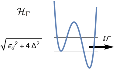
Figure 1: Two level system with the coupling parameter $\Delta$ under the bias $\epsilon_{d}$. The arrow with $i\Gamma$ illustrates tunneling from the second well.

Both relations in Eq. (11,13) simplify epl2 if the initial QD state is stationary. The first one becomes

$$\rho_{st}(w,t)=\rho_{st}(0)+(w-1)I_{0}\int_{0}^{t}d\tau\rho_{E}(w,\tau)$$ (14)

and the second after differentiating it with respect to the time can be written as

$$\partial_{t}P^{st}(t,w)=(w-1)I_{0}P(t,w)\theta(t)\ ,$$ (15)

where the Heavyside step function $\theta(t)$ starts counting the charge transfer at $t=0$. It is straightforward to see from Eq. (15) that in the steady process $\langle I\rangle_{st}=\partial_{w}\partial_{t}P^{st}(t,1)=I_{0}$ and similarly one can obtain higher order moments of steady charge transfer from this relation. Therefore, it suffices below to focus our study on the generating function $P(t,w)$ for the process starting from the empty QD.

IV Generating function and Lindblad equation

It is elucidative to derive the generating function $P(w,t)$ directly from the Lindblad equation (5). We proceed with this here by solving Eq. (5) perturbatively in the last term proportional $w$, which counts the number of electron real tunneling into the collector. In the absence of this term the evolution of qubit pure states is defined by the evolution operator $S_{0}(t)=\exp\{-i\mathcal{H}_{\Gamma}t\}$ with the non-Hermitian Hamiltonian:

$$\mathcal{H}_{\Gamma}=\Delta\sigma_{1}+(\epsilon_{d}+i\Gamma)\sigma_{3}/2-i\Gamma/2\ .$$ (16)

The non-Hermicity leads to decrease of the amplitudes of the pure state in the process of its evolution which is due to the electron tunneling processes. Then the probability of observing “no tunneling” equal to the zero term $P_{0}(t)$ of the generating function expansion reads as follows

$$P_{0}(t)=\sum_{a=0,1}P_{0}^{(a)}(t)=\sum_{a=0,1}|\langle a|S_{0}(t)|0\rangle|^{2}\ .$$ (17)

Then the generating function comes up as a perturbative series in $w$:

$$P(w,t)=P_{0}(t)+\sum_{n\geq 1}(2w\Gamma)^{n}$$

$$\times \int_{0}^{t}dt_{1}...\int_{t_{n-1}}^{t}dt_{n}P_{0}(t-t_{n})P_{0}^{(1)}(t_{n}-t_{n-1})..P_{0}^{(1)}(t_{1})\ .$$

Applying the Laplace transformation to both sides of Eq. (IV) one sums up the series and finds the generation function as follows

$$P(w,t)=\int_{C}\frac{dze^{zt}}{2\pi i}\frac{\check{P}_{0}(z)}{1-2w\Gamma\check{P}_{0}^{(1)}(z)}\ ,$$ (19)

where $\check{P}_{0}^{(a)}(z)$ stands for the Laplace transformation of $P_{0}^{(a)}(t)$.

IV.1 Qubit pure state evolution

The operator $S_{0}(t)$ specifying the qubit pure state evolution between the electron tunnelings into the collector and defined by $\mathcal{H}_{\Gamma}$ in Eq, (16) takes the following explicit form

$$S_{0}(t)=\frac{1}{2}\sum_{\pm}e^{-(\Gamma\pm\mu\mp i\omega_{e})t/2}\left[1\mp\frac{2\Delta\sigma_{1}+(\epsilon_{D}+i\Gamma)\sigma_{3}}{\omega_{e}+i\mu}\right]\ ,$$ (20)

where the parameters $\omega_{e}$ and $\mu$ are the real and imaginary parts of $\sqrt{4\Delta^{2}+(\epsilon_{D}+i\Gamma)^{2}}$ equal to

$$\omega_{e} = \sqrt{\sqrt{\Omega^{4}+4\Gamma^{2}\epsilon_{D}^{2}}+\Omega^{2}}/\sqrt{2}$$ (21)

$$\mu = \mbox{sgn}\epsilon_{D}\sqrt{\sqrt{\Omega^{4}+4\Gamma^{2}\epsilon_{D}^{2}}-\Omega^{2}}/\sqrt{2}$$ (22)

$$\mbox{where}\ \ \Omega^{2} = 4\Delta^{2}+\epsilon_{D}^{2}-\Gamma^{2}\ .$$ (23)

Note, that

$$\mu^{2}+\omega_{e}^{2}=\sqrt{\left(\epsilon_{d}^{2}+4\Delta^{2}-\Gamma^{2}\right){}^{2}+4\Gamma^{2}\epsilon_{d}^{2}}$$ (24)

The two qubit states corresponding to the energies $\pm\omega_{e}/2$ possess in general different decay rates $(\Gamma\mp\mu)/2$, respectively. The square root in Eqs. (21, 22) has its cut along the negative real axis. Hence the oscillation frequency $\omega_{e}$ stays always positive away from the resonance and $\mbox{sgn}\mu=\mbox{sgn}\epsilon_{d}$ defines the relative stability of the two modes in accordance with their relative contribution by the QD level. Say, if $\epsilon_{d}>0$ and the level contribution to the negative energy mode is bigger, the latter decays quicker than the positive energy mode whose state locates mostly in the emitter.

The probability $P_{0}^{(1)}(t)=|\langle 1|S_{0}(t)|0\rangle|^{2}$ of finding the dot filled without tunneling of electrons during time $t$ follows from Eq. (20) as

$$P_{0}^{(1)}(t)=\frac{2\Delta^{2}e^{-\Gamma t}}{\omega_{e}^{2}+\mu^{2}}\left(\cosh\mu t-\cos\omega_{e}t\right)\,.$$ (25)

In general, it is the combination of the four decaying modes of the rates $\Gamma\pm\mu$ and $\Gamma\pm i\omega_{e}$ due to interference in the qubit states evolution, except for at the resonance, where either $\mu=0$ or $\omega_{e}=0$ and the number of the modes reduces to three (see below). Its Laplace transformation is

$$\check{P}_{0}^{(1)}(z)=\frac{2\Delta^{2}x}{(x^{2}+\omega_{e}^{2})(x^{2}-\mu^{2})}\ ,$$ (26)

where $x=z+\Gamma$.

Similarly the total probability $P_{0}(t)=\sum_{a}|\langle a|S_{0}(t)|0\rangle|^{2}$ of finding no tunneling of electrons during time $t$ is

$$P_{0}(t) = \frac{e^{-\Gamma t}}{2(\omega_{e}^{2}+\mu^{2})}[(\omega_{e}^{2}+\Gamma^{2})\sum_{\pm}\left(1\pm\frac{\mu}{\Gamma}\right)e^{\pm\mu t}$$ (27)

$$+(\mu^{2}-\Gamma^{2})\sum_{\pm}\left(1\pm\frac{i\omega_{e}}{\Gamma}\right)e^{\pm i\omega_{e}t}]$$

and its Laplace transformation is

$$\check{P}_{0}(z)=\frac{g_{E}(x)}{(x^{2}+\omega_{e}^{2})(x^{2}-\mu^{2})}.$$ (28)

where $g_{E}(x)$ stands for:

$$g_{E}(x)=x^{3}+\Gamma x^{2}+(4\Delta^{2}+\epsilon_{d}^{2})x+\Gamma\epsilon_{d}^{2}\ .$$ (29)

Note the oscillation frequency $\omega_{e}$ in Eq. (21) is always real and positive if $\epsilon_{d}\neq 0$. Hence the probabilities $P_{0}(t)$ and $P_{0}^{(1)}(t)$ are oscillating in time outside of the resonance.

Meanwhile at the resonance $\epsilon_{d}=0$ the evolution operator $S_{0}=\exp\{-i\mathcal{H}_{\Gamma}t\}$ takes a more simple form and the transition amplitude becomes equal to

$$\langle 1|S_{0}(t)|0\rangle=-i\frac{2\Delta}{\Omega}e^{-\Gamma t/2}\sin(\Omega t/2)\ ,$$ (30)

where $\Omega$ is a real positive $\omega_{e}=\sqrt{4\Delta^{2}-\Gamma^{2}}$, if $2\Delta>\Gamma$, and it is pure imaginary $\Omega=i\mu$, otherwise. Therefore the transition amplitude and the probability $P_{0}(t)$ are oscillating everywhere except for on the line $\Delta\in[0,\Gamma/2]$ at $\epsilon_{d}=0$.

At the degeneracy point $2\Delta=\Gamma$, when $\mu=\omega_{e}=0$, the transition probabilities take the following forms

$$P^{(1)}_{0}(t)=\!\frac{\Gamma^{2}}{4}t^{2}e^{-\Gamma t}\!,\,P_{0}(t)=\!\left(1+\Gamma t+\frac{\Gamma^{2}}{2}t^{2}\right)e^{-\Gamma t}$$ (31)

and eventually result in an integer charge transfer statistics emitating the fractional charge Poisson as we show below.

In the special limit $\Gamma^{2}+\epsilon^{2}_{d}\gg 4\Delta^{2}$ corresponding to the perturbative calculations in 5 ; lar one finds that the probabilities time decay of one mode in Eqs. (25,27) becomes much slower than the others since:

$$\frac{\mu^{2}}{\Gamma^{2}}=1-\frac{2I_{0}}{\Gamma}+O(\frac{I^{2}_{0}}{\Gamma^{2}})\,,\ \frac{\omega_{e}^{2}}{\epsilon_{d}^{2}}=1+\frac{2I_{0}}{\Gamma}+O(\frac{I^{2}_{0}}{\Gamma^{2}})\,,$$ (32)

where we use $2\Gamma\Delta^{2}/(\Gamma^{2}+\epsilon^{2}_{d})=I_{0}\ll 2\Gamma$, and the probabilities converge to their single slowest mode contributions:

$$P^{(1)}_{0}(t)=\frac{\Delta^{2}e^{-2\Gamma\Delta^{2}t/(\Gamma^{2}+\epsilon^{2}_{d})}}{\Gamma^{2}+\epsilon^{2}_{d}}\,,\ P_{0}(t)=e^{-2\Gamma\Delta^{2}t/(\Gamma^{2}+\epsilon^{2}_{d})}\,$$ (33)

at the long enough time $t\Gamma\gg 1$. The generating function in Eq. (19) for this probability approximations reduces to the pure Poissonian $P(w,t)=\exp\{(w-1)I_{0}t\}$.

In the opposite limit $\Gamma^{2}+\epsilon^{2}_{d}\ll 4\Delta^{2}$ the expressions in Eqs. (21,22) are approximated as

$$\omega_{e}^{2}=4\Delta^{2}+\epsilon_{d}^{2}-\Gamma^{2}\,,\ \mu^{2}=\frac{\epsilon_{d}^{2}\Gamma^{2}}{4\Delta^{2}}\ll\Gamma^{2}\,.$$ (34)

This probability modes behavior demonstrate that in spite of the large energy split both qubit states have the very close decay rates and both are characterized by the approximately equal 1/2 probabilities of the QD occupation.

IV.2 Generating function

Substitution of the Laplace transformations $\check{P}_{0}^{1}(z)$ and $\check{P}_{0}^{1}(z)$ from Eqs. (28,26) into (19) brings us the generation function as follows

$$P(t,w)=\int_{C}\frac{dze^{zt}}{2\pi i}\frac{\check{P}_{0}(z)(x^{2}+\omega_{e}^{2})(x^{2}-\mu^{2})}{(x^{2}+\omega_{e}^{2})(x^{2}-\mu^{2})-4\Gamma\Delta^{2}wx}\ ,$$ (35)

where the denominator under the integral can be re-written as

$$x^{4}+(4\Delta^{2}+\epsilon_{d}^{2}-\Gamma^{2})x^{2}-4\Delta^{2}\Gamma wx-\Gamma^{2}\epsilon_{d}^{2}\equiv p_{4}(x,w)$$ (36)

and the nominator is equal to $g_{E}(z+\Gamma)$ from Eq. (29).

First, we use this expression to calculate the non-zero $n$ coefficients of the expansion of the generating function $P(w,t)=\sum P_{n}(t)w^{n}$, which specify the time dependence of the probabilities of finding exactly $n$ electrons tunneled in the collector during time $t$.

$$P_{n}(t)=e^{-\Gamma t}\int_{C}\frac{dxe^{xt}}{2\pi i}Q_{n}(x)\ ,$$ (37)

where $Q_{n}(x)$ are

$$Q_{n}(x)=\frac{(4\Delta^{2}\Gamma x)^{n}\left(\epsilon_{d}^{2}(\Gamma+x)+x\left(4\Delta^{2}+x^{2}+\Gamma x\right)\right)}{\left(\epsilon_{d}^{2}\left(x^{2}-\Gamma^{2}\right)+x^{2}\left(-\Gamma^{2}+4\Delta^{2}+x^{2}\right)\right)^{n+1}}.$$ (38)

Note, that $Q_{0}(x)\equiv\check{P}_{0}(z)$ at $z=x+\Gamma$. Closing the contour $C$ of the integral in Eq. (37) in the left half-plane and counting the residues of its four degenerate poles we find for arbitrary $n$

$$P_{n}(t)=e^{-\Gamma t}\sum_{l=-1}^{2}res[e^{tx_{l}}Q_{n}(x_{l})];\ \ \ x_{l}=\pm\mu,\pm i\omega_{e}$$ (39)

where $res[e^{tx_{l}}Q_{n}(x_{l})]$ are residues of the $e^{tx}Q_{n}(x)$ at $x=x_{l}.$ Behavior of the first five $P_{n}(t)$ is depicted in Fig. 3. It shows their visible $\omega_{e}$ frequency oscillations and the exponential decay rate. Therefore, observation of the fixed number electron tunneling permits us to extract a direct information of the qubit evolution ruled by $\mathcal{H}_{\Gamma}$ including the energy split $\omega_{e}$ of the qubit states and their decay rates $\Gamma\pm\mu$.

In order to evaluate $P_{n}(t)$ in Eq. (37) at large $t$ or large $n$ one can use the saddle point approximation Fedoryuk .

$$P_{n}^{(s)}(t)=e^{-\Gamma t}\frac{1}{\sqrt{2\pi S^{\prime\prime}(x_{s})}}e^{x_{s}t}Q_{n}(x_{s})\ ,$$ (40)

where $S(x)=tx+\ln[Q_{n}(x)]$ and the saddle points $x_{s}$ are defined by the condition $S^{\prime}(x_{s})=0$. It reads as

$$x_{s}t = \frac{\Gamma\epsilon_{d}^{2}-x_{s}^{2}\left(\Gamma+2x_{s}\right)}{\left(\Gamma+x_{s}\right)\left(\epsilon_{d}^{2}+x_{s}^{2}\right)+4\Delta^{2}x_{s}}+$$ (41)

$$n+1\!+\frac{(n+1)2\left(\Gamma^{2}\epsilon_{d}^{2}+x_{s}^{4}\right)}{\left(x_{s}^{2}-\Gamma^{2}\right)\left(\epsilon_{d}^{2}+x_{s}^{2}\right)+4\Delta^{2}x_{s}^{2}}$$

and at large $n$ yields the equation

$$\frac{1}{x_{s}}+\frac{2\left(\Gamma^{2}\epsilon_{d}^{2}+x_{s}^{4}\right)}{x_{s}[\left(x_{s}^{2}-\Gamma^{2}\right)\left(\epsilon_{d}^{2}+x_{s}^{2}\right)+4\Delta^{2}x_{s}^{2}]}=\frac{t}{n+1}\,.$$ (42)

The largest real root of this equation $x_{s0}>\mu$ corresponds to the major saddle point, which is the left green cross shown in Fig. (2). It is convenient to use $x_{s0}$ as parameter and draw parametric plot with $t$ defined by Eq. (42) and $P_{n}(t)$ by Eq. (40). The results are shown in Fig. (3) as the thin curves of the same color for each $n$. This approximation works well at large $t$ for any $n$ and at large $n$ for arbitrary $t,$ however it does not show the probability oscillations. The contribution to the integral (37) that generates oscillations comes from the two complex conjugate roots $x_{s1,2}$ of Eq. (42) with positive real part. In Fig. (2) they are shown as the green crosses near the poles $\pm i\omega_{e}$. Bending the integration contour along the steepest descent paths we get two additional contributions similar to (40) to the integral (37) from these saddle points. The amplitude of the oscillations is

$$A_{n}^{(s)}(t)=e^{-\Gamma t}\frac{1}{\sqrt{2\pi|S^{\prime\prime}(x_{s1})|}}\left|e^{x_{s1}t}Q_{n}(x_{s1})\right|\ .$$ (43)

Near its maximum the expression (40) allows further simplification and reduces to the Generalized inverse Gaussian distribution of variable $n$ at a fixed moment of time GIG

$$P_{n}^{(G)}(t)=\frac{1}{I_{0}}\frac{1}{\sqrt{2\pi n\sigma}}\ \exp[-\frac{(n-tI_{0})^{2}}{2n\sigma I_{0}^{2}}],$$ (44)

with the mean value $n_{0}=tI_{0}$ and the variance $var=8\sigma^{2}+2t\sigma/I_{0},$ where

$$\sigma=\frac{\Gamma^{4}-2\Gamma^{2}\Delta^{2}+2\left(\Gamma^{2}+3\Delta^{2}\right)\epsilon_{d}^{2}+\epsilon_{d}^{4}+4\Delta^{4}}{4\Gamma^{2}\Delta^{4}}$$ (45)

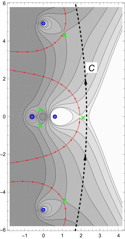
Figure 2: Contour plot of Re$[S(x)]$ as a function of complex variable $x$ for $n=5$, $t=4.5,\Gamma=1$, $\epsilon_{d}3$ and $\Delta=2$. The green crosses show roots of Eq. 42 and the points in the blue circles are poles of the function $Q_{n}(x)$. The thick dashed curve is the integration countour $C$. The red curves with arrows show the steepest descent path for the contour transformation.

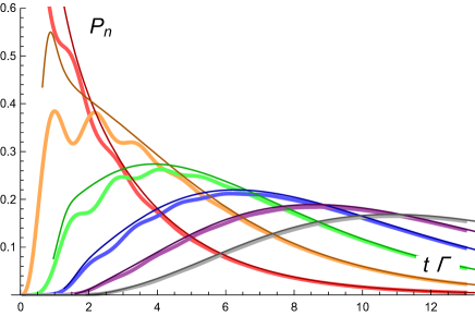
Figure 3: Plot of the probabilities $P_{n}$ in Eq. 39 as a function of $t$ for $\epsilon_{d}/\Gamma=3$ and $\Delta/\Gamma=2$. The red, brown, green, blue, purple and grey lines correspond to the parameter $n=$ 0, 1, 2, 3, 4, and 5. The thin curves of the same colors illustrate Eq. 40 for the same parameters $n$, $\epsilon_{d}/\Gamma$ and $\Delta/\Gamma$.

The asymptotic expression (44) is a Gaussian function of time that satisfies, in fact, the general relation

$$\int_{0}^{\infty}P_{n}(t)dt=Q_{n}(\Gamma)=I_{0}^{-1}\ ,$$ (46)

which follows from Eq. ( 35) as a direct consequence of $p_{4}(x,w)$ being linear in $w$ and $p_{4}(\Gamma,1)=0$. The integral in (46) gives us a visibility time frame for observation of the fixed number tunnelings.

V Current cumulants and transient extra charge

Next, we avail of the generating function ( 35) in the standard way to obtain the average moments of the charge distribution and its cumulants. The latter growing linearly with time are particular convenient to characterize the long time behavior of the charge distribution, while the formers describe the transient behavior of the charge distribution and, in particular, the oscillatory transient current epl .

The suitable $P(w,t)$ expression follows from calculation of the integral in Eq. (35) by closing the contour $C$ in the left half-plane and counting the residues of the four integrand poles defined by the roots $x_{l},\ l=-1\div 2$ of $p_{4}(x)$ in Eq. (36). which results in

$$P(t,w)=\sum\limits_{l=-1}^{2}q_{l}(w)\exp[(x_{l}(w)-\Gamma)t]\,.$$ (47)

Here the coefficients

$$q_{l}(w)=\frac{\Gamma\epsilon_{d}^{2}+\epsilon_{d}^{2}x_{l}+\Gamma x_{l}^{2}+4\Delta^{2}x_{l}+x_{l}^{3}}{2x_{l}\left(\epsilon_{d}^{2}-\Gamma^{2}+4\Delta^{2}\right)+4x_{l}^{3}-4\Gamma\Delta^{2}w}$$ (48)

do not depend on time and should meet the following conditions:

$$\partial_{w}^{n}\sum\limits_{l=-1}^{2}q_{l}(w)=0=\partial_{w}^{n}\sum\limits_{l=-1}^{2}q_{l}(w)x_{l}(w)|_{w=1}\,,\ n\geq 1\,.$$ (49)

The first of these restrictions stems from the normalization $P(w,0)=1$, while the second equation reflects that the process starts from the empty state of QD, since the moments of the transferred charge are given by $\left\langle N^{n}(t)\right\rangle=(w\partial_{w})^{n}P(t,w)$ at $w=1$. It also means that the sum on the right-hand side is a constant around $w=1$.

The long time behavior of the moments is determined by the term in Eq. (47) with the main root $x_{0}(w)$ exponent, where

$$x_{0}(1)=\Gamma\ \ \mbox{and}\ \ q_{0}(1)=1\,.$$ (50)

The other exponents in Eq. (47) contribute to the transient behavior of the transferred charge moments and specify, in particular, the transient current time dependence $\left\langle I(t)\right\rangle$. From calculation of the transient current in epl we conclude that $q_{l}(1)=0$, if $l\neq 0$, and

$$\left\langle I(t)\right\rangle=x_{0}^{\prime}(1)+\sum_{l\neq 0}q_{l}^{\prime}(1)(x_{l}(1)-\Gamma)\exp[(x_{l}(1)-\Gamma)t]$$ (51)

Although the prefactor $q_{0}(w)$ at the main exponent in Eq. (47) does not contribute to the transient current it contains information of the total charge accumulation. Indeed, integrating the right-hand side of Eq. (51) over time and using the relation (49) one finds the transient extra in the long time asymptotics of the average charge as follows

$$\delta\left\langle N(t)\right\rangle=\left\langle N(t)\right\rangle-tI_{0}\asymp q_{0}^{\prime}(1)\,,t\rightarrow\infty$$ (52)

Direct differentiation of Eq. (48) gives us the explicit expression for the average extra charge:

$$q_{0}^{\prime}(1)=\frac{\Delta^{2}(\epsilon_{d}^{2}-3\Gamma^{2})}{(\epsilon_{d}^{2}+\Gamma^{2}+2\Delta^{2})^{2}}\ ,$$ (53)

which is negative near the resonance and becomes positive if $\epsilon_{d}^{2}$ exceeds $3\Gamma^{2}$. As the integral of the function $\left\langle I(t)\right\rangle-I_{0}$ the average extra charge can be positive only if the transient current $\left\langle I(t)\right\rangle$ varies from $\left\langle I(0)\right\rangle=0$ to $\left\langle I(\infty)\right\rangle=I_{0}$ non-monotonically and grows bigger than $I_{0}$ at some times. This occurs in our system because of the oscillating behavior of the transient current as will be illustrated later on examples in Special regimes. Similarly can be found higher cumulants of the extra charge fluctuations, which we discuss below.

V.1 Zero frequency current cumulants

The leading asymptotics of $\ln P(w,t)$ at large $t$ and $w\approx 1$ is specified by the largest root of $p_{4}$ as

$$\ln P(t,w)\asymp t[x_{0}(w)-\Gamma]+\ln q_{0}(w).$$ (54)

Then $x_{0}(w)$ serves as the CGF and the reduced zero-frequency current correlator or cumulant of the $n$th order is $\left\langle\left\langle I^{n}\right\rangle\right\rangle=(w\partial_{w})^{n}x_{0}(w)$ at $w=1$.

Since the explicit analytic expression for the root is too cumbersome, we will calculate the cumulants $\langle\langle I^{n}\rangle\rangle$ through the root Taylor expansion around $w=1$ in the following form:

$$x_{0}(\,e^{i\chi})=\Gamma+\sum\limits_{n=1}\left\langle\left\langle I^{n}\right\rangle\right\rangle(i\chi)^{n}/n!\,.$$ (55)

Normalizing the results $F_{n}=\left\langle\left\langle I^{n}\right\rangle\right\rangle/I_{0}$ we find the Fano factor equal to:

$$F_{2}=1+\frac{2\Delta^{2}(\epsilon_{d}^{2}-3\Gamma^{2})}{(\epsilon_{d}^{2}+\Gamma^{2}+2\Delta^{2})^{2}}\$$ (56)

and its behavior is shown in Fig. (4).

This expression shows the clear border $\epsilon_{d}^{2}=3\Gamma^{2}$ between the sub-Poissonian current fluctuations near the resonance at $\epsilon_{d}=0$ and the super-Poissonian ones far from it. From comparison of Eqs. (53) and (56) we conclude that

$$F_{2}=1+2\delta\left\langle N(\infty)\right\rangle.$$ (57)

The reason for this seemingly accidental relation between the Fano factor and the average extra charge will be clarified below. The Fano factor $F_{2}$ reaches its minimum $F_{2}=0.25$ at $\epsilon_{d}=0$ and $\Delta=\Gamma/\sqrt{2}$ and it asymptotically approaches its maximum $F_{2}\rightarrow 1.25$ as $\epsilon_{d}=\sqrt{2}\Delta\rightarrow\infty$.

The third order normalized commulant called skewness is equal to

$$\!\!\!\!\!F_{3}=1+\frac{48\left(4\Gamma^{4}\Delta^{4}+4\Gamma^{2}\Delta^{6}+\Delta^{8}\right)}{\left(\Gamma^{2}+\epsilon_{d}^{2}+2\Delta^{2}\right){}^{4}}+$$ (58)

$$\!\!\!\!\!\frac{6\Delta^{2}\left(\epsilon_{d}^{4}-3\Gamma^{4}-22\Gamma^{2}\Delta^{2}-2\left(\Gamma^{2}-\Delta^{2}\right)\epsilon_{d}^{2}-4\Delta^{4}\right)}{\left(\Gamma^{2}+\epsilon_{d}^{2}+2\Delta^{2}\right){}^{3}}\ .$$

and depicted in Figs. (5,6). Among the special features of its behavior we observe a small parametric area, where the skewness is negative, and also appearance of a plateau in its parameter dependence at the degeneracy point $2\Delta=\Gamma,\epsilon_{d}=0$ characterized by the transition probabilities in Eq. (31).

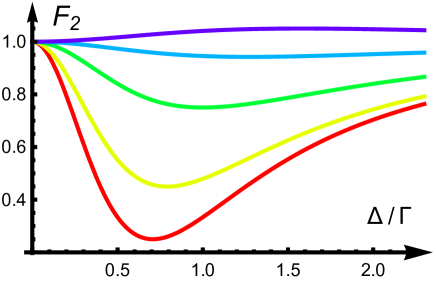
Figure 4: Plot of the Fano factor $F_{2}$ in Eq. 56 as a function of $\Delta/\Gamma$. The red, yellow, green, light blue and blue lines correspond to the parameter $\epsilon_{d}/\Gamma=$ 0, 0.5, 1, 1.5, and 2.

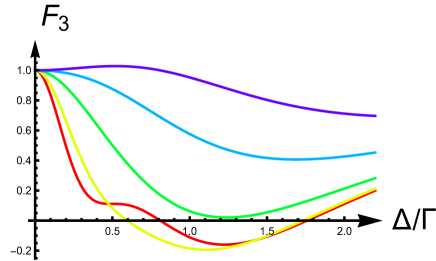
Figure 5: Plot of the skewness $F_{3}$ in Eq. 58 as a function of $\Delta/\Gamma$. The red, yellow, green, light blue and blue lines correspond to the parameter $\epsilon_{d}/\Gamma=$ 0, 0.5, 1, 1.5, and 2.

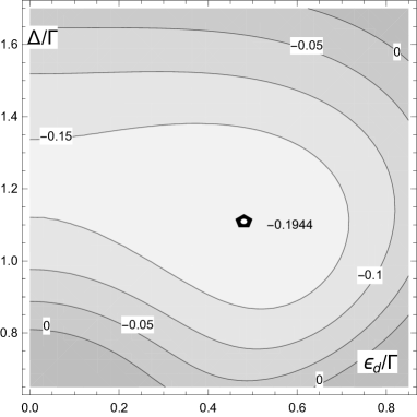
Figure 6: Plot of the area where the skewness $F_{3}$ in Eq. 58 is negative as a function of $\Delta/\Gamma$ and $\epsilon_{d}/\Gamma$. The black pentagon with white point indicates its absolute minimum.

V.2 Transient extra charge fluctuations and Fano factors

As follows from Eq. (54) the long time asymptotics of the cumulants of the transferred charge statistics:

$$\left\langle\left\langle N^{n}(t)\right\rangle\right\rangle\asymp tI_{0}F_{n}+(w\partial)^{n}\ln q_{0}(w)|_{w=1}.$$ (59)

contains besides the terms growing linearly in time and defined by the Fano factors $F_{n}$, the additional non-universal contributions due to the transient extra charge accumulation depending on the initial state of QD. The extra charge cumulants are defined by their CGF $\ln q_{0}(w)$ and could be formally considered as a result of an independent additional charge transfer process. This process, however, does not make a clear physical sense as the extra charge second order cumulant

$$\!\!\!\!\!\delta\left\langle\left\langle N^{2}\!\right\rangle\right\rangle=\frac{d[w(d\ln[q_{0}])}{dw^{2}}=\frac{I_{0}{}^{4}\left(\epsilon_{d}^{2}-3\Gamma^{2}\right)\left(\Gamma^{2}+\epsilon_{d}^{2}\right){}^{2}}{16\Gamma^{4}\Delta^{6}}$$

$$\!\!\!\!\!+\frac{I_{0}{}^{4}\left(25\Gamma^{4}-54\Gamma^{2}\epsilon_{d}^{2}+\epsilon_{d}^{4}\right)}{16\Gamma^{4}\Delta^{4}}-\frac{I_{0}{}^{4}\left(7\Gamma^{2}+3\epsilon_{d}^{2}\right)}{4\Gamma^{4}\Delta^{2}}$$ (60)

is not always non-negative.

The expression for the long time asymptotics of the transferred charge cumulants analogous to Eq. ( 59) can also be written for the steady evolution process starting in the stationary QD state. However, in this case there is no additional average charge accumulation $\left\langle N(t)\right\rangle_{st}=I_{0}t$ and hence $q_{st,0}^{\prime}(1)=0$. Making use of the general relation between the generating functions for both processes we substitute their asymptotics (54) into Eq. ( 15) and find that

$$x_{0}(w)-\Gamma=(w-1)I_{0}q_{0}(w)/q_{st,0}(w).$$ (61)

Taking the second derivative of this equation with respect to $i\chi$ at $w=\exp(i\chi)=1$ we come to the relation $F_{2}=1+2q_{0}^{\prime}(1)$ derived earlier in (57) between the Fano factor and the extra transient average charge $\delta\left\langle N(\infty)\right\rangle$ as defined in Eq. (52). This relation explains, in particular, that the super Poissonian current fluctuations in this system occurs due to an excess of the average transient charge accumulated in the tunneling process initiated in the empty state of QD, contrary to the more common sub Poissonian current shot noise, which happens if there is a deficit of this average charge. Moreover, since the excessive average charge needs a non-monotonous time dependence of the transient current, the emergence of the super Poissonian noise is a finger-print of the qubit coherent dynamics in the system and an oscillating behavior of the transient current.

Taking the third derivative of Eq. ( 61) we can write the third order Fano factor in the following form

$$F_{3}=1+\frac{3}{4}[F_{2}^{2}-1]+3[\delta\left\langle\left\langle\!N^{2}\!\right\rangle\right\rangle-\!\delta\left\langle\left\langle\!N^{2}\!\right\rangle\right\rangle_{st}]\ ,$$ (62)

which relates the skewness to the difference in the transient extra charge fluctuations in the two processes. Although the second term on the right-hand side in (62) is negative for the sub-Poissonian noise, the whole skewness also becomes negative only when the second order cumulant defined by $\delta\left\langle\left\langle\!N^{2}\!\right\rangle\right\rangle_{st}=\left\langle\left\langle\!N^{2}(t)\!\right\rangle\right\rangle_{st}-I_{0}F_{2}t$ at large $t$ and characterizing the extra fluctuations of the charge accumulated in the steady evolution process is much bigger than the corresponding cumulant $\delta\left\langle\left\langle\!N^{2}\!\right\rangle\right\rangle=\left\langle\left\langle\!N^{2}(t)\!\right\rangle\right\rangle-I_{0}F_{2}t$ at large $t$ of the extra charge fluctuations in the case of the evolution process starting from the empty QD. The area where $F_{3}<0$ is shown on Fig.6.

V.3 Special regimes

From the $p_{4}(x)$ expression in the integrand denominator in Eq. (35) we find the linear in $w$ dependence of the roots as $x_{0,2}=\pm\mu+x_{0}^{\prime}(0)w$ and $x_{\pm 1}(w)=\pm i\omega_{e}-x_{0}^{\prime}(0)w$, where

$$x_{0}^{\prime}(0)=\frac{2\Delta^{2}\Gamma}{\omega_{e}^{2}+\mu^{2}}\$$ (63)

is well defined except for at the degeneracy point.

The linear root approximations can be extended up to $w=1$ if $x_{0}^{\prime}(0)\ll|\mu|,\omega_{e}$. This limits their applicability to $\Gamma^{2}+\epsilon_{d}^{2}\gg 4\Delta^{2}$, where $x_{0}^{\prime}(0)=2\Delta^{2}\Gamma/(\Gamma^{2}+\epsilon_{d}^{2})\approx I_{0}$. Making use of these root approximations in calculation of the Laplace transformation in Eq. (35) we find

$$\!\!\!\!\!P(t,w)=\left[1+\frac{\Delta^{2}(w-1)\left(\epsilon_{d}^{2}-3\Gamma^{2}\right)}{\left(\Gamma^{2}+\epsilon_{d}^{2}\right){}^{2}}\right]e^{tI_{0}(w-1)}$$ (64)

$$\!\!\!\!+\frac{2\Gamma^{2}\Delta^{2}(w-1)e^{-(I_{0}w+\Gamma)t}}{\left(\Gamma^{2}+\epsilon_{d}^{2}\right){}^{2}}\sum_{\pm}\left[1\pm i\frac{\epsilon_{d}}{\Gamma}\right]e^{\pm it\epsilon_{d}(1+I_{0}/\Gamma)}$$

$$\!\!\!\!-\frac{\Delta^{2}(w-1)e^{t\left(I_{0}(w+1)-2\Gamma\right)}}{\Gamma^{2}+\epsilon_{d}^{2}}+O(I_{0}^{2}/\Gamma^{2})\,.$$

The main exponent in Eq.( 64) coincides with the Poissonian defined by the single long living mode of the probability $P_{0}(t)$ in (33). The prefacot at the main exponent shows that due to the charge accumulated in the transient regime of $\Gamma t<1$ this Poissonian eventually acquires an excessive charge of one binomial attempt in the long time limit for $\epsilon_{d}^{2}>3\Gamma^{2}$ and the lack of it, otherwise. The first regime is the super-Poissonian in agreement with Eq. (56) and the other is the sub-Poissonian. To clarify the physical mechanism of transition between these two regimes we exploit the generating function asymptotics (64 ) to calculate the deviation of the transient current from its long-time stationary limit

$$\left\langle\delta I(t)\right\rangle=I_{0}[e^{-2\Gamma t}-2\cos(\epsilon_{d}t)e^{-\Gamma t}+O(I_{0}/\Gamma)]\ ,$$ (65)

which shows how increase of the frequency of the current oscillations in comparison to the decay rate diminishes contribution of the oscillating term on the right-hand side of (65 ) into the extra charge accumulation and makes the average extra charge excessive.

In the opposite regime of large $\Delta$, where $\Gamma^{2}+\epsilon^{2}_{d}\ll 4\Delta^{2}$, the roots dependence on $w$h starting from their initial values in Eq. (34) can be found with increase of $w$ in $p_{4}(x)$ in the following way. $x_{\pm}(w)$ due to their large imaginary parts undergo just the linear shift as $x_{\pm}(w)=\pm i\omega_{e}-\Gamma w/2$. Meanwhile the $x_{0,2}$ dependences are essentially non-linear and at $w\approx 1$ are given by

$$x_{2}=-\frac{\Gamma\epsilon_{d}^{2}}{4\Delta^{2}w}\,,\ x_{0}=\frac{\Gamma w}{4\Delta^{2}}(4\Delta^{2}-\epsilon_{d}^{2}+(1-w^{2})\Gamma^{2})-x_{2}\,.$$ (66)

Making use of Eq. (48) with these roots approximation under condition $\epsilon_{d}^{2}\gg\Gamma^{2}$ we find the asymptotics of the generating function in this super Poissonian regime as

$$\!\!\!\!\!P(t,w)=-\frac{\epsilon_{d}^{2}(w-1)e^{-\Gamma(1+\frac{\epsilon_{d}^{2}}{4\Delta^{2}w})t}}{4w^{2}\Delta^{2}}+$$ (67)

$$\!\!\!\!\left(1+\frac{\epsilon_{d}^{2}(w-1)}{4\Delta^{2}w^{2}}\right)e^{\Gamma\left(1-\frac{\epsilon_{d}^{2}}{4\Delta^{2}}\right)(w-1)t+\frac{\Gamma\epsilon_{d}^{2}}{4\Delta^{2}}\left(\frac{1}{w}-1\right)t}-$$

$$\!\!\!\!\!\frac{4\Gamma\Delta^{2}(w-1)\sin\left(t\sqrt{\epsilon_{d}^{2}+4\Delta^{2}}\right)e^{-\Gamma\left(\frac{2\Delta^{2}w}{\epsilon_{d}^{2}+4\Delta^{2}}+1\right)t}}{\left(\epsilon_{d}^{2}+4\Delta^{2}\right){}^{3/2}}$$

The long-time behavior of the generating function specified by the leading exponent in (67 ) presents the total tunneling process as a combination of the two independent processes. Those are the main Poissonian of electrons tunneling characterized by the tunneling rate $\Gamma\left[1-\epsilon_{d}^{2}/(4\Delta^{2})\right]$ and its weak counterpart Poissonian of holes tunneling with the small rate $\Gamma\epsilon_{d}^{2}/(4\Delta^{2})$, which develops as the level position deviates from the resonance. This makes the total process super Poissonian since the total average current comes as difference of the tunneling rates, while the total noise is their sum.

The deviation of the transient current from its long-time stationary limit follows from (67) as

$$\left\langle\delta I(t)\right\rangle=\frac{\Gamma\epsilon_{d}^{2}e^{-\Gamma t(1+\frac{\epsilon_{d}^{2}}{4\Delta^{2}})}}{4\Delta^{2}}-\frac{4\Gamma\Delta^{2}e^{-\Gamma t(\frac{3}{2}-\frac{\epsilon_{d}^{2}}{8\Delta^{2}}})}{\omega_{e}^{2}}\cos(\omega_{e}t)\ .$$ (68)

Its integration over time shows that high frequency oscillations of the second term make the first term contribution into the average extra charge prevail with the result: $\left\langle\delta N(\infty)\right\rangle=(\epsilon_{d}^{2}-3\Gamma^{2})/(4\Delta^{2})$.

At the resonance we find from Eq. (36 ) that $p_{4}(x,w)=xp_{3}(x)$, where

$$p_{3}(x)=x^{3}+(4\Delta^{2}-\Gamma^{2})x-4\Delta^{2}\Gamma w$$ (69)

and besides the root $x_{2}=0$ the three other roots read Jacobson as follows

$$x_{l}=\Gamma\sum_{\pm}e^{\pm\frac{2\pi il}{3}}\left(2\Delta_{\Gamma}^{2}w\pm\sqrt{4\Delta_{\Gamma}^{4}w^{2}+[(4\Delta_{\Gamma}^{2}-1)/3]^{3}}\right)^{\frac{1}{3}}$$ (70)

where $\Delta_{\Gamma}=\Delta/\Gamma$. The cumulant generating function is

$$\ln P(t,w)\asymp t(x_{0}-\Gamma)+\ln\frac{4\Gamma^{2}\Delta_{\Gamma}^{2}+\Gamma x_{0}+x_{0}^{2}}{\Gamma^{2}\left(4\Delta_{\Gamma}^{2}-1\right)+3x_{0}^{2}}$$ (71)

In both limits $\Delta_{\Gamma}\ll 1$ and $\Delta_{\Gamma}\gg 1$ it takes the Poissonian form $\ln P(t,w)/t\asymp I_{0}[w-1]$ with the average current $I_{0}=2\Delta^{2}/\Gamma$ and $I_{0}=\Gamma$, respectively.

At the degeneracy point of the qubit modes when $2\Delta=\Gamma,\epsilon_{d}=0$, the four roots of $p_{4}(x,w)$ follow from Eq. (69) as $x_{l}=e^{i2\pi l/3}\Gamma w^{1/3},x_{2}=0$. With $g_{E}(x)$ defined in Eq. (29) the generating function comes up after taking the Laplace transformation integral in the form:

$$P(t,w)\!=\!\!\!\sum\limits_{l=-1}^{1}\frac{(w+e^{i\frac{2\pi}{3}l}w^{\frac{1}{3}}+e^{i\frac{4\pi}{3}l}w^{\frac{2}{3}})e^{\Gamma t(e^{i\frac{2\pi}{3}l}w^{\frac{1}{3}}-1)}}{3w}.$$ (72)

For $w$ in the sector around the real positive axis this function converges at large time to the Poissonian of the fractional charge $1/3$ modified by an independent tunneling of one and two fractional holes, which leads to the $1/3$ deficit of the average Poissonian charge. Since all zero-frequency current cumulants are defined by the generating function asymptotics at $w=1$ and large $t$ (see below) they all coincides with the Poissonian cumulants equal $\Gamma/3^{n}$ in the $n$th order as if we observe the fractional charge tunneling process.

However there is no fractional charge tunneling in the complete generating function in Eq. (72) because the $2\pi$ periodicity with respect to the $w$ phase guaranies that $P(t,w)$ remains the integer function of $w$. Calculating its coefficients as

$$P_{n}(t)\!=\left(\frac{(\Gamma t)^{3n}}{3n!}+\frac{(\Gamma t)^{3n+1}}{(3n+1)!}+\frac{(\Gamma t)^{3n+2}}{(3n+2)!}\right)e^{-\Gamma t}$$ (73)

we find the explicit expansion of the complete generating function in the following form:

$$P(t,w)\!=e^{-\Gamma t}\sum\limits_{m=0}^{\infty}\frac{(\Gamma t)^{m}}{m!}w^{[m/3]}\,,$$ (74)

where $[x]$ denotes the integer part of $x$ or its antie function. It is a reduced Poissonian distribution due to unsuccessful tunneling attempts by the fractional charges.

VI Conclusion

Tunneling of spinless electrons through an interacting resonant level of a QD into an empty collector has been studied in the especially simple, but realistic system, in which all sudden variations in charge of the QD are effectively screened by a single tunneling channel of the emitter. This system has been described epl with an exactly solvable model of a dissipative two-level system called qubit. Its matrix element $\Delta$ of the coupling between the two-level states is equal to the bare emitter tunneling rate $\Gamma_{e}$ renormalized by the large factor $\sqrt{D/(\pi\Gamma_{e})},$ whereas the damping parameter $\Gamma$ coincides with the tunneling rate into the collector.

The exact solution to this model was earlier used to demonstrate that the coherent qubit dynamics expected in the FES regime should manifest themselves in an oscillating behavior epl of the average collector transient current in the wide range of the model parameters and also through the resonant features of the a.c. response prb , though the experimental observation of these manifestations could be a difficult experimental task. Therefore, in this work we have studied more relevant electron transport characteristics to the modern experiments including Fano factor of the second 8 and third (skewness) orders shovkun ; third . In particular, we have clarified a possible mechanism leading to appearance of the sub-Poisson and super Poisson shot noise of the tunneling current as it has been observed in the recent experiments noise ; noise2 in the FES regime.

In this work we have used the method of full counting statistics to calculate the generating function of the distribution of charge transferred in process of the empty QD evolution, which is governed by the generalized Lindblat equation. This equation describes the whole process as a succession of time periods of the non-Hermitian Hamiltonian qubit evolution randomly interrupted by the electron tunneling jumps from the occupied QD into the empty collector. The qubit density matrix evolution during each of these periods has been described as a four mode process, two modes of which are oscillating with opposite frequencies and the same damping rate $\Gamma$ about everywhere except for at the exact resonance $\epsilon_{d}=0$ and $\Gamma>2\Delta$ . As a result the time dependent probabilities $P_{n}(t)$ to have a certain number $n$ of electrons tunneled into the collector, which are determined by the matrix element of the density matrix undergoing the non-Hermitian Hamiltonian evolution, are also oscillating except for the same infinitely narrow parametric area. These oscillations are better visible at small time and therefore for $P_{n}(t)$ with small number $n$, since the slowest damping mode is not oscillating. Note, however, that the frequency of these oscillations is different from the one of the transient current: Both are the transformations of the two-level energy split of the isolated qubit by the dissipation, though the first one accounts for expectation for the electron tunneling into the collector, but without its real occurrence, meanwhile the second one is due to both effects.

The four modes of the Hamiltonian evolution of the qubit density matrix lead to a general representation of the generating function as a sum of the four exponents with linear in time arguments, which are multiplied by the exponent prefactors. The long time behavior of this function with the counting parameter $w\approx 1$ is determined by the leading exponent term. Its logarithm gives us the long time asymptotics of the CGF consisting of the two parts, which describe two independent contributions into the transferred charge fluctuations. The part linearly growing in time defines the zero-frequency current cumulants and has been used to calculate the Fano factor and the skewness. It does not depend on the initial state of the QD and hence on the transient evolution behavior. Contrary, the other part given by the prefactor logarithm depends on the QD initial state and has been used as the CGF of the transient extra charge fluctuations.

Our calculation of the Fano factor has shown emergence of the sub Poissonian behavior of the current fluctuations near the resonance which changes into the super Poissonian as the level energy moves out of the resonance and $\epsilon_{d}^{2}>3\Gamma^{2}$. On the other hand, from our consideration of the extra charge CGFs we have found the simple linear relation between the Fano factor and the average transient extra charge accumulated during the empty QD evolution. It explains that the sub and super Poissonian steady current statistics correspond to the transient accumulation of the negative and positive average extra charge, respectively. Moreover, the positive average extra charge can be accumulated only if the transient current is non-monotonous in time. Therefore, emergence of the super Poissonian steady current fluctuations signals an oscillating behavior of the transient current and the qubit coherent dynamics according to this model of the FES.

We have also calculated the skewness and found that it changes its sign and becomes negative in the small area near the resonance, where $|\epsilon_{d}|<\Gamma$ and $0.6\lesssim\Delta/\Gamma\lesssim 1.8$. We have understood this behavior through comparison of the extra charge CGFs for the QD evolutions starting from its empty and stationary states, which has related the skewness to the difference between the two extra charge cumulants of the second order characterizing difference between the total charge noise in these two processes. This relation has shown that the skewness becomes negative in the sub Poissonian regime, if the total charge noise developed in the stationary state evolution is much bigger than the one in the evolution of the empty state.

These relations between the steady current fluctuations and the extra charge accumulation have been illustrated with particular examples of the generating functions in the special regimes. The two generating functions have been calculated asymptotically in the regimes when amplitude of the qubit two-level coupling is much smaller than the collector tunneling rate or the absolute value of the QD level energy and in the opposite limit when the amplitude is much larger than both of them. Accumulation of the extra charge in these regimes is illustrated with the corresponding transient current behavior.

We have also calculated the generating function at the special point $\Gamma=2\Delta$ at the resonance, when the two qubit levels energies including their imaginary parts are equal. We find that in this special case it takes the $1/3$ fractional Poissonian form, where all probabilities of tunneling of the fractional charges mean tunneling of the charges integer parts. The large time limit of this function, nontheless, coincides with the true $1/3$ fractional Poisson. This example underlines that observation of the fractional charge in the Poissonian shot noise is necessary, but not sufficient to prove its real tunneling.

We have performed our calculations in dimensionless units with $\hbar=1$ and $e=1$. In order to return to the SI units the current $I_{0}$ should also include the dimensional factor $e^{2}/\hbar\approx 2.43\cdot 10^{-4}$S, if $\Gamma,$ $\Delta,$ and $\epsilon_{d}$ are measured in volts. In the experiments lar ; lar1 the collector tunneling rate is $\Gamma\approx 0.1meV$ and the coupling parameter $\Delta\approx 0.016meV$. To observe the special regime of Eqs. (31,74) one can increase the collector barrier width to obtain a heterostructure with $\Delta=0.016meV$ and $\Gamma=2\Delta\approx 0.032meV$. Its stationary current at the resonance is $I_{0}=2.6\,nA$ and the zero frequency spectral density of the current noise measured in experiments as $S_{0}=2|e|I_{0}F_{2}$ with the above dimentional $I_{0}$ and $F_{2}$ from Eq. (56 ) is $S_{0}\approx 2.76\cdot 10^{-28}A^{2}/Hz$. With increase of $|\epsilon_{d}|$ the current $I_{0}$ is decreasing, whereas $S_{0}$ grows up to its maximum $S_{0}\approx 4.2\cdot 10^{-28}A^{2}/Hz$ at $|\epsilon_{d}|\approx 0.027meV$. At larger $|\epsilon_{d}|$ the current shot noise becomes super Poissonian with its zero frequency spectral density approaching $S_{0}\approx 2.5|e|I_{0}$. According to Ref. epl2 the finite frequency spectral density $S_{\omega}$ varies less then 20% if $\omega<\Gamma/(2\hbar)$. Since the frequency corresponding to the above value of $\Gamma$ is $\omega_{\Gamma}\sim 5\cdot 10^{10}s^{-1}$, we can consider the frequency $\omega$ low enough to evaluate $S_{0}$, if $\omega/(2\pi)$ is below $4\,GHz.$

- (1) G. D. Mahan, Phys. Rev. 163, 612 (1967).
- (2) P. Nozieres and C. T. de Dominicis, Phys. Rev. 178, 1097 (1969).
- (3) P. H. Citrin, Phys. Rev. B 8, 5545 (1973).
- (4) P. H. Citrin, G. K. Wertheim, and Y. Baer, Phys. Rev. B 16, 4256 (1977).
- (5) K. A. Matveev and A. I. Larkin, Phys. Rev. B 46, 15337 (1992).
- (6) A. K. Geim, P. C. Main, N. La Scala Jr., L. Eaves, T. J. Foster, P. H. Beton, J. W. Sakai, F. W. Sheard, M. Henini., G. Hill and M. A. Pate, Phys. Rev. Lett. 72, 2061 (1994)
- (7) I. Hapke-Wurst, U. Zeitler, H. Frahm, A. G. M. Jansen, R. J. Haug, and K. Pierz, Phys. Rev. B 62, 12621 (2000).
- (8) H. Frahm, C. von Zobeltitz, N. Maire, and R. J. Haug, Phys. Rev. B 74, 035329 (2006).
- (9) M. Ruth, T. Slobodskyy, C. Gould, G. Schmidt, and L. W. Molenkamp, Applied Physics Letters 93, 182104 (2008).
- (10) N. Maire, F. Hohls, T. Lüdtke, K. Pierz, and R. J. Haug, Phys. Rev. B 75, 233304 (2007).
- (11) I.A. Larkin, E.E. Vdovin, Yu.N. Khanin, S. Ujevic and M. Henini, Phys. Scripta, 82, 038106, (2010).
- (12) V.V. Ponomarenko and I. A. Larkin, EPL 113, 67004 (2016).
- (13) A. J. Leggett et al., Rev. Mod. Phys. 59, 1 (1987).
- (14) O. Katsuba and H. Schoeller, Phys. Rev. B 87, 201402(R) (2013).
- (15) N. Ubbelohde et al., Sci. Rep. 2, 374 (2012).
- (16) J.K. Kühne and R.J. Haug, Phys. Status Solidi B, 256, 1800510, (2019).
- (17) K. Roszak and T. Novotný, Phys. Scr. T151 014053 (2012).
- (18) Yu. Bomze, G. Gershon, D. Shovkun, L. S. Levitov, M. Reznikov, Phys. Rev. Lett. 95, 176601 (2005)
- (19) Tero T. Heikkilä and Teemu Ojanen; Phys. Rev. B 75, 035335, (2007).
- (20) V.V. Ponomarenko,and I.A. Larkin, Phys. Rev. B 95, 205416 (2017).
- (21) L. S. Levitov, H.-W. Lee, G. B. Lesovik, J. Math. Phys. 37, 4845 (1996); L.S Levitov and M. Reznikov, Phys. Rev. B 70, 115305 (2004).
- (22) D.A. Bagrets and Yu.V. Nazarov, Phys. Rev. B 67, 085316 (2003).
- (23) K. Schotte and U. Schotte, Phys. Rev. 182, 479 (1969).
- (24) J. König, J. Schmid, H. Schoeller, and G. Schön, Phys. Rev. B 54, 16820 (1996).
- (25) H.T. Imam, V.V. Ponomarenko, and D.V. Averin, Phys. Rev. B 50, 18288 (1994).
- (26) V.V. Ponomarenko and I. A. Larkin, EPL 125, 67004 (2019).
- (27) C. Timm, Phys. Rev. B, 77, 195416, (2008)
- (28) N. Jacobson, Basic algebra 1 (2nd ed.), Dover, (2009), ISBN 978-0-486-47189-1
- (29) I.A. Larkin, Yu.N. Khanin, E.E. Vdovin, S. Ujevic and M. Henini, J. Phys.: Conf. Ser. 456, 012024, ( 2013).
- (30) M V Fedoryuk, (2001), ”Saddle point method”, in Hazewinkel, Michiel, Encyclopedia of Mathematics, Springer Science Business Media, B.V. Kluwer Academic Publishers.
- (31) Seshadri, V. (1997). ”Halphen’s laws”. In Kotz, S.; Read, C. B.; Banks, D. L. Encyclopedia of Statistical Sciences, Update Volume 1. New York: Wiley. p. 302.