Stabilization of Filament Production Rate for Screw Extrusion-Based Polymer 3D-Printing

Abstract

Polymer 3D-printing has been commercialized rapidly during recent years, however, there remains a matter of improving the manufacturing speed. Screw extrusion has a strong potential to fasten the process through simultaneous operation of the filament production and the deposition. This paper develops a control algorithm for screw extrusion-based 3D printing of thermoplastic materials through an observer-based output feedback design. We consider the thermodynamic model describing the time evolution of the temperature profile of an extruded polymer by means of a partial differential equation (PDE) defined on the time-varying domain. The time evolution of the spatial domain is governed by an ordinary differential equation (ODE) that reflects the dynamics of the position of the phase change interface between polymer granules and molten polymer deposited as a molten filament. Steady-state profile of the distributed temperature along the extruder is obtained when the desired setpoint for the interface position is prescribed. To enhance the feasibility of our previous design, we develop a PDE observer to estimate the temperature profile via measured values of surface temperature and the interface position. An output feedback control law considering a cooling mechanism at the boundary inlet as an actuator is proposed. In extruders the control of raw material temperature is commonly achieved using preconditioners as part of the inlet feeding mechanism. For some given screw speeds that correspond to slow and fast operating modes, numerical simulations are conducted to prove the performance of the proposed controller. The convergence of the interface position to the desired setpoint is achieved under physically reasonable temperature profiles.

1 Introduction

On the verge of new manufacturing techniques, additive manufacturing stands out as versatile tool for high flexibility and fast adaptability in production. It is applicable in a variety of producing industries, ranging from tissue engineering [26], thermoplastics [31], metal [24] and ceramic [29] fabrication. One of the most popular types of 3D printing is Fused Deposition Modeling (FDM) [27], which uses filaments as raw material, that have to be precisely manufactured to achieve a good final product quality [1].

From the polymer processing and extrusion cooking industry, screw extruders are well-known devices. Results stated in [28, 30, 23, 25] give an in-depth description of screw geometrics, extruder setups and describe the dynamics of extrusion process consisting of a conveying zone, a melting zone, and a mixing zone. A mathematical description of such a model is derived by mass, momentum and energy balances and appears as coupled transport equations coupled through a moving interface. This model is used in [25] to describe an extrusion cooking process. The boundary control of a similar model is achieved in [5, 6] under the assumption of constant viscosity.

More recent contributions considered screw extrusion as a useful technology for 3D printing application [31, 7, 4] allowing to manufacture a wider variety of materials than FDM, while using polymer granules as raw material [31]. In [4], a time-delay control was developed on a model consisting of two phases similarly to [25]. In both cases, stabilization of the moving interface separating a conveying and a melting zone is achieved with a fast convergence rate. Another approach which enables to control screw extruders in 3D printing is proposed in [7], where an energy-based model is established, simplifying the implementation of the control law and circumventing difficulties with state measurement. In other words, the control of the outflow rate at the nozzle only relies on the measurement of the heater current and the screw speed.

In the screw extrusion process, solid material is convected from the feed to the nozzle located at the end of a heating chamber. The solid raw material is melted and mixed before being expelled through the nozzle as a thin filament. For these process, the thermal behavior is an important factor which characterize final product quality. In fact, heat is supplied into the system by the heaters surrounding the extruder’s barrel on the one hand and by the viscous heat generation due to a shearing effect [25] on the other hand. The process of the phase transition from solid to liquid polymer can be described as a Stefan problem [9]. In this context, the dynamics of the solid-liquid phase interface is derived from the energy conservation in which the latent heat required for melting is driven by the internal heat of the liquid phase, resulting in the interface velocity to be proportional to the temperature gradients of the adjacent phase. For instance, in [8], the Stefan problem for a polymer crystallization process is described, and the analytical crystallization time is derived.

From a control perspective, the boundary stabilization of the interface position for the one-phase Stefan problem was recently developed in [10]–[19] based on the ”backstepping method” [21, 22]. More precisely, in [12], the observer-based output feedback control was designed via a nonlinear backstepping transformation and the exponentially stabilization of the closed-loop system was proved without imposing any a priori assumption. Similarly, in [13] the full-state feedback control design for the one-phase Stefan problem with flowing liquid was achieved enabling to exponentially stabilize the system to a constant steady-state. The application of the backstepping method for Stefan problem to the aforementioned 3D-printing process was covered in [17] by developing the thermodynamic model including the effects of screw speed and the barrel temperature, and designing the full-state feedback control law to stabilize the ratio between the polymer granules and melt polymer.

This paper extends the results in [17] by:

• $\bullet$ developing a PDE observer to estimate the temperature profile of the solid polymer granules with utilizing available measurements,

• $\bullet$ designing the associated observer-based output feedback control law and proving the stability of closed-loop system,

• $\bullet$ and verifying the performance of the designed observer and output feedback control law in numerical simulation.

First, the thermodynamic model of the polymer granules and melt polymer in screw extrusion is described, and the steady-state temperature profiles given by a prescribed setpoint of the interface position are analytically solved as in [17]. Second, a PDE observer is constructed as a copy of the plant plus the measurement error of the surface temperature multiplied by a constant observer gain. The designed observer is shown to be exponentially convergent to the granular pellets’ temperature profile along the heating chamber of the extruder. Third, using the designed observer, the output feedback control law for the boundary heat flux to stabilize the interface position at the desired setpoint is derived based on a similar manner to the full-state feedback design in [17], and the stability of the closed-loop system is proved under some realistic assumptions. Finally, simulation results are provided to illustrate the desired performance of the designed observer and the output feedback control design for some given screw speeds that correspond to slow and fast operating extrusion process.

This paper is organized as follows. The thermodynamic model of the screw extruder is developed in Section 2, and the steady-state analysis is provided in Section 3. The observer design is presented in Section 4, and the associated output feedback control design is derived in Section 5. The stability proof of the entire closed-loop system for a specific setup is established in Section 6. Simulation results are presented in order to analyze the controller’s performance in Section 7. We complete the paper in Section 8 with concluding remarks.

2 Thermodynamic Model of Screw Extruder

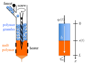
Figure 1: Schematic of screw extruder for original description (left) and model description (right).

We focus on the thermodynamic model of the screw extrusion process in one-dimensional coordinate along the vertical axis, motivated by [30] which developed a thermodynamic phase change model for polymer processing. The model provides the time evolution of the temperature profile of the extruded material and the interface position between the feeded polymer granules and the molten polymer. The granular pellets are conveyed by the screw rotation at a given speed $b$ along the vertical axis while the barrel temperature is uniformly maintained at $T_{{\rm b}}$. Defining $T_{{\rm s}}(x,t)$ and $T_{{\rm l}}(x,t)$ as the temperature profiles of solid phase (polymer granules) over the spatial domain $x\in(0,s(t))$ and liquid phase (molten polymer) over the spatial domain $x\in(s(t),L)$, respectively, the following thermodynamical model

$$\frac{\partial T_{{\rm s}}}{\partial t}(x,t)= \alpha_{{\rm s}}\frac{\partial^{2}T_{{\rm s}}}{\partial x^{2}}(x,t)-b\frac{\partial T_{{\rm s}}}{\partial x}(x,t)$$

$$+h_{{\rm s}}\left(T_{{\rm b}}-T_{{\rm s}}(x,t)\right),\textrm{for}\quad 0<x<s(t),$$ (1)

$$\frac{\partial T_{{\rm l}}}{\partial t}(x,t)= \alpha_{{\rm l}}\frac{\partial^{2}T_{{\rm l}}}{\partial x^{2}}(x,t)-b\frac{\partial T_{{\rm l}}}{\partial x}(x,t)$$

$$+h_{{\rm l}}\left(T_{{\rm b}}-T_{{\rm l}}(x,t)\right),\textrm{for}\quad s(t)<x<L$$ (2)

is derived from the energy conservation and heat conduction laws. In this paper, we consider the temperature distribution in the liquid to be static as stated in (11) and in Assumption 3 (see Section 5.1). Here, $\alpha_{i}=\frac{k_{i}}{\rho_{i}c_{i}}$ and $h_{i}=\frac{\bar{h}_{i}}{\rho_{i}c_{i}}$, where $\rho_{i}$, $c_{i}$, $k_{i}$, and $\bar{h}_{i}$ for $i\in\{s,l\}$ are the density, the heat capacity, the thermal conductivity, and the heat transfer coefficient, respectively and the subscripts $s$ and $l$ are associated to the solid or liquid phase, respectively. Referring to [32] which introduces a model of spatially averaged temperature for screw extrusion, we incorporate the convective heat transfer through the barrel temperature in (2) (2). The boundary conditions at $x=0$ and $x=L$ follow the heat conduction law, and the temperature at the interface $x=s(t)$ is maintained at the melting point $T_{{\rm m}}$, described as

$$\frac{\partial T_{{\rm s}}}{\partial x}(0,t)=-\frac{q_{{\rm f}}(t)}{k_{{\rm s}}},\quad T_{{\rm s}}(s(t),t)=T_{{\rm m}},$$ (3)

$$\frac{\partial T_{{\rm l}}}{\partial x}(L,t)=\frac{q_{{\rm m}}^{*}}{k_{{\rm l}}},\quad T_{{\rm l}}(s(t),t)=T_{{\rm m}},$$ (4)

where $q_{{\rm f}}(t)<0$ is a freezing controller at the inlet and $q_{{\rm m}}^{*}>0$ is a heat flux at the nozzle which is assumed to be constant in time. The interface dynamics is derived by the energy balance at the interface as

$$\rho_{s}\Delta H\dot{s}(t)=k_{{\rm s}}\frac{\partial T_{{\rm s}}}{\partial x}(s(t),t)-k_{{\rm l}}\frac{\partial T_{{\rm l}}}{\partial x}(s(t),t).$$ (5)

The equations (2)-(5) are the solid-liquid phase change model known as ”two-phase Stefan problem”. Such a phase change model was developed for polymer processing

Remark 1

In this paper, we assume the pressure in the chamber to be static and the melting temperature is constant to avoid supercooling. Then, to keep the physical state of each phase, the following conditions must hold:

$$T_{{\rm s}}(x,t)\leq T_{{\rm m}},\quad\forall x\in(0,s(t)),\quad\forall t>0,$$ (6)

$$T_{{\rm l}}(x,t)\geq T_{{\rm m}},\quad\forall x\in(s(t),L),\quad\forall t>0,$$ (7)

which represent the model validity conditions.

Remark 2

We assume the existence of a heating/cooling system that maintains the pellets at a controlled temperature as stated in (3), which describes the heat flux control at the inlet. Extruders can be equipped with raw material preconditioners as intermediate unit operators, which for instance help to pre-heat ingredients before they enter the extruder chamber by adding steam. The prconditioners are usually located between the inlet and the extruder chamber and a continuous flow of material from the feeder to the preconditioner is maintained [2, 3].

3 Steady-state and analysis

To ensure a continuous extrusion process, the control of the quantity of molten polymer that remains in the extruder chamber at any given time is crucial. By definition, the volume of fully melted material contained in the chamber is directly related to the position of the solid-liquid interface that needs to be controlled, consequently. Physically, any given position of the interface along the spatial domain correspond to a melt temperature profile along the extruder.

3.1 Steady-state solution

An analytical solution of the steady-state temperature profile denoted as $\left(T_{{\rm s},{\rm eq}}(x),T_{{\rm l},{\rm eq}}(x)\right)$ for any given setpoint value of the interface position defined as $s_{{\rm r}}$, can be computed by setting the time derivative of the system (2)-(5) to zero. Hence, from (2) and (2) the following set of ordinary differential equations in space are obtained

$$\begin{cases}0=&\alpha_{{\rm s}}T_{{\rm s},{\rm eq}}^{\prime\prime}(x)-bT_{{\rm s},{\rm eq}}^{\prime}(x)+h_{{\rm s}}\left(T_{{\rm b}}-T_{{\rm s},{\rm eq}}(x)\right),\\ 0=&\alpha_{{\rm l}}T_{{\rm l},{\rm eq}}^{\prime\prime}(x)-bT_{{\rm l},{\rm eq}}^{\prime}(x)+h_{{\rm l}}\left(T_{{\rm b}}-T_{{\rm l},{\rm eq}}(x)\right),\end{cases}$$ (8)

and the boundary values are given as

$$\begin{cases}T_{{\rm s},{\rm eq}}^{\prime}(0)=&-\frac{q_{{\rm f}}^{*}}{k_{{\rm s}}},\quad T_{{\rm s},{\rm eq}}(s_{r})=T_{{\rm m}},\\ T_{{\rm l},{\rm eq}}^{\prime}(L)=&\frac{q_{{\rm m}}^{*}}{k_{{\rm l}}},\quad T_{{\rm l},{\rm eq}}(s_{{\rm r}})=T_{{\rm m}}.\end{cases}$$ (9)

At equilibrium, the interface equation (5) satisfies the following equality

$$0= k_{{\rm s}}T_{{\rm s},{\rm eq}}^{\prime}(s_{{\rm r}})-k_{{\rm l}}T_{{\rm l},{\rm eq}}^{\prime}(s_{{\rm r}}).$$ (10)

The solution to the set of differential equations (8) has the following form

$$\begin{cases}T_{{\rm l},{\rm eq}}(x)=&p_{1}e^{q_{1}(x-s_{{\rm r}})}+p_{2}e^{q_{2}(x-s_{{\rm r}})}+T_{{\rm b}},\\ T_{{\rm s},{\rm eq}}(x)=&p_{3}e^{q_{3}(x-s_{{\rm r}})}+p_{4}e^{q_{4}(x-s_{{\rm r}})}+T_{{\rm b}},\end{cases}$$ (11)

where

$$q_{1}= \frac{b+\sqrt{b^{2}+4\alpha_{{\rm l}}h_{{\rm l}}}}{2\alpha_{{\rm l}}},\quad q_{2}=\frac{b-\sqrt{b^{2}+4\alpha_{{\rm l}}h_{{\rm l}}}}{2\alpha_{{\rm l}}},$$ (12)

$$q_{3}= \frac{b+\sqrt{b^{2}+4\alpha_{{\rm s}}h_{{\rm s}}}}{2\alpha_{{\rm s}}},\quad q_{4}=\frac{b-\sqrt{b^{2}+4\alpha_{{\rm s}}h_{{\rm s}}}}{2\alpha_{{\rm s}}}.$$ (13)

Let $r=T_{{\rm b}}-T_{{\rm m}}$. Substituting (11) into the boundary conditions (9) and (10), we obtain

$$p_{1}= \frac{rq_{2}e^{q_{2}(L-s_{{\rm r}})}+q_{{\rm m}}^{*}/k_{{\rm l}}}{q_{1}e^{q_{1}(L-s_{{\rm r}})}-q_{2}e^{q_{2}(L-s_{{\rm r}})}},$$ (14)

$$p_{2}= -\frac{rq_{1}e^{q_{1}(L-s_{{\rm r}})}+q_{{\rm m}}^{*}/k_{{\rm l}}}{q_{1}e^{q_{1}(L-s_{{\rm r}})}-q_{2}e^{q_{2}(L-s_{{\rm r}})}},$$ (15)

$$p_{3}= \frac{rq_{4}+K/k_{{\rm s}}}{q_{3}-q_{4}},$$ (16)

$$p_{4}= \frac{-rq_{3}-K/{k_{{\rm s}}}}{q_{3}-q_{4}},$$ (17)

$$K= \frac{k_{{\rm l}}r(-q_{1}q_{2})\left(e^{q_{1}(L-s_{{\rm r}})}-e^{q_{2}(L-s_{{\rm r}})}\right)+(q_{1}-q_{2})q_{{\rm m}}^{*}}{q_{1}e^{q_{1}(L-s_{{\rm r}})}-q_{2}e^{q_{2}(L-s_{{\rm r}})}},$$ (18)

and the steady-state input is given by

$$q_{{\rm f}}^{*}= p_{3}q_{3}e^{-q_{3}s_{{\rm r}}}+p_{4}q_{4}e^{-q_{4}s_{{\rm r}}}.$$ (19)

Hence, once the parameters $(s_{{\rm r}},T_{{\rm b}},q_{{\rm m}}^{*})$ are prescribed, the steady-state input is uniquely obtained.

3.2 Barrel temperature condition for a valid steady-state

For the model validity, the steady-state must satisfy (6) and (7) which restricts the barrel temperature to some physically admissible values.

Lemma 1

If the barrel temperature satisfies

$$-\underline{q}\leq T_{{\rm b}}-T_{{\rm m}}\leq\bar{q},$$ (20)

where

$$\underline{q}= \frac{(q_{1}-q_{2})q_{{\rm m}}^{*}}{q_{den}},\quad\bar{q}=-\frac{q_{{\rm m}}^{*}}{k_{{\rm l}}q_{2}e^{q_{2}(L-s_{{\rm r}})}},$$ (21)

$$q_{den}= -k_{{\rm l}}q_{1}q_{2}\left(e^{q_{1}(L-s_{{\rm r}})}-e^{q_{2}(L-s_{{\rm r}})}\right)$$

$$+k_{{\rm s}}q_{3}\left(q_{1}e^{q_{1}(L-s_{{\rm r}})}-q_{2}e^{q_{2}(L-s_{{\rm r}})}\right),$$ (22)

then the steady-state solution satisfies (6) and (7).

Proof 3.1.

Since $T_{{\rm l},{\rm eq}}(s_{{\rm r}})=T_{{\rm m}}$, it is necessary to have $T_{{\rm l},{\rm eq}}^{\prime}(s_{{\rm r}})\geq 0$ which yields

$$p_{1}q_{1}+p_{2}q_{2}\geq 0.$$ (23)

Substituting (14) and (15) into (23), we get

$$T_{{\rm b}}-T_{{\rm m}}\geq\frac{\left(q_{1}-q_{2}\right)q_{{\rm m}}^{*}}{k_{{\rm l}}q_{1}q_{2}\left(e^{q_{1}(L-s_{{\rm r}})}-e^{q_{2}(L-s_{{\rm r}})}\right)},$$ (24)

knowing that $q_{1}q_{2}<0$. With the help of (23) and from (11) the derivative of $T_{{\rm l},{\rm eq}}(x)$ satisfies $T_{{\rm l},{\rm eq}}^{\prime}(x)\geq p_{1}q_{1}\left(e^{q_{1}(x-s_{{\rm r}})}-e^{q_{2}(x-s_{{\rm r}})}\right)$. Thus, the sufficient condition of $T_{{\rm l},{\rm eq}}^{\prime}(x)\geq 0$ for $\forall x\in(s_{{\rm r}},L)$ is $p_{1}q_{1}\geq 0$ which yields

$$T_{{\rm b}}-T_{{\rm m}}\leq-\frac{q_{{\rm m}}^{*}}{k_{{\rm l}}q_{2}e^{q_{2}(L-s_{{\rm r}})}}.$$ (25)

Next, the solid steady-state satisfies $T_{{\rm s},{\rm eq}}(s_{{\rm r}})=T_{{\rm m}}$, so it is necessary to have $T_{{\rm s},{\rm eq}}^{\prime}(s_{{\rm r}})\geq 0$ leading to $p_{3}q_{3}+p_{4}q_{4}\geq 0$ which trivially holds under condition of (23). Hence, from (11), the derivative of $T_{{\rm s},{\rm eq}}(x)$ satisfies $T_{{\rm s},{\rm eq}}^{\prime}(x)\geq p_{4}q_{4}\left(-e^{q_{3}(x-s_{{\rm r}})}+e^{q_{4}(x-s_{{\rm r}})}\right)$. Then, the sufficient condition for $T_{{\rm s},{\rm eq}}^{\prime}(x)\geq 0$ is $p_{4}q_{4}\geq 0$, which yields

$$T_{{\rm b}}-T_{{\rm m}}\geq-\frac{(q_{1}-q_{2})q_{{\rm m}}^{*}}{q_{den}}.$$ (26)

One can notice that condition (26) is less conservative than condition (24). Hence, combining (25) and (26), we conclude Lemma 1.

4 Estimator Design of the Temperature Profile

Our previous work in [17] presented the full-state feedback control law by assuming that the spatially distributed temperature profile can be measured. Some imaging-based thermal sensors such as IR camera enables to capture the entire profile of temperature, however, these sensors include high noise and detect the temperature of the chamber which contains a nominal error from the temperature of the polymer inside. Instead, single point thermal sensors such as thermocouples enable to accurately measure the surface temperature at the inlet of the extruder. Moreover, the interface position between the polymer granules and the melt polymer can be detected by cameras via image signal processing. Thus, we build an observer to estimate the temperature profile with utilizing these two available measurements.

Let $\hat{T}_{{\rm s}}(x,t)$ be the estimated temperature profile. The observer design for $\hat{T}_{{\rm s}}(x,t)$ is stated the following theorem.

Theorem 1.

Consider the plant model (2), (3) with the two available measurements of

$$Y_{1}(t)=s(t),\quad Y_{2}(t)=T_{s}(0,t),$$ (27)

and the following PDE observer

$$\frac{\partial\hat{T}_{{\rm s}}}{\partial t}(x,t)= \alpha_{{\rm s}}\frac{\partial^{2}\hat{T}_{{\rm s}}}{\partial x^{2}}(x,t)-b\frac{\partial\hat{T}_{{\rm s}}}{\partial x}(x,t)$$

$$+h_{{\rm s}}\left(T_{{\rm b}}-\hat{T}_{{\rm s}}(x,t)\right),\quad 0<x<Y_{1}(t),$$ (28)

$$\frac{\partial\hat{T}_{{\rm s}}}{\partial x}(0,t)= -\frac{q_{{\rm f}}(t)}{k_{{\rm s}}}-\gamma\left(Y_{2}(t)-\hat{T}_{{\rm s}}(0,t)\right),$$ (29)

$$\hat{T}_{{\rm s}}(s(t),t)= T_{{\rm m}},$$ (30)

where $\gamma=\frac{b}{2\alpha_{{\rm s}}}$. Assume that $s(t)\in(0,L)$ and $\dot{s}(t)\geq 0$ for all $t\geq 0$. Then, the observer error system is exponentially stable at the origin in the sense of the norm

$$\tilde{\Phi}(t):=||T_{{\rm s}}(x,t)-\hat{T}_{{\rm s}}(x,t)||_{{\cal H}_{1}}.$$ (31)

More precisely, there exists a positive constant $\tilde{M}>0$ such that the following inequality holds:

$$\tilde{\Phi}(t)\leq\tilde{M}\tilde{\Phi}(0)e^{-2\left(h_{s}+\frac{b^{2}}{4\alpha_{{\rm s}}}+\frac{\alpha_{s}}{4L^{2}}\right)t}$$ (32)

Proof 4.1.

Let $\tilde{u}$ be the estimation error state defined by

$$\tilde{u}:=T_{{\rm s}}-\hat{T}_{{\rm s}}.$$ (33)

Subtraction of the observer system (1)–(30) from the plant (2) and (3) yields the following estimation error system:

$$\tilde{u}_{t}(x,t)= \alpha_{{\rm s}}\tilde{u}_{xx}(x,t)-b\tilde{u}_{x}(x,t)$$

$$-h_{{\rm s}}\tilde{u}(x,t),\quad 0<x<s(t),$$ (34)

$$\tilde{u}_{x}(0,t)= \gamma\tilde{u}(0,t),$$ (35)

$$\tilde{u}(s(t),t)= 0.$$ (36)

Let us introduce the following change of variable

$$\tilde{z}(x,t)=\tilde{u}(x,t)e^{-\gamma x}.$$ (37)

Then, $\tilde{u}$-system in (4.1)–(36) is converted into the following $\tilde{z}$-system:

$$\tilde{z}_{t}= \alpha\tilde{z}_{xx}-\lambda\tilde{z},$$ (38)

$$\tilde{z}_{x}(0,t)= 0,$$ (39)

$$\tilde{z}(s(t),t)= 0.$$ (40)

where $\lambda=h_{s}+\frac{b^{2}}{4\alpha_{{\rm s}}}$. To study the stability of the estimation error state at the origin, we consider the Lyapunov functional

$$\tilde{V}=\frac{1}{2}||\tilde{z}||_{{\cal H}_{1}}^{2}=\frac{1}{2}\int_{0}^{s(t)}\tilde{z}(x,t)^{2}dx+\frac{1}{2}\int_{0}^{s(t)}\tilde{z}_{x}(x,t)^{2}dx.$$ (41)

Taking the time derivative of (41) along the solution of (4.1)–(36) leads to

$$\dot{\tilde{V}}= \frac{\dot{s}(t)}{2}\tilde{z}(s(t),t)^{2}+\int_{0}^{s(t)}\tilde{z}(x,t)\tilde{z}_{t}(x,t)dx$$

$$+\frac{\dot{s}(t)}{2}\tilde{z}_{x}(s(t),t)^{2}+\int_{0}^{s(t)}\tilde{z}_{x}(x,t)\tilde{z}_{xt}(x,t)dx$$

$$= \int_{0}^{s(t)}\tilde{z}(x,t)\left(\alpha_{{\rm s}}\tilde{z}_{xx}(x,t)-\lambda\tilde{z}(x,t)\right)dx+\frac{\dot{s}(t)}{2}\tilde{z}_{x}(s(t),t)^{2}$$

$$+\tilde{z}_{x}(x,t)\tilde{z}_{t}(s(t),t)-\tilde{z}_{x}(0,t)\tilde{z}_{t}(0,t)$$

$$-\int_{0}^{s(t)}\tilde{z}_{xx}(x,t)\tilde{z}_{t}(x,t)dx.$$ (42)

Note that taking the total time derivative of the boundary condition (40) yields $\tilde{z}_{t}(s(t),t)=-\dot{s}(t)\tilde{z}_{x}(s(t),t)$. Substituting this into (43) and taking the integration by parts, we get

$$\dot{\tilde{V}}= -\alpha_{{\rm s}}||\tilde{z}_{xx}||_{L_{2}}^{2}-(\alpha_{{\rm s}}+\lambda)||\tilde{z}_{x}||_{L_{2}}^{2}$$

$$-\lambda||\tilde{z}||_{L_{2}}^{2}-\frac{\dot{s}(t)}{2}\tilde{z}_{x}(s(t),t)^{2}.$$ (43)

With the help of $s(t)\in(0,L)$, Poincare’s inequality gives $||\tilde{z}||_{L_{2}}^{2}\leq 4L^{2}||\tilde{z}_{x}||_{L_{2}}^{2}$ and $||\tilde{z}_{x}||_{L_{2}}^{2}\leq 4L^{2}||\tilde{z}_{xx}||_{L_{2}}^{2}$. Applying these inequalities and $\dot{s}(t)\geq 0$ to (43) leads to the following differential inequality

$$\dot{\tilde{V}}\leq -2\left(\lambda+\frac{\alpha_{s}}{4L^{2}}\right)\tilde{V}.$$ (44)

Applying the comparison principle to (44) yields

$$\tilde{V}(t)\leq\tilde{V}(0)e^{-2\left(\lambda+\frac{\alpha_{s}}{4L^{2}}\right)t}.$$ (45)

By the definition of $\tilde{z}$ given in (37), for the norm of $\tilde{u}$-system, the following upper and lower bounds hold

$$||\tilde{z}||_{L_{2}}^{2}\leq||\tilde{u}||_{{L_{2}}}^{2}\leq e^{2\gamma L}||\tilde{z}||_{L_{2}}^{2},$$ (46)

$$||\tilde{z}_{x}||_{L_{2}}^{2}\leq 2||\tilde{u}_{x}||_{{L_{2}}}^{2}+2\gamma^{2}||\tilde{u}||_{{L_{2}}}^{2}$$

$$||\tilde{u}_{x}||_{{L_{2}}}^{2}\leq 2e^{2\gamma L}(||\tilde{z}_{x}||_{L_{2}}^{2}+\gamma^{2}||\tilde{z}||_{L_{2}}^{2}).$$ (47)

Hence, by defining $\tilde{\Phi}(t)=||\tilde{u}||_{{\cal H}_{1}}^{2}$, the following inequalities hold

$$\tilde{M}_{1}\tilde{V}\leq\tilde{\Phi}\leq\tilde{M}_{2}\tilde{V}$$ (48)

where $\tilde{M}_{1}=1/\max\{3,2\gamma^{2}\}$, and $\tilde{M}_{2}=e^{2\gamma L}\max\{3,2\gamma^{2}\}$. Applying (45) to (48) with defining $\tilde{M}=\tilde{M}_{2}/\tilde{M}_{1}$ leads to the conclusion in Theorem 1.

In addition, the estimated temperature can maintain not greater value than the true temperature in the plant, as stated in the following lemma.

Lemma 2.

If $\tilde{u}(x,0)\geq 0$, $\forall x\in(0,s_{0})$, then

$$\tilde{u}(x,t)\geq 0,\quad\forall x\in(0,s(t)),\quad\forall t\geq 0,$$ (49)

$$\tilde{u}_{x}(s(t),t)\leq 0,\quad\forall t\geq 0$$ (50)

Proof 4.2.

Applying Maximum principle to $\tilde{z}$-system governed by (38)–(40) leads to the statement that if $\tilde{z}(0,t)\geq 0$, $\forall x\in(0,s_{0})$ then $\tilde{z}(x,t)\geq 0$, $\forall x\in(0,s(t)),\forall t\geq 0$. By the relation between $\tilde{z}$ and $\tilde{u}$ given in (37), we prove Lemma 2, with the help of Hopf’s lemma.

The properties in Lemma 2 are required to guarantee the positivity of the boundary heat input under the output feedback control design which is given in the later sections.

Remark 4.3.

The convergence speed of the designed observer is characterized by $h_{s}+\frac{b^{2}}{4\alpha_{{\rm s}}}+\frac{\alpha_{s}}{4L^{2}}$ as seen in the estimate of the norm (32), which cannot be choosen arbitrary fast for given physical constants and the manufacturing speed. The performance improvement to fasten the observer’s convergence can be achieved by adding the measurement error injection to the observer PDE formulated by

$$\frac{\partial\hat{T}_{{\rm s}}}{\partial t}(x,t)= \alpha_{{\rm s}}\frac{\partial^{2}\hat{T}_{{\rm s}}}{\partial x^{2}}(x,t)-b\frac{\partial\hat{T}_{{\rm s}}}{\partial x}(x,t)+h_{{\rm s}}\left(T_{{\rm b}}-\hat{T}_{{\rm s}}(x,t)\right)$$

$$+p(x,t)(Y_{2}(t)-\hat{T}_{{\rm s}}(0,t)),\quad 0<x<Y_{1}(t),$$ (51)

where the distributed observer gain $p(x,t)$ can be designed using backstepping method as developed in [12, 14, 20]. However, with the PDE observer (51), it is challenging to ensure the positivity of the output feedback control law. Since this paper’s primary focus is on control design, we use the PDE observer given in (1)–(30).

5 Control Design of Boundary Heat

When the solid pellets are injected and heated into the extruder chamber, the amount of the molten polymer expands reducing the quantity of solid material into the chamber. Thus a cooling effect arising from the continuous feeding of cooler pellets enables to maintain the interface at the desired setpoint. The setpoint open-loop boundary heat control $q_{{\rm f}}(t)=q_{{\rm f}}^{*}$ (see (9)) is not sufficient to drive the solid-liquid interface position to the desired setpoint. In this section, we develop the control design of the boundary heat at the inlet to drive the interface to the setpoint while stabilizing the temperature profile at the steady-state.

5.1 Reference error system for a dynamics reduced to a single phase

First, we impose the following assumption on the liquid temperature.

Assumption 3.

The liquid temperature is at steady-state profile, i.e. $T_{{\rm l}}(x,t)=T_{{\rm l},{\rm eq}}(x)$.

Under Assumption 3, the two-phase dynamics governed by (2)–(5) is reduced to a single-phase model. Let $(u(x,t),\hat{u}(x,t),X(t))$ be the reference error variables defined by

$$u(x,t)= -k_{{\rm s}}(T_{{\rm s}}(x,t)-T_{{\rm s},{\rm eq}}(x)),$$ (52)

$$\hat{u}(x,t)= -k_{{\rm s}}(\hat{T}_{{\rm s}}(x,t)-T_{{\rm s},{\rm eq}}(x)),$$ (53)

$$X(t)= s(t)-s_{{\rm r}}.$$ (54)

Note that the negative signs are included in (52) and (53) to make the states $(u,\hat{u})$ have positivity properties for the model validity conditions to hold, which is consistent with the analysis in [12]. Then, the estimation error state $\tilde{u}$ defined by (33) yields

$$\tilde{u}(x,t)=\hat{u}(x,t)-u(x,t).$$ (55)

We rewrite the original system (2)–(5) using the reference and estimation error states $(\hat{u},X,\tilde{u})$. Substituting $x=s(t)$ into (53) with the help of (30), we get

$$\hat{u}(s(t),t)= k_{{\rm s}}(T_{{\rm s},{\rm eq}}(s(t))-T_{{\rm m}}).$$ (56)

In addition, rewriting (5) in term of $\hat{u}(x,t)$ with $\tilde{u}(x,t)$ leads to the following equation of interface dynamics

$$\dot{X}(t)= -\bar{\beta}\left(\hat{u}_{x}(s(t),t)-\tilde{u}_{x}(s(t),t)\right)$$

$$+\bar{\beta}\left(k_{{\rm s}}T_{{\rm s},{\rm eq}}^{\prime}(s(t))-k_{{\rm l}}T_{{\rm l},{\rm eq}}^{\prime}(s(t))\right),$$ (57)

where $\bar{\beta}=\left(\rho_{s}\Delta H\right)^{-1}$. Taking a linearization of the right hand side of (56) and (5.1) with respect to $s(t)$ around the setpoint $s_{{\rm r}}$ and by the steady state solutions in (11), the dynamics of the reference error system is obtained by

$$\hat{u}_{t}(x,t)= \alpha_{{\rm s}}\hat{u}_{xx}(x,t)-b\hat{u}_{x}(x,t)-h_{{\rm s}}\hat{u}(x,t),$$ (58)

$$\hat{u}_{x}(0,t)= -U(t)+\gamma\tilde{u}(0,t),$$ (59)

$$\hat{u}(s(t),t)= CX(t),$$ (60)

$$\dot{X}(t)= AX(t)-\bar{\beta}\hat{u}_{x}(s(t),t)+\bar{\beta}\tilde{u}_{x}(s(t),t),$$ (61)

where

$$U(t)= -(q_{{\rm f}}(t)-q_{{\rm f}}^{*}),$$ (62)

$$C= k_{{\rm s}}\left(p_{3}q_{3}+p_{4}q_{4}\right),$$ (63)

$$A= \bar{\beta}\left(k_{{\rm s}}(p_{3}q_{3}^{2}+p_{4}q_{4}^{2})-k_{{\rm l}}(p_{1}q_{1}^{2}+p_{2}q_{2}^{2})\right).$$ (64)

5.2 Backstepping transformation

A well-known design method of the output feedback control for PDEs is achieved by introducing the backstepping transformation which maps the observer PDE with using the gain kernel function derived for the full-state feedback control. Therefore, we consider the following transformation

$$\hat{w}(x,t)= \hat{u}(x,t)-\frac{\bar{\beta}}{\alpha_{{\rm s}}}\int_{x}^{s(t)}\phi(x-y)\hat{u}(y,t)dy$$

$$-\phi(x-s(t))X(t),$$ (65)

where $\phi$ is the gain kernel function derived in [17], which satisfies the following differential equation with the initial condition

$$\alpha_{{\rm s}}\phi^{\prime\prime}(x)- (b+\bar{\beta}C)\phi^{\prime}(x)-\left(A-\frac{\bar{\beta}b}{\alpha_{{\rm s}}}C+h_{{\rm s}}\right)\phi(x)=0,$$ (66)

$$\phi(0)= 0,\quad\phi^{\prime}(0)=\frac{c}{\bar{\beta}},$$ (67)

where $c>0$ is a control gain. The solution to (66) with (67) is uniquely given by

$$\phi(x)=\frac{c}{\bar{\beta}(d_{1}-d_{2})}\left(e^{d_{1}x}-e^{d_{2}x}\right),$$ (68)

where $d_{1}$, $d_{2}$ are defined by

$$d_{1}= \frac{\bar{b}+\sqrt{D}}{2\alpha_{{\rm s}}},\quad d_{2}=\frac{\bar{b}-\sqrt{D}}{2\alpha_{{\rm s}}},$$ (69)

$$\bar{b}= b+\bar{\beta}C,$$ (70)

$$D= \bar{b}^{2}+4\alpha_{{\rm s}}\left(A-\frac{\bar{\beta}b}{\alpha_{{\rm s}}}C+h_{{\rm s}}\right).$$ (71)

The full-state feedback control law developed in [17] is given by

$$U_{{\rm full}}(t)= -\gamma u(0,t)-\frac{\bar{\beta}}{\alpha_{{\rm s}}}\int_{0}^{s(t)}f(x)u(x,t)dx$$

$$-f(s(t))X(t),$$ (72)

where

$$\gamma= \frac{b}{2\alpha_{{\rm s}}},$$ (73)

$$f(x)= \phi^{\prime}(-x)-\gamma\phi(-x),$$ (74)

$$= \frac{c}{\bar{\beta}(d_{1}-d_{2})}\left((d_{1}-\gamma)e^{-d_{1}x}-(d_{2}-\gamma)e^{-d_{2}x}\right).$$ (75)

The associated output feedback control law is normally designed by replacing the plant state in the full-state feedback control law with the observer state. Since $X(t)$ in (5.2) can be directly measured and its observer state is not constructed, we keep the term $X(t)$. Moreover, for the sake of proving the positivity of the designed control law later, we also hold the boundary value term $u(0,t)$ in (5.2), which can also be directly measured. Hence, the resulting observer-based output feedback control law is designed by

$$U(t)= -\gamma u(0,t)-\frac{\bar{\beta}}{\alpha_{{\rm s}}}\int_{0}^{s(t)}f(x)\hat{u}(x,t)dx$$

$$-f(s(t))X(t),$$ (76)

Then, taking the derivatives of (5.2) in $x$ and $t$ along the solution of (58)-(61) with the gain kernel function (68), the transformed $(\hat{w},X)$-system (so-called ”target system”) is described by the following dynamics

$$\hat{w}_{t}(x,t)= \alpha_{{\rm s}}\hat{w}_{xx}(x,t)-b\hat{w}_{x}(x,t)-h_{{\rm s}}\hat{w}(x,t)$$

$$+\dot{s}(t)g(x-s(t))X(t)$$

$$-\bar{\beta}\phi(x-s(t))\tilde{u}_{x}(s(t),t),\quad 0<x<s(t)$$ (77)

$$\hat{w}_{x}(0,t)= \gamma\hat{w}(0,t),$$ (78)

$$\hat{w}(s(t),t)= CX(t),$$ (79)

$$\dot{X}(t)= \left(A-c\right)X(t)-\bar{\beta}\hat{w}_{x}(s(t),t)+\bar{\beta}\tilde{u}_{x}(s(t),t),$$ (80)

where

$$g(x)= \phi^{\prime}(x)-\frac{\bar{\beta}}{\alpha_{{\rm s}}}C\phi(x).$$ (81)

Rewriting the control law (5.2) with respect to the boundary heat control $q_{{\rm f}}(t)$, the estimated temperature $\hat{T}_{{\rm s}}$, the reference steady-state $T_{{\rm s},{\rm eq}}$, and the measured variables $Y_{1}(t)$ and $Y_{2}(t)$, the resulting output feedback control is described by

$$q_{{\rm f}}(t)= q_{{\rm f}}^{*}-\gamma k_{{\rm s}}(Y_{2}(t)-T_{{\rm s},{\rm eq}}(0))$$

$$-\frac{\bar{\beta}k_{{\rm s}}}{\alpha_{{\rm s}}}\int_{0}^{Y_{1}(t)}f(x)(\hat{T}_{{\rm s}}(x,t)-T_{{\rm s},{\rm eq}}(x)){\rm d}x$$

$$+f(Y_{1}(t))(Y_{1}(t)-s_{r}).$$ (82)

6 Theoretical Analysis for a Specific Setup

While the controller is designed through the backstepping method, the stability of the target system is not proven theoretically. Moreover, the condition of model validity needs to be satisfied under the control law. To achieve a theoretical result, in this section we impose following assumptions.

Assumption 4.

The initial condition of the estimated temperature profile is not greater than that of the true temperature profile, i.e.,

$$\hat{T}_{{\rm s}}(x,0)\leq T_{{\rm s}}(x,0),\quad\forall x\in(0,s_{0}),$$ (83)

where $s_{0}:=s(0)$.

Assumption 5.

The barrel temperature is set as melting temperature and the external heat input is zero, i.e.

$$T_{{\rm b}}=T_{{\rm m}},\quad q_{{\rm m}}^{*}=0.$$ (84)

Corollary 1

Under Assumption 4, it holds $\tilde{u}(x,t)\geq 0$ and $\tilde{u}_{x}(s(t),t)\leq 0$, $\forall x\in(0,s(t)),\forall t\geq 0$, as proven in Lemma 2.

Corollary 2

Under Assumption 5, the steady state profiles (11), and steady state input (19) becomes $T_{{\rm l},{\rm eq}}(x)=T_{{\rm m}}$, $T_{{\rm s},{\rm eq}}(x)=T_{{\rm m}}$, and $q_{{\rm f}}^{*}=0$. Also, $C=0$ and $A=0$.

In addition, the following setpoint restriction is given.

Assumption 6.

The setpoint is chosen to satisfy

$$s_{r}>s_{0}+\frac{\bar{\beta}k_{{\rm s}}}{\alpha_{{\rm s}}}\int_{0}^{s_{0}}\frac{f(x)}{f(s_{0})}(T_{{\rm m}}-\hat{T}_{{\rm s}}(x,0)){\rm d}x.$$ (85)

The main theorem is stated as following.

Theorem 7.

Let Assumptions 3–6 hold. Then, the closed-loop system consisting of the plant (2)–(5), the measurements (27), the observer (1)–(30), and the control law (5.2) satisfies the conditions for model validity (6), (7), and is exponentially stable at the origin in the norm

$$\hat{\Phi}(t):= ||T_{{\rm s}}(x,t)-T_{{\rm s,eq}}(x)||_{{\cal H}_{1}}$$

$$+||T_{{\rm s}}(x,t)-\hat{T}_{{\rm s}}(x,t)||_{{\cal H}_{1}}+|s(t)-s_{{\rm r}}|,$$ (86)

namely, there exists a positive constant $\hat{M}>0$ such that the following estimate of the norm holds

$$\hat{\Phi}(t)\leq\hat{M}\hat{\Phi}(0)e^{-dt},$$ (87)

where $d=\min\left\{\frac{\alpha_{{\rm s}}}{16s_{{\rm r}}}+\frac{b^{2}}{4\alpha_{{\rm s}}}+h_{{\rm s}},c\right\}$.

The proof of Theorem 7 is established by showing that (6) and (7) are satisfied and employing a Lyapunov analysis through the remaining of this section.

6.1 Model validity condition

Let $Z(t)$ be defined as

$$Z(t)= U(t)+\gamma u(0,t)$$

$$= -\frac{\bar{\beta}}{\alpha_{{\rm s}}}\int_{0}^{s(t)}f(x)\hat{u}(x,t){\rm d}x-f(s(t))X(t).$$ (88)

The following lemma is stated.

Lemma 8.

The following properties hold:

$$Z(t)> 0,\quad\forall t\geq 0,$$ (89)

$$u(x,t)> 0,\quad\dot{s}(t)>0\quad\forall x\in(0,s(t)),\quad\forall t\geq 0,$$ (90)

$$s(0)< s(t)<s_{{\rm r}},\quad\forall t\geq 0.$$ (91)

Proof 6.1.

Taking the time derivative of (88) along the solution of (58)–(61), we have

$$\dot{Z}(t)= -cZ(t)-\dot{s}(t)\left(\frac{\bar{\beta}}{\alpha_{{\rm s}}}f(s(t))C+f^{\prime}(s(t))\right)X(t)$$

$$+\bar{\beta}f(s(t))\tilde{u}_{x}(s(t),t)$$

$$+\left(\frac{\bar{\beta}}{\alpha_{{\rm s}}}\{\alpha_{{\rm s}}f^{\prime}(s(t))+bf(s(t))\}C-f(s(t))A\right)X(t)$$

$$-\frac{\bar{\beta}}{\alpha_{{\rm s}}}\{\alpha_{{\rm s}}f^{\prime}(0)+(b-\alpha_{{\rm s}}\gamma)f(0)\}\hat{u}(0,t)$$

$$-\frac{\bar{\beta}}{\alpha_{{\rm s}}}\int_{0}^{s(t)}(\alpha_{{\rm s}}f^{\prime\prime}(x)+bf^{\prime}(x)-h_{{\rm s}}f(x))\hat{u}(x,t){\rm d}x.$$ (92)

Taking into account $A=C=0$, the differential equation for $\phi$ in (66) is given by

$$\alpha_{{\rm s}}\phi^{\prime\prime}(x)-b\phi^{\prime}(x)-h_{{\rm s}}\phi(x)=0.$$ (93)

Thus, recalling $f(x)=\phi^{\prime}(-x)-\gamma\phi(-x)$, it holds that

$$\alpha_{{\rm s}}f^{\prime\prime}(x)+bf^{\prime}(x)-h_{{\rm s}}f(x)$$

$$= \left(\alpha_{{\rm s}}\phi^{\prime\prime\prime}(-x)-b\phi^{\prime\prime}(-x)-h_{{\rm s}}\phi^{\prime}(-x)\right)$$

$$-\gamma\left(\alpha_{{\rm s}}\phi^{\prime\prime}(-x)-b\phi^{\prime}(-x)-h_{{\rm s}}\phi(-x)\right)$$

$$= 0.$$ (94)

Moreover, we have

$$\alpha_{{\rm s}}f^{\prime}(0)+(b-\alpha_{{\rm s}}\gamma)f(0)=0.$$ (95)

Substituting (94), (95), and $A=C=0$ into (92), we obtain

$$\dot{Z}(t)= -cZ(t)-\dot{s}(t)f^{\prime}(s(t))X(t)$$

$$-\bar{\beta}f(s(t))\tilde{u}_{x}(s(t),t),$$ (96)

$$\geq -cZ(t)-\dot{s}(t)f^{\prime}(s(t))X(t),\quad\forall t\geq 0,$$ (97)

where we used Corollary 1 and $f(x)>0$ for the derivation from (96) to (97).

We prove (89) by contradiction approach. Assume that (89) is not valid, which implies $\exists t^{*}>0$ such that

$$Z(t)>0,\quad\forall t\in(0,t^{*}),\quad\quad Z(t^{*})=0.$$ (98)

Similarly to Lemma 2, by Maximum principle and Hopf’s lemma, we get

$$u(x,t)>0,\quad\dot{s}(t)>0,\quad\forall x\in(0,s(t)),\quad\forall t\in(0,t^{*}),$$ (99)

which, with the help of Lemma 2, leads to

$$\hat{u}(x,t)> 0,\quad\forall x\in(0,s(t)),\quad\forall t\in(0,t^{*}),$$ (100)

$$s(t)> s_{0}>0,\quad\forall t\in(0,t^{*}).$$ (101)

Applying (98), (100), and (101) to (88) with $f(x)>0$ leads to

$$X(t)<0,\quad\forall t\in(0,t^{*}).$$ (102)

Therefore, applying (99) and (102) to (97) leads to

$$\dot{Z}(t)>-cZ(t),\quad\forall t\in(0,t^{*}).$$ (103)

Applying Gronwall’s inequality to (103) leads to the inequality regarding the solution of the differential equation, namely,

$$Z(t)\geq Z(0)e^{-ct},\quad\forall t\in(0,t^{*}].$$ (104)

Thus, we have $Z(t^{*})\geq Z(0)e^{-ct^{*}}>0$ , which contradicts with the assumption (98). Hence, (89) is proved. Then, by Maximum principle, (90) holds. Imposing (89) and (90) on (88), we obtain $X(t)<0$ which leads to (91).

6.2 Stability analysis

Taking into account $A=C=0$, we study the stability of the target system,

$$\hat{w}_{t}(x,t)= \alpha_{{\rm s}}\hat{w}_{xx}(x,t)-b\hat{w}_{x}(x,t)-h_{{\rm s}}\hat{w}(x,t)$$

$$+\dot{s}(t)g(x-s(t))X(t)$$

$$-\bar{\beta}\phi(x-s(t))\tilde{u}_{x}(s(t),t),\quad 0<x<s(t)$$ (105)

$$\hat{w}_{x}(0,t)= \gamma\hat{w}(0,t),$$ (106)

$$\hat{w}(s(t),t)= 0,$$ (107)

$$\dot{X}(t)= -cX(t)-\bar{\beta}\hat{w}_{x}(s(t),t)+\bar{\beta}\tilde{u}_{x}(s(t),t).$$ (108)

Let $\hat{z}$ be a variable defined by

$$\hat{z}(x,t)=\hat{w}(x,t)e^{-\gamma x}.$$ (109)

Recalling $\tilde{z}:=\tilde{u}e^{-\gamma x}$, we have the following $(\hat{z},X)$-system

$$\hat{z}_{t}(x,t)= \alpha_{{\rm s}}\hat{z}_{xx}(x,t)-\lambda\hat{z}(x,t)+\dot{s}(t)g(x-s(t))X(t)e^{-\gamma x}$$

$$-\bar{\beta}\phi(x-s(t))\tilde{z}_{x}(s(t),t),\quad 0<x<s(t)$$ (110)

$$\hat{z}_{x}(0,t)= 0,$$ (111)

$$\hat{z}(s(t),t)= 0,$$ (112)

$$\dot{X}(t)= -cX(t)-\bar{\beta}\hat{z}_{x}(s(t),t)e^{\gamma s(t)}+\bar{\beta}\tilde{z}_{x}(s(t),t)e^{\gamma s(t)},$$ (113)

where $\lambda:=h_{{\rm s}}+\frac{b^{2}}{4\alpha_{{\rm s}}}$. Consider the following functional

$$\hat{V}_{1}=\frac{1}{2}\int_{0}^{s(t)}\hat{z}(x,t)^{2}{\rm d}x.$$ (114)

Taking the time derivative of (114) along the solution of (6.2)–(112) leads to

$$\dot{\hat{V}}_{1}= -\alpha_{{\rm s}}||\hat{z}_{x}||^{2}-\lambda||\hat{z}||^{2}$$

$$+\dot{s}(t)X(t)\int_{0}^{s(t)}\hat{z}(x,t)e^{-\gamma x}g(x-s(t)){\rm d}x$$

$$-\bar{\beta}\tilde{z}_{x}(s(t),t)\int_{0}^{s(t)}\hat{z}(x,t)\phi(x-s(t)){\rm d}x.$$ (115)

Applying Young’s and Cauchy-Schwarz inequalities to the last two lines in (115), we get

$$\dot{s}(t)X(t)\int_{0}^{s(t)}\hat{z}(x,t)e^{-\gamma x}g(x-s(t)){\rm d}x$$

$$\leq \frac{\dot{s}(t)}{2}\left(X(t)^{2}+||g||^{2}\cdot||\hat{z}||^{2}\right),$$ (116)

$$-\bar{\beta}\tilde{z}_{x}(s(t),t)\int_{0}^{s(t)}\hat{z}(x,t)\phi(x-s(t)){\rm d}x$$

$$\leq \frac{\bar{\beta}^{2}||\phi||^{2}}{2h_{{\rm s}}}\tilde{z}_{x}(s(t),t)^{2}+\frac{h_{{\rm s}}}{2}||\hat{z}||^{2}.$$ (117)

Thus, applying (116) and (117) to (115), one can obtain

$$\dot{\hat{V}}_{1}\leq -\alpha_{{\rm s}}||\hat{z}_{x}||^{2}-\lambda||\hat{z}||^{2}$$

$$+\frac{\dot{s}(t)}{2}\left(X(t)^{2}+||g||^{2}\cdot||\hat{z}||^{2}\right)$$

$$+\frac{\bar{\beta}^{2}||\phi||^{2}}{2h_{{\rm s}}}\tilde{z}_{x}(s(t),t)^{2}.$$ (118)

Consider the following functional

$$\hat{V}_{2}=\frac{1}{2}\int_{0}^{s(t)}\hat{z}_{x}(x,t)^{2}{\rm d}x.$$ (119)

Taking the time derivative of (119) along the solution of (6.2)–(112) leads to (note that (112) yields $z_{t}(s(t),t)=-\dot{s}(t)z_{x}(s(t),t)$),

$$\dot{\hat{V}}_{2}= \frac{\dot{s}(t)}{2}\hat{z}_{x}(s(t),t)^{2}+\int_{0}^{s(t)}\hat{z}_{x}(x,t)\hat{z}_{xt}(x,t){\rm d}x$$

$$= \frac{\dot{s}(t)}{2}\hat{z}_{x}(s(t),t)^{2}+\hat{z}_{x}(s(t),t)\hat{z}_{t}(s(t),t)-\hat{z}_{x}(0,t)\hat{z}_{t}(0,t)$$

$$-\alpha_{{\rm s}}||\hat{z}_{xx}||^{2}-\lambda||\hat{z}_{x}||^{2}$$

$$+\dot{s}(t)X(t)\int_{0}^{s(t)}\hat{z}_{xx}(x,t)e^{-\gamma x}g(x-s(t)){\rm d}x$$

$$-\bar{\beta}\tilde{z}_{x}(s(t),t)\int_{0}^{s(t)}\hat{z}_{xx}(x,t)\phi(x-s(t)){\rm d}x,$$

$$= -\frac{\dot{s}(t)}{2}\hat{z}_{x}(s(t),t)^{2}-\alpha_{{\rm s}}||\hat{z}_{xx}||^{2}-\lambda||\hat{z}_{x}||^{2}$$

$$+\dot{s}(t)X(t)\left(\hat{z}_{x}(s(t),t)g(0)e^{-\gamma s(t)}\right.$$

$$\left.-\int_{0}^{s(t)}\hat{z}_{x}(x,t)(g^{\prime}(x-s(t))-\gamma g)e^{-\gamma x}{\rm d}x\right)$$

$$-\bar{\beta}\tilde{z}_{x}(s(t),t)\int_{0}^{s(t)}\hat{z}_{xx}(x,t)\phi(x-s(t)){\rm d}x.$$ (120)

By Cauchy-Schwarz and Young’s inequalities, for $\delta_{1}>0$, it holds that

$$g(0)X(t)\hat{z}_{x}(s(t),t)e^{-\gamma s(t)}\leq\frac{g(0)^{2}}{2}X(t)^{2}+\frac{1}{2}\hat{z}_{x}(s(t),t)^{2},$$ (121)

$$-\bar{\beta}\tilde{z}_{x}(s(t),t)\int_{0}^{s(t)}\hat{z}_{xx}(x,t)\phi(x-s(t)){\rm d}x$$

$$\leq\frac{\delta_{1}}{2}\bar{\beta}^{2}\tilde{z}_{x}(s(t),t)^{2}+\frac{1}{2\delta_{1}}||\phi||_{L_{2}}^{2}||\hat{z}_{xx}||_{L_{2}}.$$ (122)

Applying (121) and (122) to (120) with setting $\delta_{1}=\frac{2||\phi||_{L_{2}}^{2}}{\alpha_{{\rm s}}}$ yields

$$\dot{\hat{V}}_{2}\leq -\frac{\alpha_{{\rm s}}}{2}||\hat{z}_{xx}||^{2}-\lambda||\hat{z}_{x}||^{2}$$

$$+\frac{\dot{s}(t)}{2}\left(\bar{g}X(t)^{2}+||\hat{z}_{x}||^{2}\right)+\frac{\bar{\beta}^{2}||\phi||_{L_{2}}^{2}}{\alpha_{{\rm s}}}\tilde{z}_{x}(s(t),t)^{2},$$ (123)

where $\bar{g}:=\max_{s(t)\in(0,s_{{\rm r}})}(g(0)^{2}+g(-s(t))^{2}+||g^{\prime}||^{2})$. Let $\hat{V}_{3}$ be Lyapunov functional defined by

$$\hat{V}_{3}=\frac{1}{2}X(t)^{2}.$$ (124)

Taking the time derivative of (124) together with (113) leads to

$$\dot{\hat{V}}_{3} =-cX(t)^{2}-\bar{\beta}\hat{z}_{x}(s(t),t)e^{\gamma s(t)}X(t)+\bar{\beta}\tilde{z}_{x}(s(t),t)e^{\gamma s(t)}X(t).$$ (125)

Applying Young’s and Agmon’s inequalities to (125), we get

$$\dot{\hat{V}}_{3} \leq-\frac{c}{2}X(t)^{2}+\frac{\bar{\beta}^{2}e^{2\gamma s_{{\rm r}}}}{c}\hat{z}_{x}(s(t),t)^{2}+\frac{\bar{\beta}^{2}e^{2\gamma s_{{\rm r}}}}{c}\tilde{z}_{x}(s(t),t)^{2},$$

$$\leq-\frac{c}{2}X(t)^{2}+\frac{4\bar{\beta}^{2}s_{{\rm r}}e^{2\gamma s_{{\rm r}}}}{c}||\hat{z}_{xx}||^{2}+\frac{\bar{\beta}^{2}e^{2\gamma s_{{\rm r}}}}{c}\tilde{z}_{x}(s(t),t)^{2}.$$ (126)

Consider the following functional

$$\hat{V}=\hat{V}_{1}+\hat{V}_{2}+p\hat{V}_{3},$$ (127)

where $p=\frac{c\alpha_{{\rm s}}e^{-2\gamma s_{{\rm r}}}}{16\bar{\beta}^{2}s_{{\rm r}}}$. Combining (118), (123), and (126), the time derivative of (127) is shown to satisfy the following inequality

$$\dot{\hat{V}}\leq -\frac{\alpha_{{\rm s}}}{4}||\hat{z}_{xx}||^{2}-(\alpha_{{\rm s}}+\lambda)||\hat{z}_{x}||^{2}-\lambda||\hat{z}||^{2}-\frac{pc}{2}X(t)^{2}$$

$$+\frac{\dot{s}(t)}{2}\left((1+\bar{g})X(t)^{2}+||g||^{2}||\hat{z}||^{2}+||\hat{z}_{x}||^{2}\right)$$

$$+\left(\bar{\beta}^{2}||\phi||^{2}\left(\frac{1}{2h_{{\rm s}}}+\frac{1}{\alpha_{{\rm s}}}\right)+\frac{\alpha_{{\rm s}}}{16s_{{\rm r}}}\right)\tilde{z}_{x}(s(t),t)^{2},$$

$$\leq -\frac{\alpha_{{\rm s}}}{4}||\hat{z}_{xx}||^{2}-(\alpha_{{\rm s}}+\lambda)||\hat{z}_{x}||^{2}-\lambda||\hat{z}||^{2}-\frac{pc}{2}X(t)^{2}$$

$$+a\dot{s}(t)\hat{V}+M_{1}||\tilde{z}_{xx}||^{2},$$ (128)

where $a=\max\{\frac{(1+\bar{g})}{p},||g||^{2},1\}$, $M_{1}=4s_{{\rm r}}\left(\bar{\beta}^{2}||\phi||^{2}\left(\frac{1}{2h_{{\rm s}}}+\frac{1}{\alpha_{{\rm s}}}\right)+\frac{\alpha_{{\rm s}}}{16s_{{\rm r}}}\right)$. Thus, using the Lyapunov function $\tilde{V}$ in (41) for the estimation error $\tilde{z}$-system (38)–(40), we define the Lyapunov function for the total $(\hat{z},X,\tilde{z})$-system as

$$V=\hat{V}+\frac{2M_{1}}{\alpha_{{\rm s}}}\tilde{V}.$$ (129)

Then, by combining the inequalities (43) and (128), we arrive at

$$\dot{V}\leq -\frac{\alpha_{{\rm s}}}{4}\left(||\hat{z}_{xx}||^{2}+\frac{2M_{1}}{\alpha_{{\rm s}}}||\tilde{z}_{xx}||^{2}\right)$$

$$-(\alpha_{{\rm s}}+\lambda)\left(||\hat{z}_{x}||^{2}+\frac{2M_{1}}{\alpha_{{\rm s}}}||\tilde{z}_{x}||^{2}\right)$$

$$-\lambda\left(||\hat{z}||^{2}+\frac{2M_{1}}{\alpha_{{\rm s}}}||\tilde{z}||^{2}\right)-\frac{pc}{2}X(t)^{2}+a\dot{s}(t)\hat{V},$$

$$\leq -\left(\frac{\alpha_{{\rm s}}}{16s_{{\rm r}}}+\lambda\right)\left(||\hat{z}_{x}||^{2}+||\hat{z}||^{2}+\frac{2M_{1}}{\alpha_{{\rm s}}}||\tilde{z}_{x}||^{2}+\frac{2M_{1}}{\alpha_{{\rm s}}}||\tilde{z}||^{2}\right)$$

$$-\frac{pc}{2}X(t)^{2}+a\dot{s}(t)\hat{V},$$

$$\leq -dV+a\dot{s}(t)V,$$ (130)

where

$$d=\min\left\{\frac{\alpha_{{\rm s}}}{16s_{{\rm r}}}+\lambda,c\right\}.$$ (131)

Following the procedure in [13], the inequality (130) with (90) and (91) leads to the exponential norm estimate

$$V(t)\leq e^{a(s(t)-s_{0})}V(0)e^{-dt}\leq e^{as_{{\rm r}}}V(0)e^{-dt}.$$ (132)

Let $\Psi(t)=||w||_{{\cal H}_{1}}^{2}+X(t)^{2}$. Then, we have $\underline{M}V\leq\Psi(t)\leq\bar{M}V$ where $\bar{M}=2\max\{e^{2\gamma s_{{\rm r}}}(1+\gamma^{2}),\frac{1}{p}\}$, $\underline{M}=\left(\max\{2(1+\gamma^{2}),\frac{p}{2}\}\right)^{-1}$. Therefore, $\Psi(t)\leq\frac{\bar{M}}{\underline{M}}e^{as_{{\rm r}}}\Psi(0)e^{-dt}$, which proves the exponential stability of the target $w$-system in ${\cal H}_{1}$-norm. Since the $u$-system in (58)-(61) and the target $w$-system in (5.2)-(80) have equivalent stability property due to the invertibility of the backstepping transformation (5.2), the exponential estimate in ${\cal H}_{1}$-norm is also guaranteed for the $u$-system, which concludes the proof of Theorem 7.

7 Simulation

Table 1: HDPE parameters obtained by [30].

melting point	$T_{{\rm m}}$	$135\,\mathrm{{}^{\circ}C}$
specific heat solid	$c_{{\rm s}}$	$1895\,\mathrm{Jkg^{-1}K^{-1}}$
specific heat melt	$c_{{\rm l}}$	$2640\,\mathrm{Jkg^{-1}K^{-1}}$
therm. conduct. solid	$k_{{\rm s}}$	$0.373\,\mathrm{Wm^{-1}K^{-1}}$
therm. conduct. melt	$k_{{\rm l}}$	$0.324\,\mathrm{Wm^{-1}K^{-1}}$
solid density	$\rho_{{\rm s}}$	$955\,\mathrm{kgm^{-3}}$
melt density	$\rho_{{\rm l}}$	$780\,\mathrm{kgm^{-3}}$
heat of fusion	$\Delta H$	$39000\,\mathrm{Jkg^{-1}}$

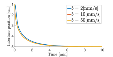
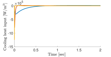
Figure 2: The closed-loop response of the interface position. For each operating speed, the interface position is stabilized after 6[min].

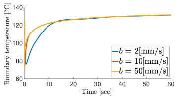
Figure 3: The closed-loop response of the output feedback control. The transient gets shorter as the operation gets faster.

Figure 4: The response of the boundary temperature, which maintains reasonable value for the material and safe operation.

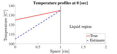
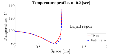
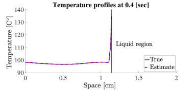
Figure 5: The comparison of the true and estimated temperature profiles.

For numerical study to investigate the controller’s performance in different operating conditions, we have employed the simulation of the original ”two-phase” model governed by (2)–(5) without assuming that the liquid phase is at stead-state, run the PDE observer given in (1)–(30), and implemented the associated output feedback controller (5.2). We used the boundary immobilization method to obtain a fixed boundary system and discretized the system with finite differnces to construct a finite dimensional representation of the model. Using Matlab’s ode23s solver, we simulated the setup with three different advection speeds ranging from 2 mm/s to 50 mm/s, to cover a wide spectrum of operating modes. The material parameters are chosen from [30], in which distinct values for high density polyethylene in solid and liquid state were experimentally derived (see Table 1). The extruder length is $L=10\,\mathrm{cm}$ and the constant barrel temperature is set to $T_{{\rm b}}=145\,\mathrm{{}^{\circ}C}$. Further, the auxiliary heat input was chosen $q_{\rm{m}}^{*}=100\,\nicefrac{\mathrm{W}}{\mathrm{m^{2}}}$. The initial temperature is set as a linear profile, which satisfies the boundary condition (4). For each advection speed, the control parameter $c$ is adjusted to generate a reasonable boundary temperature. While higher advection speeds enable shorter convergence times, it is only achieved when the control gain $c$ is also sufficiently large. However, larger values in the control gain will initially produce very low boundary temperature values. For each configuration, we adjusted the control gain as $c=$0.2 for $b=$2[mm/s], $c=$1.0 for $b=$10[mm/s], and $c=$5.0 for $b=$50[mm/s], to produce comparable temperature peaks at the inlet and prevent unrealistic values. The closed-loop responses of the interface position $s(t)$, the boundary control input $q_{{\rm f}}(t)$, and the boundary temperature $T_{{\rm s}}(0,t)$ are shown in Fig. 4, Fig. 4 and Fig. 4, respectively. The interface responses, depicted in Fig. 4, have quite similar behaviors in all three setups. However, the control input, shown in Fig. 4, appears to act faster for higher advection speeds but exhibits a similar qualitative behavior. Similar properties were observed in the boundary temperature response in Fig.4. Note that all the three figures have different time ranges.

Moreover, for the fast operating condition $b=$50[mm/s], the comparison of the estimated temperature profile and the true temperature profile at $t=$0[sec], 0.2[sec], 0.4[sec] are shown in Fig. 5. We can observe that the estimated temperature profile gets almost same as the true temperature profile at 0.4[sec], associated with the expansion of the solid granules’ region. Hence, the convergence of the designed observer to the true temperature profile is approximately 1000 times faster than the convergence of the interface position to the setpoint position, which is sufficiently quick performance of the temperature estimation.

For comparison, we also tested a closed loop setup with PI control given by

$$q_{\rm{f}}(t)=q_{\rm{f}}^{*}+K_{\rm{P}}(s(t)-s_{\rm{r}})+K_{\rm{I}}\int_{t_{0}}^{t}(s(\tau)-s_{\rm{r}})d\tau,$$ (133)

where $K_{\rm{P}}$ and $K_{\rm{I}}$ are gain parameters to be tuned in order to achieve the desired performance. However, for any choice of the parameters we have tried, the closed-loop response of the interface position does not stabilize at the sepoint $s_{{\rm r}}$. Fig. 6 depicts the responses under PI control with a relatively suitable choice of the gains. The lower plot in Fig. 6 shows that the temperature at the inlet of the extruder gets above the melting temperature at approximately 2.9 [min], which violates the validity condition (7) of the solid polymer temperature, while our proposed output feedback control guarantees to satisfy the condition under the closed-loop system. Such an overshoot behavior beyond the melting temperature might be reduced by PID control, however, the velocity of the interface position is nearly impossible to measure online and the differentiator generally causes high noise. Overall, the proposed output feedback control law illustrates superior performance to PI control in terms of both convergence to the setpoint and the validity condition.

From the simulations, we conclude that our control design achieves a stable interface position, even with very fast advection speeds 50 mm/s, with which a particle inserted in the inlet will travel in two seconds through the extruder, when assuming a 10 cm extruder.

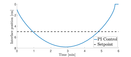
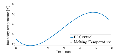
Figure 6: The response with PI control. The boundary temperature is heated up and gets above the melting temperature, which violates the condition for the solid phase temperature.

8 Conclusions

In this paper, we designed an observer and the associated output feedback control to stabilize an ink production process of the screw extrusion based 3D printing. The steady-state analysis is provided by setting the setpoint as a , and the control design to stabilize the interface position is derived. The simulation results prove the effectiveness of the boundary feedback control law for some given screw speeds.

References

- [1] S. Bukkapatnam and B. Clark, “Dynamic modeling and monitoring of contour crafting - An extrusion-based layered manufacturing process,” In Journal of manufacturing Science and Engineering, 129(1), pages 135-142. ASME 2007.
- [2] Riaz, M.N. “Extruders in Food Applications,” In Boca Raton: CRC Press, 240 pages, 2000.
- [3] Fang, Q., Hanna, M. and Lan, Y. “Extrusion system components,” In In: Heldman D. R. Ed., Encyclopedia of Agricultural, Food, and Biological Engineering, CRC Press, pages 301-305, 2003.
- [4] M. Diagne, N. Bekiaris-Liberis and M. Krstic, “Time- and State-Dependent Input Delay-Compensated Bang-Bang Control of a Screw Extruder for 3D Printing” In International Journal of Robust and Nonlinear Control, DOI: 10.1002/rnc.
- [5] M. Diagne, P. Shang and Z. Wang, “Feedback Stabilization of a Food Extrusion Process Described by 1D PDEs Defined on Coupled Time-Varying Spatial Domains” In Proceedings of the 13th IFAC Workshop on Time-Delay Systems, vol. 48, no. 12, 2015, pages 51-56, IFAC, 2015.
- [6] M. Diagne, P. Shang and Z. Wang, “Feedback Stabilization for the Mass Balance Equations of an Extrusion Process,” In IEEE Transactions on Automatic Control, vol. 61, no. 3, pp. 760-765, 2016.
- [7] D. Drotman, M. Diagne, R. Bitmead and M. Krstic, “Control-Oriented Energy-Based Modeling of a Screw Extruder Used for 3D Printing,” In 2016 Dynamic Systems and Control Conference, volume 1001, pages 48109. ASME, 2016.
- [8] R. Escobedo and L. Fernández, “Classical One-Phase Stefan Problems for Describing Polymer Crystallization Processes,” In SIAM Journal on Applied Mathematics, pages 254-280. SIAM, 2013.
- [9] S. Gupta, “The classical Stefan problem. Basic concepts, Modeling and Analysis,” In Applied Mathematics and Mechanics. North Holland, 2003
- [10] S. Koga, M. Diagne, S. Tang, and M. Krstic, “Backstepping control of the one-phase stefan problem,” In 2016 American Control Conference (ACC), pages 2548–2553. IEEE, 2016.
- [11] S. Koga, M. Diagne, and M. Krstic, “Output feedback control of the one-phase Stefan problem,” In 55th Conference on Decision and Control (CDC), pages 526–531. IEEE, 2016.
- [12] S. Koga, M. Diagne, and M. Krstic, “Control and state estimation of the one-phase Stefan problem via backstepping design,” IEEE Transactions on Automatic Control, vol. 64, no. 2, pp. 510–525, 2019.
- [13] S. Koga, R. Vazquez and M. Krstic, “Backstepping control of the Stefan problem with flowing liquid,” In 2017 American Control Conference (ACC), pages 1151-1156. IEEE 2017
- [14] S. Koga, L. Camacho-Solorio, and M. Krstic, “State Estimation for Lithium Ion Batteries With Phase Transition Materials,” —n ASME 2017 Dynamic Systems and Control Conference, American Society of Mechanical Engineers, 2017.
- [15] S. Koga and M. Krstic, “Delay compensated control of the Stefan problem,” In 56th Conference on Decision and Control (CDC), pp. 1242-1247, IEEE, 2017.
- [16] S. Koga, I. Karafyllis, and M. Krstic, “Input-to-State Stability for the Control of Stefan Problem with Respect to Heat Loss at the Interface,” In 2018 American Control Conference (ACC), pages 1740–1745. IEEE, 2018.
- [17] S. Koga, D. Straub, M. Diagne, and M. Krstic, “Thermodynamic Modeling and Control of Screw Extruder for 3D Printing,” In 2018 American Control Conference (ACC), pages 2551–2556. IEEE, 2018.
- [18] S. Koga and M. Krstic, “Control of Two-Phase Stefan Problem via Single Boundary Heat Input,” In 57th Conference on Decision and Control (CDC), pp. 2914-2919, IEEE, 2018.
-
[19]
S. Koga, D. Bresch-Pietri, and M. Krstic,
“Delay compensated control of the Stefan problem and robustness to delay mismatch,”
Preprint, available at
http://arxiv.org/abs/1901.09809, 2019. -
[20]
S. Koga, and M. Krstic,
“Arctic Sea Ice State Estimation From Thermodynamic PDE Model,”
Preprint, available at
https://arxiv.org/abs/1901.10678, 2019. - [21] M. Krstic and A. Smyshlyaev, Boundary Control of PDEs: A Course on Backstepping Designs. Singapore: SIAM, 2008.
- [22] M. Krstic, “Compensating actuator and sensor dynamics governed by diffusion PDEs,” Systems & Control Letters, vol. 58, pp. 372–377, 2009.
- [23] M. Kulshreshtha, C. Zaror and D. Jukes, “An unsteady state model for twin screw extruders,” In Tran IChemE, TartC, vol70, pages 21-28, 1995.
- [24] C. Ladd, J. H. So, J. Muth, and M.D. Dickey, “3D printing of free standing liquid metal microstructures,” In Advanced Materials, 25(36), pages 5081-5085, 2013.
- [25] C.-H. Li, “Modelling Extrusion Cooking” In Mathematical and Computer Modelling 33, pages 553-563. PERGAMON, 2001
- [26] V. Mironov, T. Boland, T. Trusk, G. Forgacs, and R.R. Markwald (2003). “Organ printing: computer-aided jet-based 3D tissue engineering” In TRENDS in Biotechnology, 21(4), pages 157-161. ELSEVIER 2003.
- [27] O. A. Mohamed, S. H. Masood, and J. L. Bhowmik, “Optimization of fused deposition modeling process parameters: a review of current research and future prospects,” In Advances in Manufacturing, 3(1), pages 42-53. Springer 2015.
- [28] D.H. Morton-Jones, “Polymer processing,” Chapman and Hall London, 1989
- [29] H. Seitz, W. Rieder, S. Irsen, B. Leukers, and C. Tille, “Three‐dimensional printing of porous ceramic scaffolds for bone tissue engineering,” In Journal of Biomedical Materials Research Part B: Applied Biomaterials, 74(2), pages 782-788, 2005
- [30] Z. Tadmor and C. Gogos “Principles of polymer processing,” John Wiley & Sons, 2006.
- [31] H. Valkenaers, F. Vogeler, E. Ferraris, A. Voet and J. Kruth “A novel approach to additive manufacturing: Screw extrusion 3D-printing,” In Proceedings of the 10th International Conference on Multi-Material Micro Manufacture, pages 235-238. Research Publishing, 2013.
- [32] B. Vergnes, G.D. Valle, and L. Delamare, “A global computer software for polymer flows in corotating twin screw extruders,” Polymer Engineering & Science, 38(11), pp.1781-1792, 1998.
- [33] J. L. White, E. K. Kim, J. M. Keum, H. C. Jung and D. S. Bang, “Modeling heat transfer in screw extrusion with special application to modular self‐wiping co‐rotating twin‐screw extrusion,” In Polymer Engineering & Science, 41(8), pages 1448-1455, 2001.