Noncommutative phase-space effects in thermal diffusion of Gaussian states

Abstract

Noncommutative phase-space and its effects have been studied in different settings in physics, in order to unveil a better understanding of phase-space structures. Here, we use the thermal diffusion approach to study how noncommutative effects can influence the time evolution of a one-mode Gaussian state when in contact with a thermal environment obeying the Markov approximation. Employing the cooling process and considering the system of interest as a one-mode Gaussian state, we show that the fidelity comparing the Gaussian state of the system in different times and the asymptotic thermal state is useful to sign noncommuative effects. Besides, by using the monotonicity behavior of the fidelity, we discuss some aspects of non-Markovianity during the dynamics.

1 Introduction

Quantum dissipative systems is a research field broadly investigated in theoretical and experimental physics because they are one of the best examples of open quantum system applications Petruccione01 ; Rivas01 . There is a fairly deep interest in dissipative acting on quantum systems, ranging from quantum optics to condensed matter physics as, for instance, entangled states in optical cavities Reiter , dissipative optomechanical systems Liew , in the Rabi model Plenio01 , and in systems interacting with Gaussian dissipative reservoir Marcin . Besides, there exist a practical appeal to control dissipation in quantum technologies, such as quantum information processing Pleni02 and quantum computation Zureck01 . Then, in general, one can think that dissipation comes from the interaction of quantum systems to some external agent, such as a thermal environment.

On the other hand, from a theoretical point of view, exciting questions arise when new quantum features can affect quantum thermodynamic processes, in particular, that features underlying the context of phase-space noncommutativity (NC) extension of quantum mechanics. The noncommutativity in the configuration space has been firstly suggested by Snyder Snyder as a propose to avoid divergences in the quantum field theory. Additionally, there is a fairly deep consensus that in the Planck scale $(\sim 10^{-32}cm)$, the notion of space-time has to be drastically rectified in a consistent formulation of quantum mechanics and gravity ref01 ; ref02 , such that noncommutativity must be assumed at high energy scales. There is a large number of studies concerning the implications of what has been conventionally called by noncommutative quantum mechanics (NCQM), for instance, in the context of $2D$-harmonic oscillator Vergara ; Bernardini01 , the gravitational quantum well Orfeu01 ; Banerjee ; extra01 , and in relativist dispersion relations Leal01 .

In the context of experimental verification of signatures of noncommutative effects, it is worth to mention that current experimental range is far away from the Planck scale and, at this moment is not clear how to reach this experimental ability. However, some recent theoretical developments in this direction have arisen, for instance, using quantum optics extra02 and opto-mechanical extra03 setups. In particular, Ref. extra02 employs a quantum mechanical ancillary system that can work in order to measure any deformation of the canonical commutator directly, by means of an additional optical phase that is absent in the standard quantum mechanics. Moreover, some theoretical studies have been done exploring noncommutative effects in master equation, in particular for the Brownian particle extra06 . In the direction of these recent developments, we could argue that some tools from information theory would be suitable to sign noncommutative effects in open quantum systems. For instance, the quantum fidelity is a good measure to indicate any non-trivial signature in the dynamics of a system evolving in thermal contact with an environment.

It can be observed that for systems described by Hamiltonians at most quadratic in their coordinates, the noncommutative effects can be effectively mapped to the standard quantum mechanics as an external magnetic field acting on the system Bernardini01 ; Jonas00 ; Jonas01 ; Jonas02 . This fact allows to obtain a convenient correspondence between the NCQM and the standard quantum mechanics (SQM) which is suitable to investigate how NC effects could impact some particular dynamics. The aim of this work is to use this property to study how NC effects can influence a thermalization process. We considered the so called Gaussian states as our system evolving under the dynamics of the NC harmonic oscillator. Then, we put the system in a contact with a thermal environment in order to probe how the time evolution of the system state is influenced by NC effects. We assume the cooling process, i. e., the system and the thermal environment are associated to the mean numbers of photons $\bar{n}$ and $\bar{m}$, respectively, such that $\bar{n}>\bar{m}$. To quantify our study we use the quantum fidelity which has a well known form when both states are Gaussian.

This work is organized as follows. In section 2 we introduce the necessary information on noncommutative quantum mechanics and the Seiberg-Witten map. Besides, we provide the theoretical framework to treat thermal diffusion of Gaussian states. In particular, the section 3 is devoted to show how to map NC effects as effective external fields acting on the harmonic oscillator Hamiltonian and its equations of motion. Section 4 is dedicated to show how NC effects can affect the cooling dynamics of a Gaussian state when in contact with a thermal environment. Finally, in section 5 we draw our conclusions and final remarks.

2 Theoretical Framework

In this section we provide the theoretical framework to treat noncommutativity in phase-space and the thermal diffusion equation for Gaussian states.

2.1 Noncommutative quantum mechanics in phase-space

Noncommutative quantum mechanics is based on the deformed Heisenberg-Weyl algebra Bernardini01 ; Orfeu01 ; Orfeu02 ; Gamboa and it is represented by the commutation relations given by,

$$\small\left[\hat{q}_{i},\hat{q}_{j}\right]=i\theta_{ij},\,\left[\hat{q}_{i},\hat{p}_{j}\right]=i\hbar\delta_{ij},\,\left[\hat{p}_{i},\hat{p}_{j}\right]=i\zeta_{ij},\quad i,j=1,...,d,$$ (1)

where $\theta_{ij}$ and $\zeta_{ij}$ are invertible antisymmetric real constant $(d\times d)$ matrices, and one can define the matrix $\Sigma_{ij}=\delta_{ij}+\theta_{ik}\zeta_{kj}/\hbar^{2}$, which is also invertible if $\theta_{ik}\xi_{kj}\neq-\hbar^{2}\delta_{ij}$. Writing $\theta_{ij}=\theta\epsilon_{ij}$ and $\zeta_{ij}=\zeta\epsilon_{ij}$, with $\epsilon_{ii}=0$, $\epsilon_{ij}=-\epsilon_{ji}$, one can interpret $\eta$ and $\zeta$ as being new constants in the quantum theory, which have been extensively studied recently Bernardini01 ; Jonas02 ; Saha ; Bastos ; Bastos02 ; Andreas . Furthermore, there is a way of connecting the Hilbert space of the NCQM to that of the SQM, which is represented by the following relations,

$$\small\left[\hat{Q}_{i},\hat{P}_{j}\right]=0,\,\left[\hat{Q}_{i},\hat{P}_{j}\right]=i\hbar\delta_{ij},\,\left[\hat{P}_{i},\hat{P}_{j}\right]=0,\quad i,j=1,...,d.$$ (2)

This is implemented through the Seiberg-Witten (SW) map, given by $\hat{q}_{i}=\nu\hat{Q}_{i}-(\theta/2\nu\hbar)\epsilon_{ij}\hat{P}_{j}$ and $\hat{p}_{i}=\mu\hat{P}_{i}+(\zeta/2\mu\hbar)\epsilon_{ij}\hat{Q}_{j}$, where $\nu$ and $\mu$ are arbitrary parameters fulfilling the condition $\theta\zeta=4\hbar^{2}\mu\nu(1-\mu\nu)$.

Once the SW map is applied to the Hamiltonian of a system, to describe the state of such a system, one can use the density matrix $\hat{\rho}=|\Psi\rangle\langle\Psi|$ , which can be used to define the associated Wigner function through the Weyl transform Case ; Zachos ,

$$W(Q_{i},P_{i}) = h^{-1}\rho^{W}$$

$$= h^{-1}\int dy\,exp[iPy/\hbar]\Psi(Q_{i}-y/2)\Psi(Q_{i}+y/2),$$

which can be naturally generalized to a statistical mixture, with “W” standing for the Weyl transform. The marginal integration of the Wigner function results in,

$$\psi^{\star}(Q_{i})\psi(Q_{i}) =\int dP_{i}\,W(Q_{i},P_{i})$$ (3)

$$\psi^{\star}(P_{i})\psi(P_{i}) =\int dQ_{i}\,W(Q_{i},P_{i}),$$ (4)

i. e., the probability distribution for position and momentum, respectively. The Wigner function can be used to obtain the expectation value of an observable $\mathcal{\hat{\mathcal{O}}}$ as,

$$\langle\mathcal{O}\rangle=\int\int dQ_{i}dP_{i}\,W(Q_{i},P_{i})\mathcal{O}^{W}(Q_{i},P_{i}).$$ (5)

where $\mathcal{O}^{W}(Q_{i},P_{i})$ is the Weyl transform of the operator $\hat{\mathcal{O}}$.

2.2 Gaussian States and Thermal Diffusion

One important class of states with extensive theoretical and experimental applications are the so called Gaussian states (GS) which has been largely used in quantum information and quantum communication Adesso ; Wang , quantum metrology Adesso02 , quantum optics Walls etc. Gaussian states are a subset of the more general class used to treat continuous variables (CV) systems Wang ; extra05 ; Adesso . An important aspect of the GS is that they are completely characterized by their first and second moments. Introducing a vector $\vec{R}(Q_{1},P_{1},Q_{2},P_{2})$ to collect the coordinates of a two-dimensional system, the first moments can be rearranged in the vector $\vec{d}=(\langle Q_{1}\rangle,\langle P_{1}\rangle,\langle Q_{2}\rangle,\langle P_{2}\rangle)$. The set of all second moments are collected in the so called covariance matrix (CM), given by $\sigma=\sigma_{11}\oplus\sigma_{22}$ for a two-mode Gaussian state, where,

$$\sigma_{ii}=\left(\begin{array}[]{cc}\sigma_{Q_{i}Q_{i}}&\sigma_{P_{i}Q_{i}}\\ \sigma_{Q_{i}P_{i}}&\sigma_{P_{i}P_{i}}\end{array}\right),$$ (6)

with $\sigma_{AB}=\langle AB+BA\rangle-2\langle A\rangle\langle B\rangle$. It can be shown that for a bona-fide two-mode Gaussian state the CM satisfies the relation $\sigma+i\Omega\geq 0$, where,

$$\Omega=\left(\begin{array}[]{cc}0&1\\ -1&0\end{array}\right)^{\oplus 2},$$ (7)

such that $\left[\vec{R}_{i},\vec{R}_{j}\right]=i\Omega_{ij}$ Simon . In particular, for GS the Wigner function assumes a gently form given by Adesso ,

$$W_{G}(\vec{R})=\frac{\text{exp}\left[-(1/2)(\vec{R}-\vec{d})\sigma^{-1}(\vec{R}-\vec{d})\right]}{(2\pi)^{2n}\sqrt{Det[\sigma]}},$$ (8)

where $n$ is the number of modes of the system. A special type of GS is the thermal state. A one-mode thermal state is represented by Adesso ,

$$\rho^{th}(\bar{m})=\sum_{m=0}^{\infty}\frac{\bar{m}^{m}}{(\bar{m}+1)^{m+1}}|m\rangle\langle m|,$$ (9)

where $\bar{m}=\left\{exp\left[\hbar\omega/k_{B}T\right]-1\right\}^{-1}$ is the mean number of photons in the bosonic mode, $k_{B}$ is the Boltzmann constant, $T$ is the associated temperature, and $\{|m\rangle\}$ is the Fock basis, with first moments and CM given by $\vec{R}=(0,0)$ and $\sigma^{th}=(2\bar{m}+1)\mathbb{I}_{2\times 2}$, respectively, where $\mathbb{I}_{2\times 2}$ represents a two-by-two identity matrix.

The propagation of a general Gaussian state in a noisy and dissipative channel where each mode is coupled with a different and uncorrelated Markovian environment modeled by a stationary continuum of oscillators can be described, in the interaction picture, by the following master equation,

$$\frac{d}{dt}\rho=-i\left[\hat{H},\hat{\rho}\right]+\mathcal{L}(\hat{\rho}),$$ (10)

where the first and second term on the right-hand side represent the unitary and dissipative part of the dynamics. It can be shown that when the system of interest is a Gaussian state the dynamics is easily evolved in terms of the first moments and covariance matrix Serafini ; Giovanneti01 ,

$$\dot{\sigma} = \Gamma\sigma+\Gamma(2\bar{m}+1)\mathbb{I}_{2\times 2},$$

$$\dot{\vec{d}} = -(\Gamma/2)\vec{d},$$

with solutions,

$$\sigma(t) =e^{-\Gamma t}\sigma(0)+(1-e^{-\Gamma t})(2\bar{m}+1)\mathbb{I}_{2\times 2},$$ (11)

$$\vec{d}(t) =e^{-\Gamma t/2}\vec{d}(0),$$ (12)

where $\Gamma$ is the decay rate and $\bar{m}$ is the mean number of photons of the thermal environment, and $\sigma(0)$ and $\vec{d}(0)$ are the initial covariance matrix and first moments of the system. Assuming a mean number of photons to the system as being $\bar{n}$, we remark that for the cooling process, $\bar{n}>\bar{m}$, whereas for the heating process, $\bar{n}<\bar{m}$. Here, we adopt the cooling process to investigate the NC effects. To conclude this section, we are interested in the time evolution of the following two-dimensional Gaussian Wigner function,

$$\small W_{G}(\vec{R}) = \frac{1}{\pi^{2}}\text{exp}\left[-\left((Q_{1}(t)-x_{0})^{2}-(Q_{2}(t)-y_{0})^{2}\right)\right]$$ (13)

$$\times \text{exp}\left[-\left((P_{1}(t)-p_{y_{0}})^{2}-(P_{2}(t)-p_{y_{0}})^{2}\right)\right],$$

where $x_{0}$,$y_{0}$, $p_{x_{0}}$ and $p_{y_{0}}$ are arbitrary initial parameters.

3 Mapping Noncommutative Effects as External Fields

Let us consider the Hamiltonian of a noncommutative harmonic oscillator,

$$\hat{H}^{NC}(\hat{q}_{i},\hat{p}_{i})=\frac{\hat{p}_{i}^{2}}{2m}+\frac{m\omega^{2}}{2}\hat{q}_{i}^{2},$$ (14)

where $m$ and $\omega$ are the mass and frequency of the system, respectively. Applying the SW map to obtain the standard version of the eq.(14) and then performing the Weyl transform, one gets Vergara ; Bernardini01 ,

$$H(Q_{i},P_{i})=\alpha^{2}Q_{i}^{2}+\beta^{2}P_{i}^{2}+\gamma\sum_{i,j=1}^{2}\epsilon_{ij}P_{i}Q_{j},$$ (15)

where we defined,

$$\small\alpha^{2}=\frac{\nu^{2}m\omega^{2}}{2}+\frac{\zeta^{2}}{8m\mu^{2}\hbar^{2}},\,\beta^{2}=\frac{\mu^{2}}{2m}+\frac{m\omega^{2}\theta^{2}}{8\nu^{2}\hbar^{2}},\,\gamma=\frac{\theta}{2\hbar}m\omega^{2}+\frac{\zeta}{2m\hbar}.$$ (16)

Following ref. Bernardini01 , we use the Heisenberg equation to obtain a set of uncoupled four equations of motions,

$$Q_{1}(t) = x_{0}\cos(\Omega t)\cos(\gamma t)+y_{0}\cos(\Omega t)\sin(\gamma t)$$ (17)

$$+ \frac{\beta}{\alpha}[p_{y_{0}}\sin(\Omega t)\sin(\gamma t)+p_{x_{0}}\sin(\Omega t)\cos(\gamma t)]$$

$$Q_{2}(t) = y_{0}\cos(\Omega t)\cos(\gamma t)-x_{0}\cos(\Omega t)\sin(\gamma t)$$ (18)

$$- \frac{\beta}{\alpha}[p_{x_{0}}\sin(\Omega t)\sin(\gamma t)-p_{y_{0}}\sin(\Omega t)\cos(\gamma t)]$$

$$P_{1}(t) = p_{x_{0}}\cos(\Omega t)\cos(\gamma t)+p_{y_{0}}\cos(\Omega t)\sin(\gamma t)$$ (19)

$$- \frac{\alpha}{\beta}[y\sin(\Omega t)\sin(\gamma t)+x\sin(\Omega t)\cos(\gamma t)]$$

$$P_{2}(t) = p_{y_{0}}\cos(\Omega t)\cos(\gamma t)-p_{x_{0}}\cos(\Omega t)\sin(\gamma t)$$ (20)

$$+ \frac{\alpha}{\beta}[x_{0}\sin(\Omega t)\sin(\gamma t)-y_{0}\sin(\Omega t)\cos(\gamma t)],$$

where $\Omega=2\alpha\beta=\omega\sqrt{(2\mu\nu-1)^{2}+\xi^{2}}$ and $\xi=(1/2\hbar)\left[m\omega\theta+\zeta/(m\omega)\right]$.

From eq.(15) we can note that the influence of the noncommutative parameters $\theta$ and $\zeta$ on the dynamics of the system is effectively a magnetic field-like term in the orthogonal direction to the plane of the oscillator. More explicitly, from the Hamiltonian of a harmonic oscillator in an external magnetic field Rob , one has,

$$B_{0}\sim\frac{m^{2}\omega^{2}\theta}{q\hbar}+\frac{\zeta}{q\hbar},$$ (21)

where $q$ is the effective charge associated to the harmonic oscillator.

4 Thermal Diffusion with NC Effects

In order to see how NC effects can influence the thermal diffusion process, we consider a Gaussian Wigner function as in eq.(13) evolving onto the dynamics dictated by eqs.(17-20). Assuming we are interested in the phase-space $\left(Q_{1},P_{1}\right)$ as our system, the respective Wigner function is obtained tracing out the coordinates $\left(Q_{2},P_{2}\right)$, i. e.,

$$W_{sys}(Q_{1},P_{1})=\int_{-\infty}^{\infty}\int_{-\infty}^{\infty}dQ_{2}dP_{2\,}W_{G}(\vec{R})=W_{1}$$ (22)

It is important to stress that $W_{sys}(Q_{1},P_{1})$ will be Gaussian during all the time evolution, such that we can assume that the first moments and the covariance matrix are sufficient to characterize the state of the system and they are given by $\langle\vec{d}_{sys}\rangle$ and $\sigma_{sys}$, i. e.,

$$\small\langle\vec{d}_{sys}\rangle=(\langle Q_{1}\rangle_{W_{1}},\langle P_{1}\rangle_{W_{1}}),\,\sigma_{sys}=\left(\begin{array}[]{cc}\langle\sigma_{Q_{1}Q_{1}}\rangle_{W_{1}}&\langle\sigma_{P_{1}Q_{1}}\rangle_{W_{1}}\\ \langle\sigma_{Q_{1}P_{1}}\rangle_{W_{1}}&\langle\sigma_{P_{1}P_{1}}\rangle_{W_{1}}\end{array}\right),$$ (23)

where $\langle\sigma_{AB}\rangle_{W_{1}}=\langle AB+BA\rangle_{W_{1}}-2\langle A\rangle_{W_{1}}\langle B\rangle_{W_{1}}$ and the mean values are obtained over the Wigner function $W_{1}$.

After that, the system is placed in thermal contact with an environment represented by a mean number of photons $\bar{m}$, such that the first moments are null and $\sigma^{th}(\bar{m})=(2\bar{m}+1)\mathbb{I}_{2\times 2}$. For an environment fulfilling the Born-Markovian approximation, we assume a decay rate $\Gamma$. Besides, we consider $\langle\hat{B}_{i}^{\dagger}(0)\hat{B}_{i}(\nu)\rangle=\bar{m}\delta(\nu)$ and $\langle\hat{B}_{i}(0)\hat{B}_{i}(\nu)\rangle=M\delta(\nu)$, where $\hat{B}$ is the bosonic operator associated to the environment and the second expression relates the squeezing feature of the environment. Here, we assume that $M=0$, i. e., the environment is just a thermal one. Furthermore, we consider that the thermal environment interacts only with the sub-space $(Q_{1},P_{1})$ or, in other words, the interaction between the sub-space $(Q_{2},P_{2})$ and the thermal environment is sufficiently week such that it does not cause any effects on the evolution of the state $W_{sys}(Q_{1},P_{1}).$ During the time evolution of the system in contact with the thermal environment, we assume the cooling process, i. e., we indexed to the system a mean number of photons $\bar{n}$, with $\bar{n}>\bar{m}$ and, for a Markovian evolution, $\bar{n}\rightarrow\bar{m}$ for a time sufficiently large. The time evolution of the first moments and CM during the thermal diffusion reads,

$$\sigma_{sys}(t) =\bar{n}e^{-\Gamma t}\sigma_{sys}(0)+(1-e^{-\Gamma t})(2\bar{m}+1)\mathbb{I}_{2\times 2},$$ (24)

$$\vec{d}_{sys}(t) =e^{-\Gamma t/2}\vec{d}_{sys}(0).$$ (25)

In order to quantify how NC effects mapped effectively as external fields influence the cooling process, we use the quantum fidelity which, for two Gaussian states, has the well known expression Holevo ; Scutaru ; extra04 ,

$$F(\sigma_{1},\vec{d}_{1};\sigma_{2},\vec{d}_{2})=\frac{2}{\sqrt{\Delta+\delta}-\sqrt{\delta}}e^{-\frac{1}{2}\vec{d}^{T}\sigma_{+}^{-1}\vec{d}},$$ (26)

where $\Delta\equiv Det[\sigma_{1}+\sigma_{2}]$, $\delta=(Det[\sigma_{1}]-1)(Det[\sigma_{2}]-1)$, $\vec{d}\equiv\vec{d}_{1}-\vec{d}_{2}$, and $\sigma_{+}=\sigma_{1}+\sigma_{2}$. The fidelity is bounded by $0\leq F\leq 1$, with $F=0$ for two completely different states and $F=1$ for two identical states. Here we consider $(\sigma_{1},\vec{d}_{1})$ and $(\sigma_{2},\vec{d}_{2})$ as being our system of interest during the time evolution and the asymptotic thermal state for complete cooling, respectively.

Figure 1: (Color online) Quantum fidelity as a function of time for the Gaussian state of the system $(Q_{1}P_{1})$ and the asymptotic thermal state for complete cooling, for a initial state of the system displaced from the origin, $(x_{0},p_{x_{0}})=(1,1)$ ( figure (a)), and for a initial state of the system initially in the origin, $(x_{0},p_{x_{0}})=(0,0)$ (figure (b)). The parameter $\tau$ is inserted just to have a dimensionless variable; we choose a decay rate $\Gamma=0.1\tau$ and $\bar{n}=4$ and $\bar{m}=2$, such that we have the cooling process.

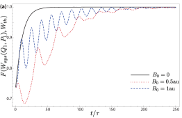
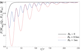
In Fig. 1 we have plotted the quantum fidelity as a function of time for the Gaussian state of the system $(Q_{1},P_{1})$ and the asymptotic thermal state for complete cooling, assuming $(\bar{n},\bar{m})=(4,2)$ in order to have the cooling process of the system. We consider three different cases, i. e., the absence of NC effects, $B_{0}=0$ (black, solid line) and two cases with NC effects represented by $B_{0}=0.5$au (red, dotted line) and $B_{0}=1$au (blue, dashed line) where au means arbitrary unity. Moreover, two initially located system states were assumed: $(x_{0},p_{x_{0}})=(1,1)$ (figure (a)) and $(x_{0},p_{x_{0}})=(0,0)$ (figure (b)). The black curves corresponds exactly to the process of cooling of a Gaussian state when in contact with a thermal environment, i. e., the fidelity increases monotonically up to unity. The only difference is the initial value of the fidelity, which is easily explained by noting that in the second case the system starts the dynamics with $(\vec{d}_{sys})=(0,0)$, i. e., it is more closely to the asymptotic state for complete cooling process. For $B_{0}\neq 0$, we observe that the monotonicity of the fidelity is not fulfilled, though as the time increases the state of the system goes to the asymptotic state. It can be also noted a difference of phase relative to the two values of $B_{0}$ when we change the initial position of the system in the phase-space.

Non-Markovian-like Effect

As we can note from the time evolution of the quantum fidelity in Fig. 1, for $B_{0}\neq 0$ the fidelity does not increase monotonically up to unity. The presence of oscillations in the fidelity during a thermalization process has been largely studied in the literature as been associated to an information backflow from the thermal environment to the system Rivas02 ; Breuer . Non-Markovian effects is a current field of research with several applications in quantum information Latune ; Luoma and quantum thermodynamics Marcantoni ; Maniscalco02 , both in theoretical and experimental areas Breuer03 . As we have mentioned above, quantum fidelity obeys a significant property, i. e., monotonicity Nielsen ,

$$F(\Lambda\rho_{1},\Lambda\rho_{2})\geq F(\rho_{1},\rho_{2}),$$ (27)

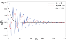
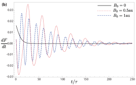
where $\Lambda$ denotes a completely positive map, which serves as a characteristic feature of Markovian dynamics (see Fig. 1). Noticing that Markovian evolution guarantees a completely positive trace preserving dynamical map $\Lambda(t)$, i. e., $\rho(0)\rightarrow\rho(t)=\Lambda(t)\rho(0)$, which also forms a one-parameter semigroup obeying the composition law kraus : $\Lambda(t_{1})\Lambda(t_{2})=\Lambda(t_{1}+t_{2})$, with $t_{1},t_{2}\geq 0$. Therefore, any violation of the inequality in Eq. (27) is a clear signature of non-Markovian dynamics, indicating that the associated dynamical map does not obey the composition law. It is worth to mention that deviation from (27) is sufficient, though not necessary, reflection of non-Markovianity. Following the standard procedure, we used the time derivative of the quantum fidelity to indicate what we call non-Markovian-like effect, i.e., an effective non-Markovian behavior due exclusively to $B_{0}\neq 0$. Therefore, for non-Markovian-like effect we have

$$\frac{d}{dt}F(\sigma_{1},\vec{d}_{1};\sigma_{2},\vec{d}_{2})<0.$$ (28)

In order to visualize this type of effect in our system, we depicted in Fig. 2 the time evolution of the time derivative presented in Fig. 1, using the same parameters. We note clearly the existence of non-Markovian-like effects during the cooling process. Obviously, the same effect would be present if the heating process was considered, i. e., $\bar{n}<\bar{m}$. From the Fig. 2 one can note that the intensity of the effect is greater as the intensity of the field increases when the system starts out of the origin, and the intensity of the effect is lower as the intensity of the field decreases when the system starts at the origin.

Figure 2: (Color online) Time derivative of the quantum fidelity for the same cases represented in Fig. (1). We considered three cases: $B_{0}=0$ (black, solid line), $B_{0}=0.5$au (red, dotted line), and $B_{0}=1$au (blue, dashed line). The same parameters of the Fig. (1) were used here.

It is important to worth that the thermal environment generates a Markovian dynamics on the system of interest. Then, any deviation from the Markovian profile described by the quantum fidelity must to have another source. Here, the only responsible source is the noncommutative effects mapped as effective external magnetic field.

5 Conclusions

In this work we used the possibility of mapping noncommutative effects as external fields to study how these effects can influence a cooling process of a system described by a Gaussian state. Using the well known thermal diffusion approach, we investigated the time evolution of the state of the system in two situations, first out of the origin and second at the origin of the phase-space, remembering that the asymptotic thermal state for complete cooling remains at the origin during the process. It can be observed that the evolution to the asymptotic state depends on the the value of $B_{0}$ and on the initial localization of the system in the phase-space. Besides, for $B_{0}\neq 0$ the system takes a longer time to reach the asymptotic state.

We also discuss the conceptual meaning of a non-Markovian-like effect during the time evolution of the system from an initial state to the asymptotic thermal state. It must be stressed that the thermal environment introduces a Markovian dynamics and that the decay rate $\Gamma$ does not depend on time. Therefore, the negativity of the time derivative of the quantum fidelity is exclusively due to $B_{0}\neq 0$. We believe that this work can contribute to unveil important features of noncommutative effects mapped as external fields on the dynamics of Gaussian states. Finally, in describing these effects through Gaussian states and thermal diffusion, studies concerning the experimental simulation of NC effects can emerge in the future.

References

- (1) H. P. Breuer and F. Petruccione, The Theory of Open Quantum Systems (Oxdord University Press, Oxford, 2002).
- (2) . Rivas and S. F. Huega, Open Quantum Systems. An Introduction (Springer, New York, 2012).
- (3) M. J. Kastoryano, F. Reiter, and A. S. S rensen, Dissipative Preparation of Entanglement in Optical Cavities, Phys. Rev. Lett. , 090502 (2011).
- (4) O. Kyriienko, T. C. H. Liew, and I. A. Shelykh, Optomechanics with Cavity Polaritons: Dissipative Coupling and Unconventional Bistability, Phys. Rev. Lett. , 076402 (2014).
- (5) A. Le Boite, M.-J. Hwang, and M. B. Plenio, Metastability in the driven-dissipative Rabi model, Phys. Rev. A , 023829 (2017).
- (6) M. Jarzyna and M. Zwierz, Parameter estimation in the presence of the most general Gaussian dissipative reservoir, Phys. Rev. A , 012109 (2017).
- (7) A. Bermudez, T. Schaetz, and M. B. Plenio, Dissipation-Assisted Quantum Information Processing with Trapped Ions, Phys. Rev. Lett. , 110502 (2013).
- (8) W. H. Zurek, Reversibility and Stability of Information Processing Systems, Phys. Rev. Lett. , 391 (1984).
- (9) H. S. Snyder, Phys. Rev. 71, 38 (1946).
- (10) S. Doplicher, K. Fredenhagen and J. E. Roberts, Commun. Math. Phys., 187 (1995).
- (11) N. Seiberg, “Emergent Spacetime”, arXiv:hep-th/0601234.
- (12) M. Rosenbaum and J. David Vergara, The star-value Equation and Wigner Distributions in Noncommutative Heisenberg algebras, Gen. Rel. Grav. 38, 607 (2006)
- (13) A. E. Bernardini and O. Bertolami, Probing phase-space noncommutativity through quantum beating, missing information and the thermodynamic limit, Phys. Rev. A , 012101 (2013).
- (14) O. Bertolami, J. G. Rosa, C. M. L. de Arag o, P. Castorina, and D. Zappal , Noncommutative Gravitational Quantum Well, Phys. Rev. D , 025010 (2005).
- (15) R. Banerjee, B. D. Roy, and S. Samanta, Remarks on the Noncommutative Gravitational Quantum Well, Phys. Rev. D74, 045015 (2006).
- (16) Kh. P. Gnatenko and V. M. Tkachuk, Upper bound on the momentum scale in noncommutative phase space of canonical type, ArXiv:1905.03245 (2019).
- (17) P. Leal and O. Bertolami, Relativistic dispersion relation and putative metric structure in noncommutative phase-space, Phys. Lett. B 793, 240 (2019).
- (18) S. Dey, A. Bhat, D. Momeni, M. Faizal, A. F. Ali, T.K. Dey and A. Rehman, Probing noncommutative theories with quantum optical experiments, Nucl. Phys. B 924, 578-587 (2017).
- (19) M. Khodadi, K. Nozari, S. Dey, A. Bhat and M. Faizal, A new bound on polymer quantization via an opto-mechancial setup, Nature Scientific Reports 8, 1659 (2018).
- (20) N. C. Dias and J. N. Prata, Exact master equation for a noncommutativeBrownian particle, Ann. Phys. 324 73 (2009).
- (21) J. F. G. Santos, A. E. Bernardini, and C. Bastos, Probing phase-space noncommutativity through quantum mechanics and thermodynamics of free particles and quantum rotors, Physica A , 340 (2015)
- (22) J. F. G. Santos and A. E. Bernardini, Gaussian fidelity distorted by external fields, Physica A , 75 (2016).
- (23) J. F. G. Santos and A. E. Bernardini, Quantum engines and the range of the second law of thermodynamics in the noncommutative phase-space, Eur. Phys. J. Plus , 260 (2017).
- (24) C.Bastos and O.Bertolami, Berry phase in the gravitational quantum well and the Seiberg–Witten map, Phys. Lett. A , 34 (2008).
- (25) J. Gamboa, M. Loewe, and J. C. Rojas, Phys. Rev. D , 067901 (2001).
- (26) A. Saha, S. Gangopadhyay, and S. Saha, Noncommutative quantum mechanics of a harmonic oscillator under linearized gravitational waves, Phys. Rev. D , 025004 (2011).
- (27) C. Bastos, N.C. Dias, and J.N. Prata, Wigner Measures in Noncommutative Quantum Mechanics, Commun. Math. Phys. , 3 (2010).
- (28) C. Bastos, O. Bertolami, and N. Dias, J. Prata, Noncommutative Graphene, Int. J. Mod. Phys. A , 16 (2013).
- (29) J. B. Geloun, F. G. Scholtz, Coherent states in noncommutative quantum mechanics, J. Math. Phys. , 043505 (2009).
- (30) W. B. Case, Wigner functions and Weyl transforms for pedestrians, Am. J. Phys. 76, 937 (2008).
- (31) C. K. Zachos, D. B. Fairlie e T. L. Curtright, Quantum Mechanics in PhaseSpace: An Overview with Selected Papers, (World Scientific, (World Scientific, Singapore, 2005).
- (32) X.-B. Wang, T. Hiroshima, A. Tomita, and M. Hayashi, Quantum information with Gaussian states, Phys. Rep. , 1 (2007).
- (33) C. Weedbrook, S. Pirandola, R. Garc a-Patr n, N. J. Cerf, T. C. Ralph, J. H. Shapiro, and Seth Lloyd, Gaussian quantum information, Rev. Mod. Phys. 84, 621 (2012).
- (34) G. Adesso, S. Ragy, and A. R. Lee, Continuous variable quantum information: Gaussian states and beyond, Open Syst. Inf. Dyn., 1440001 (2014).
- (35) R. Nichols, P. Liuzzo-Scorpo, P. A. Knott, and G. Adesso, Multiparameter Gaussian quantum metrology, Phys. Rev. A , 012114 (2018).
- (36) D. F. Walls and G. J. Milburn, Quantum Optics (Springer, Berlin, 2008).
- (37) R. Simon, E. E. G. Sudarsan, and N. Makunda, Gaussian-Wigner distributions in quantum mechanics and optics, Phys. Rev. A , 3868 (1987).
- (38) A. S. Holevo, Some statistical problems for quantum Gaussian states, IEEE Trans. Inf. Theory , 533 (1975).
- (39) H. Scutaru, Fidelity for displaced squeezed states and the oscillator semigroup, J. Phys. A , 3659 (1998).
- (40) L. Banchi, S. L. Braunstein, and S. Pirandola, Quantum Fidelity for Arbitrary Gaussian States, Phys. Rev. Lett. 115, 260501 (2015)
- (41) A. Serafini, Quantum Continuous Variables. A primer of Theoretical Methods, (CRC Press, Boca Raton, 2017).
- (42) A. Carlini, A. Mari, and V. Giovanneti, Time-Optimal Thermalization of Single-Mode Gaussian States, Phys. Rev. A , 052324 (2014).
- (43) R. Robinett, Quantum Mechanics: Classical Results, Modern Systems, and Visualized Examples, (Oxford University Press, Oxford, 2006).
- (44) . Rivas, S. F. Huelga, and M. B. Plenio, Entanglement and Non-Markovianity of Quantum Evolutions, Phys. Rev. Lett. , 050403 (2010).
- (45) H.-P. Breuer, E.-M. Laine, and J. Piilo, Measure for the Degree of Non-Markovian Behavior of Quantum Processes in Open Systems, Phys. Rev. Lett. , 210401 (2009).
- (46) C. L. Latune, I. Sinayskiy, and F. Petruccione, Quantum force estimation in arbitrary non-Markovian Gaussian baths, Phys. Rev. A , 052115 (2016).
- (47) N. Megier, W. T. Strunz, C. Viviescas, and K. Luoma, Parametrization and Optimization of Gaussian Non-Markovian Unravelings for Open Quantum Dynamics, Phys. Rev. Lett , 150402 (2018).
- (48) S. Marcantoni, S. Alipour, F. Benatti, R. Floreanini, and A. T. Rezakhani, Entropy production and non-Markovian dynamical maps, Sci. Rep. , 12447 (2017).
- (49) B. Bylicka, M. Tukiainen, D. Chruściński, J. Piilo, and S. Maniscalco, Thermodynamic power of non-Markovianity, Sci. Rep. , 27989 (2016).
- (50) H.-P. Breuer, E.-M. Laine, J. Piilo, and B. Vacchini, Colloquium: Non-Markovian dynamics in open quantum systems, Rev. Mod. Phys. , 021002 (2016).
- (51) M. A. Nielsen and I. L. Chuang, Quantum Computation and Quantum Information, (Cambridge University Press, Cambridge, 2010).
- (52) A. K. Rajagopal, A. R. Usha Devi, and R. W. Rendell, Kraus representation of quantum evolution and fidelity as manifestations of Markovian and non-Markovian forms., Phys. Rev. A , 042107 (2010).