On The Radon–Nikodym Spectral Approach With Optimal Clustering

Abstract

$Id: RNSpectralMachineLearning.tex,v 1.717 2021/09/12 15:32:56 mal Exp $

Problems of interpolation, classification, and clustering are considered. In the tenets of Radon–Nikodym approach $\Braket{f(\mathbf{x})\psi^{2}}/\Braket{\psi^{2}}$, where the $\psi(\mathbf{x})$ is a linear function on input attributes, all the answers are obtained from a generalized eigenproblem $\Ket{f|\psi^{[i]}}=\lambda^{[i]}\Ket{\psi^{[i]}}$. The solution to the interpolation problem is a regular Radon–Nikodym derivative. The solution to the classification problem requires prior and posterior probabilities that are obtained using the Lebesgue quadrature[1] technique. Whereas in a Bayesian approach new observations change only outcome probabilities, in the Radon–Nikodym approach not only outcome probabilities but also the probability space $\Ket{\psi^{[i]}}$ change with new observations. This is a remarkable feature of the approach: both the probabilities and the probability space are constructed from the data. The Lebesgue quadrature technique can be also applied to the optimal clustering problem. The problem is solved by constructing a Gaussian quadrature on the Lebesgue measure. A distinguishing feature of the Radon–Nikodym approach is the knowledge of the invariant group: all the answers are invariant relatively any non–degenerated linear transform of input vector $\mathbf{x}$ components. A software product implementing the algorithms of interpolation, classification, and optimal clustering is available from the authors.

I Introduction

In our previous work[1] the concept of Lebesgue Integral Quadrature was introduced and subsequently applied to the problem of joint probability estimation[2]. In this paper a different application of the Lebesgue Integral Quadrature is developed. Consider a problem where attributes vector $\mathbf{x}$ of $n$ components is mapped to a single outcome $f$ (class label in ML) for $l=[1\dots M]$ observations:

$$(x_{0},x_{1},\dots,x_{k},\dots,x_{n-1})^{(l)} \to f^{(l)} \omega^{(l)}$$ weight (1)

The data of this format is commonly available in practice. There is a number of problems of interest, e.g.:

• For a continuous attribute $f$ build optimal $\lambda_{f}^{[m]}$; $m=0\dots D-1$ discretization levels, a discretization of continuous features problem.

• For a discrete $f$: construct a $f$–predictor for a given $\mathbf{x}$ input vector, statistical classification problem, that arise in ML, statistics, etc. For a continuous $f$: predict it’s value for a given $\mathbf{x}$.

• For a given $\mathbf{x}$ estimate the support of the measure in (1) problem, in the simplistic formulation it is: find the number of observations that are ‘‘close enough’’ to a given $\mathbf{x}$. Find the $\mathrm{Coverage}(\mathbf{x})$. The Christoffel function is often used as a proxy for the coverage[3, 4, 5], however a genuine $\mathrm{Coverage}(\mathbf{x})$ is a very important characteristics in ML.

• Cluster the (1) dataset according to $f$ separability (allocate $D\leq n$ linear combinations $\psi_{G}^{[m]}(\mathbf{x})=\sum_{k=0}^{n-1}\alpha^{[m]}_{k}x_{k}$, $m=0\dots D-1$, that optimally separate the $f$ in terms of $\Braket{f\psi^{2}}/\Braket{\psi^{2}}$). For a given $\mathbf{x}$ construct the probability distribution of $f$ to fall into the found $D$ clusters.

Currently used techniques typically construct a norm, loss function, penalty function, metric, distance function, etc. on $f$, then perform an optimization minimizing the $f$–error according to the norm chosen, a typical example is the backpropagation. The simplest approach of this type is linear regression, $L^{2}$ norm minimization:

$$\Braket{\left[f(\mathbf{x})-f_{LS}(\mathbf{x})\right]^{2}} \rightarrow\min$$ (2)

$$f_{LS}(\mathbf{x}) =\sum\limits_{k=0}^{n-1}\beta_{k}x_{k}$$ (3)

As we have shown in [6, 7] the major drawback of an approach of this type is a difficulty to select a ‘‘good’’ norm, this is especially the case for non–Gaussian data with spikes[8, 9].

II Radon–Nikodym Spectral Approach

The Lebesgue integral quadrature[1] is an extension of Radon–Nikodym concept of constructing a classifier of $\Braket{f\psi^{2}}/\Braket{\psi^{2}}$ form, where the $\psi(\mathbf{x})$ is a linear function on input attributes, to build the support weight as a quadratic function on $x_{k}$. It allows to approach many ML problems in a completely new, norm–free way, this greatly increases practical applicability. The main idea is to convert (1), a sample of $M$ observations, to a set of $n$ eigenvalue/eigenvector pairs, subject to generalized eigenvalue problem:

$$\Ket{f\Big{|}\psi^{[i]}} =\lambda^{[i]}\Ket{\psi^{[i]}}$$ (4)

$$\sum\limits_{k=0}^{n-1}\Braket{x_{j}}{f}{x_{k}}\alpha^{[i]}_{k} =\lambda^{[i]}\sum\limits_{k=0}^{n-1}\Braket{x_{j}}{x_{k}}\alpha^{[i]}_{k}$$ (5)

$$\psi^{[i]}(\mathbf{x}) =\sum\limits_{k=0}^{n-1}\alpha^{[i]}_{k}x_{k}$$ (6)

Here and below the $\Braket{\cdot}$ is $M$ observations sample averaging, for observations with equal weights $\omega^{(l)}=1$. This is a plain sum:

$$\Braket{1} =\sum\limits_{l=1}^{M}\omega^{(l)}$$ (7a)

$$F_{jk} =\Braket{x_{j}}{f}{x_{k}}=\sum\limits_{l=1}^{M}x^{(l)}_{j}f^{(l)}x^{(l)}_{k}\omega^{(l)}$$ (7b)

$$G_{jk} =\Braket{x_{j}}{x_{k}}=\sum\limits_{l=1}^{M}x^{(l)}_{j}x^{(l)}_{k}\omega^{(l)}$$ (7c)

Here and below we assume that Gram matrix $G_{jk}$ is a non–singular. In case of a degenerated $G_{jk}$, e.g. in case of data redundancy in (1), for example a situation when two input attributes are identical $x_{k}=x_{k+1}$ for all $l$, a regularization procedure is required. A regularization algorithm is presented in the Appendix A. Below we consider the matrix $G_{jk}$ to be positively defined (a regularization is already applied).

Familiar $L^{2}$ least squares minimization (2) regression answer to (3) is a linear system solution:

$$f_{LS}(\mathbf{x}) =\sum\limits_{j,k=0}^{n-1}x_{j}G^{-1}_{jk}\Braket{fx_{k}}$$ (8)

The Radon–Nikodym answer[7] is:

$$f_{RN}(\mathbf{x}) =\frac{\sum\limits_{j,k,l,m=0}^{n-1}x_{j}G^{-1}_{jk}F_{kl}G^{-1}_{lm}x_{m}}{\sum\limits_{j,k=0}^{n-1}x_{j}G^{-1}_{jk}x_{k}}$$ (9)

$$1/K(\mathbf{x}) ={\sum\limits_{j,k=0}^{n-1}x_{j}G^{-1}_{jk}x_{k}}$$ (10)

Here $G^{-1}_{kj}$ is Gram matrix inverse, the $K(\mathbf{x})$ is a Christoffel–like function. In case $x_{k}=Q_{k}(x)$, where $x$ is a continuous attribute and $Q_{k}(x)$ is a polynomial of the degree $k$, the $G_{jk}$ and $F_{jk}$ matrices from (7) are the $\Braket{Q_{j}}{Q_{k}}$ and $\Braket{Q_{j}}{f}{Q_{k}}$ matrices of Refs. [7, 1], and the Christoffel function is $1/K(x)=\sum_{j,k=0}^{n-1}Q_{j}(x)G^{-1}_{jk}Q_{k}(x)$. The (1) is a more general form, the $x_{k}$ now can be of arbitrary origin, an important generalization of previously considered a polynomial function of a continuous attribute.

The (5) solution is $n$ pairs $(\lambda^{[i]},\psi^{[i]}(\mathbf{x}))$. For positively defined $G_{jk}=\Braket{x_{j}}{x_{k}}$ the solution exists and is unique. For normalized $\psi^{[i]}$ we have:

$$\delta_{ij} =\Braket{\psi^{[i]}}{\psi^{[j]}}=\sum\limits_{m,k=0}^{n-1}\alpha^{[i]}_{m}\Braket{x_{m}}{x_{k}}\alpha^{[j]}_{k}$$ (11a)

$$\lambda^{[i]}\delta_{ij} =\Braket{\psi^{[i]}}{f}{\psi^{[j]}}=\sum\limits_{m,k=0}^{n-1}\alpha^{[i]}_{m}\Braket{x_{m}}{f}{x_{k}}\alpha^{[j]}_{k}$$ (11b)

Familiar $L^{2}$ least squares minimization (2) regression answer and Radon–Nikodym answers can be written in $\psi^{[i]}$ basis. The (12), (13), and (14) are the (8), (9), and (10) written in the $\psi^{[i]}$ basis:

$$f_{LS}(\mathbf{x}) =\sum\limits_{i=0}^{n-1}\lambda^{[i]}\Braket{\psi^{[i]}}\psi^{[i]}(\mathbf{x})$$ (12)

$$f_{RN}(\mathbf{x}) =\frac{\sum\limits_{i=0}^{n-1}\lambda^{[i]}\left[\psi^{[i]}(\mathbf{x})\right]^{2}}{\sum\limits_{i=0}^{n-1}\left[\psi^{[i]}(\mathbf{x})\right]^{2}}$$ (13)

$$1/K(\mathbf{x}) ={\sum\limits_{i=0}^{n-1}\left[\psi^{[i]}(\mathbf{x})\right]^{2}}$$ (14)

The main result of [1] is the construction of the Lebesgue integral quadrature:

$$f^{[i]} =\lambda^{[i]}$$ (15a)

$$w^{[i]} =\Braket{\psi^{[i]}}^{2}$$ (15b)

$$\Braket{1} =\sum\limits_{i=0}^{n-1}w^{[i]}$$ (15c)

$$n =\sum\limits_{i=0}^{n-1}\Braket{\left[\psi^{[i]}\right]^{2}}$$ (15d)

The Gaussian quadrature groups sums by function argument; it can be viewed as a $n$–point discrete measure, producing the Riemann integral. The Lebesgue quadrature groups sums by function value; it can be viewed as a $n$–point discrete distribution with $f^{[i]}$ support points (15a) and the weights $w^{[i]}$ (15b), producing the Lebesgue integral. Obtained discrete distribution has the number of support points equals to the rank of $\Braket{x_{j}}{x_{k}}$ matrix, for non-degenerated basis it is equal to the dimension $n$ of vector $\mathbf{x}$. The Lebesgue quadrature is unique, hence the principal component spectral decomposition is also unique when written in the Lebesgue quadrature basis. Substituting (12) to (2) obtain PCA variation expansion:

$$\Braket{\left[f(\mathbf{x})-f_{LS}(\mathbf{x})\right]^{2}} =\Braket{f^{2}}-\sum\limits_{i=0}^{n-1}\left(f^{[i]}\right)^{2}w^{[i]}=\Braket{\left(f-\overline{f}\right)^{2}}-\sum\limits_{i=0}^{n-1}\left(f^{[i]}-\overline{f}\right)^{2}w^{[i]}$$ (16)

Here $\overline{f}={\Braket{f}}/{\Braket{1}}$. The difference between (16) and regular principal components is that the basis $\Ket{\psi^{[i]}}$ (5) of the Lebesgue quadrature is unique. This removes the major limitation of the principal components method: it’s dependence on the scale of $\mathbf{x}$ attributes. The (16) does not require scaling and normalizing of input $\mathbf{x}$, e.g. if $x_{k}$ attribute is a temperature in Fahrenheit, when it is converted to Celsius or Kelvin — the (16) expansion will be identical. Due to (5) invariance the variation expansion (16) will be the same for arbitrary non–degenerated linear transform of $\mathbf{x}$ components: $x^{\prime}_{j}=\sum_{k=0}^{n-1}T_{jk}x_{k}$.

In the basis of the Lebesgue quadrature Radon–Nikodym derivative expression (13) is the eigenvalues weighted with (22) weights. Such a solution is natural for interpolation type of problem, however for a classification problem different weights should be used.

II.1 Prior and Posterior Probabilities

Assume that in (13) for some $\mathbf{x}$ only a single eigenfunction $\psi^{[i]}(\mathbf{x})$ is non–zero, then (13) gives the corresponding $f^{[i]}$ regardless the weigh $w^{[i]}$. This is the proper approach to an interpolation problem, where the $f$ is known to be a deterministic function on $\mathbf{x}$. When considering $f$ as random variable, a more reasonable approach is to classify the outcomes according to overall weight. Assume no information on $\mathbf{x}$ is available, what is the best answer for estimation of outcomes probabilities of $f$ ? The answer is given by the prior probabilities (17a) that correspond to unconditional distribution of $f$ according to (15b) weights.

Prior weight for $$f^{[i]} w^{[i]}$$: (17a)

Posterior weight for $$f^{[i]} w^{[i]}\mathrm{Proj}^{[i]}(\mathbf{x})=w^{[i]}\frac{\left[\psi^{[i]}(\mathbf{x})\right]^{2}}{\sum\limits_{j=0}^{n-1}\left[\psi^{[j]}(\mathbf{x})\right]^{2}}$$: (17b)

The posterior distribution uses the same $\left[\psi^{[i]}(\mathbf{x})\right]^{2}$ probability as (13) adjusted to $f^{[i]}$ outcome prior weight $w^{[i]}$. The corresponding average

$$f_{RNW}(\mathbf{x}) =\frac{\sum\limits_{i=0}^{n-1}\lambda^{[i]}w^{[i]}\mathrm{Proj}^{[i]}(\mathbf{x})}{\sum\limits_{i=0}^{n-1}w^{[i]}\mathrm{Proj}^{[i]}(\mathbf{x})}=\frac{\sum\limits_{i=0}^{n-1}\lambda^{[i]}w^{[i]}\left[\psi^{[i]}(\mathbf{x})\right]^{2}}{\sum\limits_{i=0}^{n-1}w^{[i]}\left[\psi^{[i]}(\mathbf{x})\right]^{2}}$$ (18)

is similar to (13), but uses the posterior weights (17b). There are two distinctive cases of $f$ on $\mathbf{x}$ inference:

• If $f$ is a deterministic function on $\mathbf{x}$, such as in an interpolation problem, then the probabilities of $f$ outcomes are not important, the only important characteristic is: how large is $\Ket{\psi^{[i]}}$ eigenvector at given $\mathbf{x}$; the weight is the $i$–th eigenvector projection (22). The best interpolation answer is then (13) $f_{RN}(\mathbf{x})$: the eigenvalues $\lambda^{[i]}$ weighted with the projections $\mathrm{Proj}^{[i]}(\mathbf{x})$ as the weights.

• If $f$ (or some $x_{k}$) is a random variable, then inference answer depends on the distribution of $f$. The classification answer should include not only what the outcome $\lambda^{[i]}$ corresponds to a given $\mathbf{x}$, but also how often the outcome $\lambda^{[i]}$ occurs; this is determined by the prior weights $w^{[i]}$. The best answer is then (18) $f_{RNW}(\mathbf{x})$: the eigenvalues $\lambda^{[i]}$ weighted with the posterior weights $w^{[i]}\mathrm{Proj}^{[i]}(\mathbf{x})$. An important characteristic is

  $$\mathrm{Coverage}(\mathbf{x}) =\sum\limits_{i=0}^{n-1}w^{[i]}\mathrm{Proj}^{[i]}(\mathbf{x})$$ (19)

  that is equals to Lebesgue quadrature weights $w^{[i]}$ weighted with projections. For (15) the probability space is $n$ vectors $\Ket{\psi^{[i]}}$ with the probabilities $w^{[i]}$. The coverage is a characteristic of how often given $\mathbf{x}$ occurs in the observations (here we assume that total sample space is projected to $\Ket{\psi^{[i]}}$ states). Entropy $S_{f}$ of a random variable $f$ can be estimated from prior probabilities:

  $$S_{f} =-\sum\limits_{i=0}^{n-1}\frac{w^{[i]}}{\Braket{1}}\ln\left(\frac{w^{[i]}}{\Braket{1}}\right)$$ (20)

  It can be used as a measure of statistical dispersion of $f$. Similarly, conditional entropy $S_{f|x}$ can be obtained from prior and posterior probabilities (17):

  $$S_{f|x} =-\sum\limits_{i=0}^{n-1}\frac{w^{[i]}\mathrm{Proj}^{[i]}(\mathbf{x})}{\Braket{1}}\ln\left(\frac{w^{[i]}\mathrm{Proj}^{[i]}(\mathbf{x})}{\mathrm{Coverage}(\mathbf{x})}\right)$$ (21)

The $f_{RNW}$ can be interpreted as a Bayes style of answer. An observation $\mathbf{x}$ changes outcome probabilities from (17a) to (17b). Despite all the similarity there is a very important difference between Bayesian inference and Radon–Nikodym approach. In the Bayesian inference[10] the probability space is fixed, new observations can adjust only the probabilities of pre–set states. In the Radon–Nikodym approach, the probability space is the Lebesgue quadrature (15) states $\Ket{\psi^{[i]}}$, the solution to (4) eigenproblem. This problem is determined by two matrices $\Braket{x_{j}}{f}{x_{k}}$ and $\Braket{x_{j}}{x_{k}}$, that depend on the observation sample themselves. The key difference is that new observations coming to (1) change not only outcome probabilities, but also the probability space $\Ket{\psi^{[i]}}$. This is a remarkable feature of the approach: both the probabilities and the probability space are constructed from the data. For probability space of the Lebesgue quadrature (15) this flexibility allows us to solve the problem of optimal clustering.

III Optimal Clustering

Considered in previous section two inference answers (13) and (18) use vector $\mathbf{x}$ of $n$ components as input attributes $x_{k}$. In a typical ML setup the number of attributes can grow quite substantially, and for a large enough $n$ the problem of data overfitting is starting to rise. This is especially the case for norm–minimization approaches such as (12), and is much less so for Radon–Nikodym type of answer (13), where the answer is a linear superposition of the observed $f$ with positive weight $\psi^{2}(\mathbf{x})$ (the least squares answer is also a superposition of the observed $f$, but the weight is not always positive). However, for large enough $n$ the overfitting problem also arises in $f_{RN}$. The Lebesgue quadrature (15) builds $n$ cluster centers, for large enough $n$ the (13) finds the closest cluster in terms of $\mathbf{x}$ to $\psi^{[i]}$ distance, this is the projection $\mathrm{Proj}^{[i]}(\mathbf{y})=\Braket{\psi_{\mathbf{y}}}{\psi^{[i]}}^{2}$ to localized at $\mathbf{x}=\mathbf{y}$ state $\psi_{\mathbf{y}}(\mathbf{x})$:

$$\mathrm{Proj}^{[i]}(\mathbf{x}) =\frac{\left[\psi^{[i]}(\mathbf{x})\right]^{2}}{\sum\limits_{j=0}^{n-1}\left[\psi^{[j]}(\mathbf{x})\right]^{2}}=\Braket{\psi_{\mathbf{x}}}{\psi^{[i]}}^{2}$$ (22)

$$1 =\sum\limits_{i=0}^{n-1}\mathrm{Proj}^{[i]}(\mathbf{x})=\sum\limits_{i=0}^{n-1}\Braket{\psi_{\mathbf{x}}}{\psi^{[i]}}^{2}$$ (23)

$$\psi_{\mathbf{y}}(\mathbf{x}) =\frac{\sum\limits_{i=0}^{n-1}\psi^{[i]}(\mathbf{y})\psi^{[i]}(\mathbf{x})}{\sqrt{\sum\limits_{i=0}^{n-1}\left[\psi^{[i]}(\mathbf{y})\right]^{2}}}=\frac{\sum\limits_{j,k=0}^{n-1}y_{j}G^{-1}_{jk}x_{k}}{\sqrt{\sum\limits_{j,k=0}^{n-1}y_{j}G^{-1}_{jk}y_{k}}}$$ (24)

and then uses corresponding $f^{[i]}$ as the result. Such a special cluster always exists for large enough $n$, with $n$ increase the Lebesgue quadrature (15) separates the $\mathbf{x}$ space on smaller and smaller clusters in terms of (22) distance as the square of wavefunction projection.

In practical applications a hierarchy of dimensions is required. The number of sample observations $M$ is typically in a $1,000-100,000$ range. The dimension $n$ of attributes vector $\mathbf{x}$ is at least ten times lower than the $M$, $n$ is typically $5-100$. The number of clusters $D$, required to identify the data is several times lower than the $n$, $D$ is typically $2-10$; the $D\leq n\leq M$ hierarchy must be always held.

The Lebesgue quadrature (15) gives us $n$ cluster centers, the number of input attributes. We need to construct $D\leq n$ clusters out of them, that provide ‘‘the best’’ classification for a given $D$. Even the attributes selection problem (select $D$ ‘‘best’’ attributes out of $n$ available $x_{k}$) is of combinatorial complexity[11], and can be solved only heuristically with a various degree of success. The problem to construct $D$ attributes out of $n$ is even more complex. The problem is typically reduced to some optimization problem, but the difficulty to chose a norm and computational complexity makes it impractical.

In this paper an original approach is developed. The reason for our success is the very specific form of the Lebesgue quadrature weights (15b) $w^{[i]}=\Braket{\psi^{[i]}}^{2}$ that allows us to construct a $D$–point Gaussian quadrature in $f$– space, it provides the best $D$–dimensional separation of $f$, and then to convert obtained solution to $\mathbf{x}$ space!

A Gaussian quadrature constructs a set of nodes $f_{G}^{[m]}$ and weights $w_{G}^{[m]}$ such that

$$\Braket{g(f)} \approx\sum\limits_{m=0}^{D-1}g(f_{G}^{[m]})w_{G}^{[m]}$$ (25)

is exact for $g$ being a polynomial of a degree $2D-1$ or less. The Gaussian quadrature can be considered as the optimal approximation of the distribution of $f$ by a $D$–point discrete measure. With the measure $\Braket{\cdot}$ in the form of $M$ terms sample sum (7) no inference of $f$ on $\mathbf{x}$ can be obtained, we can only estimate the distribution of $f$ (prior probabilities).

Now consider $D$–point Gaussian quadrature built on $n$ point discrete measure of the Lebesgue quadrature (15), $D\leq n$. Introduce the measure $\Braket{\cdot}_{L}$

$$\Braket{g(f)}_{L} =\sum\limits_{i=0}^{n-1}g(f^{[i]})w^{[i]}$$ (26)

$$\Braket{1}_{L} =\Braket{1}$$ (27)

and build Gaussian quadrature (25) on the Lebesgue measure $\Braket{\cdot}_{L}$. Select some polynomials $Q_{k}(f)$, providing sufficient numerical stability, the result is invariant with respect to basis choice, $Q_{m}(f)=f^{m}$ and $Q_{m}=T_{m}(f)$ give identical results, but numerical stability can be drastically different[12, 13]. Then construct two matrices ${\mathcal{F}}_{st}$ and ${\mathcal{G}}_{st}$ (in (28a) and (28b) the $f^{[i]}$ and $w^{[i]}$ are (15a) and (15b)), solve generalized eigenvalue problem (28c), the $D$ nodes are $f_{G}^{[m]}=\lambda_{G}^{[m]}$ eigenvalues, the weights $w_{G}^{[m]}$, $m=0\dots D-1$, are:

$${\mathcal{F}}_{st} =\Braket{Q_{s}}{f}{Q_{t}}_{L}=\sum\limits_{i=0}^{n-1}Q_{s}(f^{[i]})Q_{t}(f^{[i]})f^{[i]}w^{[i]}$$ (28a)

$${\mathcal{G}}_{st} =\Braket{Q_{s}}{Q_{t}}_{L}=\sum\limits_{i=0}^{n-1}Q_{s}(f^{[i]})Q_{t}(f^{[i]})w^{[i]}$$ (28b)

$$\Ket{{\mathcal{F}}\Big{|}\psi_{G}^{[m]}}_{L} =\lambda_{G}^{[m]}\Ket{{\mathcal{G}}\Big{|}\psi_{G}^{[m]}}_{L}$$ (28c)

$$\sum\limits_{t=0}^{D-1}{\mathcal{F}}_{st}\alpha^{[m]}_{t} =\lambda_{G}^{[m]}\sum\limits_{t=0}^{D-1}{\mathcal{G}}_{st}\alpha^{[m]}_{t}$$ (28d)

$$\psi_{G}^{[m]}(f) =\sum\limits_{t=0}^{D-1}\alpha^{[m]}_{t}Q_{t}(f)$$ (28e)

$$f_{G}^{[m]} =\lambda_{G}^{[m]}$$ (28f)

$$w_{G}^{[m]} =\frac{1}{\left[\psi_{G}^{[m]}(\lambda_{G}^{[m]})\right]^{2}}$$ (28g)

$$\Braket{1}_{L} =\Braket{1}=\sum\limits_{m=0}^{D-1}w_{G}^{[m]}=\sum\limits_{i=0}^{n-1}w^{[i]}$$ (28h)

The eigenfunctions $\psi_{G}^{[m]}(f)$ are polynomials of $D-1$ degree that are equal (within a constant) to Lagrange interpolating polynomials $L^{[m]}(f)$

$$L^{[m]}(f) =\frac{\psi_{G}^{[m]}(f)}{\psi_{G}^{[m]}(f_{G}^{[m]})}=\begin{cases}1&\text{if}\>f=f_{G}^{[m]}\\ 0&\text{if}\>f=f_{G}^{[s]};s\neq m\end{cases}$$ (29)

Obtained $D$ clusters in $f$–space are optimal in a sense they, as the Gaussian quadrature, optimally approximate the distribution of $f$ among all $D$–points discrete distributions. The greatest advantage of this approach is that attributes selection problem of combinatorial complexity is now reduced to generalized eigenvalue problem (28d) of dimension $D$! Obtained solution is more generic than typically used disjunctive conjunction or conjunctive disjunction forms[11] because it is invariant with respect to arbitrary non–degenerated linear transform of the input attribute components $x_{k}$.

The eigenfunctions $\psi_{G}^{[m]}(f)$ (28d) are obtained in $f$–space. Because the measure $\Braket{\cdot}_{L}$ (26) was chosen with the Lebesgue quadratures weights $w^{[i]}=\Braket{\psi^{[i]}}^{2}$, the $\psi_{G}^{[m]}(f)$ (28e) can be converted to $\mathbf{x}$ basis, $m,s=0\dots D-1$:

$$\psi_{G}^{[m]}(\mathbf{x}) =\sum\limits_{i=0}^{n-1}\psi_{G}^{[m]}(f^{[i]})\Braket{\psi^{[i]}}\psi^{[i]}(\mathbf{x})$$ (30)

$$\delta_{ms} =\Braket{\psi_{G}^{[m]}(\mathbf{x})}{\psi_{G}^{[s]}(\mathbf{x})}$$ (31)

$$\lambda_{G}^{[m]}\delta_{ms} =\Braket{\psi_{G}^{[m]}(\mathbf{x})}{f}{\psi_{G}^{[s]}(\mathbf{x})}$$ (32)

$$w_{G}^{[m]} =\Braket{\psi_{G}^{[m]}(\mathbf{x})}^{2}=\Braket{\psi_{G}^{[m]}(f)}^{2}_{L}$$ (33)

The $\psi_{G}^{[m]}(\mathbf{x})$ is a function on $\mathbf{x}$, it is obtained from $\psi_{G}^{[m]}(f)$ basis conversion (30). This became possible only because the Lebesgue quadratures weights $w^{[i]}=\Braket{\psi^{[i]}}^{2}$ have been used to construct the $\psi_{G}^{[m]}(f)$ in (28c). The $\psi_{G}^{[m]}(\mathbf{x})$ satisfies the same orthogonality conditions (31) and (32) for the measure $\Braket{\cdot}$ as the $\psi_{G}^{[m]}(f)$ for the measure $\Braket{\cdot}_{L}$. Lebesgue quadrature weight for $\psi_{G}^{[m]}(\mathbf{x})$ is the same as Gaussian quadrature weight for $\psi_{G}^{[m]}(f)$, Eq. (33).

The (30) is the solution to clustering problem. This solution optimally separates $f$– space relatively $D$ linear combinations of $x_{k}$ to construct the separation weights $\psi^{2}(\mathbf{x})$ of $\Braket{f\psi^{2}}/\Braket{\psi^{2}}$ form. In the Appendix A a regularization procedure is described, and the $1+\dim S^{d}$ linear combinations of $x_{k}$ were constructed to have a non–degenerated $G_{jk}$ matrix. No information on $f$ have been used for that regularization. In contrast, the functions (30) select $D\leq n$ linear combinations of $x_{k}$, that optimally partition the $f$–space. The partitioning is performed according to the distribution of $f$, the eigenvalue problem (28c) of the dimension $D$ has been solved to obtain the optimal clustering. Obtained $\psi_{G}^{[m]}(\mathbf{x})$ (they are linear combination of $x_{k}$) should be used as input attributes in the approach considered in the Section II above, Eq. (13) is directly applicable, the sum now contains $D$ terms, the number of clusters. Familiar variation expansion (16) is also applicable, total variation $\Braket{f^{2}}-\sum\limits_{m=0}^{D-1}\left(\lambda_{G}^{[m]}\right)^{2}w_{G}^{[m]}$ is the same when clustering to any $D$ in the range $2\leq D\leq n$ and is equal to least square norm $\Braket{\left[f(\mathbf{x})-f_{LS}(\mathbf{x})\right]^{2}}$ calculated in original attributes basis $\mathbf{x}$ of the dimension $n$, Eq. (2).

III.1 Optimal Clustering For Unsupervised Learning

Obtained optimal clustering solution assumes that there is a scalar function $f$, which can be put to (5) to obtain $\Ket{\psi^{[i]}}$, then to construct the $\Braket{\cdot}_{L}$ measure and to obtain optimal clusters (30). For unsupervised learning a function $f$ does not exist and the best what we can do is to put the Christoffel function as $f(\mathbf{x})=K(\mathbf{x})$:

$$\sum\limits_{k=0}^{n-1}\Braket{x_{j}}{K(\mathbf{x})}{x_{k}}\alpha^{[i]}_{k} =\lambda_{K}^{[i]}\sum\limits_{k=0}^{n-1}\Braket{x_{j}}{x_{k}}\alpha^{[i]}_{k}$$ (34)

$$\psi_{K}^{[i]}(\mathbf{x}) =\sum\limits_{k=0}^{n-1}\alpha^{[i]}_{k}x_{k}$$ (35)

$$\|\rho_{K}\| =\sum\limits_{i=0}^{n-1}\Ket{\psi^{[i]}_{K}}\lambda^{[i]}_{K}\Bra{\psi^{[i]}_{K}}$$ (36)

$$\Braket{1} =\sum\limits_{i=0}^{n-1}\lambda_{K}^{[i]}$$ (37)

$$S =-\sum\limits_{i=0}^{n-1}\frac{\lambda_{K}^{[i]}}{\Braket{1}}\ln\left(\frac{\lambda_{K}^{[i]}}{\Braket{1}}\right)$$ (38)

The sum of all eigenvalues (37) is equal to total measure, see Theorem 4 of [1]. The (38) is an entropy of the distribution of $\mathbf{x}^{(l)}$, it is similar to (20), but the weights are now obtained only from $\mathbf{x}^{(l)}$.

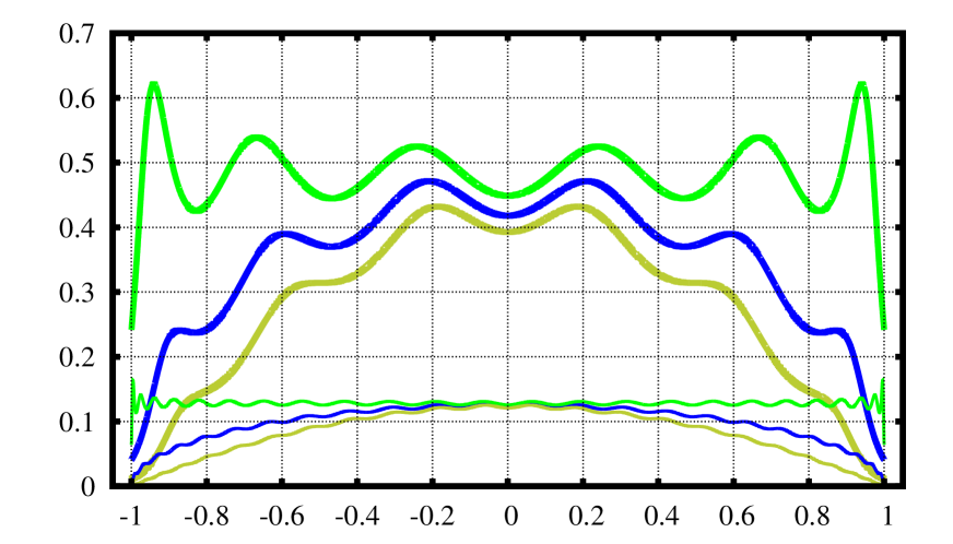
Figure 1: The Christoffel function $K(x)$ for the measures $d\mu=dx$ (blue), $d\mu=dx/\sqrt{1-x^{2}}$ (green), and $d\mu=dx\sqrt{1-x^{2}}$ (olive) with $n=7$ and $n=25$ (thin). The $1/K(x)$ is a polynomial on $x$ of the degree $2n-2$. Christoffel function is determined by integration measure and the basis used. If one chooses the harmonic basis: $\nicefrac{{1}}{{\sqrt{2}}}$,   $\sin(k\pi x)$, $\cos(k\pi x)$, $x\in[-1:1]$, $d\mu=dx$, $k=1,\dots,n-1$ then, in contradistinction to the blue line of this chart for $d\mu=dx$ in a polynomial basis, the Christoffel function is exactly the constant $1/(n-0.5)$. Christoffel function study for non–polynomial bases may be an important direction of further research. The first step in this direction is numerical experiments: from polynomial bases (where an extra degree gives one more basis function) to harmonic basis (where an extra degree gives two more basis functions), following a transition to ‘‘product’’ attributes (47), where the number of basis functions growths with a degree as (50).

In Fig. 1 a demonstration of the Christoffel function in 1D case is presented for the measures: $d\mu=dx$ and Chebyshev first and second kind $d\mu=dx/\sqrt{1-x^{2}}$ and $d\mu=dx\sqrt{1-x^{2}}$. One can see from the figure that $K(x)$ for Chebyshev measure $d\mu=dx/\sqrt{1-x^{2}}$ is close to a constant, this follows from the fact that all Gaussian quadrature weights are the same for Chebyshev measure. The operator $\|\rho_{K}\|$ allows us to construct a Chebyshev–like measure for a multi–dimensional basis:

$$\|\rho_{TK}\| =\sum\limits_{i=0}^{n-1}\Ket{\psi^{[i]}_{K}}\lambda_{TK}^{[i]}\Bra{\psi^{[i]}_{K}}$$ (39)

$$\lambda_{TK}^{[i]} =\frac{\Braket{1}}{n}$$ (40)

The operator $\|\rho_{TK}\|$ has the same eigenvectors as the $\|\rho_{K}\|$, but different eigenvalues; all the eigenvalues are now the same (40), this is a generalization from 1D Chebyshev measure. For a large enough $n$ density matrix operator (39) has similar to Chebyshev measure properties. Note that the entropy (38) is maximal for (40) distribution (all weights are equal). One may also consider to put entropy density $s(\mathbf{x})=-K(\mathbf{x})\ln\big{(}K(\mathbf{x})/\Braket{1}\big{)}$ to Eq. (34) instead of $K(\mathbf{x})$ from Eq. (10) to obtain a ‘‘spectral decomposition of the entropy’’ as $S=\sum\limits_{i=0}^{n-1}\lambda_{s}^{[i]}$. But it would be less convenient than the entropy (38), where we construct a discrete distribution $\lambda_{K}^{[i]}$ and the entropy is then calculated in a usual way. For a large enough $n$ these two approaches produce similar results.

The technique of an operator’s eigenvalues adjustment was originally developed in [14] and applied to hydroacoustic signals processing: first a covariation matrix is obtained and diagonalized, second the eigenvalues (not the eigenvectors!) are adjusted for an effective identification of weak hydroacoustic signals. The (39) is a transform of this type.

Before we go further let us take advantage of the basis $\Ket{\psi_{K}^{[i]}}$ uniqueness to obtain a familiar PCA variation expansion (16) but with the Christoffel function operator (36), the average is defined as matrix Spur:

$$\mathrm{Spur}\left(\|\rho_{K}\|-\frac{\Braket{1}}{n}\|1\|\right)^{2} =\sum\limits_{i=0}^{n-1}\left(\lambda^{[i]}_{K}-\frac{\Braket{1}}{n}\right)^{2}$$ (41)

The (41) is invariant with respect to an arbitrary non–degenerated linear transform of $\mathbf{x}$ components, no scaling and normalizing is required, same as for (16). One can select a few eigenvectors with a large $\lambda^{[i]}_{K}-\Braket{1}/n$ difference to capture ‘‘most of variation’’. However, our goal is not to capture ‘‘most of variation’’ but to construct a basis of the dimension $D\leq n$ that optimally separates the dataset. Note that when the $\|\rho_{TK}\|$ operator is used in (41) the variation is minimal (zero).

We are interested not in variance expansion, but in coverage expansion. If we sort eigenvalues in (37)

$$\Braket{1} =\sum\limits_{i=0}^{n-1}\lambda_{K}^{[i]}=\sum\limits_{i=0}^{n-1}\Braket{\psi_{K}^{[i]}}{\rho_{K}}{\psi_{K}^{[i]}}$$ (42)

is a sum of continuously decreasing terms, by selecting a few eigenvectors we can create a projected state, that covers a large portion of observations. This portion is minimal for Chebyshev density matrix (39), where it is equal to the ratio of the number of taken/total eigenvalues. As in the previous section we are going to obtain $D\leq n$ states that optimally separate the $\|\rho_{K}\|$ by constructing a Gaussian quadrature of the dimension $D$. However, in it’s original form there is an issue with the measure (26).

For $f(\mathbf{x})=K(\mathbf{x})$ a different separation criteria is required. Consider the measure ‘‘all eigenvalues are equal’’, a typical one used in random matrix theory, it is actually the Chebyshev density matrix (39).

$$\Braket{g(f)}_{E} =\sum\limits_{i=0}^{n-1}g(\lambda_{K}^{[i]})$$ (43)

$$\Braket{1}_{E} =n$$ (44)

The measure (43) takes all eigenvectors of (5) with equal weight, the nodes are $\lambda_{K}^{[i]}$, the weight is 1 for every node. If we now construct the Gaussian quadrature (28) on the measure $\Braket{\cdot}_{E}$ instead of the $\Braket{\cdot}_{L}$, the quadrature nodes

$$\lambda_{G}^{[m]} =\frac{\Braket{\psi_{G}^{[m]}}{f}{\psi_{G}^{[m]}}_{E}}{\Braket{\psi_{G}^{[m]}}{\psi_{G}^{[m]}}_{E}}=\frac{\sum\limits_{i=0}^{n-1}\lambda_{K}^{[i]}\left[\psi_{G}^{[m]}(\lambda_{K}^{[i]})\right]^{2}}{\sum\limits_{i=0}^{n-1}\left[\psi_{G}^{[m]}(\lambda_{K}^{[i]})\right]^{2}} m=0\dots D-1$$ (45)

have a meaning of a weight per original eigenvalue. Then $m=0\dots D-1$ eigenfunctions $\psi_{G}^{[m]}(f)$ of (28d) optimally cluster the weight per eigenvalue, a ‘‘density’’ like function required for unsupervised learning. The measure (43) does not allow to convert obtained optimal clustering solution $\psi_{G}^{[m]}(f)$, a pure state in $f$–space, to a pure state in $\mathbf{x}$–space $\psi_{G}^{[m]}(\mathbf{x})$, however it can be converted to a density matrix state $\|\Psi_{G}^{[m]}\|$, see Appendix C of [1]. While the $\psi_{G}^{[m]}(\mathbf{x})$ does not exist for a mixed state, the $p^{[m]}(\mathbf{x})$, an analogue of $\left[\psi_{G}^{[m]}(\mathbf{x})\right]^{2}$ that enters to the solutions of Radon–Nikodym type, can always be obtained. For the measure (43) the conversion is:

$$p^{[m]}(\mathbf{x}) =\sum\limits_{i=0}^{n-1}\left[\psi_{K}^{[i]}(\mathbf{x})\psi_{G}^{[m]}(\lambda_{K}^{[i]})\right]^{2} m=0\dots D-1$$ (46)

for a general case see Appendix C of [1].

In this section a completely new look to unsupervised learning PCA expansion is presented. Whereas a ‘‘regular’’ PCA expansion is attributes variation expansion, which is scale–dependent and often does not have a clear domain problem meaning, the Christoffel function density matrix expansion (42) is coverage expansion: every eigenvector covers some observations, total sum of the eigenvalues is equal to total measure $\Braket{1}$, the answer is invariant relatively any non–degenerated linear transform of input vector $\mathbf{x}$ components. In the simplistic form one can select a few eigenvectors with a large $\lambda_{K}^{[i]})$ (e.g. use --flag_replace_f_by_christoffel_function=true with the Appendix B software). In a more advanced form $D\leq n$ optimal clusters can be obtained by constructing a Gaussian quadrature with the measure (43) and then converting the result back to $\mathbf{x}$–space with (46) projections.

IV Selection of the Answer: $f_{RN}$ vs. $f_{RNW}$

For a given input attributes vector we now have two answers: interpolation $f_{RN}$ (13) and classification $f_{RNW}$ (18). Both are the answers of Radon–Nikodym $\Braket{f\psi^{2}}/\Braket{\psi^{2}}$ form, that can be reduced to weighted eigenvalues with $\mathrm{Proj}^{[i]}$ and $w^{[i]}\mathrm{Proj}^{[i]}$ weights respectively. A question arise which one to apply.

For a deterministic function $f(\mathbf{x})$, the $\mathrm{Proj}^{[i]}$ weights from (22) construct the state in $\Ket{\psi^{[i]}}$ basis that is the most close to a given observation $\mathbf{x}$. The $f_{RN}$ is a regular Radon–Nikodym derivative of the measures $fd\mu$ and $d\mu$, see Section II.C of [1]. This is a solution of interpolatory type, see Appendix C below for a demonstration.

For a probabilistic $f$ the $w^{[i]}\mathrm{Proj}^{[i]}$ weights, that include prior probability of $f$ outcomes, is a preferable form of outcome probabilities estimation, see Appendix B.2 below for a demonstration. The $w^{[i]}\mathrm{Proj}^{[i]}$ posterior weights typically produce a good classification even without optimal clustering algorithm of Section III. For a given scalar $f$ the solution to supervised learning problem is obtained in the form of (outcome,weight) posterior distribution (17b).

For unsupervised learning the function $f$ does not exist, thus the eigenvalue problem (4) cannot be formulated. However, we still want to obtain a unique basis that is constructed from the data, for example to avoid PCA dependence on attributes scale. For unsupervised learning the Christoffel function should be used as $f(\mathbf{x})=K(\mathbf{x})$, then PCA expansion of coverage can be obtained, this is an approach of Section III.1 to unsupervised learning.

V A First Order Logic Answer To The Classification Problem. Product Attributes.

Obtained solutions to interpolation (13) and classification (17b) problems are more general than a propositional logic type of answer. A regular basis function expansion (3) is a local function of arguments, thus it can be considered as a ‘‘propositional logic’’ type of answer. Consider formulas including a quantor operator, e.g. for a binary $x_{k}$ and $f$ in (1) expressions like these:

$$\mathrm{if}\,\exists x_{k}=1 f=1$$ then

$$\mathrm{if}\,\forall x_{k}=0 f=1$$ then

Similar expressions can be written for continuous $x_{k}$ and $f$, the difference from the propositional logic is that these expressions include a quantor–like operator that is a function of several $x_{k}$ attributes. The $\psi^{2}(\mathbf{x})$ expansion includes the products of $x_{j}x_{k}$, thus the Radon–Nikodym representation can be viewed as a more general form than a propositional logic. The most straightforward approach to obtain a ‘‘true’’ first order logic answer from a propositional logic model is to add all possible $Q_{k_{0}}(x_{0})Q_{k_{1}}(x_{1})\dots Q_{k_{n-1}}(x_{n-1})$ products to the list of input attributes. For a large enough ${\mathcal{D}}$ (49) we obtain a model with properties that are very similar to a first order logic model. The attributes $x_{\mathbf{k}}$ are now polynomials of $n$ variables with multi–index $\mathbf{k}$ of a degree ${\mathcal{D}}$; they are constructed from initial attributes $x_{k}$ with regular index $k$. Multi–index degree (49) is invariant relatively any linear transform of the attributes: $x^{\prime}_{j}=\sum_{k=0}^{n-1}T_{jk}x_{k}$. Because in the Radon–Nikodym approach all the answers are invariant relatively any non–degenerated linear transform of the basis, we can construct similar to the first order logic knowledge representation with known invariant group! The situation is different with logical formulas of disjunctive conjunction or conjunctive disjunction, where a basis transform change formula index[11], and the invariant group is either completely unknown or poorly understood; a typical solution in this situation is to introduce a ‘‘formula complexity’’ concept to limit the formulas to be considered, a mutli–index constraint (49) can be viewed as a complexity of the formulas allowed. The terms

$$x_{\mathbf{k}} =x_{0}^{k_{0}}x_{1}^{k_{1}}\dots x_{n-1}^{k_{n-1}}$$ (47)

$$\mathbf{k} =(k_{0},k_{1},\dots,k_{n-1})$$ (48)

$${\mathcal{D}} =\sum\limits_{j=0}^{n-1}k_{j}$$ (49)

$${\mathcal{N}}(n,{\mathcal{D}}) =C_{n+{\mathcal{D}}-1}^{\mathcal{D}}$$ (50)

are now identified by a multi–index $\mathbf{k}$ and added to (1) as attributes. We will call the set of all possible (47) terms used as ML attributes in (1) — the ‘‘product’’ attributes. An individual (47) is called ‘‘term’’, see [17, 18, 19]. The number ${\mathcal{N}}(n,{\mathcal{D}})$ of ‘‘product’’ attributes is the number of possible polynomial distinct terms with multi–index not higher than ${\mathcal{D}}$, it is equal to (50). A few values: ${\mathcal{N}}(n,1)=n$, ${\mathcal{N}}(n,2)=(n+1)n/2$, ${\mathcal{N}}(7,7)=1716$, ${\mathcal{N}}(8,7)=3432$, etc. In a typical ML setup such a transform to ‘‘product’’ attributes is not a good idea because of:

• A linear transform of input attributes produces a different solution, no gauge invariance.

• Attributes offset and normalizing difficulty.

• Data overfitting (curse of dimensionality), as we now have a much bigger number of input attributes ${\mathcal{N}}(n,{\mathcal{D}})$. A second complexity criteria (the first one is maximal multi–index (49)) of constructed attributes is typically introduced to limit the number of input attributes. For example, a neural network topology can be considered as a variant of a complexity criteria.

The approach developed in this paper has these difficulties solved. The invariant group is a non–degenerated linear transform $T_{jk}$ of input attributes components, the $x_{j}x_{k}$ and $\sum_{j^{\prime},k^{\prime}=0}^{n-1}T_{jj^{\prime}}x_{j^{\prime}}T_{kk^{\prime}}x_{k^{\prime}}$ attributes produce identical solutions; for the same reason the terms (47) $Q_{k_{0}}(x_{0})Q_{k_{1}}(x_{1})\dots Q_{k_{n-1}}(x_{n-1})$ are $Q_{k}$ invariant, e.g. $Q_{k}(x)=x^{k}$ and $Q_{k}(x)=T_{k}(x)$ produce identical solutions. The attributes offset and normalizing are not important since (5) is invariant relatively any non–degenerated linear transform of $\mathbf{x}$ components. The problem of data overfitting is not an issue since Section III optimal clustering solution (30) allows to reduce ${\mathcal{N}}(n,{\mathcal{D}})$ input attributes to a given number $D$ of their linear combinations that optimally separate the $f$. The only cost to pay is that the Lebesgue quadrature now requires a generalized eigenproblem of ${\mathcal{N}}(n,{\mathcal{D}})$ dimension to be solved, but this is purely a computational complexity issue. Critically important, that we are now limited not by the data overfitting, but by the computational complexity. Regardless input attributes number the optimal clustering solution (30) selects given number $D\ll{\mathcal{N}}(n,{\mathcal{D}})$ of input attributes linear combinations that optimally separate $f$ in terms of $\Braket{f\psi^{2}}/\Braket{\psi^{2}}$.

In the Appendix C a simple example of usage of polynomial function of a single attribute $x$ as input attributes was demonstrated (159). Similarly, a polynomial of several variables (47) identified by the multi–index (48) can be used to construct input attributes. An increase of attributes number from $n$ to ${\mathcal{N}}(n,{\mathcal{D}})$ using ‘‘product’’ attributes (47) combined with subsequent attributes number decrease to $D$ by the clustering solution (30) is a path to ML answers of the first order logic type: $n$ original attributes (1) $\rightarrow$ ${\mathcal{N}}(n,{\mathcal{D}})$ ‘‘product’’ attributes (47) $\rightarrow$ $D$ cluster attributes (30).

V.1 Lenna Image Interpolation Example. Multi–index Constraints Comparison.

In [20] a two–dimensional image interpolation problem was considered with multi–index $\mathbf{j}$ constraint

$$(x,y)^{(l)} \to f^{(l)} \omega^{(l)}=1$$ weight (51)

$$\mathbf{j} =(j_{x},j_{y})$$ (52)

$$0 \leq j_{x}\leq n_{x}-1$$ (53)

$$0 \leq j_{y}\leq n_{y}-1$$ (54)

basis $$:x^{j_{x}}y^{j_{y}} \dim(\text{basis})=n_{x}n_{y}$$ (55)

of each multi–index component being in the $[0\dots n_{\{x,y\}}-1]$ range; total number of basis functions is then $n_{x}n_{y}$ (55). This is different from the constraint (49), where the sum of all multi–index components is equal to ${\mathcal{D}}$; total number of basis functions is then (59). Different basis functions produce different interpolation, let us compare the interpolation in these two bases. Transform $d_{x}\times d_{y}$ image pixel coordinates $(x,y)$ ($x=0\dots d_{x}-1$; $y=0\dots d_{y}-1$) and gray intensity $f$ to the data of (1) form:

$$(x,y,1)^{(l)} \to f^{(l)} \omega^{(l)}=1$$ weight (56)

$$\mathbf{j} =(j_{x},j_{y},j_{c})$$ (57)

$${\mathcal{D}} =j_{x}+j_{y}+j_{c}$$ (58)

basis $$:x^{j_{x}}y^{j_{y}}=x^{j_{x}}y^{j_{y}}1^{j_{c}} \dim(\text{basis})={\mathcal{N}}(n,{\mathcal{D}})$$ (59)

Input attributes vector $\mathbf{x}$ is of the dimension $n=3$: two pixel coordinates and const, this way the (47) ‘‘product’’ attributes with the constraint (58) include all $x^{j_{x}}y^{j_{y}}$ terms with lower than ${\mathcal{D}}$ degree $j_{x}+j_{y}\leq{\mathcal{D}}$. Observation index $l$ runs from $1$ to the total number of pixels $M=d_{x}\times d_{y}$.

Let us compare [20] $n_{x}=n_{y}=50;\dim(\text{basis})=n_{x}n_{y}=2500$ of basis (55) with $n=3;{\mathcal{D}}=69;\dim(\text{basis})={\mathcal{N}}(n,{\mathcal{D}})=2485$ of basis (59). The value of ${\mathcal{D}}=69$ is selected to have approximately the same total number of basis functions. The bases are different: $x^{67}y^{2}$, $x^{66}y^{2}$, etc. are among ‘‘product’’ attributes (59), but they are not among the (55) where the maximal degree for $x$ and $y$ is $49$; similarly the $x^{49}y^{49}$ is in (55), but it is not in (59). As in [20] we choose 512x512 Lenna grayscale image as a testbed. If you have scala installed run

 scala com.polytechnik.algorithms.ExampleImageInterpolation \
   file:dataexamples/lena512.bmp 50 50 chebyshev

to reproduce [20] results using (8) and (9) for least squares and Radon–Nikodym. Then run (note: this code is unoptimized and slow):

 java com/polytechnik/algorithms/ExampleImageInterpolation2 \
   file:dataexamples/lena512.bmp 50 50 69

To obtain 4 files. The files lena512.bmp.LS.50.50.bs2500.png and lena512.bmp.RN.50.50.bs2500.png are obtained as (12) and (13) using (55) basis with $n_{x}=n_{y}=50$, the result is identical to [20]. The files lena512.bmp.LS.D.69.bs2485.png and lena512.bmp.RN.D.69.bs2485.png are obtained from (12) and (13) using (59) basis with ${\mathcal{D}}=69$. The images are presented in Fig. 2.

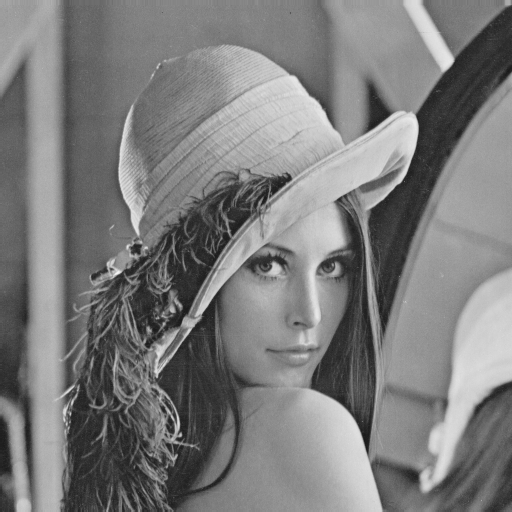
Figure 2: Top: original image. Middle: least squares in (55) basis (left) and (59) basis (right). Bottom: Radon–Nikodym in (55) basis (left) and (59) basis (right). The bases (55) and (59) are of 2500 elements ($n_{x}=n_{y}=50$) and 2485 elements ($n=3$, ${\mathcal{D}}=69$) respectively.

It was shown in [20] that the Radon–Nikodym interpolation produces a sfumato type of picture because it averages with always positive weight $\psi^{2}(\mathbf{x})$; the (13) preserves the bounds of $f$: if original gray intensity is $[0:1]$ bounded then interpolated gray intensity is $[0:1]$ bounded as well; this is an important difference from positive polynomials interpolation[21] where only a low bound (zero) is preserved. In contradistinction to Radon–Nikodym the least squares interpolation strongly oscillates near image edges and may not preserve the bounds of gray intensity $f$. In this section we compare not least squares vs. Radon–Nikodym as we did in [20] but the bases: (55) vs. (59) as they have different multi–index constraints. We observe that:

• The bases produce similar results. Basis differences in LS are more pronounced, than in RN; always positive weight makes the RN less sensitive to basis choice.

• In RN a small difference is observed near image edges. With (55) RN still has small oscillations near edges, and with (59) RN has oscillations completely suppressed.

• The multi–index constraint (55) is not invariant relatively a linear transform of input attributes, for example $x^{n_{x}-1}y^{n_{y}-1}$ relatively $x=x^{\prime}-y^{\prime}$, $y=x^{\prime}+y^{\prime}$, but the (59) is invariant.

This make us to conclude that the specific multi–index constraint is not very important, the results are similar. Whereas in an interpolation problem an explosion of basis functions number increases interpolation precision, in a classification problem an explosion of basis functions number leads to data overfitting. The optimal clustering solution (30) reduces the number of basis functions to a given $D$ thus it solves the problem of data overfitting. This reduction makes multi–index constraint used for initial basis construction even less important for a classification problem than for an interpolation problem.

V.2 On The Christoffel Function Conditional Optimization

All the solutions obtained in this paper have a distribution of $f$ as the answer: the distribution with posterior weights (17b), optimal clustering (28), etc. Recently, a promising approach to interpolation problem has been developed [22]. In this subsection we consider a modification of it to obtain, for a given $\mathbf{x}$, not a single outcome of $f$, but a distribution. Obtained weights can be considered as an alternative to the posterior weights (17b). A sketch of [22] theory:

• Introduce a vector $\mathbf{z}=(\mathbf{x},f)$ of the dimension $n+1$.

• Construct ‘‘product’’ attributes (47) out of $\mathbf{z}$ components with the degree equals to ${\mathcal{D}}$; because a constant always presents in $x_{k}$ it is sufficient to consider the degree equals to ${\mathcal{D}}$, lower order terms are obtained automatically as in (59). There are ${\mathcal{N}}(n+1,{\mathcal{D}})$ ‘‘product’’ attributes obtained from $n+1$ components of $\mathbf{z}$.

• Construct Christoffel function (10) from obtained ‘‘product’’ attributes $K(\mathbf{z})=K(\mathbf{x},f)$. Now the $1/K(\mathbf{z})$, for a given $\mathbf{x}$, is a positive polynomial on $f$ of the degree $2{\mathcal{D}}$.

• For a given $\mathbf{x}$, the interpolation [22] of $f$ is the value providing the minimum of the polynomial $1/K(\mathbf{x},f)$; the value of $\mathbf{x}$ is fixed:

  $$K(\mathbf{x},f)\Big{|}_{\mathbf{x}} \xrightarrow[f]{\quad}\max$$ (60)

As an extension of this approach consider Christoffel function average, Appendix B of [1], but use the $K(\mathbf{z})=K(\mathbf{x},f)$ to calculate the moments of $f$:

$$\Braket{f^{m}}_{K(\mathbf{x},\cdot)} =\Braket{f^{m}K(\mathbf{z})\Big{missing}}{{}_{\mathbf{x}}}=\sum\limits_{l=1}^{M}\frac{\left(f^{(l)}\right)^{m}}{1/K(\mathbf{x},f^{(l)})}\omega^{(l)}$$ (61)

When one uses $\mathbf{x}=\mathbf{x}^{(l)}$ as Christoffel function argument in the right hand side of (61), the average is the Christoffel function average of Ref. [1] with the properties similar to regular average (7); the Gaussian quadrature built from the moments obtained with the Christoffel function average is similar to the one built from the regular moments $\Braket{f^{m}}$, and to the one built from (26) moments with $g=f^{m}$. However, if to consider a fixed value of $\mathbf{x}$, then the solution becomes similar to the approach of Ref. [22], the $K(\mathbf{x},f)$ is now used as a proxy to joint distribution $\rho(\mathbf{x},f)$. Because $1/K(\mathbf{x},f)$ at fixed $\mathbf{x}$ is a positive polynomial on $f$ of the degree $2{\mathcal{D}}$, the moments $\Braket{f^{m}}_{K(\mathbf{x},\cdot)}$ do exist for at least $m=0\dots 2{\mathcal{D}}$. A ${\mathcal{D}}$–point Gaussian quadrature can be built from them, exactly as (28), but with the measure $\Braket{\cdot}_{K(\mathbf{x},\cdot)}$ instead of $\Braket{\cdot}_{L}$. The result is ${\mathcal{D}}$ nodes (28f) and weights (28g). The major difference from [22] is that instead of single $f$ we now obtained $i=0\dots\mathcal{D}-1$ (outcome,weight) pairs $(f_{K(\mathbf{x},\cdot)}^{[i]},w_{K(\mathbf{x},\cdot)}^{[i]})$ of the distribution of $f$ conditional to a given $\mathbf{x}$. The most close to [22] interpolation answer is to find the $f_{K(\mathbf{x},\cdot)}^{[i]}$, corresponding to the maximal $w_{K(\mathbf{x},\cdot)}^{[i]}$. However, in ML the distribution of outcomes, not a single ‘‘answer’’, is of most interest. From the Gaussian quadrature built on the $\Braket{\cdot}_{K(\mathbf{x},\cdot)}$ measure conditional distribution characteristics can be obtained:

• The $\Braket{1}_{K(\mathbf{x},\cdot)}$ is an analogue of $\mathrm{Coverage}(\mathbf{x})$ from (19): how many observations are ‘‘close enough’’ to a given $\mathbf{x}$.

• The Gaussian quadrature nodes and weights $(f_{K(\mathbf{x},\cdot)}^{[i]},w_{K(\mathbf{x},\cdot)}^{[i]})$ are an analogue of the posterior distribution (17b). However, in (61) approach both: the outcomes $f_{K(\mathbf{x},\cdot)}^{[i]}$ and the weights $w_{K(\mathbf{x},\cdot)}^{[i]}$ depend on $\mathbf{x}$. In (17b) approach the outcomes are always the same $f^{[i]}$ and only posterior weights depend on $\mathbf{x}$ as $w^{[i]}\mathrm{Proj}^{[i]}(\mathbf{x})$. This distinction is similar to [3] with $\mathbf{x}$–dependent outcomes vs. [23] with $\mathbf{x}$–independent outcomes.

• The approach (61) cannot provide an optimal clustering solution of (30) type. Ideologically, $\mathbf{x}$–dependent outcomes make optimal clustering difficult. Technically, the $m=0\dots 2{\mathcal{D}}$ moments $\Braket{f^{m}}_{K(\mathbf{x},\cdot)}$ cannot be reduced to a density matrix average of Appendix C of [1] or to a simple pure state average (15b).

VI A Supervised Classification Problem With Vector–Valued Class Label

In the ML problem (1) the class label $f$ is considered to be a scalar. A problem with vector–valued class label $\mathbf{f}$

$$(x_{0},x_{1},\dots,x_{k},\dots,x_{n-1})^{(l)} \to(f_{0},f_{1},\dots,f_{j},\dots,f_{m-1})^{(l)} \omega^{(l)}$$ weight (62)

where an attributes vector $\mathbf{x}$ of the dimension $n$ is mapped to a class label vector $\mathbf{f}$ of the dimension $m$ is a much more interesting case. For a vector class label $\mathbf{f}$, the most straightforward approach is to build an individual model for every $f_{j}$ component. However, constructed models are often completely different and obtained model set cannot be viewed as a probability space. In addition, the invariant group of $\mathbf{f}$ (what transform of $f_{j}$ components does not change the prediction) may become unknown and basis–dependent. The situation is similar to the one of our previous works[3, 23], where the distribution regression problem can be directly approached by the Radon–Nikodym technique, however the distribution to distribution regression problem is a much more difficult case.

Whereas the Christoffel function maximization approach (60) of Ref. [22] is interesting for a scalar $f$, it becomes extremely promising for a vector class label $\mathbf{f}$. Consider a vector $\mathbf{z}$ of the dimension $n+m$:

$$\mathbf{z} =(x_{0},x_{1},\dots,x_{k},\dots,x_{n-1},f_{0},f_{1},\dots,f_{j},\dots,f_{m-1})^{(l)} \omega^{(l)}$$ weight (63)

The vector $\mathbf{z}$ mixes input attributes $\mathbf{x}$ with class label vector $\mathbf{f}$. The ${\mathcal{N}}(n+m,{\mathcal{D}})$ ‘‘product’’ attributes $Z_{i}$ can be obtained out of $n+m$ $\mathbf{z}$ components as in (47). The ‘‘product’’ attributes $Z_{i}$ with the constraint (49) are the ones with the simplest invariant group: the answer is invariant relatively any non–degenerated linear transform of $\mathbf{z}$ components: $z^{\prime}_{s}=\sum_{s^{\prime}=0}^{n+m-1}T_{ss^{\prime}}z_{s^{\prime}}$; $s,s^{\prime}=0\dots n+m-1$. The invariant group can be viewed as a gauge transformations and is a critical insight into the ML model built.

From (63) $\mathbf{z}$ data construct ${\mathcal{N}}(n+m,{\mathcal{D}})$ ‘‘product’’ attributes $Z_{i}$ according to (49) (if necessary perform regularization of the Appendix A), then, finally, construct the Christoffel function $K(\mathbf{z})$ according to (10). Classification problem is to find $\mathbf{f}$–prediction for a given $\mathbf{x}$. When one puts $x_{k},k=0\dots n-1$ part of vector $\mathbf{z}$ equal to a given $\mathbf{x}$ the $K(\mathbf{x},\mathbf{f})$, for a fixed $\mathbf{x}$, can be viewed as a a proxy to joint distribution $\rho(\mathbf{x},\mathbf{f})$. Find it’s maximum over the vector $\mathbf{f}$:

$$K(\mathbf{x},\mathbf{f})\Big{|}_{\mathbf{x}} \xrightarrow[\mathbf{f}]{\quad}\max$$ (64)

to obtain Ref. [22] solution. The solution (64) is exactly (60), but with a vector class label $\mathbf{f}$!

For a fixed $\mathbf{x}$ and a degree ${\mathcal{D}}$ the $1/K(\mathbf{x},\mathbf{f})\Big{|}_{\mathbf{x}}$ is a polynomial on $f_{j}$ of the degree $2{\mathcal{D}}$, there are total ${\mathcal{N}}(m,{\mathcal{D}})$ distinct terms. In applications it may be convenient to minimize the polynomial $1/K(\mathbf{x},\mathbf{f})\Big{|}_{\mathbf{x}}$ instead of maximizing the Christoffel function (64), but these are implementation details.

Critically important, that, for a given $\mathbf{x}$, we now obtained a probability distribution of $\mathbf{f}$ as $K(\mathbf{x},\mathbf{f})\Big{|}_{\mathbf{x}}$. When a specific value of $\mathbf{f}$ is required, it can be estimated from the distribution as:

• Christoffel function maximum (64).

• The distribution of Christoffel function eigenvalues (34)

• The simplest one is to average $\mathbf{f}$ with $K(\mathbf{x},\mathbf{f})\Big{|}_{\mathbf{x}}$, same as (61) but with the vector $\mathbf{f}$ instead of $f^{m}$: $\Braket{\mathbf{f}K(\mathbf{z})\Big{missing}}{{}_{\mathbf{x}}}$ and similar generalizations.

The most remarkable feature is that the $K(\mathbf{x},\mathbf{f})\Big{|}_{\mathbf{x}}$ approach is trivially applicable to a vector class label $\mathbf{f}$, and the constructed model has a known ‘‘gauge group’’.

VI.1 A Vector–Valued Class Label: Selecting Solution Type

While the idea [22] to combine input attributes $\mathbf{x}$ with class label vector $\mathbf{f}$ into a single vector $\mathbf{z}$ (63) with subsequent construction of ‘‘product’’ attributes $\mathbf{Z}$ (47) and finally to obtain Gram matrix $\Braket{Z_{i}Z_{j}}$ and Christoffel function $K(\mathbf{z})$ (10) is a very promising one, it still has some limitations.

Consider a ${\mathcal{D}}=1$ example: let a datasample (62) has $f_{0}=x_{0}$ for all $l=1\dots M$. Then Gram matrix $\Braket{z_{i}z_{j}}$ is degenerated. When attributes regularization is applied — it will remove either $f_{0}$ or $x_{0}$ from $\mathbf{z}$, thus the resulting $K(\mathbf{z})\Big{|}_{\mathbf{x}}$ depends on attributes regularization: a polynomial $1/K(\mathbf{z})\Big{|}_{\mathbf{x}}$ on $\mathbf{f}$ is different, thus $\Braket{\mathbf{f}K(\mathbf{z})\Big{missing}}{{}_{\mathbf{x}}}$ produces the result depending on the regularization. An ultimate example of this situation is: for $k=0\dots n-1$, let $f_{k}=x_{k}$ for all $l=1\dots M$ with $n=m$. In this case Gram matrix has two copies of exactly the same attributes and what combination of them propagate to the final set of attributes depends on regularization. For example if $x_{k}$ are selected and $f_{k}$ are dropped then $K(\mathbf{z})\Big{|}_{\mathbf{x}}$ is a constant and $\Braket{\mathbf{f}K(\mathbf{z})\Big{missing}}{{}_{\mathbf{x}}}$ is $\mathbf{x}$–independent. Such a regularization–dependent answer cannot be a solid foundation to ML classification problem, a regularization–independent solution is required.

Consider two Gram matrices $\Braket{x_{k}x_{k^{\prime}}}$ and $\Braket{f_{j}f_{j^{\prime}}}$ with attributes possibly ‘‘producted’’ (47) to ${\mathcal{D}}_{x}$ and ${\mathcal{D}}_{f}$. It’s ‘‘gauge transformation’’ is:

$$x^{\prime}_{k} =\sum\limits_{k^{\prime}=0}^{n-1}T_{kk^{\prime}}x_{k^{\prime}}$$ (65a)

$$f^{\prime}_{j} =\sum\limits_{j^{\prime}=0}^{m-1}T_{jj^{\prime}}f_{j^{\prime}}$$ (65b)

There are no $\mathbf{x}\Leftrightarrow\mathbf{z}$ ‘‘cross’’ terms as when we were working with the combined $\mathbf{z}$, this makes the solution regularization–independent.

Consider the simplest practical solution. Let $x_{k}$ attributes being regularized and ‘‘producted’’ (47) to a degree ${\mathcal{D}}$. The $\mathbf{f}$ attributes are untransformed. The Radon–Nikodym interpolation solution (9) is directly applicable:

$$\mathbf{f}_{RN}(\mathbf{x}) =\frac{\sum\limits_{l,j,k,i=0}^{n-1}x_{l}G^{-1}_{lj}\Braket{x_{j}}{\mathbf{f}}{x_{k}}G^{-1}_{ki}x_{i}}{\sum\limits_{j,k=0}^{n-1}x_{j}G^{-1}_{jk}x_{k}}$$ (66)

This ‘‘vector’’ type of solution to distribution to distribution regression problem (that was obtained back in [23]) is just (9) applied to every component of $\mathbf{f}$. As we discussed in Section II and demonstrated in the Appendix B.2, such a solution, while being a good one to an interpolation problem, leads to data overfitting when applied to a classification problem. We need to use the posterior (17b) distribution weights to obtain an analogue of $f_{RNW}(\mathbf{x})$ (18), but without generalized eigenvalue problem on $f$, as the $\mathbf{f}$ is now a vector. This is feasible if we go from ‘‘regular’’ average to Christoffel function average of Section III.1. All density matrix averages posses the duality property[1]:

$$\mathrm{Spur}\,\|f|\rho_{K}\| =\sum\limits_{i=0}^{n-1}\lambda^{[i]}_{K}\Braket{\psi^{[i]}_{K}}{f}{\psi^{[i]}_{K}}=\sum\limits_{i=0}^{n-1}\lambda^{[i]}_{f}\Braket{\psi^{[i]}_{f}}{\rho_{K}}{\psi^{[i]}_{f}}$$ (67)

Thus, for a vector $\mathbf{f}$, where the pairs $\left(\lambda^{[i]}_{f};\Ket{\psi^{[i]}_{f}}\right)$ do not exist, obtain in $\Ket{\psi^{[i]}_{K}}$ basis:

$$\mathbf{f}_{RNW}(\mathbf{x}) =\frac{\sum\limits_{i=0}^{n-1}\lambda^{[i]}_{K}\left[\psi^{[i]}_{K}(\mathbf{x})\right]^{2}\Braket{\psi^{[i]}_{K}}{\mathbf{f}}{\psi^{[i]}_{K}}}{\sum\limits_{i=0}^{n-1}\lambda^{[i]}_{K}\left[\psi^{[i]}_{K}(\mathbf{x})\right]^{2}}$$ (68)

This is the simplest practical solution to a classification problem with vector class label $\mathbf{f}$. It uses unsupervised learning basis $\Ket{\psi^{[i]}_{K}}$ of generalized eigenvalue problem (34) to solve the problem with a vector class label $\mathbf{f}$. The solution (68) assumes every component of vector $\mathbf{f}$ is diagonal in the basis $\Ket{\psi_{K}^{[i]}}$. This is not generally the case, but allows to build a single classificator for a vector class label $\mathbf{f}$ instead of constructing an individual classificator for every $f_{j}$ component. The option --flag_assume_f_is_diagonal_in_christoffel_function_basis=true of the provided software (see Appendix B below) builds such a classifier. This ‘‘same $\Ket{\psi_{K}^{[i]}}$ basis for all $f_{j}$’’ classifier typically has worse quality that the one built in $\Ket{\psi^{[i]}}$ basis corresponding to an individual scalar class label $f_{j}$

The approach of two Gram matrices $\Braket{x_{k}x_{k^{\prime}}}$, $k,k^{\prime}=0\dots n-1$ and $\Braket{f_{j}f_{j^{\prime}}}$, $j,j^{\prime}=0\dots m-1$ without ‘‘mixed’’ terms $\Braket{x_{k}f_{j}}$ in basis allows to obtain a ‘‘relative frequency’’ characteristic, a density of state type of solution. Consider ${\mathcal{R}}$, the ratio of two Christoffel functions:

$$K(\mathbf{f}(\mathbf{x})) ={\mathcal{R}}\cdot K(\mathbf{x})$$ (69)

$${\mathcal{R}} =\frac{\sum\limits_{k,k^{\prime}=0}^{n-1}\alpha_{k}\Braket{x_{k}}{K(\mathbf{f(\mathbf{x})})}{x_{k^{\prime}}}\alpha_{k^{\prime}}}{\sum\limits_{k,k^{\prime}=0}^{n-1}\alpha_{k}\Braket{x_{k}}{K(\mathbf{x})}{x_{k^{\prime}}}\alpha_{k^{\prime}}}$$ (70)

which is an estimator of Radon–Nikodym derivative[25]. The ${\mathcal{R}}$ is a dimensionless ‘‘relative frequency’’: how often a given realization of vector $\mathbf{f}$ corresponds to a given realization of vector $\mathbf{x}$ in (62) sample. The $K(\mathbf{x})$ and $K(\mathbf{f})$ are Christoffel functions calculated on $\mathbf{x}$ and $\mathbf{f}$ portion of (62) data, possibly regularized and ‘‘producted’’. The $1/K(\mathbf{x})$ and $1/K(\mathbf{f})$ are positive polynomials on $x_{k}$ and $f_{j}$ components respectively.

To obtain the distribution of ${\mathcal{R}}$ multiply left- and right- hand side of (69) by $\psi^{2}(\mathbf{x})$ and integrate it over all $l=1\dots M$ observations of (62) datasample, obtain (70). The calculation of $\Braket{x_{k}}{K(\mathbf{f(\mathbf{x})})}{x_{k^{\prime}}}$ matrix elements is no different from the one performed in (34): use (10) expression, but now in $\mathbf{f}$–space. A familiar generalized eigenvalue problem is then:

$$\sum\limits_{k^{\prime}=0}^{n-1}\Braket{x_{k}}{K(\mathbf{f(\mathbf{x})})}{x_{k^{\prime}}}\alpha^{[i]}_{k^{\prime}} =\lambda_{\mathcal{R}}^{[i]}\sum\limits_{k^{\prime}=0}^{n-1}\Braket{x_{k}}{K(\mathbf{x})}{x_{k^{\prime}}}\alpha^{[i]}_{k^{\prime}}$$ (71)

$$\psi_{\mathcal{R}}^{[i]}(\mathbf{x}) =\sum\limits_{k=0}^{n-1}\alpha^{[i]}_{k}x_{k}$$ (72)

Obtained $\lambda_{\mathcal{R}}^{[i]}$ is a spectrum of ‘‘relative frequency’’. In $\Ket{\psi_{\mathcal{R}}^{[i]}}$ state there are $\lambda_{\mathcal{R}}^{[i]}$ time more $\mathbf{f}$ observations than $\mathbf{x}$ observations. The matrices $\Braket{x_{k}}{K(\mathbf{f(\mathbf{x})})}{x_{k^{\prime}}}$ and $\Braket{x_{k}}{K(\mathbf{x})}{x_{k^{\prime}}}$ are $n\times n$ matrices calculated from a training datasample. The knowledge is accumulated in their spectrum. When evaluating a testing dataset the simplest usage of (70) is this: for a given $\mathbf{x}$, how often/seldom we see an $\mathbf{f}$? The answer is (70) with localized $\alpha_{k}=\sum_{k^{\prime}=0}^{n-1}G^{-1}_{kk^{\prime}}x_{k^{\prime}}$ or, when written in (72) basis

$${\mathcal{R}}(\mathbf{x}) =\frac{\sum\limits_{i=0}^{n-1}\lambda_{\mathcal{R}}^{[i]}\left[\psi_{\mathcal{R}}^{[i]}(\mathbf{x})\right]^{2}}{\sum\limits_{i=0}^{n-1}\left[\psi_{\mathcal{R}}^{[i]}(\mathbf{x})\right]^{2}}$$ (73)

While the (68) is $\mathbf{f}$–value predictor, the ${\mathcal{R}}$ is ‘‘relative frequency’’ estimator, an important characteristic when considering a vector–to–vector type of mapping.

VI.2 A Vector–Valued Class Label: Error Estimation

The vector–value estimators (66) and (68) are an estimation of $\mathbf{f}$ by averaging class label $\mathbf{f}^{(l)}=(f_{0},f_{1},\dots,f_{j},\dots,f_{m-1})^{(l)}$ from (63) with a $\mathbf{x}$– dependent positive weight $W_{\mathbf{x}}(\mathbf{x}^{(l)})$:

$$\mathbf{f}(\mathbf{x}) =\frac{\sum\limits_{l=1}^{M}W_{\mathbf{x}}(\mathbf{x}^{(l)})\mathbf{f}^{(l)}}{\sum\limits_{l=1}^{M}W_{\mathbf{x}}(\mathbf{x}^{(l)})}$$ (74)

$$\Braket{1}_{W_{\mathbf{x}}} =\sum\limits_{l=1}^{M}W_{\mathbf{x}}(\mathbf{x}^{(l)})$$ (75)

What is the best way to estimate an error of a solution of this type? A ‘‘traditional’’ approach would be to consider a standard deviation type of answer $\Braket{\left(f-\overline{f}\right)^{2}}$, a variation of $\mathbf{f}$ components relatively their average value. This solution can be obtained from Gram matrix in $\mathbf{f}$–space (with some complications because of vector class label $\mathbf{f}$):

$$G_{jk} =\Braket{f_{j}f_{k}}_{W_{\mathbf{x}}}=\sum\limits_{l=1}^{M}W_{\mathbf{x}}(\mathbf{x}^{(l)})f^{(l)}_{j}f^{(l)}_{k} j,k=0\dots m-1$$ (76)

As we discussed in [8] and then earlier in this paper all standard deviation error estimators cannot be applied to non–Gaussian data, thus they have a limited applicability domain. A much better estimator can be constructed from the Christoffel function. Consider Christoffel function in $\mathbf{f}$–space $K_{W_{\mathbf{x}}}(\mathbf{f})$, obtained from Gram matrix (76) as $1/K_{W_{\mathbf{x}}}(\mathbf{f})={\sum_{j,k=0}^{m-1}f_{j}G^{-1}_{jk}f_{k}}$, exactly as we did in (10) in $\mathbf{x}$–space. Consider the best possible situation when (74) has no variation, i.e. the averaging gives exact values. The support of this measure is then a single point $\mathbf{f}$ from (74) (compare with a Gaussian quadrature in case when a single node has a dominantly large weight). When a prediction is not perfect we have a variation of $\mathbf{f}^{(l)}$ around average. Exactly as we did above, instead of considering a variation in $\mathbf{f}$–space, consider the support of a measure, a ‘‘Lebesgue’’ style approach. The total measure is $\Braket{1}_{W_{\mathbf{x}}}$, the support of $\mathbf{f}$–localized state is $K_{W_{\mathbf{x}}}(\mathbf{f})$, their difference gives error estimation:

$$\mathrm{Error} =\Braket{1}_{W_{\mathbf{x}}}-K_{W_{\mathbf{x}}}(\mathbf{f})$$ (77)

$$\mathrm{Error}_{rel} =\frac{\mathrm{Error}}{\Braket{1}_{W_{\mathbf{x}}}}=1-\frac{K_{W_{\mathbf{x}}}(\mathbf{f})}{\Braket{1}_{W_{\mathbf{x}}}}$$ (78)

Error estimator (77) has a dimension of weight (number of observations). It has the meaning of the difference between total measure and the measure of $\mathbf{f}$–localized state. It is gauge invariant relatively (65).

Even when a predictor (in a form of $\mathbf{x}$– dependent positive weight $W_{\mathbf{x}}(\mathbf{x})$) does not exist we can still obtain an information of how well a vector in $\mathbf{f}$-space can be recovered from $\mathbf{x}$-space. In scalar case $\mathbf{f}=f$ the simplistic solution to the problem is the aforementioned $L^{2}$ norm (2): if standard deviation is zero then $f$ can be completely recovered from the value of $\mathbf{x}$. However, this solution, besides depending on the scale of $f$, is problematically to generalize to a vector $\mathbf{f}$.

We can construct an original solution to vector $\mathbf{f}$ from three matrices: $\Braket{f_{j^{\prime}}f_{k^{\prime}}}$ (the (76) with $W_{\mathbf{x}}=1$), $\Braket{x_{j}x_{k}}$, and $\Braket{x_{j}f_{k^{\prime}}}$. The first two are Gram matrices in $\mathbf{f}$- and $\mathbf{x}$- space respectively:

$$G^{\mathbf{f}}_{j^{\prime}k^{\prime}} =\Braket{f_{j^{\prime}}f_{k^{\prime}}} j^{\prime},k^{\prime}=0\dots m-1$$ (79)

$$G^{\mathbf{x}}_{jk} =\Braket{x_{j}x_{k}} j,k=0\dots n-1$$ (80)

$$G^{\mathbf{x}\mathbf{f}}_{jk^{\prime}} =\Braket{x_{j}f_{k^{\prime}}} j=0\dots n-1;k^{\prime}=0\dots m-1$$ (81)

In scalar $f$ case we have $m=2$ or greater:

$$\mathbf{f} =(1,f) f_{0}=1;f_{1}=f;m=2$$ (82)

$$\mathbf{f} =(1,f,f^{2}) f_{0}=1;f_{1}=f;f_{2}=f^{2};m=3$$

$$\mathbf{f} =(1,f,f^{2},f^{3}) f_{0}=1;f_{1}=f;f_{1}=f^{2};f_{3}=f^{3};m=4$$

a constant should always present in the basis (both in $\mathbf{f}$ and $\mathbf{x}$). A criterion of how well $\mathbf{f}$ can be recovered from $\mathbf{x}$ is to compare the matrices $\Braket{f_{j^{\prime}}f_{k^{\prime}}}$ and $\Braket{f_{j^{\prime}}(\mathbf{x})f_{k^{\prime}}(\mathbf{x})}$; the $f_{j^{\prime}}$ is exact value and the $f_{j^{\prime}}(\mathbf{x})$ is obtained from (8) projection of $\mathbf{f}$ on $\mathbf{x}$-space:

$$\mathbf{f}(\mathbf{x}) =\mathrm{Proj}^{(\mathbf{f\to x})}\mathbf{f}$$ (83)

$$f_{j^{\prime}}(\mathbf{x}) =\sum\limits_{j,k=0}^{n-1}x_{j}G^{\mathbf{x};\,-1}_{jk}\Braket{f_{j^{\prime}}x_{k}}$$ (84)

$$\Braket{f_{j^{\prime}}(\mathbf{x})f_{k^{\prime}}(\mathbf{x})} =\sum\limits_{j,k=0}^{n-1}\Braket{f_{j^{\prime}}x_{j}}G^{\mathbf{x};\,-1}_{jk}\Braket{f_{k^{\prime}}x_{k}}=\sum\limits_{j,k=0}^{n-1}G^{\mathbf{x}\mathbf{f}}_{jj^{\prime}}G^{\mathbf{x};\,-1}_{jk}G^{\mathbf{x}\mathbf{f}}_{kk^{\prime}}$$ (85)

Here $G^{\mathbf{x};\,-1}_{jk}$ is an inverse of $G^{\mathbf{x}}_{jk}$ from (80). The non–negative $m\times m$ symmetric matrices: $\Braket{f_{j^{\prime}}(\mathbf{x})f_{k^{\prime}}(\mathbf{x})}$ (Eq. (85)) and $\Braket{f_{j^{\prime}}f_{k^{\prime}}}$ (Eq. (79)) coincide if $\mathbf{f}$ is a subspace of $\mathbf{x}$; both represent the $\mathbf{f}$-space: the former is projected on $\mathbf{x}$, the later is calculated directly.

Solve generalized eigenproblem with these two matrices in left- and right- hand side respectively, exactly as in (5):

$$\sum\limits_{k^{\prime}=0}^{m-1}\Braket{f_{j^{\prime}}(\mathbf{x})f_{k^{\prime}}(\mathbf{x})}\alpha^{[i]}_{k^{\prime}} =\lambda^{[i]}\sum\limits_{k^{\prime}=0}^{m-1}\Braket{f_{j^{\prime}}}{f_{k^{\prime}}}\alpha^{[i]}_{k^{\prime}}$$ (86)

$$\sum\limits_{k^{\prime}=0}^{m-1}\sum\limits_{j,k=0}^{n-1}G^{\mathbf{x}\mathbf{f}}_{jj^{\prime}}G^{\mathbf{x};\,-1}_{jk}G^{\mathbf{x}\mathbf{f}}_{kk^{\prime}}\alpha^{[i]}_{k^{\prime}} =\lambda^{[i]}\sum\limits_{k^{\prime}=0}^{m-1}G^{\mathbf{f}}_{j^{\prime}k^{\prime}}\alpha^{[i]}_{k^{\prime}}$$

If $\mathbf{f}$-space is a subspace of $\mathbf{x}$-space then all $i=0\dots m-1$ eigenvalues $\lambda^{[i]}$ are equal to $1$ and their sum is equal to matrix $\Braket{f_{j^{\prime}}}{f_{k^{\prime}}}$ rank $m$. Otherwise the difference represents an error: how big is the remaining error after projecting $\mathbf{f}$-space on $\mathbf{x}$-space:

$$\mathrm{Error}_{rank} =m-\sum\limits_{i=0}^{m-1}\lambda^{[i]}=m-\sum\limits_{j,k=0}^{m-1}\Braket{f_{j}(\mathbf{x})f_{k}(\mathbf{x})}G^{\mathbf{f};\,-1}_{kj}$$ (87)

This error is gauge–invariant relatively (65), it is dimensionless and represents how well $\mathbf{f}$-space can be projected on $\mathbf{x}$-space. It can be viewed as a gauge–invariant ‘‘squared multi–dimensional correlation’’ between $\mathbf{f}(\mathbf{x}^{(l)})$ and $\mathbf{f}^{(l)}$, $l=1\dots M$. If $n=m=2$ we have: $\mathbf{x}=(1,x)$; $\mathbf{f}=(1,f)$ then (86) has the maximal eigenvalue $\lambda^{[1]}=1$ because a constant presents in both bases, and minimal eigenvalue is equal to regular correlation between $x$ and $f$ squared: $\lambda^{[0]}=\rho^{2}(x,f)$.

The (87) can also be calculated directly using matrix $\mathrm{Spur}$, without solving a generalized eigenvalue problem. It is a ‘‘rank–difference’’ error estimator what makes it not always convenient in practical ML applications. The most convenient error estimator in ML is of ‘‘coverage’’ type: how many observations are correctly classified (or misclassified). This error can be obtained using (84) projection and Christoffel function technique we applied in Section VI.3 below to the Low-Rank Representation(LRR) problem. The solution is straightforward:

• Construct a $\psi_{\mathbf{g}}(\mathbf{f})$ state, localized at $\mathbf{f}=\mathbf{g}$, it is exactly (24) with a replace $\mathbf{x}\to\mathbf{f}$ ; $\mathbf{y}\to\mathbf{g}$; $G\to G^{\mathbf{f}}$, see Eq. (177).

• In every $\mathbf{g}=\mathbf{f}^{(l)}$ point we have $\Braket{\psi^{2}_{\mathbf{f}^{(l)}}}=1$, exactly as in full basis expansion (110).

• If one, instead of $\psi_{\mathbf{g}}(\mathbf{f})$, take it’s projection (84) to $\mathbf{x}$-space — the value (88) can be lower than $1$, similarly to (111). Then sum it over all $l=1\dots M$ sample observations to obtain the number of covered points. The $\mathrm{Error}$ is then:

  $$\varpi(\mathbf{g}) =\Braket{\left[\mathrm{Proj}^{(\mathbf{f\to x})}\psi_{\mathbf{g}}\right]^{2}}=\frac{\sum\limits_{j,k=0}^{n-1}\sum\limits_{s^{\prime},j^{\prime},k^{\prime},t^{\prime}=0}^{m-1}g_{s^{\prime}}G^{\mathbf{f};\,-1}_{s^{\prime}j^{\prime}}G^{\mathbf{x}\mathbf{f}}_{jj^{\prime}}G^{\mathbf{x};\,-1}_{jk}G^{\mathbf{x}\mathbf{f}}_{kk^{\prime}}G^{\mathbf{f};\,-1}_{k^{\prime}t^{\prime}}g_{t^{\prime}}}{\sum\limits_{j^{\prime},k^{\prime}=0}^{m-1}g_{j^{\prime}}G^{\mathbf{f};\,-1}_{j^{\prime}k^{\prime}}g_{k^{\prime}}}$$ (88)

  $$\mathrm{Error} =\Braket{1}-\sum\limits_{l=1}^{M}\omega^{(l)}\varpi(\mathbf{f}^{(l)})$$ (89)

The (89) is an analogue of (77) with no predictor available, this is a characteristics of the data, not of a predictor, the sum of basis projection successes $\varpi(\mathbf{f}^{(l)})$ in every observation point $l$ with the weight $\omega^{(l)}$. This expression can be generalized with an operator ${\mathcal{U}}$ in $\mathbf{x}$-space converting $\psi_{\mathbf{x}^{(l)}}(\mathbf{x})$ to some other function in $\mathbf{x}$-space $\Ket{\psi(\mathbf{x})}=\Ket{{\mathcal{U}}|\psi_{\mathbf{x}^{(l)}}(\mathbf{x})}$ and only then projecting the result to actual realization $\psi_{\mathbf{f}^{(l)}}(\mathbf{f})$ in $\mathbf{f}$-space:

$$\mathrm{Error} =\Braket{1}-\sum\limits_{l=1}^{M}\omega^{(l)}\left|\Braket{\psi_{\mathbf{f}^{(l)}}}{{\mathcal{U}}}{\psi_{\mathbf{x}^{(l)}}}\right|^{2}$$ (90)

This error is the number of misclassified observations for specific predictor $\|{\mathcal{U}}\|$, it is always greater than the error (89). The (89) corresponds to $\Ket{{\mathcal{U}}|\psi_{\mathbf{x}^{(l)}}}$ (a single vector in $\mathbf{x}$-space) being replaced by direct projection to a full orthogonal basis $\Ket{\psi^{[i]}}$ in $\mathbf{x}$-space, similar to (111) and (187):

$$\varpi(\mathbf{g}) =\sum\limits_{i=0}^{n-1}\Braket{\psi_{\mathbf{g}}}{\psi^{[i]}}^{2} 1\geq\varpi(\mathbf{g})$$ (91)

The $\varpi(\mathbf{g})$ determines how well a localized in $\mathbf{f}$-space state $\psi_{\mathbf{g}}(\mathbf{f})$ can be projected to $\mathbf{x}$-space basis. This criterion is then tested for all $l=1\dots M$ observation points, For the reason of testing the entire sample of $M$ points, not just $n$ basis functions, the Error (89) is an estimation of the best possible predictor performance, thus it is useful as a bound (193) for a predictor of (90) form.

The Error can be spectrally expanded. Introduce

$$\Braket{f_{j}}{K^{(\mathbf{f})}}{f_{k}} =\sum\limits_{l=1}^{M}\omega^{(l)}\frac{f^{(l)}_{j}f^{(l)}_{k}}{\sum\limits_{j^{\prime},k^{\prime}=0}^{m-1}f^{(l)}_{j^{\prime}}G^{\mathbf{f};\,-1}_{j^{\prime}k^{\prime}}f^{(l)}_{k^{\prime}}} j,k=0\dots m-1$$ (92)

Which is exactly Christoffel function matrix (34), but in $\mathbf{f}$-space. Then (89) can be expressed as matrix spur (94):

$$K^{(\mathbf{f\to x})}_{jk} =\sum\limits_{k^{\prime},t^{\prime},s^{\prime},j^{\prime}=0}^{m-1}G^{\mathbf{x}\mathbf{f}}_{kk^{\prime}}G^{\mathbf{f};\,-1}_{k^{\prime}t^{\prime}}\Braket{f_{t^{\prime}}}{K^{(\mathbf{f})}}{f_{s^{\prime}}}G^{\mathbf{f};\,-1}_{s^{\prime}j^{\prime}}G^{\mathbf{x}\mathbf{f}}_{jj^{\prime}} j,k=0\dots n-1$$ (93)

$$\mathrm{Error} =\Braket{1}-\sum\limits_{j,k=0}^{n-1}K^{(\mathbf{f\to x})}_{jk}G^{\mathbf{x};\,-1}_{kj}=\Braket{1}-\mathrm{Spur}K^{(\mathbf{f\to x})}G^{\mathbf{x};\,-1}$$ (94)

From which immediately follows, that if we solve generalized eigenproblem with $K^{(\mathbf{f\to x})}_{jk}$ and $G^{\mathbf{x}}_{jk}=\Braket{x_{j}x_{k}}$ matrices in left- and right- hand side respectively, the $\mathrm{Error}$ can be spectrally expanded:

$$\sum\limits_{k=0}^{n-1}K^{(\mathbf{f\to x})}_{jk}\alpha^{[i]}_{k} =\lambda^{[i]}\sum\limits_{k=0}^{n-1}\Braket{x_{j}x_{k}}\alpha^{[i]}_{k}$$ (95)

$$\mathrm{Error} =\Braket{1}-\sum\limits_{i=0}^{n-1}\lambda^{[i]}$$ (96)

The (96) is a spectral decomposition of (89), it has at most $m$ non–zero eigenvalues (the rank of (93) is $m$ or lower, we also assume $m\leq n$). If $\mathbf{f}$ belongs to a subspace of $\mathbf{x}$ then the sum of these $m$ eigenvalues in (96) is equal to $\Braket{1}$. The eigenvectors corresponding to a few ($m$ or lower) maximal eigenvalues of (95) is the solution to vector class label classification problem target basis (not the problem itself).

Consider a simple demonstrative solution. Let us project $\psi_{\mathbf{g}}(\mathbf{f})$ to $\psi_{\mathbf{f}_{LS}(\mathbf{x})}(\mathbf{f})$ to obtain a joint probability estimator: what is the probability of outcome $\mathbf{g}$ given input vector $\mathbf{y}$ if $\mathbf{f}_{LS}(\mathbf{x})$ model is assumed.

$$\psi_{\mathbf{f}_{LS}(\mathbf{y})}(\mathbf{f}) =\frac{1}{\mathrm{Norm}(\mathbf{y})}\sum\limits_{j,k=0}^{n-1}\sum\limits_{j^{\prime},k^{\prime}=0}^{m-1}y_{j}G^{\mathbf{x};\,-1}_{jk}G^{\mathbf{x}\mathbf{f}}_{kj^{\prime}}G^{\mathbf{f};\,-1}_{j^{\prime}k^{\prime}}f_{k^{\prime}}$$ (97)

$$\mathrm{Norm}^{2}(\mathbf{y}) =\sum\limits_{j,k,s,t=0}^{n-1}\sum\limits_{j^{\prime},k^{\prime}=0}^{m-1}y_{j}G^{\mathbf{x};\,-1}_{jk}G^{\mathbf{x}\mathbf{f}}_{kj^{\prime}}G^{\mathbf{f};\,-1}_{j^{\prime}k^{\prime}}G^{\mathbf{x}\mathbf{f}}_{sk^{\prime}}G^{\mathbf{x};\,-1}_{st}y_{t}$$ (98)

$$\mathrm{Prob}(\mathbf{g}|\mathbf{y}) =\Braket{\psi_{\mathbf{f}_{LS}(\mathbf{y})}(\mathbf{f})}{\psi_{\mathbf{g}}(\mathbf{f})}^{2}=\frac{\left[\sum\limits_{j,k=0}^{n-1}\sum\limits_{j^{\prime},k^{\prime}=0}^{m-1}y_{j}G^{\mathbf{x};\,-1}_{jk}G^{\mathbf{x}\mathbf{f}}_{kj^{\prime}}G^{\mathbf{f};\,-1}_{j^{\prime}k^{\prime}}g_{k^{\prime}}\right]^{2}}{\mathrm{Norm}^{2}(\mathbf{y})\sum\limits_{j^{\prime},k^{\prime}=0}^{m-1}g_{j^{\prime}}G^{\mathbf{f};\,-1}_{j^{\prime}k^{\prime}}g_{k^{\prime}}}$$ (99)

$$\widetilde{\mathrm{Error}} =\Braket{1}-\sum\limits_{l=1}^{M}\omega^{(l)}\mathrm{Prob}(\mathbf{f}^{(l)}|\mathbf{x}^{(l)})$$ (100)

This solution has a form of conditional probability (99) which can be used to introduce a predictor-specific error estimator $\widetilde{\mathrm{Error}}$. Whereas the ‘‘maximal coverage’’ estimator (89) estimates data recoverability without constructing a predictor, the estimator (100) estimates specific simple prediction of least squares type; usual least squares property holds: it is zero if $\mathbf{f}$ is a subspace of $\mathbf{x}$. This estimator can be spectrally decomposed only at some given $\mathbf{x}$, this makes it’s properties (64) related. Introduce $b_{j^{\prime}}(\mathbf{y})$:

$$b_{j^{\prime}}(\mathbf{y}) =\frac{1}{\mathrm{Norm}(\mathbf{y})}\sum\limits_{j,k=0}^{n-1}y_{j}G^{\mathbf{x};\,-1}_{jk}G^{\mathbf{x}\mathbf{f}}_{kj^{\prime}}$$ (101)

$$\sum\limits_{k^{\prime}=0}^{m-1}b_{j^{\prime}}(\mathbf{y})b_{k^{\prime}}(\mathbf{y})\alpha^{[i]}_{k^{\prime}} =\lambda^{[i]}\sum\limits_{k^{\prime}=0}^{m-1}G^{\mathbf{f}}_{j^{\prime}k^{\prime}}\alpha^{[i]}_{k^{\prime}}$$ (102)

Then (102) has a single non–zero eigenvalue $\lambda^{[m-1]}=\sum_{j,k=0}^{m-1}b_{j}G^{\mathbf{f};\,-1}_{jk}b_{k}=1$, which is the maximal value of (99). While vector–to–vector prediction models are not implemented in the provided software yet, a reference unit test for (99) and (100) is available therein; it can be run with random data. The calculations require only matrix algebra: the (99) is a ratio of a quadratic form squared and a product of two quadratic forms. Hence, as with any Radon–Nikodym type of solution, it tends to a constant (not to infinity like e.g. least squares) when $\mathbf{y}\to\infty$ or $\mathbf{g}\to\infty$. See SolutionVectorXVectorF.java:evaluateAt(final  double  [] X) for simple examples. The (99) estimates conditional probability, not the value of most probable outcome. A familiar least squares (84) estimation of $\mathbf{f}$ given $\mathbf{x}$ can be obtained from:

$$\mathbf{f}_{\mathrm{LS}}(\mathbf{x})=\mathrm{Norm}(\mathbf{x})\mathbf{b}(\mathbf{x}) f_{\mathrm{LS}\,j^{\prime}}(\mathbf{x}) =\sum\limits_{j,k=0}^{n-1}x_{j}G^{\mathbf{x};\,-1}_{jk}G^{\mathbf{x}\mathbf{f}}_{kj^{\prime}}$$ (103)

$$\mathrm{Prob}(\mathbf{f}_{\mathrm{LS}}(\mathbf{x})|\mathbf{x})=1$$ (104)

The (99) is just a simple example of conditional probability estimator, a demonstration, that even with least squares naïve form (103) there exists a big improvement when we consider a conditional probability estimation instead of typically considered value estimation. A general form a ‘‘unitary’’ type of conditional probability estimator is discussed below in Appendix E,

All considered estimators are gauge–invariant relatively 65). The main idea behind these estimators is straightforward: consider localized at $\mathbf{f}=\mathbf{g}$ state $\psi_{\mathbf{g}}(\mathbf{f})$ (the (24) in $\mathbf{f}$-space), project it to some $\mathbf{x}$-dependent vector space (in the simplistic case it is just (84) direct projection, in most general case – a unitary transformation (179) following a projection (174)), then sum it over the entire sample as in (89), (100), (112), or (180) below to obtain the number of covered observations.

This approach can be deployed to estimate, as the number of misclassified observations, other vector–to–vector predictor systems that result in the value $\mathbf{f}(\mathbf{x})$, not in conditional probability $\mathrm{Prob}(\mathbf{f}|\mathbf{x})$: for example a distribution–to–distribution regression model, a neural network with vector output, etc. Take a projection of the state localized in realized outcome $\psi_{\mathbf{f}^{(l)}}(\mathbf{f})$ to the state localized in predicted outcome $\psi_{\mathbf{f}(\mathbf{x}^{(l)})}(\mathbf{f})$, obtain an expression similar to (99) weighted over the entire sample:

$$\mathrm{Error} =\Braket{1}-\sum\limits_{l=1}^{M}\omega^{(l)}\Braket{\psi_{\mathbf{f}^{(l)}}}{\psi_{\mathbf{f}(\mathbf{x}^{(l)})}}^{2}$$ (105)

$$\Braket{\psi_{\mathbf{f}}}{\psi_{\mathbf{g}}}^{2} =\frac{\left[\sum\limits_{j,k=0}^{m-1}f_{j}G^{\mathbf{f};\,-1}_{jk}g_{k}\right]^{2}}{\sum\limits_{j,k=0}^{m-1}f_{j}G^{\mathbf{f};\,-1}_{jk}f_{k}\sum\limits_{j,k=0}^{m-1}g_{j}G^{\mathbf{f};\,-1}_{jk}g_{k}}$$ (106)

This error estimator is outlier–stable, it has the meaning of the number of misclassified observations. In can be applied to any predictor of $\mathbf{f}(\mathbf{x})$ output type; when least squares prediction $\mathbf{f}_{\mathrm{LS}}(\mathbf{x}^{(l)})$ is put to (105) obtain (100). These are not bounded by (89) as they are not of (90) form.

Another interesting option to consider is to put $\mathbf{f}\equiv\mathbf{x}$, then spectral decomposition (96) corresponds to ‘‘coverage expansion’’ (42) above and to LRR solution (114) below with $D=n$. Let us demonstrate an application of this technique to the Low-Rank Representation problem.

VI.3 A Christoffel Function Solution to Low-Rank Representation

For an unlabeled data (no class label $f$ available) consider the problem of clustering to build a Low-Rank Representation (LRR). Consider a data (1) without $f$:

$$(x_{0},x_{1},\dots,x_{k},\dots,x_{n-1})^{(l)} \omega^{(l)}$$ weight (107)

the problem is to cluster vector space $\mathbf{x}$ of a dimension $n$ on a subspace of $D<n$ dimension. A solution[26] is to introduce a $n\times M$ matrix $x_{k}^{(l)}$ of the rank $n$ (we assume the problem is already regularized), and to represent it by $n\times M$ matrix ${\mathcal{X}}_{k}^{(l)}$ of lower rank $D<n$ and an ‘‘error’’ matrix $E_{k}^{(l)}$:

$$x_{k}^{(l)} ={\mathcal{X}}_{k}^{(l)}+E_{k}^{(l)}$$ (108)

The problem is then to find a low-rank representation ${\mathcal{X}}_{k}^{(l)}$ from the given observation matrix $x_{k}^{(l)}$, that allows to recover the given matrix with a small enough error $E_{k}^{(l)}$. The [26] authors consider the following minimization problem:

$$\min\limits_{{\mathcal{X}},E} \>\left[\mathrm{rank}({\mathcal{X}})+\widetilde{\lambda}\|E\|_{F}\right]$$ (109)

where $\widetilde{\lambda}>0$ is a parameter and $\|E\|_{F}$ is a norm, such as the squared Frobenius norm. The main issue with (109) minimization, besides computational difficulities, is that the solution is not gauge invariant relatively (65a).

The (77) type of error estimator allows us to construct a gauge invariant solution. Consider (24) state $\psi_{\mathbf{y}}(\mathbf{x})$ localized at $\mathbf{x}=\mathbf{y}$. As a regular wavefunction, when expanded in any full basis $\Ket{\psi^{[i]}}$ obtain:

$$1 =\sum\limits_{i=0}^{n-1}\Braket{\psi_{\mathbf{y}}}{\psi^{[i]}}^{2}$$ (110)

When, instead of a full basis $\Ket{\psi^{[i]}}$ of the dimension $n$, a basis of lower dimension $D<n$ is used, this can be for example $\psi_{G}^{[i]}(\mathbf{x})$ of the dimension $D<n$ from (30) or any other lower dimension basis $\Ket{\phi^{[i]}}$ orthogonal as $\delta_{ij}=\Braket{\phi^{[i]}}{\phi^{[j]}}$, the sum of squared projections can be lower than $1$:

$$1 \geq\sum\limits_{i=0}^{D-1}\Braket{\psi_{\mathbf{y}}}{\phi^{[i]}}^{2}$$ (111)

The (111) was obtained back in [6] as Eq. (20) therein, where we summed it over the entire sample. Similarly, let us sum (111) with the weights $\omega^{(l)}$ over all $\mathbf{y}\in\mathbf{x}^{(l)}$, $l=1\dots M$ observations. If all (111) terms are equal to $1$ then the total measure $\Braket{1}$ is obtained. Otherwise the difference is an estimation: how well the space $\Ket{\phi^{[i]}}$ of the dimension $D<n$ allows to recover the full space $x_{k}$ of the dimension $n$. The error is:

$$\mathrm{Error} =\Braket{1}-\sum\limits_{l=1}^{M}\omega^{(l)}\sum\limits_{i=0}^{D-1}\Braket{\psi_{\mathbf{x}^{(l)}}}{\phi^{[i]}}^{2}$$ (112)

$${\mathcal{X}}_{k}^{(l)} =\sum\limits_{i=0}^{D-1}\Braket{x_{k}}{\phi^{[i]}}\phi^{[i]}(\mathbf{x}^{(l)})$$ (113)

Unsupervised clustering solution is a $D$–dimensional $\phi^{[i]}(\mathbf{x})$ basis minimizing the (112) error. The solution to (112) minimization problem can be readily obtained from $\Braket{\psi_{\mathbf{y}}}{\phi}^{2}=K(\mathbf{y})\phi^{2}(\mathbf{y})$ and $\Ket{\psi_{K}^{[i]}}$ definition in (35):

$$\mathrm{Error} =\Braket{1}-\sum\limits_{i=0}^{D-1}\lambda_{K}^{[i]}$$ (114)

This is (112) written in a subset of $\Ket{\psi_{K}^{[i]}}$ basis. For $D=n$ this is previously obtained coverage expansion (42). The Christoffel function clustering solution $\Ket{\phi^{[i]}}$ is then: the $D\leq n$ vectors $\Ket{\psi_{K}^{[i]}}$ out of $n$ corresponding to $D$ largest $\lambda_{K}^{[i]}$. It can be converted to $\mathbf{x}$ basis as (113). The (113) is a low-rank representation of the data: the matrix ${\mathcal{X}}_{k}^{(l)}$ of rank $D$ represents the original data matrix $x_{k}^{(l)}$ of rank $n$. In contradistinction to (109) solution, the solution (114) is gauge invariant relatively (65a) and unique if there is no $\lambda_{K}^{[i]}$ degeneracy. This property enables a new range of availabilities that are not practical (or even not possible) for other clustering methods. The two most remarkable features — a possibility to use the ‘‘product attributes’’ (47) and the fact that the ‘‘coverage expansion’’ solution (114) is obtained from the expansion (36) of the Christoffel function, that is small for a seldom observed $\mathbf{x}$. This is important when input data (107) is a union of subspaces. If $\mathbf{x}\in S_{1}$ and $\mathbf{y}\in S_{2}$ the union $S_{1}\cup S_{2}$ does not form a vector space ($a\mathbf{x}+b\mathbf{y}\in S_{1}\cup S_{2}$ iff $S_{1}\subseteq S_{2}$ or $S_{2}\subseteq S_{1}$). The Christoffel function is small for the vectors not in $S_{1}\cup S_{2}$, thus it serves as an indicator function of a vector from subspaces direct sum $S_{1}\oplus S_{2}$ to belong to subspaces union $S_{1}\cup S_{2}$.

The option --flag_replace_f_by_christoffel_function=true of Appendix B software makes the program to construct and output the $\psi_{K}^{[i]}(\mathbf{x}^{(l)})$ matrix from read $x_{i}^{(l)}$ input matrix of the dimensions: $i=0\dots n-1$; $l=1\dots M$. Set option --flag_print_verbosity=3 to print all $\Braket{x_{k}}{\psi_{K}^{[i]}}$ coefficients and $\psi_{K}^{[i]}(\mathbf{x}^{(l)})$ values to obtain ${\mathcal{X}}_{k}^{(l)}$. The error (114) depends on how many $\Ket{\psi_{K}^{[i]}}$ are included in (113) as $\Ket{\phi^{[i]}}$, the error is zero if all $\Ket{\psi_{K}^{[i]}}$ are included.

VI.4 An application of LRR representation solution to dynamic system identification problem.

For an application of LRR solution to a dynamic system identification consider a linear stochastic dynamic system:

$$\frac{x_{j}^{(l+1)}-x_{j}^{(l)}}{\tau} \approx\frac{dx_{j}^{(l)}}{dt}=\sum\limits_{k=0}^{n-1}M_{jk}x_{k}^{(l)}+\epsilon_{j}^{(l)}$$ (115)

Here we assume that the dataset (107) is $l$–ordered (e.g. $l$ is time and all $\omega^{(l)}=1$). The (115) left–hand side is a discrete analogue of time–derivative, the $\bm{\epsilon}^{(l)}$ is a noise with some distribution (not necessary Gaussian). The problem: to determine the matrix $M_{jk}$ for a given observation set $x_{k}^{(l)}$, $k=0\dots n-1;l=1\dots M$.

This problem has a trivial ‘‘projection’’ solution, similar to (84) projection with a replace $f_{k}\to dx_{k}/dt$:

$$M_{jk} =\sum\limits_{i=0}^{n-1}\Braket{\frac{dx_{j}}{dt}}{x_{i}}G^{-1}_{ik}$$ (116)

corresponding to a direct projection of $dx_{j}/dt$ vectors to $\mathbf{x}$-space; it has zero error when $\bm{\epsilon}^{(l)}=0$. This solution is formally applicable even when $\mathbf{x}$ and $d\mathbf{x}/dt$ spaces are of different dimension, e.g. $dx_{j}/dt$, $j=0\dots n-1$, are original attributes derivatives, and $x_{\mathbf{k}}$ are product attributes (47) with a multi–index $\mathbf{k}$; there are ${\mathcal{N}}(n,{\mathcal{D}})$ product attributes (50). Then the matrix $M_{jk}$ is of the dimension $n\times{\mathcal{N}}(n,{\mathcal{D}})$ and the matrix $G^{-1}_{ik}$ is of the dimension ${\mathcal{N}}(n,{\mathcal{D}})\times{\mathcal{N}}(n,{\mathcal{D}})$ The selection of a space to project is the key element of any approach, a direct use of the full $\mathbf{x}$-space (even more so for product attributes space) typically produces poor results.

The $\mathbf{x}$ is a phase space of the dynamic system (115), for a mechanical system it is coordinates and momentums $\mathbf{x}=(q,p)$. Dynamic system equation determines the evolution of a point in the phase space. The biggest practical problem with a dynamic system identification is that the phase space can be of a very large dimension. We need a low–dimensional subset that captures most of the dynamic features.

In case of a stationary dynamic system (115) our solution is straightforward: apply Section VI.3 LRR solution to the phase space matrix $x_{k}^{(l)}$, $k=0\dots n-1;l=1\dots M$: Construct the $K(\mathbf{x})$, perform (34) coverage expansion in $\mathbf{x}$–space, then select $D\leq n$ maximal eigenvalues (according to (114) error condition), new basis functions $\phi^{[i]}$, $i=0\dots D-1$ are corresponding to them eigenvectors (35). Then study the system dynamics in $\phi^{[i]}$ basis of dimension $D\leq n$:

$$\frac{d\phi^{[i]}}{dt} =\sum\limits_{k=0}^{D-1}\widetilde{M}_{ik}\phi^{[k]}+\epsilon_{i} i,k=0\dots D-1$$ (117)

$$\phi^{[i]} =\sum\limits_{j=0}^{n-1}\alpha_{j}^{[i]}x_{j}$$ (118)

Instead of the original problem to identify the matrix $M$ of the dimension $n$ the problem became to identify the matrix $\widetilde{M}$ of the dimension $D\leq n$.

The (117) is a ‘‘projected’’ dynamic equation. One can use (113) to obtain the dynamics in original variables $x_{j}$ and $dx_{j}/dt$. The LRR solution of Section VI.3 constructs the $\Ket{\phi^{[i]}}$ basis of the dimension $D$, this basis is the optimal one to recover the dynamics of (115) in the form (117) among all $D$-dimensional bases.

VI.5 Localized states $\Ket{\psi_{\mathbf{y}}}$ dynamics.

A dynamic equation of (115) form is written in $\mathbf{x}$-space directly. It is equivalent to a recurrent relation:

$$x_{j}^{(l+1)} =\sum\limits_{k=0}^{n-1}{\mathcal{M}}_{jk}x_{k}^{(l)}+\epsilon^{(l)}_{j}$$ (119)

with ${\mathcal{M}}_{jk}=\delta_{jk}+\tau M_{jk}$ being evolution matrix and a renormalized noise. This equation determines the dynamics of a point in the original phase space $\mathbf{x}$ of the system. Existing dynamics techniques typically use a variant of Kalman filter[27] approach, which is a linear quadratic estimation (LQE). The central concept of these approaches is the covariance matrix, a ‘‘glorified standard deviation’’ concept. The technique developed in this paper is based on using a wavefunction $\psi(\mathbf{x})=\sum_{k=0}^{n-1}\alpha_{k}x_{k}$ and obtaining the results by averaging with the $\psi^{2}(\mathbf{x})$ weight. For this reason, instead of considering the dynamic of a point itself, we are going to consider the dynamics of a wavefunction localized at some point of the phase space: not the dynamics of $\mathbf{x}^{(l)}$ but of a state $\psi_{\mathbf{x}^{(l)}}(\mathbf{x})$, localized at $\mathbf{x}=\mathbf{x}^{(l)}$; it is the state $\psi_{\mathbf{y}}(\mathbf{x})$ from (24) with $\mathbf{y}=\mathbf{x}^{(l)}$.

The transition $\mathbf{x}^{(l)}\rightarrow\mathbf{x}^{(l+1)}$ corresponds to localized wavefunction transition $\Ket{\psi_{\mathbf{x}^{(l)}}}\rightarrow\Ket{\psi_{\mathbf{x}^{(l+1)}}}$:

$$\psi_{\mathbf{x}^{(l+1)}}(\mathbf{x}) ={\mathcal{U}}\psi_{\mathbf{x}^{(l)}}(\mathbf{x})+\epsilon$$ (120)

$$\Ket{\psi_{\mathbf{x}^{(l+1)}}} =\Ket{{\mathcal{U}}|\psi_{\mathbf{x}^{(l)}}}+\Ket{\epsilon}$$

Here the $\|{\mathcal{U}}\|$ is a unitary operator (to preserve normalizing) converting $\psi_{\mathbf{y}}(\mathbf{x})$ from (24) from $\mathbf{y}=\mathbf{x}^{(l)}$ to $\mathbf{y}=\mathbf{x}^{(l+1)}$; in the simplest stationary case it can be considered $l$–independent, and $\Ket{\epsilon}$ is a noise vector. The (120) is written in two types of notation; it can be projected to any orthogonal basis $\psi^{[i]}$ (for example (6) with any $f$, Christoffel basis (35), regularized basis $X_{i}$ from the Appendix A, etc.) to be written in the matrix form:

$$s_{i}^{(l)} =\Braket{\psi_{\mathbf{x}^{(l)}}}{\psi^{[i]}}=\frac{\psi^{[i]}(\mathbf{x}^{(l)})}{\sqrt{\sum\limits_{j=0}^{n-1}\left|\psi^{[j]}(\mathbf{x}^{(l)})\right|^{2}}} 1=\sum\limits_{i=0}^{n-1}\left|s_{i}^{(l)}\right|^{2}$$ (121)

$$s_{j}^{(l+1)} =\sum\limits_{k=0}^{n-1}{\mathcal{U}}_{jk}s_{k}^{(l)}+\epsilon$$ (122)

The (122) is the dynamic equation for the projections $\Braket{\psi_{\mathbf{x}^{(l)}}}{\psi^{[i]}}$.

The dynamic system identification problem, for a given observation set $x_{k}^{(l)}$, $k=0\dots n-1;l=1\dots M$, instead of determining evolution matrix ${\mathcal{M}}_{jk}$ of the dimension $n\times n$ that transforms $\mathbf{x}^{(l)}$ to $\mathbf{x}^{(l+1)}$ now became: to determine a unitary operator ${\mathcal{U}}_{jk}$ of the dimension $n\times n$ that transforms $\psi_{\mathbf{x}^{(l)}}$ to $\psi_{\mathbf{x}^{(l+1)}}$. If one apply (116) solution to (122) this will be incorrect: because the (116) is a equation for a point in phase space. It corresponds to minimizing predicted/observed differences which is the $L^{2}$ norm error applied to (119):

$$\sum\limits_{l=1}^{M}\omega^{(l)}\left[x_{j}^{(l+1)}-\sum\limits_{k=0}^{n-1}{\mathcal{M}}_{jk}x_{k}^{(l)}\right]^{2} \xrightarrow[{\mathcal{M}}_{jk}]{\quad}\min j=0\dots n-1$$ (123)

This result in linear system solution with $\sum\limits_{l=1}^{M}x_{j}^{(l+1)}x_{k}^{(l)}\omega^{(l)}$ determining linear system right part and Gram matrix (7c) determining linear systems matrix.

The (122) is a equation for wavefunction, e.g. if one apply a $l$-dependent transform $s^{(l)}_{i}\to\exp(i\varphi^{(l)})s^{(l)}_{i}$, $i=0\dots n-1$, the result should be identical; similarly ${\mathcal{U}}_{jk}$ and $-{\mathcal{U}}_{jk}$ should provide identical dynamics (compare with ${\mathcal{M}}_{jk}\to-{\mathcal{M}}_{jk}$). Were we study a quantum system time evolution operator can be readily obtained as Hamiltonian related:

$${\mathcal{U}} =\exp\left[-i\frac{t}{\hbar}H\right]$$ (124)

$$\Ket{\psi^{(t)}} =\Ket{{\mathcal{U}}|\psi^{(t=0)}}$$ (125)

Now, however, we are trying to construct the operator ${\mathcal{U}}$ from the data. The functional

$$\sum\limits_{l=1}^{M}\omega^{(l)}\Big{|}\Braket{\psi_{\mathbf{x}^{(l+1)}}}{{\mathcal{U}}}{\psi_{\mathbf{x}^{(l)}}}\Big{|}^{2} \xrightarrow[{\mathcal{U}}]{\quad}\max$$ (126)

determines how well $\psi_{\mathbf{x}^{(l+1)}}$ is reconstructed from $\psi_{\mathbf{x}^{(l)}}$ by a unitary operator ${\mathcal{U}}$ when system dynamics takes the form of a sequence of unitary transformations (120) of a wavefunction. It can be interpreted as a density matrix dynamics: consider localized pure state density matrix $\|\rho_{\mathbf{x}}\|=\Ket{\psi_{\mathbf{x}}}\Bra{\psi_{\mathbf{x}}}$. Then $\|\widetilde{\rho}_{\mathbf{x}^{(l+1)}}\|=\|{\mathcal{U}}|\rho_{\mathbf{x}^{(l)}}|{\mathcal{U}}^{\dagger}\|$ and the criterion (126) determines the difference between realized $\|\rho_{\mathbf{x}^{(l+1)}}\|$ and predicted $\|\widetilde{\rho}_{\mathbf{x}^{(l+1)}}\|$ density matrices: $\sum_{l=1}^{M}\omega^{(l)}\mathrm{Spur}\|\rho_{\mathbf{x}^{(l+1)}}|{\mathcal{U}}|\rho_{\mathbf{x}^{(l)}}|{\mathcal{U}}^{\dagger}\|$. If there is a perfect recovery $\|\rho\|=\|\widetilde{\rho}\|$ for all $l$ – then, as for pure states $\mathrm{Spur}\|\rho^{2}\|=1$, total coverage $\Braket{1}$ is obtained, the difference is an error. The problem is: to find a unitary transformation ${\mathcal{U}}$ maximizing (126). In (121) basis the (126) is:

$$S_{jk;j^{\prime}k^{\prime}}=\sum\limits_{l=1}^{M}\omega^{(l)}s^{(l+1)}_{j}s^{(l)}_{k}s^{(l+1)\,*}_{j^{\prime}}s^{(l)\,*}_{k^{\prime}}$$ (127)

$$\sum\limits_{j,k,j^{\prime},k^{\prime}=0}^{n-1}{\mathcal{U}}_{jk}S_{jk;j^{\prime}k^{\prime}}{\mathcal{U}}^{*}_{j^{\prime}k^{\prime}}\xrightarrow[\mathcal{U}]{\quad}\max$$ (128)

$$\sum\limits_{k^{\prime}=0}^{n-1}{\mathcal{U}}_{jk^{\prime}}{\mathcal{U}}^{*}_{kk^{\prime}}=\delta_{jk}$$ (129)

$$S_{jk;j^{\prime}k^{\prime}}=S^{*}_{j^{\prime}k^{\prime};jk}$$ (130)

The optimization problem (128) is considered for a matrix ${\mathcal{U}}_{jk}$ satisfying unitarity constraint (129); the $S_{jk;j^{\prime}k^{\prime}}$ is a Hermitian tensor (130) obtained from the data sample, in an orthogonal basis it takes the form (127); for $S_{jk;j^{\prime}k^{\prime}}=\delta_{jj^{\prime}}\delta_{kk^{\prime}}$ Eq. (128) becomes (131). A complex unitary matrix ${\mathcal{U}}_{jk}$ of dimension $n$ is determined by $n^{2}$ real parameters (a complex Hermitian matrix of full rank is determined by $n^{2}$ real parameters, a unitary matrix is obtained from it’s complex exponent, similar to (124)). Were the constraint (129) be of scalar type $\sum_{j,k,k^{\prime}=0}^{n-1}{\mathcal{U}}_{jk^{\prime}}{\mathcal{U}}^{*}_{kk^{\prime}}=n$ or, even better, the squared Frobenius norm of ${\mathcal{U}}$:

$$\sum\limits_{j,k=0}^{n-1}{\mathcal{U}}_{jk}{\mathcal{U}}^{*}_{jk}=n$$ (131)

which is the sum of all (129) diagonal components, then Eq. (128) can be considered as a quadratic form with a vector of $n^{2}$ dimension obtained from matrix elements of operator ${\mathcal{U}}_{jk}$ row by row; the (131) is a regular Euclidean scalar product for this vector, the Frobenius inner product. Remarkably, that (128) solution with the constraint (131) instead of (129) can be obtained as a regular eigenproblem solution, however it does not produce the matrix ${\mathcal{U}}_{jk}$ that is exactly unitary, nevertheless it may be a good starting point for a numerical method.

For exact unitary constraint optimization problem (128) can be approached using Lagrange multipliers technique where it takes the form (166), similar to an eigenvalue problem:

$$S{\mathcal{U}} =\lambda{\mathcal{U}}$$ (132)

but $S$ is now a Hermitian tensor, ‘‘eigenvector’’ ${\mathcal{U}}$ is a unitary matrix, and ‘‘eigenvalues’’ $\lambda$ is a Hermitian matrix (171); functional (126) extremal value is equal to $\lambda$ spur.

While a complete mathematical structure of this problem requires a separate study, it’s portion required for a dynamic system identification: find a unitary matrix ${\mathcal{U}}_{jk}$ maximizing (128), can be readily solved numerically, see Appendix D below.

When performing realtime analysis of (107) data at any given moment $l$ only the data of $1\dots l$ interval is available, not $1\dots M$ as required in (7c) and (127) for calculation of $G_{jk}$ and $S_{jk;j^{\prime}k^{\prime}}$. In this case the $G_{jk}$ and $S_{jk;j^{\prime}k^{\prime}}$ should be calculated on $1\dots l$ sample, thus all the calculations start having ‘‘sliding’’ $G_{jk}$ and $S_{jk;j^{\prime}k^{\prime}}$, e.g. every new observation coming add one more $\omega x_{j}x_{k}$ term to $G_{jk}$; a weight such as $\omega(t)=\exp\left(-(t_{now}-t)/\tau\right)$ allows recurrently adjust the sum without re-calculating aggregates of previously observed sample. An example of sliding $G_{jk}$ technique can be found in [9]. Moreover, in this case a ‘‘secondary’’ Hilbert space can be constructed from some calculated at $t=l$ value (such as the maximal eigenvalue of operator $I=dV/dt$, the number of shares traded per unit time; a highly singular function [8]) treating it as it were plain observed at $t=l$ with the weight $\omega^{(l)}$. For marker dynamics this allows to separate price changes that occurred on rising and falling execution flow $I=dV/dt$. As only the former ones have predictive power, this allows us to construct a ‘‘scalp’’ price: the sum of price changes occurred on rising execution rate.

In this section a new approach to dynamic system identification is developed. Instead of considering a trajectory in phase space we convert a sequence of phase space observations $\mathbf{x}^{(l)}$ to a sequence of probability states $\psi_{\mathbf{x}^{(l)}}(\mathbf{x})$ (wavefunctions) localized at $\mathbf{x}^{(l)}$. Then system dynamics is considered as a sequence of unitary transformations of the wavefunction. The approach allows to write the dynamics of these probability states; quality criterion (128) estimates the number of correctly predicted outcomes. The probability of the next outcome $\mathbf{x}^{(l+1)}$ being equal $\mathbf{y}$ given currently observed outcome equal $\mathbf{x}^{(l)}$ is:

$$P(\mathbf{x}^{(l+1)}=\mathbf{y})\Big{|}_{\mathbf{x}^{(l)}} =\Big{|}\Braket{\psi_{\mathbf{y}}}{{\mathcal{U}}}{\psi_{\mathbf{x}^{(l)}}}\Big{|}^{2}$$ (133)

The approach can be readily generalized to density matrix states, however a unitary form (125) of the dynamics has limitations in data analysis (e.g. in application to the data of Markov chain type), this requires to approach the problem of state decoherence, see Applendix I below. In this section we solved the problem of determining evolution operator ${\mathcal{U}}_{jk}$ from a ‘‘sequence of wavefunctions’’ $\psi_{\mathbf{x}^{(l)}}(\mathbf{x})$ that are obtained from a sequence of observation points in phase space $\mathbf{x}^{(l)}$. The key element for this success is the (126) form of quality criteria. This criterion satisfies wavefunction unobservability, a fundamental characteristic of a quantum system: whereas Schrödinger equations is written for a wavefunction, the wavefunction itself is not observable, only it’s absolute square can be measured. The (126) is invariant if all $l=1\dots M$ observations has the wavefunction defined within an arbitrary phase shifts: $\psi_{\mathbf{x}^{(l)}}\to\exp(i\varphi^{(l)})\psi_{\mathbf{x}^{(l)}}$; similarly two time–evolution operators $\|{\mathcal{U}}\|$ produce identical dynamics if they transform a wavefunction within a phase shift. One may ask a question: given a sequence of quantum mechanical wavefunctions, can this approach identify a quantum system? The answer is definitely yes if only time–evolution operator (124) is required (Appendix D optimization problem). If the Hamiltonian, not just time evolution operator, is required then the formal answer is yes, but practically this requires taking a logarithm of a unitary matrix, what is a complex problem required a separate consideration[28].

Another important topic to discuss is allowed transformation of a $\Ket{\psi}$ state. Whereas for quantum systems only unitary transformation (125) determined by a unitary matrix ${\mathcal{U}}_{jk}$ is allowed, in data analysis it can possibly be of a non–unitary form. We see ‘‘non–unitary dynamics’’ as an important direction of further research, see Appendix E discussing unitary transformations following by a projection and Appendix I discussing quantum channel type of transformation (225).

VII Conclusion

In this work the support weight of Radon–Nikodym form $\psi^{2}(\mathbf{x})$, with $\psi(\mathbf{x})$ function to be a linear function on $x_{k}$ components was considered and applied to interpolation, classification, and optimal clustering problems. The most remarkable feature of the Radon–Nikodym approach is that input attributes $x_{k}$ are used not for constructing the $f$, but for constructing a probability density (support weight) $\psi^{2}(\mathbf{x})$, which is then used for evaluation of the value $f=\Braket{f(\mathbf{x})\psi^{2}}/\Braket{\psi^{2}}$ or conditional probability. This way we can avoid using a norm in $f$–space, what greatly increases practical applicability of the approach.

A distinguishing feature of the developed approach is knowledge of the predictor’s invariant group. Given (1) dataset, what $\mathbf{x}$ basis transform does not change the solution? Typically in ML (neural networks, decision tree, SVM, etc.) the invariance is either completely unknown or poorly understood. The invariance is known for linear regression (and a few other linear models), but linear regression has an unsatisfactory knowledge representation. Developed in this paper Radon–Nikodym approach has 1) known invariant group (non–degenerated linear transform of $\mathbf{x}$ components) and 2) advanced knowledge representation in the form of matrix spectrum; even an answer of the first order logic type becomes feasible. The knowledge is extracted by applying projection operators, thus completely avoiding using a norm in the solution to interpolation (13), classification (18), and optimal clustering (30) problems.

The developed approach, while being mostly completed for the case of a scalar class label $f$, has a number of unsolved problems in case of a vector class label $\mathbf{f}$. As the most intriguing one we see the question: whether the optimal clustering solution of Section III can be generalized to vector–valued class label approach of Section VI: the solutions (66) and (68) have no basis dimension reduction feature, and the conditional probability solution (99) currently always sets clusters number to be equal to the dimension of vector class label. For our first try to construct a subspace with an arbitrary number of $D\leq n$ clusters see optimization problem (196) below.

Appendix A Regularization Example

An input vector $\mathbf{x}=(x_{0},x_{1},\dots,x_{k},\dots,x_{n-1})^{(l)}$ from (1) may have redundant data, often highly redundant. An example of a redundant data is the situation when two attribute components are equal e.g. $x_{k}=x_{k+1}$ for all $l$. In this case the $G_{jk}=\Braket{x_{j}}{x_{k}}$ matrix becomes degenerated and the generalized eigenvalue problem (5) cannot be solved directly, thus a regularization is required. A regularization process consists in selection of such $x_{k}$ linear combinations that remove the redundancy, mathematically the problem is equivalent to finding the rank of a symmetric matrix.

All the theory of this paper is invariant with respect to any non–degenerated linear transform of $\mathbf{x}$ components. For this reason we may consider the vector $\widetilde{\mathbf{x}}$ with equal to zero average, as this transform improves the numerical stability of $\Braket{x_{j}}{x_{k}}$ calculation. Obtain $\Braket{\widetilde{x}_{j}}{\widetilde{x}_{k}}$ matrix (it is plain covariance matrix):

$$\widetilde{\mathbf{x}} =(x_{0}-\overline{x}_{0},x_{1}-\overline{x}_{1},\dots,x_{k}-\overline{x}_{k},\dots,x_{n-1}-\overline{x}_{n-1})$$ (134)

$$\overline{x}_{k} =\frac{\Braket{x_{k}}}{\Braket{1}}$$ (135)

$$\widetilde{G}_{jk} =\Braket{\widetilde{x}_{j}}{\widetilde{x}_{k}}$$ (136)

$$\sigma_{k} =\sqrt{\frac{\widetilde{G}_{kk}}{\Braket{1}}}$$ (137)

For each $k=0\dots n-1$ consider standard deviation $\sigma_{k}$ of $x_{k}$, select the set $S$ of indexes $k$, that have standard deviation greater that a given $\varepsilon$, determined by computer’s numerical precision. Then construct the matrix $\widetilde{G}_{jk}$ with the indexes in the set obtained: $j,k\in S$. The new matrix $\widetilde{G}_{jk}$ is obtained by removing $x_{k}$ components that are equal to a constant, but it still can be degenerated.

We need to regularize the problem by removing the redundancy. The criteria is like a condition number in a linear system problem, but because we deploy generalized eigenproblem anyway, we can do it straightforward. Consider generalized eigenproblem (140) with the right hand side matrix equals to diagonal components of $\widetilde{G}_{jk}$.

$$j,k\in S$$ (138)

$$\widetilde{G}^{d}_{jk} =\delta_{jk}\widetilde{G}_{kk}$$ (139)

$$\sum\limits_{k\in S}\widetilde{G}_{jk}\alpha^{[i]}_{k} =\lambda^{[i]}\sum\limits_{k\in S}\widetilde{G}^{d}_{jk}\alpha^{[i]}_{k}$$ (140)

$$S^{d}: \text{a set of $i$, such that:}\lambda^{[i]}>\varepsilon$$ (141)

$$X_{S^{d}} =\sum\limits_{k\in S}\alpha^{[S^{d}]}_{k}\left(x_{k}-\overline{x}_{k}\right)$$ (142)

By construction of the $S$ set the right hand side diagonal matrix $\widetilde{G}^{d}_{jk}$ has only positive terms, that are not small, hence the (140) has a unique solution. The eigenvalues $\lambda^{[i]}$ of the problem (140) have a meaning of a ‘‘normalized standard deviation’’. Select (141) set: the indexes $i$, such that the $\lambda^{[i]}$ is greater than a given $\varepsilon$, determined by computer’s numerical precision. Obtained $S^{d}$ set determines regularized basis (142). The matrix $\Braket{X_{i}}{X_{m}}$ with $i,m\in S^{d}$ is non–degenerated. After the constant component $X=1$ is added to the basis (142) the $\mathbf{X}=(\dots X_{i}\dots,1)$ can be used in (1) instead of the $\mathbf{x}=(\dots x_{k}\dots)$. This algorithm is implemented in com/polytechnik/utils/DataReadObservationVectorXF.java:getDataRegularized_EV().

Alternatively to (141), a regularization can be performed without solving the eigenproblem (140), using an approach similar to Gaussian elimination with pivoting in a linear system problem. This algorithm is implemented in com/polytechnik/utils/DataReadObservationVectorXF.java:getDataRegularized_LIN(). Which regularization method to be used depends on the parameter --regularization_method= supplied to com/polytechnik/utils/RN.java driver, see Appendix B below.

A singular value decomposition is often used as a regularization method. However, for a symmetric matrix considered in this appendix, without pseudoinverse required, a regularization method based on symmetric eigenproblem (140) provides the same result with lower computational complexity. Moreover, even a ‘‘Gaussian elimination with pivoting’’ type of regularization provides the result of about the same quality.

Regardless the regularization details, for a given input data in the basis $x_{k}$, different regularization methods produce the same number of $\mathbf{X}$ components, formed vector space is the same regardless the regularization used; the dimension of it is the rank of $\Braket{x_{j}}{x_{k}}$ matrix. Important, that because the developed theory is ‘‘gauge invariant’’ relatively (65), all inference results are identical regardless regularization method used, see com/polytechnik/utils/TestDataReadObservationVectorXF .java:testRegularizations() unit test for a demonstration. It is important to stress that:

• No any information on $f$ have been used in the regularization of $G_{jk}=\Braket{x_{j}}{x_{k}}$.

• All ‘‘standard deviation‘‘ type of thresholds were compared with a given $\varepsilon$, determined by the computer’s numerical precision. No ‘‘standard deviation‘‘ is used in solving the inference problem itself.

The result of this appendix is a new basis $\mathbf{X}=(\dots X_{i}\dots,1)$ of $1+\dim S^{d}$ elements ((142) and const, the rank of $\Braket{x_{j}}{x_{k}}$) that now can be used in (1) instead of original $\mathbf{x}=(\dots x_{k}\dots)$. Obtained basis provides a non–degenerated Gram matrix $\Braket{X_{i}}{X_{m}}$ (7c).

Appendix B RN Software Usage Description

The provided software is written in java. The source code files of interest are com/polytechnik/utils/{RN,RadonNikodymSpectralModel,DataReadObservationVectorXF,AttributesProductsMultiIndexed}.java. The class DataReadObservationVectorXF reads input data (1) from a comma–separated file and stores the observations. The methods getDataRegularized_EV() or getDataRegularized_LIN() perform Appendix A data regularization and return an object of DataRegularized type that contains the matrices $\Braket{X_{j}}{X_{k}}$ and $\Braket{X_{j}}{f}{X_{k}}$ in the regularized basis $\mathbf{X}$. The method getRadonNikodymSpectralModel() of this object creates Radon–Nikodym spectral model of Section II, it returns an object of RadonNikodymSpectralModel class. The method getRNatXoriginal(double [] xorig) of this object evaluates an observation at a $\mathbf{xorig}$ in the original basis (1) and returns an object of RadonNikodymSpectralModel.RNPointEvaluation type; this object has the methods getRN(), getRNW(), and getPsikAtX() that, for a $\mathbf{xorig}$ given, calculate the (13), (18), and $\psi^{[i]}(\mathbf{xorig})$ components. An object of RadonNikodymSpectralModel type has a method reduceBasisSize(int D) that performs optimal clustering of Section III and returns RadonNikodymSpectralModel object with the basis chosen as the optimal dimension D clusterization of $f$. The documentation produced by javadoc is bundled with the provided software.

The com/polytechnik/utils/RN.java is a driver to be called from a command line. The driver’s arguments are:

• --data_file_to_build_model_from= The input file name to read (1) data and build a Radon–Nikodym model from it. The file is comma–separated, if the first line starts with the |# — it is considered to be the column names, otherwise the column names are created from their indexes. Empty lines and the lines starting with the | are considered comments. All non–comment lines must have identical number of columns.

• --data_file_evaluation= The input files (multiple options with multiple files possible) to evaluate the model built. The same format.

• --data_cols= The description of the input files data columns. The format is --data_cols=numcols:xstart,xend:f:w:label, where numcols is the total number of columns in the input file, xstart,xend are the columns to be used for $x_{k}$, e.g. the columns (xstart,xstart+1,…,xend-1,xend) are used as the $(x_{0},x_{1},\dots,x_{k},\dots,x_{n-1})$ in (1) input. The f and w are the columns for class label $f$ and weight $\omega$, if weight column index $\mathtt{w}$ is set to negative then all weights $\omega$ are set to $1$. The label is column index of observation identification string (uniquely identifies a data row in the input data file, a typical identification is: row number 12345, $x\times y$ image pixel id 132x15, customer id johnsmith1990, etc.), it is copied without modification (or set to ?? if label is negative) from input data file to the first column of output file. All column identifiers are integers, base 0 column index. For example input file dataexamples/runge_function.csv of Appendix C has $9$ columns, the $x_{k}$ are in the first $7$ columns, then $f$ and $\omega$ columns follow, the $x_{1}$ is used as observation string label of input file row. This corresponds to --data_cols=9:0,6:7:8:1

• --clusters_number= The value of $D$. If presents Section III optimal clustering is performed with this $D$ and the output is of this dimension. Otherwise all $n$ input components are used to construct the $\psi^{[i]}(\mathbf{x})$ from (6) and the dimension of the output is the rank of $\Braket{x_{j}}{x_{k}}$ matrix.

• --regularization_method= Data regularization method to be used, possible values: NONE, EV (default), and LIN, see Appendix A for algorithms description.

• --max_multiindex= The value of ${\mathcal{D}}$. If presents then ${\mathcal{N}}(n,{\mathcal{D}})$ ‘‘product’’ attributes $X_{0}^{k_{0}}X_{1}^{k_{1}}\dots X_{n-1}^{k_{n-1}}$ are constructed (47) in regularized basis (using recursive algorithm) with the multi–index $\mathbf{k}$ lower or equal than the ${\mathcal{D}}$, these ‘‘product’’ attributes are then used instead of $n$ original attributes $x_{k}$, see Section V above. For a large enough ${\mathcal{D}}$ the problem may become numerically unstable. For ${\mathcal{N}}(n,{\mathcal{D}})\geq 500$ used eigenvalue routines may be very slow. The option is intended to be deployed together with --clusters_number= with the goal to obtain a model of a ‘‘first order logic’’ type.

• --flag_print_verbosity= By default is 2. Set --flag_print_verbosity=1 to suppress the output of $\psi^{[i]}(\mathbf{x}^{(l)})$ values or set --flag_print_verbosity=3 to output the projections $\Braket{x_{k}}{\psi^{[i]}}$ in expansion $x_{k}^{(l)}=\sum_{i=0}^{n-1}\Braket{x_{k}}{\psi^{[i]}}\psi^{[i]}(\mathbf{x}^{(l)})$. Usefult for obtaining LRR ${\mathcal{X}}_{k}^{(l)}$ matrix (113) from printed $\psi^{[i]}(\mathbf{x}^{(l)})$ values.

• --flag_replace_f_by_christoffel_function= By default is false. If set to true then, after regularization of the Appendix A, the Christoffel function (10) is calculated for every observation and used instead of $f$; datafile read values of $f$ are discarded. Useful for unsupervised learning. While mathematical result does not depend on $f$, the specific basis used may affect numerical stability because of initial regularization; in this situation a good heuristic is to use observation number as the $f$, this removes class label degeneracy and makes the basis more stable.

• --flag_assume_f_is_diagonal_in_christoffel_function_basis= By default is false. If set to true then $f$ is considered to be diagonal in $\Ket{\psi_{K}^{[i]}}$ basis (35). Sampled matrix $\Braket{x_{j}}{f}{x_{k}}$ is converted to $\Braket{\psi_{K}^{[j]}}{f}{\psi_{K}^{[k]}}$, all off–diagonal elements are removed, then the matrix diagonal in $\Ket{\psi_{K}^{[i]}}$ basis is converted back to $x_{i}$ basis. This can be viewed as [14] type of transform: $\|f\|\approx\sum\limits_{i=0}^{n-1}\Ket{\psi^{[i]}_{K}}\Braket{\psi^{[i]}_{K}}{f}{\psi^{[i]}_{K}}\Bra{\psi^{[i]}_{K}}$. This is an experimental option to vector class label classification problem of Section VI.1.

• --output_files_prefix= If set all output files are prefixed by this string. A typical usage is to save output to some directory, such as --output_files_prefix=/tmp/.

The program reads the data, builds Radon–Nikodym model from --data_file_to_build_model_from= then evaluates it on itself and on all --data_file_evaluation= files. The output file has the same filename with the .RN.csv extension appended. In the comments section it prints data statistics (filename, observations number, and the Lebesgue quadrature (15)). Column data description is presented in the column header. Every output row corresponds to an input file row. An output row has a number of columns. The first column is observation string label, then $n+2$ columns follow: observation original input attributes $x_{k}$, observation class label $f$, and observation weight $\omega$. Calculated data is put into additional columns of the same row. The columns are: f_RN (13), f_LS (8), Christoffel (14), f_RNW (18) Coverage (19), and, unless --flag_print_verbosity=1, the $\psi^{[i]}(\mathbf{x}^{(l)})$ (6) $D$ components. Here the $D$ is either the rank of $\Braket{x_{j}}{x_{k}}$ matrix, or the parameter --clusters_number= if specified. For all output files the following relations are held for the columns:

$$\mathtt{f\_RN}^{(l)} =\frac{\sum\limits_{i=0}^{D-1}f^{[i]}\left[\psi^{[i]}(\mathbf{x}^{(l)})\right]^{2}}{\sum\limits_{i=0}^{D-1}\left[\psi^{[i]}(\mathbf{x}^{(l)})\right]^{2}}$$ (143)

$$\mathtt{Christoffel}^{(l)} =\frac{1}{\sum\limits_{i=0}^{D-1}\left[\psi^{[i]}(\mathbf{x}^{(l)})\right]^{2}}$$ (144)

$$\mathtt{f\_RNW}^{(l)} =\frac{\sum\limits_{i=0}^{D-1}f^{[i]}w^{[i]}\left[\psi^{[i]}(\mathbf{x}^{(l)})\right]^{2}}{\sum\limits_{i=0}^{D-1}w^{[i]}\left[\psi^{[i]}(\mathbf{x}^{(l)})\right]^{2}}$$ (145)

$$\mathtt{Coverage}^{(l)} =\frac{\sum\limits_{i=0}^{D-1}w^{[i]}\left[\psi^{[i]}(\mathbf{x}^{(l)})\right]^{2}}{\sum\limits_{i=0}^{D-1}\left[\psi^{[i]}(\mathbf{x}^{(l)})\right]^{2}}$$ (146)

For the file the model is built from (learning data) a few additional relations are held ($i,m=0\dots D-1$):

$$w^{[m]} =\left[\sum\limits_{l=1}^{M}\psi^{[m]}(\mathbf{x}^{(l)})\omega^{(l)}\right]^{2}$$ (147)

$$f^{[m]}\delta_{im} =\sum\limits_{l=1}^{M}\psi^{[i]}(\mathbf{x}^{(l)})\psi^{[m]}(\mathbf{x}^{(l)})f^{(l)}\omega^{(l)}$$ (148)

$$\delta_{im} =\sum\limits_{l=1}^{M}\psi^{[i]}(\mathbf{x}^{(l)})\psi^{[m]}(\mathbf{x}^{(l)})\omega^{(l)}$$ (149)

Obtained $D$ states $\psi^{[m]}(\mathbf{x})$ (for $D<\mathrm{rank\,of}\Braket{x_{j}}{x_{k}}$ these are the $\psi_{G}^{[m]}(\mathbf{x})$ from (30), $w^{[m]}=w_{G}^{[m]}$ from (33), and $f^{[m]}=\lambda_{G}^{[m]}$) provide the optimal clustering of class label $f$ among all $D$–point discrete measures.

B.1 Software Installation And Testing

• Install java 11 or later.

• Download the source code code_polynomials_quadratures.zip from [29].

• Decompress and recompile the program. Run a selftest.

  unzip code_polynomials_quadratures.zip
  javac -g com/polytechnik/*/*java
  java com/polytechnik/utils/TestDataReadObservationVectorXF
  

• Run the program with bundled deterministic data file (Runge function (160)).

  java com/polytechnik/utils/RN --data_cols=9:0,6:7:8:1 \
     --data_file_to_build_model_from=dataexamples/runge_function.csv \
     --data_file_evaluation=dataexamples/runge_function.csv
  

  Here, for usage demonstration, we evaluate the model twice. The file runge_function.csv.RN.csv will be created (the same file is written twice, because the built model is then test–evaluated on the same input dataexamples/runge_function.csv). See Appendix C below for interpolation results obtained from the output.

• Run the program with the constructed $\psi^{[i]}(\mathbf{x}^{(l)})$ (6) as input. They are in the columns with the index $15$ to $21$ of the file runge_function.csv.RN.csv ($22$ columns total).

  java com/polytechnik/utils/RN --data_cols=22:15,21:8:9:0 \
     --data_file_to_build_model_from=runge_function.csv.RN.csv
  

  The file runge_function.csv.RN.csv.RN.csv will be created. Because the input $x_{k}$ are now selected as $\psi^{[k]}(\mathbf{x})$, with this input, the Radon–Nikodym approach of Section II produce exactly the input $x_{k}$ as the result $\psi^{[k]}(\mathbf{x})$, possibly with $\pm 1$ factor. There are $7$ nodes/weights of the Lebesgue quadrature (15) for input data file dataexamples/runge_function.csv:

  $$f^{[0]} =0.042293402383175485 w^{[0]} =0.2453611587632685$$ (150)

  $$f^{[1]} =0.043621284685679745 w^{[1]} =0$$

  $$f^{[2]} =0.06535351052058812 w^{[2]} =0.5222926033815862$$

  $$f^{[3]} =0.07864169617926474 w^{[3]} =0$$

  $$f^{[4]} =0.16469273913045052 w^{[4]} =0.6710343400073819$$

  $$f^{[5]} =0.28493524789476266 w^{[5]} =0$$

  $$f^{[6]} =0.7025238747369117 w^{[6]} =0.5613118978475747$$

  Some of the Lebesgue weights are $0$. This may happen with (15b) definition. The weights sum is equal to total measure, for (161) it is equal to $2$.

• The dimension of the Lebesgue quadrature is $n$, it is the number of input attributes $x_{k}$. When we start to increase the $n$, the Lebesgue quadrature starts to partition the $\mathbf{x}$ space on smaller and smaller elements. The (13) type of answer will eventually start to exhibit data overfitting effect. Radon–Nikodym is much less prone to it than a direct expansion of $f$ in $x_{k}$, a (3) type of answers, but for a large enough $n$ even the $\Braket{f\psi^{2}}/\Braket{\psi^{2}}$ type of answer is starting to overfit the data. We need to select $D\leq n$ linear combinations of $x_{k}$ that optimally separate the $f$. Optimal clustering is described in Section III. Run the program

  java com/polytechnik/utils/RN --data_cols=9:0,6:7:8:1 \
     --data_file_to_build_model_from=dataexamples/runge_function.csv \
     --clusters_number=4
  

  Running with --clusters_number equals to $5$, $6$, or $7$ may fail to construct a Gaussian quadrature (28c) as the number of the measure (26) support points should be greater or equal than the dimension of Gaussian quadrature built on this measure. For --clusters_number=4 the obtained quadrature gives exactly the (150) nodes with zero weights removed: the optimal approximation of the measure with four support points by a four points discrete measure is the measure itself.

  $$f^{[0]} =0.04229340238319568 w^{[0]} =0.24536115876382128$$ (151)

  $$f^{[1]} =0.065353510520606 w^{[1]} =0.5222926033810373$$

  $$f^{[2]} =0.1646927391304516 w^{[2]} =0.6710343400073585$$

  $$f^{[3]} =0.7025238747369116 w^{[3]} =0.5613118978475746$$

  A more interesting case is to set --clusters_number=3

  java com/polytechnik/utils/RN --data_cols=9:0,6:7:8:1 \
     --data_file_to_build_model_from=dataexamples/runge_function.csv \
     --clusters_number=3
  

  $$f^{[0]} =0.0553329558917533 w^{[0]} =0.737454390130916$$ (152)

  $$f^{[1]} =0.16285402990411255 w^{[1]} =0.701183615381193$$

  $$f^{[2]} =0.7025131758981266 w^{[2]} =0.5613619944877021$$

  The (152) is the optimal approximation of the measure (150) with 4 support points by a 3–point discrete distribution, this is a typical application of Gaussian quadrature. The $n$–point Gaussian quadrature requires $0\dots 2n-1$ distribution moments for calculation, the measure must have at least $n$ support points. The distribution moments of $f$ can be obtained using a different method, for example using the sample sum (7) directly. A remarkable feature of the Lebesgue integral measure (26) is that obtained eigenvectors (28e) can be converted from $f$ to $\mathbf{x}$ space. The conversion formula is (30). The $\psi_{G}^{[m]}(\mathbf{x})$, $m=0\dots D-1$ create the weights, that optimally separate $f$ in terms of $\Braket{f\psi^{2}}/\Braket{\psi^{2}}$ separation. This is a typical setup of the technique we developed:

  • For a large number $n$ of input attributes create the Lebesgue integral quadrature (15).

  • Select the number of clusters $D\leq n$. Using Lebesgue measure (26) build Gaussian quadrature (28) in $f$ space. It provides the optimal clustering of the dimension $D$.

  • Convert obtained results from $f$ to $\mathbf{x}$ space using (30), obtain the $\psi_{G}^{[m]}(\mathbf{x})$ classifiers.

  • One can also entertain a first order logic –like model using the attributes of Section V.

  

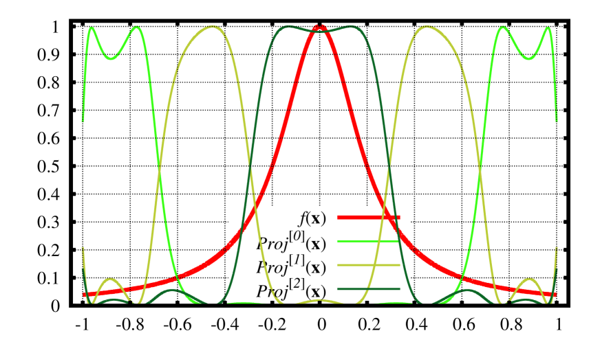
  Figure 3: Runge function (160) data (159) clustered to $D=3$. Corresponds to (152) data. The projections (22) to $\psi_{G}^{[m]}(\mathbf{x})$, $m=0\dots D-1$ are presented.

• The three function $\psi_{G}^{[m]}(\mathbf{x})$, corresponding to (152) nodes, are presented in Fig. 3. The $\mathrm{Proj}^{[i]}(\mathbf{x})$ (this is squared and normalized $\psi_{G}^{[m]}(\mathbf{x})$ as (22)). One can clearly see that the states $\psi_{G}^{[m]}(\mathbf{x})$ are localized exactly near the $f^{[m]}$ nodes (152). This technique is a much more powerful one, than, say, support–vector machine linear separation. In the Radon–Nikodym approach the separation weights are the $\left[\psi_{G}^{[m]}(\mathbf{x})\right]^{2}$ that are obtained without an introduction of a norm with subsequent minimization the difference between the result and a prediction with respect to the norm. The separation by the functions $\psi_{G}^{[m]}(\mathbf{x})$ is optimal among all $D$– dimensional separations of $\left[\psi(\mathbf{x})\right]^{2}$ type. The cost is that the solution is now two–step[3]. On the first step the Lebesgue quadrature is built and the measure (26) is obtained. On the second step the Gaussian quadrature (28) is built on this measure; the result is then converted to $\mathbf{x}$ space (30). The $\left[\psi_{G}^{[m]}(\mathbf{x})\right]^{2}$ are the optimal separation weights.

B.2 Nominal Attributes Example

In ML applications the attributes (1) can be nominal. They may be of orderable (low, medium, high) or unorderable (apple, orange, tomato) type. A nominal attribute taking two values can be converted to $\{0,1\}$ binary attribute. Orderable attributes (low, medium, high) can be converted to $\{1,2,3\}$, or, say, $\{1,2,10\}$ this depends on the problem. For unorderable attributes the conversion is more difficult, however in some situations it is straightforward: a ‘‘country’’ attribute taking the value: ‘‘country name from a list of eight countries’’, can be converted to three binary attributes.

The $f$, predicted by a ML system, is called class label. It is often a binary attribute. This leads to the nodes (15a) of the Lebesgue quadrature to be grouped near two values of the class label. We have tested a number of datasets from UC Irvine Machine Learning Repository, Weka datasets, and other sources. For direct comparison with the existing software such as C5.0 or Weka 3: Machine Learning Software in Java a care should be taken of nominal attributes conversion and class label representation. We are going to discuss the details in a separate publication, here we present only qualitative aspects of Radon–Nikodym approach application to ML problem with the binary class label. Take breast-cancer-wisconsin database, the breast-cancer-wisconsin.data dataset[30] is of $699$ records, we removed 16 records with unknown (‘‘?’’) attributes and split the dataset as 500:183 for training:testing. Obtained files are

wc breast-cancer-wisconsin_S.names \
   breast-cancer-wisconsin_S.data \
   breast-cancer-wisconsin_S.test
  139   938  6234 breast-cancer-wisconsin_S.names
  500   500 14266 breast-cancer-wisconsin_S.data
  183   183  5182 breast-cancer-wisconsin_S.test
  822  1621 25682 total

The data has nominal class label 2: Benign, 4:Malignant. C5.0, when run on this dataset produces a very good classifier:

c5.0  -f mldata/breast-cancer-wisconsin_S
Evaluation on training data (500 cases):
           (a)   (b)    <-classified as
          ----  ----
           293    10    (a): class 2
             3   194    (b): class 4
Evaluation on test data (183 cases):
           (a)   (b)    <-classified as
          ----  ----
           139     2    (a): class 2
             4    38    (b): class 4

Now let us run the RN program to obtain the Lebesgue quadrature

java com/polytechnik/utils/RN --data_cols=11:1,9:10:-1:0 \
   --data_file_to_build_model_from=mldata/breast-cancer-wisconsin_S.data \
   --data_file_evaluation=mldata/breast-cancer-wisconsin_S.test

The number of the nodes is 10, it is equal to the number of input attributes $x_{k}$.

$$f^{[0]} =2.090917684500027 w^{[0]} =308.30166232236996$$ (153)

$$f^{[1]} =3.198032991602546 w^{[1]} =5.307371268658678$$

$$f^{[2]} =3.344418191526764 w^{[2]} =0.0189894231470068$$

$$f^{[3]} =3.5619620739712725 w^{[3]} =0.3341989402039986$$

$$f^{[4]} =3.6221628167395497 w^{[4]} =0.2549558854552573$$

$$f^{[5]} =3.7509806530824346 w^{[5]} =1.2339290581894928$$

$$f^{[6]} =3.7939096228600513 w^{[6]} =5.146789024450902$$

$$f^{[7]} =3.8081118648848045 w^{[7]} =0.16082536035874645$$

$$f^{[8]} =3.8799894340830727 w^{[8]} =50.25004460556501$$

$$f^{[9]} =3.9574710127612613 w^{[9]} =128.99123411160124$$

Then we calculate a joint distribution of realization/prediction for $f_{RN}$ and $f_{RNW}$. The continuous to nominal conversion for $f_{RN}$ and $f_{RNW}$ was performed by comparing predicted value with the average. Evaluation without clustering on training data (154) (500 cases), and on test data (155) (183 cases) is:

$$\mathrm{Distribution}(f_{RN}) :\begin{matrix}183&120\\ 0&197\end{matrix} \mathrm{Distribution}(f_{RNW}) :\begin{matrix}294&9\\ 13&184\end{matrix}$$ (154)

$$\mathrm{Distribution}(f_{RN}) :\begin{matrix}91&50\\ 0&42\end{matrix} \mathrm{Distribution}(f_{RNW}) :\begin{matrix}140&1\\ 0&42\end{matrix}$$ (155)

We see that $f_{RN}$ that equally treats the states with low and high prior probability often gives spurious misclassifications. In the same time the $f_{RNW}$ that uses the projections adjusted to prior probability gives a superior prediction.

When we cluster to $D=2$:

java com/polytechnik/utils/RN --data_cols=11:1,9:10:-1:0 \
   --data_file_to_build_model_from=mldata/breast-cancer-wisconsin_S.data \
   --data_file_evaluation=mldata/breast-cancer-wisconsin_S.test \
   --clusters_number=2

$$f^{[0]} =2.09463398432689 w^{[0]} =310.52326905818705$$ (156)

$$f^{[1]} =3.924320437715293 w^{[1]} =189.47673094181317$$

The evaluation with $D=2$ clustering on training data (157) (500 cases) and on test data (158) (183 cases) gives joint distribution of realization/prediction for $f_{RN}$ and $f_{RNW}$:

$$\mathrm{Distribution}(f_{RN}) :\begin{matrix}292&11\\ 7&190\end{matrix} \mathrm{Distribution}(f_{RNW}) :\begin{matrix}295&8\\ 13&184\end{matrix}$$ (157)

$$\mathrm{Distribution}(f_{RN}) :\begin{matrix}141&0\\ 0&42\end{matrix} \mathrm{Distribution}(f_{RNW}) :\begin{matrix}141&0\\ 1&41\end{matrix}$$ (158)

Now, after the states with low prior probabilities (17a) are removed, both $f_{RN}$ and $f_{RNW}$ exhibit a good classification. For $D=3$, however, we still get a type of (154) and (155) behavior of spurious misclassifications by $f_{RN}$ and no such behavior in $f_{RNW}$.

This makes us to conclude that the $f_{RNW}$ answer is the superior answer for predicting a probabilistic $f$. The posterior distribution (17b) is Radon–Nikodym alternative to Bayes.

Appendix C RN Program Application With A Different Definition Of The Probability

Besides a typical ML classification problem the RN Program can be used for a number of different tasks, e.g. it can be applied to an interpolation problem. The reason is simple: as an input Radon–Nikodym only needs (7) matrices $F_{jk}$ and $G_{jk}$, which are calculated from (1) sample, that is a file of $M$ rows and $n+2$ columns ($n$ for $x_{k}$ and two for $f$ and the weight $\omega$). In the Appendix B the probabilities (7) were obtained as an ensemble average, calculated from the data, this is typical for a ML classification problem.

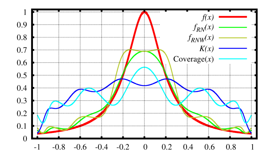
Figure 4: Runge function (160) interpolation result for $n=7$. The input data (1) was prepared (159) in a way the classification problem solver from Appendix B to reproduce interpolation results of the Appendix D of [13]. The $f_{RNW}(\mathbf{x})$ (18) (olive), Christoffel function (blue) (14), and the $\mathrm{Coverage}(\mathbf{x})$ (sky) (19) for the measure $\Braket{g}=\int_{-1}^{1}g(x)dx$ (161) are also calculated.

Input file can be constructed in a way that calculated averages represent a probability of different kind, such as time average probability. Consider function interpolation problem, the $\Braket{\cdot}$ now has a meaning of time–average $\Braket{g}=\int g(x)\omega(x)dx$, see Section II of [13]. A one–dimensional interpolation problem[7] can be reduced to (1) data by converting a two–columns sequence $x^{(l)}\to f^{(l)}$, $l=1\dots M$ to:

$$(1,x,x^{2},\dots,x^{n-1})^{(l)} \to f^{(l)} \omega^{(l)}$$ weight (159)

Because the result is invariant relatively any non–degenerated basis components linear transform any polynomials (e.g. $P_{m}(x)$, $T_{m}(x)$, etc.) can be used instead of the $x^{m}$ in (159). For example: to reproduce Runge function $d=1$ interpolation problem

$$f(x) =\frac{1}{1+25x^{2}}$$ (160)

$$d\mu =dx$$ (161)

$$x \in[-1:1]$$

for $n=7$, the result of the Appendix D of [13], take $x$ sequence with a small step about $dx=10^{-4}$, it will be about $M=1+2/dx$ total points $x\in[-1,-1+dx,-1+2dx,\dots,1-2dx,1-dx,1]$ and create a comma–separated file of $M$ rows and $n+2$ columns: $1,x,x^{2},\dots,x^{n-1},f(x),\omega$. First $n$ columns are the $\mathbf{x}$ from (159), then $f(x)$ from (160) follows, and the last column is the observation weight $\omega=dx$ for all points except the $dx/2$ for the edges. This file dataexamples/runge_function.csv is bundled with provided software. Run the program

java com/polytechnik/utils/RN --data_cols=9:0,6:7:8:1 \
      --data_file_to_build_model_from=dataexamples/runge_function.csv

The output file runge_function.csv.RN.csv has a few more columns, four of them are: the $f_{RN}$ from (13), the Christoffel function (14), the $f_{RNW}$ from (18), and the $\mathrm{Coverage}(\mathbf{x})$ (19). The result is presented in Fig. 4. With the data prepared as (159) the Christoffel–like function (14) is the regular Christoffel function for the measure (161). The $f_{RNW}(x)$ is also presented in Fig. 4. The $f_{RNW}(x)$, same as the $f_{RN}(x)$, is a weighted superposition (18) of (4) eigenvalues, but the weights are the posterior weights (17b), that are the product of prior weights by the $\Ket{\psi^{[i]}}$ projections: $w^{[i]}\mathrm{Proj}^{[i]}$. For Runge function in $n=7$ case only four prior weights (150) are non–zero, thus in Fig. 4 the $f_{RNW}(x)$ is a superposition of four eigenvalues. As we discussed above in Section II.1, the $f_{RN}(x)$ should be used for a deterministic functions, and the $f_{RNW}(x)$ is a solution to classification problem for a probabilistic $f$; it uses the posterior weights (17b). Same result can be also obtained using multi–index multiplications of Section V, take a single $x$ attribute and multiply it by itself 6 times. The quadrature will be identical.

java com/polytechnik/utils/RN --data_cols=9:0,1:7:8:1 \
      --max_multiindex=6 \
      --data_file_to_build_model_from=dataexamples/runge_function.csv

Radon–Nikodym interpolation [20] of an image ($d=2$ problem), can be performed in a similar way. Create a file of $M=d_{x}\times d_{y}$ rows and $n=n_{x}\times n_{y}+2$ columns. Each row corresponds to a single pixel. The last two columns are: pixel gray intensity and the weight (equals to 1). The first $n=n_{x}\times n_{y}$ columns are a function of pixel coordinate $(x_{l}\in 0\dots d_{x}-1,y_{l}\in 0\dots d_{y}-1)$ as $T_{j_{x}}(2\frac{x_{l}}{d_{x}-1}-1)T_{j_{y}}(2\frac{y_{l}}{d_{y}-1}-1)$, $j_{x}=0\dots n_{x}-1$, $j_{y}=0\dots n_{y}-1$. The $T_{m}(x)$ is Chebyshev polynomial $T_{0}=1;T_{1}=x;\dots$, they are chosen for numerical stability. In [20] the multi–index $\mathbf{j}=(j_{x},j_{y})$ has (53) and (54) constraints. After running the RN Program interpolated $f_{RN}$ and Christoffel function columns are added to output file, the $f_{RN}(x_{l},y_{l})$ provides required interpolation. While the Gaussian quadrature cannot be obtained for $d\geq 2$, the Christoffel function (10) can be easily calculated not only in $d\geq 2$ case, but also for an arbitrary $\mathbf{x}$ space with a measure $\Braket{\cdot}$.

The input file can be also constructed for $\mathbf{x}$ vector to represent a random variable. For example a distribution regression problem where a ‘‘bag’’ of observations is mapped to a single outcome $f$ can be approached[23] by using the moments of the distribution of a single ‘‘observations bag’’ as an input $\mathbf{x}$. For every ‘‘bag’’, calculate it’s distribution moments (one can use any choice of polynomials), then put these moments as $\mathbf{x}$ (now the $x_{k}$ components are the moments of the distribution of a bag’s instance), and use the $f$ as the outcome.

Similarly, temporal dependencies can be converted to (1) type of data. Assume $f$ has a $f(\mathbf{x}(t))$ form. Then each $x_{k}(t)$ can be converted to the moments $\Braket{Q_{s}(x_{k})}_{t}$, $s=0\dots n_{t}$, relatively some time–averaging $\Braket{\cdot}_{t}$ measure, such as in the Section II of [13]. Then the $n\times n_{t}$ input attributes $\Braket{Q_{s}(x_{k})}_{t}$, $k=0\dots n=1;s=0\dots n_{t}-1$, are ‘‘mixed’’ moments: time averaged $\Braket{\cdot}_{t}$ first and then ensemble averaged in (7). They can be used in (1) data input. Note, that ‘‘combined’’ averaging in (7) as $\Braket{\Braket{Q_{s}(x_{j}(t))}{Q_{s^{\prime}}(x_{k}(t))}_{t}}{$}producesdifferentresultthan``mixed^{\prime\prime}one:$⟨⟨Q_s(x_j(t))⟩_t| ⟨Q_s^′(x_k(t))⟩_t⟩$.Numericalexperimentsshowthat$⟨Q_s(x_k)⟩_t$attributestypicallyshowabetterresultthanusing$(x_k(t),x_k(t-δ),x_k(t-2δ),…)$asa``vectorish^{\prime\prime}$x_k$.Withtemporal(andspatial)attributesthedimensionof(\ref{mlproblem})inputcangrowveryfast.InsuchasituationSection\ref{BasisReduction}optimalclusteringisofcriticalimportance:thiswaywecanselectonlyafewcombinationsofinputattributes,thatoptimallyseparatethe$f$.\par\par ThestrengthoftheRadon--Nikodymapproachisthatitrequiresonlytwomatrices(\ref{matrixfxx})asaninput,andtheaverage$⟨⋅⟩$,usedtocalculatethe$F_jk$and$G_jk$,canbechosenwithadifferentdefinitionoftheprobability.Theinputfile(\texttt{\seqsplit{--data\_file\_to\_build\_model\_from=}}parameter)canbepreparedinaformtorepresentanyprobabilityspaceinanybasisofanydimension.Onerowcorrespondstoasinglerealization,allrowscorrespondtotheentiresample.Afterinputdatafileispreparedforthechosenprobabilityspace---thefeaturesintroducedinthispaper$f_RN(x),K(x),f_RNW(x),Coverage(x)$,alongwith$ψ_G^[m](x)$clusters(\ref{psiGclustersOpyatAZavor1e6})arecalculatedbythe\href http://www.ioffe.ru/LNEPS/malyshkin/code_polynomials_quadratures.zip.\par\par$

Appendix D A Numerical Solution to Quadratic Form Maximization Problem in Unitary Matrix Space

Consider a constrained optimization problem (128)

$${\mathcal{F}}=\sum\limits_{j,k,j^{\prime},k^{\prime}=0}^{n-1}{\mathcal{U}}_{jk}S_{jk;j^{\prime}k^{\prime}}{\mathcal{U}}^{*}_{j^{\prime}k^{\prime}} \xrightarrow[\mathcal{U}]{\quad}\max$$ (162)

$$\sum\limits_{k^{\prime}=0}^{n-1}{\mathcal{U}}_{jk^{\prime}}{\mathcal{U}}^{*}_{kk^{\prime}} =\delta_{jk}$$ (163)

This is a problem of optimization of scalar function (quadratic form with a Hermitian tensor $S_{jk;j^{\prime}k^{\prime}}$ from (130)) on the unitary group $U(n)$. It is equivalent to a problem of maximizing a quadratic form with a Hermitian matrix given multiple constraints (163) of quadratic form as well. The constraint may be of more general ‘‘partial unitarity $D\leq n$’’ form (197); a slight algorithm modification is then required, see Appendix G.1 below. A regular eigenvalue problem has a single quadratic form constraint, the problem in question has multiple. We have already approached a problem with an extra quadratic form constraint in the Appendix F of [9], the problem in question is of this type. Consider a ‘‘simplified constraint’’ (131)

$$\sum\limits_{j,k=0}^{n-1}{\mathcal{U}}_{jk}{\mathcal{U}}^{*}_{jk}=n$$ (164)

as a ‘‘partial’’ constraint for which optimization problem (162) can be readily converted to an eigenvalue problem to be directly solved. The idea is then to adjust obtained solution to satisfy full unitary constraints and calculate new values for Lagrange multipliers. Performing several iterations the process will converge to (162) optimization problem solution with the required constraints (163).

Consider Lagrange multipliers $\lambda_{jk}$ to optimize (162) with the constraints (163)

$$\sum\limits_{j,k,j^{\prime},k^{\prime}=0}^{n-1}{\mathcal{U}}_{jk}S_{jk;j^{\prime}k^{\prime}}{\mathcal{U}}^{*}_{j^{\prime}k^{\prime}}+\sum\limits_{j,k=0}^{n-1}\lambda_{jk}\left[\delta_{jk}-\sum\limits_{k^{\prime}=0}^{n-1}{\mathcal{U}}_{jk^{\prime}}{\mathcal{U}}^{*}_{kk^{\prime}}\right]\xrightarrow[\mathcal{U}]{\quad}\max$$ (165)

and variate it over all ${\mathcal{U}}_{jk}$ components. There are $2n^{2}$ real number coefficients defining ${\mathcal{U}}_{jk}=a_{jk}+ib_{jk}$, only $n^{2}$ of them are independent for a unitary matrix. One more coefficient is dropped as a common phase, so (162) optimization with the constraints (163) is equivalent to an unconstrained optimization problem over $n^{2}-1$ independent real parameters.

It is typically more convenient to variate (165) over ${\mathcal{U}}_{jk}$ and ${\mathcal{U}}^{*}_{jk}$ rather than over $a_{jk}$ and $b_{jk}$, then take care of the constraints by adjusting Lagrange multipliers $\lambda_{jk}$. The variations

$$0 =\sum\limits_{j^{\prime},k^{\prime}=0}^{n-1}{\mathcal{U}}_{j^{\prime}k^{\prime}}S_{j^{\prime}k^{\prime};pq}-\sum\limits_{j^{\prime}=0}^{n-1}\lambda_{j^{\prime}p}{\mathcal{U}}_{j^{\prime}q}$$ (166a)

$$0 =\sum\limits_{j^{\prime},k^{\prime}=0}^{n-1}S_{pq;j^{\prime}k^{\prime}}{\mathcal{U}}^{*}_{j^{\prime}k^{\prime}}-\sum\limits_{j^{\prime}=0}^{n-1}\lambda_{pj^{\prime}}{\mathcal{U}}^{*}_{j^{\prime}q}$$ (166b)

are consistent only when $\lambda_{jk}$ is a Hermitian matrix

$$\lambda_{jk} =\lambda^{*}_{kj}$$ (167)

From (166) also immediately follows: the functional (162) extremal value is equal to the spur of $\lambda_{jk}$:

$${\mathcal{F}}^{(extr)} =\sum\limits_{j=0}^{n-1}\lambda_{jj}$$ (168)

An algorithm finding extremal (162) is a generalization of the one from the Appendix F of [9] to multiple constraints:

1. Take initial $\lambda_{jk}$ and solve (165) optimization with partial constraint (164). Solution method – an eigenvalue problem of $n^{2}$ dimension in a vector space formed by writing all ${\mathcal{U}}_{jk}$ matrix elements in a vector, row by row. The result is: ${\mathcal{F}}$ and ${\mathcal{U}}_{jk}$ matrix reconstructed back from the eigenvector corresponding to maximal eigenvalue, row by row.

2. Obtained from this solution matrix ${\mathcal{U}}_{jk}$ may not be unitary as the constraint (164) is a subset of the full one (163). Expand ${\mathcal{U}}_{jk}$ in SVD

   $${\mathcal{U}}_{jk} =\sum\limits_{j^{\prime},k^{\prime}=0}^{n-1}U_{jj^{\prime}}\Sigma_{j^{\prime}k^{\prime}}V^{\dagger}_{k^{\prime}k}$$ (169)

   $$\widetilde{{\mathcal{U}}}_{jk} =\sum\limits_{j^{\prime}=0}^{n-1}U_{jj^{\prime}}V^{\dagger}_{j^{\prime}k}$$ (170)

   and adjust all SVD numbers to $1$: $\Sigma_{jk}=\delta_{jk}$, obtained $\widetilde{{\mathcal{U}}}_{jk}$ is a unitary matrix, it is the next iteration of the solution. This matrix (170) satisfies exact constraint (163), but the value of ${\mathcal{F}}$ is now increased. The $\widetilde{{\mathcal{U}}}_{jk}$ becomes a new ${\mathcal{U}}_{jk}$ at this iteration.

3. Put this new ${\mathcal{U}}_{jk}$ to (166a), then multiply it by ${\mathcal{U}}^{*}_{jq}$ and sum over $q=0\dots n-1$. As the ${\mathcal{U}}_{jk}$ is unitary $\lambda_{jk}=\sum_{p,q=0}^{n-1}\lambda_{jp}{\mathcal{U}}_{pq}{\mathcal{U}}^{*}_{kq}$ obtain new values for Lagrange multipliers $\widetilde{\lambda}_{jk}$ and take it’s Hermitian part:

   $$\widetilde{\lambda}_{jk} =\sum\limits_{j^{\prime},k^{\prime},q=0}^{n-1}{\mathcal{U}}_{j^{\prime}k^{\prime}}S_{j^{\prime}k^{\prime};kq}{\mathcal{U}}^{*}_{jq}$$ (171)

   $$\lambda_{jk} =\frac{1}{2}\left[\widetilde{\lambda}_{jk}+\widetilde{\lambda}^{*}_{kj}\right]$$ (172)

   This $\lambda_{jk}$ is the next iteration of Lagrange multipliers. As iterations proceed – the $\widetilde{\lambda}_{jk}$ should converge to a Hermitian matrix by itself, without (172) required.

4. Put this new $\lambda_{jk}$ to (165) and repeat iterational process until converged. On the first iteration take initial values for Lagrange multipliers as $\lambda_{jk}=0$.

Appendix E Non–Unitary Dynamics

In the previous section an approach to numerical solution of optimization problem (162) with unitary constraint (163) has been developed. Whereas for quantum systems time evolution operator ${\mathcal{U}}_{jk}$ can be only unitary, in data analysis it can possibly be of a non–unitary form. The difference arises because in data analysis wavefunction is directly ‘‘observable’’ (within a phase) with the goal to construct a ‘‘time evolution operator’’ (120).

The first non–unitary matrix of this type to consider is the (164), having a single constraint: the sum of squared elements is equal to $n$. With this matrix the problem can be easily solved. It does not preserve the normalizing, but gives more weight to correctly matched predictions. Regardless interpretation difficulties the dynamics with a matrix constrained the sum of squared elements being equal $n$ is the first one to try for the reasons of computational simplicity (no iterational process required) and mathematical interpretation simplicity (eigenvalue problem equivalence).

Another matrix of interest is a subspace-projection matrix. This type of constraint typically makes Lagrange multipliers $\lambda_{jk}$ calculation problematic, however some results can be obtained analytically, what makes a subspace-projection matrix the first one to try for an analytic study.

In the considered above approach to dynamics the $\mathbf{x}^{(l)}$ and $\mathbf{x}^{(l+1)}$ were belong to the same phase space. It is of great interest to consider a situation where $\Ket{\psi_{\mathbf{x}^{(l)}}}$ and $\Ket{\psi_{\mathbf{x}^{(l+1)}}}$ belong to different vector spaces, e.g. to use $\Ket{\psi_{\mathbf{f}^{(l)}}}$ instead of $\Ket{\psi_{\mathbf{x}^{(l+1)}}}$. In this case in (120) operator ${\mathcal{U}}$ is transforming $\Ket{\psi_{\mathbf{x}}}$ to a different vector space $\Ket{\psi_{\mathbf{f}}}$; this is not a true ‘‘dynamics’’ ($l$ is the same), but such a transform can be applied to a traditional ML classification problem.

While a study of a general non–unitary $\mathbf{x}\to\mathbf{f}$ homomorphism producing the most general form of non–unitary dynamics is out of scope of this work (see Appendix I below for our first attempt), let us consider a simple composition of a unitary transformation ${\mathcal{U}}$: $\mathbf{x}\to\mathbf{x}$ followed by projection of $\mathbf{x}$ on $\mathbf{f}$, a ‘‘projective’’ form of non–unitary dynamics. Let us apply it to a vector–to–vector classification problem of Section VI.2. Assume we have a problem with vector–valued class label (62)

$$\mathbf{x}^{(l)} \to\mathbf{f}^{(l)} \text{weight $\omega^{(l)}$};l=1\dots M$$ (173)

The choice of knowledge representation is the most important feature of a ML approach. For example it can be a linear regression (84), a ratio of two quadratic forms (66) or (68), neural network weights, etc. An important result of this appendix is to consider not $\mathbf{x}\to\mathbf{f}$ mapping, but instead to construct localized wavefunctions (24) in $\mathbf{x}$- and $\mathbf{f}$- space: $\psi_{\mathbf{y}}(\mathbf{x})$ and $\psi_{\mathbf{g}}(\mathbf{f})$ to study $\psi_{\mathbf{y}}(\mathbf{x})$ mapping with a unitary operator ${\mathcal{U}}$ in $\mathbf{x}$-space following by a projection of the transform $\Ket{{\mathcal{U}}|\psi_{\mathbf{y}}}$ on $\mathbf{f}$-space outcome $\psi_{\mathbf{g}}(\mathbf{f})$:

$$\mathrm{Prob}(\mathbf{g}|\mathbf{y})=\left|\Braket{\psi_{\mathbf{g}}}{{\mathcal{U}}}{\psi_{\mathbf{y}}}\right|^{2} 1\geq\varpi(\mathbf{g})\geq\mathrm{Prob}(\mathbf{g}|\mathbf{y})$$ (174)

$${\mathcal{F}}=\sum\limits_{l=1}^{M}\omega^{(l)}\left|\Braket{\psi_{\mathbf{f}^{(l)}}}{{\mathcal{U}}}{\psi_{\mathbf{x}^{(l)}}}\right|^{2}=\sum\limits_{l=1}^{M}\omega^{(l)}\mathrm{Prob}(\mathbf{f}^{(l)}|\mathbf{x}^{(l)})$$ (175)

$$\mathrm{Error}=\Braket{1}-{\mathcal{F}}$$ (176)

Conditional probability (174) is bounded by the value $\varpi(\mathbf{g})$ of full basis expansion (91), a situation without predictor available, this is the problem we considered in Section VI.2 above. Because $\mathbf{x}$- and $\mathbf{f}$- space are different – a projection of a wavefunction from one to another gives $1\geq\varpi(\mathbf{g})\geq\left|\Braket{\psi_{\mathbf{g}}}{{\mathcal{U}}}{\psi_{\mathbf{y}}}\right|^{2}$ in (174). This non–unitarity, however, does not create any practical difficulties as we separated a ‘‘unitary dynamics’’ in $\mathbf{x}$-space and a ‘‘non–unitary projection’’ to $\mathbf{f}$-space. The (176) error estimator has the meaning of misclassified observations number, it is bounded by considered above simple projective estimator (89); it is zero if $\mathbf{f}$ is a subspace of $\mathbf{x}$ (in (182) below consider $\Psi$ as a direct sum of $\Phi$ and the space orthogonal to $\Phi$, then in (184) numerator cancels denominator).

Given the expressions (24) for $\psi_{\mathbf{y}}(\mathbf{x})$ and for $\psi_{\mathbf{g}}(\mathbf{f})$:

$$\psi_{\mathbf{g}}(\mathbf{f}) =\frac{\sum\limits_{j,k=0}^{m-1}g_{j}G^{\mathbf{f};\,-1}_{jk}f_{k}}{\sqrt{\sum\limits_{j,k=0}^{m-1}g_{j}G^{\mathbf{f};\,-1}_{jk}g_{k}}}$$ (177)

here $G^{\mathbf{f};\,-1}_{jk}$ is an inverse of $G^{\mathbf{f}}_{jk}$ from (79), we can write conditional probability (174) as:

$$\mathrm{Prob}(\mathbf{g}|\mathbf{y}) =\frac{\left|\sum\limits_{j,k,p=0}^{n-1}\sum\limits_{j^{\prime},k^{\prime}=0}^{m-1}y_{j}G^{\mathbf{x};\,-1}_{jk}u_{kp}G^{\mathbf{x}\mathbf{f}}_{pj^{\prime}}G^{\mathbf{f};\,-1}_{j^{\prime}k^{\prime}}g_{k^{\prime}}\right|^{2}}{\sum\limits_{j,k=0}^{n-1}y_{j}G^{\mathbf{x};\,-1}_{jk}y_{k}\sum\limits_{j^{\prime},k^{\prime}=0}^{m-1}g_{j^{\prime}}G^{\mathbf{f};\,-1}_{j^{\prime}k^{\prime}}g_{k^{\prime}}}$$ (178)

$$\Ket{{\mathcal{U}}|x_{k}} =\sum\limits_{p=0}^{n-1}u_{kp}x_{p}$$ (179)

The expression is very similar to (99), the difference is that instead of $G^{\mathbf{x}\mathbf{f}}_{kj^{\prime}}$ we now have $\mathbf{x}$ transformed by a unitary operator ${\mathcal{U}}$ as $\sum_{p=0}^{n-1}u_{kp}G^{\mathbf{x}\mathbf{f}}_{pj^{\prime}}$. This is the key difference: instead of ‘‘direct projection’’ we now have a unitary transformation and then a projection. In

$${\mathcal{F}} =\sum\limits_{l=1}^{M}\omega^{(l)}\mathrm{Prob}(\mathbf{f}^{(l)}|\mathbf{x}^{(l)})=\sum\limits_{j,k,p,q=0}^{n-1}u_{jk}S_{jk;pq}u^{*}_{pq}$$ (180)

a Hermitian tensor $S_{jk;pq}$ is readily obtained from (178) and (180) with simple algebra. Thus we reduced $\mathbf{x}\to\mathbf{f}$ classification problem to a dynamic problem of finding a unitary matrix maximizing (180), i.e. the problem considered in Section D! This is the most general solution to a vector class label classification problem, it finds a unitary transformation ${\mathcal{U}}$ (179), producing the maximal coverage in (180).

Note, that unitary operator ${\mathcal{U}}$ coefficients $u_{kp}$ are defined in (179) in a general, non–orthogonal basis $x_{k}$, a one with real symmetric Gram matrix $G_{jk}^{\mathbf{x}}=\Braket{x_{j}x_{k}}$. This makes unitarity constraint more verbose:

$$G_{pq}^{\mathbf{x}} =\sum\limits_{j,k=0}^{n-1}u_{pj}G_{jk}^{\mathbf{x}}u^{*}_{qk}$$ (181)

It is convenient to select orthogonal bases $\Psi^{[i]}(\mathbf{x})$, $i=0\dots n-1$ and $\Phi^{[j]}(\mathbf{f})$, $j=0\dots m-1$ for input data, we already did this in Eq. (121) above:

$$\Psi^{[i]}(\mathbf{x}) =\sum\limits_{k=0}^{n-1}B^{\mathbf{x}}_{ik}x_{k} i=0\dots n-1$$ (182)

$$s_{i}^{(l)} =\Braket{\psi_{\mathbf{x}^{(l)}}}{\Psi^{[i]}}=\frac{\Psi^{[i]}(\mathbf{x}^{(l)})}{\sqrt{\sum\limits_{j=0}^{n-1}\left|\Psi^{[j]}(\mathbf{x}^{(l)})\right|^{2}}} 1=\sum\limits_{i=0}^{n-1}\left|s_{i}^{(l)}\right|^{2}$$

$$\delta_{pq} =\Braket{\Psi^{[p]}}{\Psi^{[q]}}=\sum\limits_{j,k=0}^{n-1}B^{\mathbf{x}}_{pj}G_{jk}^{\mathbf{x}}B^{\mathbf{x}}_{qk} p,q=0\dots n-1$$

$$\Phi^{[i]}(\mathbf{f}) =\sum\limits_{k=0}^{m-1}B^{\mathbf{f}}_{ik}f_{k} i=0\dots m-1$$ (183)

$$d_{i}^{(l)} =\Braket{\psi_{\mathbf{f}^{(l)}}}{\Phi^{[i]}}=\frac{\Phi^{[i]}(\mathbf{f}^{(l)})}{\sqrt{\sum\limits_{j=0}^{m-1}\left|\Phi^{[j]}(\mathbf{f}^{(l)})\right|^{2}}} 1=\sum\limits_{i=0}^{m-1}\left|d_{i}^{(l)}\right|^{2}$$

$$\delta_{pq} =\Braket{\Phi^{[p]}}{\Phi^{[q]}}=\sum\limits_{j,k=0}^{m-1}B^{\mathbf{f}}_{pj}G_{jk}^{\mathbf{f}}B^{\mathbf{f}}_{qk} p,q=0\dots m-1$$

As the solution is gauge–invariant relatively (65) we can use any basis. An orthogonal basis choice is also beneficial for computational complexity: it takes $O(n)$ instead of $O(n^{2})$ to calculate a quadratic form $\sum_{j,k=0}^{n-1}y_{j}G^{\mathbf{x};\,-1}_{jk}y_{k}$ in a basis in which $G_{jk}^{\mathbf{x}}$ is diagonal. The $\mathrm{Prob}(\Phi|\Psi)$ also takes a much simpler form:

$$\mathrm{Prob}(\mathbf{f}|\mathbf{x}) =\mathrm{Prob}(\Phi|\Psi)=\frac{\left|\sum\limits_{j,k=0}^{n-1}\sum\limits_{i=0}^{m-1}\Psi^{[j]}{\mathcal{U}}_{jk}G^{\Psi\Phi}_{ki}\Phi^{[i]}\right|^{2}}{\sum\limits_{j=0}^{n-1}\left|\Psi^{[j]}\right|^{2}\sum\limits_{i=0}^{m-1}\left|\Phi^{[i]}\right|^{2}}$$ (184)

$$G^{\Psi\Phi}_{ki} =\Braket{\Psi^{[k]}\Phi^{[i]}}=\sum\limits_{j=0}^{n-1}\sum\limits_{j^{\prime}=0}^{m-1}B^{\mathbf{x}}_{kj}G^{\mathbf{x}\mathbf{f}}_{jj^{\prime}}B^{\mathbf{f}}_{ij^{\prime}}$$ (185)

$$S_{jk;pq} =\sum\limits_{l=1}^{M}\omega^{(l)}\sum\limits_{r,t=0}^{m-1}s_{j}^{(l)}G^{\Psi\Phi}_{kr}d_{r}^{(l)}s_{p}^{(l)}G^{\Psi\Phi}_{qt}d_{t}^{(l)}$$ (186)

The (186) corresponds to (127) when put formally $s_{k}^{(l+1)}=\sum_{j=0}^{m-1}G^{\Psi\Phi}_{kj}d_{j}^{(l)}$ and swap tensor indexes (inverse time): $\overset{\looparrowleft}{S}_{jk;pq}=S_{kj;qp}$. A unitary operator ${\mathcal{U}}$ now has a matrix ${\mathcal{U}}_{jk}$ with regular unitarity constraint (163). As the result is basis–independent it is practically convenient to use input data $x_{k}^{(l)}$ and $f_{j}^{(l)}$ to calculate the matrices (79) and (80), then build from them the bases (182) and (183), with possible regularization of the Appendix A, then finally use $\Psi^{[k]}(\mathbf{x}^{(l)})$ and $\Phi^{[j]}(\mathbf{f}^{(l)})$ as they were input data sample. In new bases the problem with Hermitian tensor (186) can be directly approached by (162) optimization with unitary constraint (163). Obtained solution is independent on bases $\Psi^{[k]}$ and $\Phi^{[j]}$ specific choice (gauge–invariant). If contributing subspace is known explicitly the solution of dimension $n$ can be reduced to $m$ using clustering approach (195) of Appendix G below; there is also a general $D$-clusters solution corresponding to a more general ‘‘partial unitarity $D\leq n$’’ form of constraint (197).

What is the main application of the approach of this appendix? Most often – it is a ‘‘replacement’’ of a regression in a problem of recovering some hidden $\mathbf{x}\to\mathbf{f}$ relation. Both theories take (173) data as input and have zero error if $\mathbf{f}$ is a subspace of $\mathbf{x}$. The differences can be summarized in the table:

	Regression	‘‘Dynamic’’ theory
The Result	Function value $\mathbf{f}(\mathbf{x})$ (84); diverges at $\mathbf{x}\to\infty$	Conditional probability $\mathrm{Prob}(\mathbf{f}|\mathbf{x})$ (184); does not diverge at $\mathbf{x}\to\infty$
Optimization	$L^{2}$ norm (2) in $\mathbf{f}$-space	The number of correctly classified observations (175)
Mathematical problem	Linear system solution	Conditional optimization (162) with unitary constraint (163)
Outliers and fat tail sensitivity	Very sensitive; a single ‘‘several orders off’’ outlier completely invalidates the solution	Not sensitive; a single outlier may invalidate only a single observation point
Symmetry $\psi\to-\psi$	Broken: observable is linear on $\mathbf{x}$; $\psi$ is also linear on $\mathbf{x}$.	Preserved: $\psi$ is linear on $\mathbf{x}$, but the probability (174) behaves as $\psi^{2}$, invariant with: $\psi_{\mathbf{x}}\to-\psi_{\mathbf{x}}$; $\psi_{\mathbf{f}}\to-\psi_{\mathbf{f}}$
Physical world relation	A model	Most of dynamic equations in nature are equivalent to a sequence of unitary transformations (Newton, Maxwell, Schrödinger equations)

Appendix F A Projective Non–Unitary Dynamics

Considered in Section E projective dynamics consists in a unitary transformation of $\mathbf{x}$ following by a projection of the transform on $\mathbf{f}$. The problem can be further generalized. Consider input data (173) as vector spaces $\mathbf{x}$ and $\mathbf{f}$ (it is convenient to convert them to $\Psi$ and $\Phi$ of Eqs. (182) and (183)). The $\Psi$ and $\Phi$ are regular vector spaces of the dimensions $n$ and $m$ with a scalar product determined by positively defined (otherwise apply Appendix A regularization) matrices (79) and (80) calculated from the data sample (173). In addition we have a ‘‘cross–product’’ $\Braket{\Psi}{\Phi}$ (185) determined by the matrix $G^{\mathbf{x}\mathbf{f}}_{jk^{\prime}}$ (81) calculated from the same data sample. These bases may not be full with respect to each other:

$$1 \geq\sum\limits_{j=0}^{m-1}\Braket{\Psi^{[i]}\Phi^{[j]}}^{2} i=0\dots n-1$$ (187a)

$$1 \geq\sum\limits_{j=0}^{n-1}\Braket{\Psi^{[j]}\Phi^{[i]}}^{2} i=0\dots m-1$$ (187b)

In Section VI.1 we considered an approach of various $\Psi\leftrightarrow\Phi$ projections. In Appendix E we considered a composition of a unitary transformation ${\mathcal{U}}^{\Psi}$ $\Psi\to\Psi$ following by a projection of the transform on $\Phi$. In this appendix we consider the most general case, a composition of:

1. A $\Psi\to\Psi$ unitary transformation ${\mathcal{U}}^{\Psi}$, the transform is $\Ket{{\mathcal{U}}^{\Psi}|\Psi}$.

2. A $\Phi\to\Phi$ unitary transformation ${\mathcal{U}}^{\Phi}$, the transform is $\Ket{{\mathcal{U}}^{\Phi}|\Phi}$.

3. Projection of these two transforms on each other: $\Braket{\Phi}{{\mathcal{U}}^{\Phi}}{{\mathcal{U}}^{\Psi}|\Psi}$ using (185) ‘‘scalar product’’.

The number of ‘‘covered’’ observations is then:

$$\mathrm{Prob}(\mathbf{f}|\mathbf{x}) =\mathrm{Prob}(\Phi|\Psi)=\left|\Braket{\Phi}{{\mathcal{U}}^{\Phi}}{{\mathcal{U}}^{\Psi}|\Psi}\right|^{2}$$ (188)

$${\mathcal{F}} =\sum\limits_{l=1}^{M}\omega^{(l)}\left|\Braket{\Phi_{\mathbf{f}^{(l)}}}{{\mathcal{U}}^{\Phi}}{{\mathcal{U}}^{\Psi}|\Psi_{\mathbf{x}^{(l)}}}\right|^{2}=\sum\limits_{l=1}^{M}\omega^{(l)}\mathrm{Prob}(\mathbf{f}^{(l)}|\mathbf{x}^{(l)})$$ (189)

These expressions are different from (174) and (175) in a second unitary transformation $\|{\mathcal{U}}^{\Phi}\|$. The problem is then: Maximize (189) over ${\mathcal{U}}^{\Psi}_{jk}$ and ${\mathcal{U}}^{\Phi}_{jk}$ given two unitary constraints:

$$\delta_{jk} =\sum\limits_{i=0}^{n-1}{\mathcal{U}}^{\Psi}_{ji}{\mathcal{U}}^{\Psi\,*}_{ki} j,k=0\dots n-1$$ (190a)

$$\delta_{jk} =\sum\limits_{i=0}^{m-1}{\mathcal{U}}^{\Phi}_{ji}{\mathcal{U}}^{\Phi\,*}_{ki} j,k=0\dots m-1$$ (190b)

The optimization (189) with the constraints (190) can be approached by Appendix D type of algorithm, however, as (189) is a quadratic form over matrix elements products ${\mathcal{U}}^{\Psi}_{jk}{\mathcal{U}}^{\Phi}_{qp}$ (a ‘‘two–particle’’ system wavefunction basis is a product of individual particles wavefunction), this makes the problem of dimensions product, thus makes it impractical. We expect that a heuristic algorithm, such as alternately optimize (189) over ${\mathcal{U}}^{\Psi}_{jk}$ and ${\mathcal{U}}^{\Phi}_{qp}$, can be a better fit. For isomorphic $\mathbf{f}$-space and $\mathbf{x}$-space ($n=m$ and all coefficients in (187) are equal to $1$) the dynamics is unitary and the problem itself becomes degenerated: It then depends on a single operator $\|{\mathcal{U}}\|=\|{\mathcal{U}}^{\Psi}|{\mathcal{U}}^{\Phi}\|$ what is equivalent to the problem already considered in Section VI.5. This makes us to conclude that considered in Section E composition: a unitary transformation of $\Psi$ following by a projection of the transform on $\Phi$ is the most practical approach to traditional ML classification problem $\mathbf{x}\to\mathbf{f}$.

Appendix G On Clustering of a Dynamic System Phase Space

In Appendix E a ‘‘projective’’ solution to dynamic system identification problem has been developed. The solution has the form of a unitary operator $\|{\mathcal{U}}\|$ in $\mathbf{x}$-space. Conditional probability given possible input/output is determined by (174) projection of $\mathbf{x}$ vector transform to a vector in $\mathbf{f}$-space. The dimension of $\mathbf{x}$-space and $\mathbf{f}$-space can be quite different. The $n$ is typically of hundreds, often thousands, for a system with internal state (memory), see Appendix H below, it may reach millions. The $m$ is the dimension of $\mathbf{f}$, the number of values of interest, it is always below a few dozen. From this relation naturally arises the problem of clustering: to construct a low dimension $D<n$ subspace of phase space $\mathbf{x}$ that captures most of the information about $\mathbf{f}$. For a problem with vector class label only the case $D=m$ is easy.

Consider some orthogonal basis $\Ket{\psi^{[i]}}$ in $\mathbf{x}$-space and expand $\mathbf{x}^{(l)}$-localized states $\psi_{\mathbf{x}^{(l)}}(\mathbf{x})$ in this basis:

$$\Ket{\psi_{\mathbf{x}^{(l)}}} =\sum\limits_{i=0}^{n-1}\Braket{\psi_{\mathbf{x}^{(l)}}}{\psi^{[i]}}\Ket{\psi^{[i]}}$$ (191)

then substitute to (175), obtain the number of covered observations:

$${\mathcal{F}} =\sum\limits_{l=1}^{M}\omega^{(l)}\left|\Braket{\psi_{\mathbf{f}^{(l)}}}{{\mathcal{U}}}{\psi_{\mathbf{x}^{(l)}}}\right|^{2}$$

$$=\sum\limits_{l=1}^{M}\omega^{(l)}\sum\limits_{i,j=0}^{n-1}\Braket{\psi^{[i]}}{\psi_{\mathbf{x}^{(l)}}}\Braket{\psi^{[i]}}{{\mathcal{U}}^{\dagger}}{\psi_{\mathbf{f}^{(l)}}}\Braket{\psi_{\mathbf{f}^{(l)}}}{{\mathcal{U}}}{\psi^{[j]}}\Braket{\psi_{\mathbf{x}^{(l)}}}{\psi^{[j]}}$$ (192)

Were we operate in terms of simple ‘‘projective paradigm’’ of Section VI.2 this would correspond to (94) error with (96) spectral expansion. Now, however, the problem is that sought basis $\Ket{\psi^{[i]}}$ enters (192) coverage four times, thus a direct eigenvalues expansion is no longer possible. As the conditional probablities are bounded (174) by direct projection to the entire $\mathbf{x}$-space by probabilities (91), obtain ${\mathcal{F}}$ upper bound:

$${\mathcal{F}}^{DP} =\sum\limits_{l=1}^{M}\omega^{(l)}\varpi(\mathbf{f}^{(l)}) {\mathcal{F}}\leq{\mathcal{F}}^{DP}$$ (193)

The spectral expansion (96) has at most $m$ eigenvectors (95) contributing to coverage expansion with $\Ket{\psi_{\mathbf{f}^{(l)}}}$, for (192) this means that only these $\Ket{\phi}$ contribute to coverage:

$$\Ket{\psi^{[i]}} \in\Ket{{\mathcal{U}}|\phi}$$ (194)

where $\Ket{\psi^{[i]}}$ belongs to (95) eigenvectors subset having non–zero eigenvalue, there are at most $m$ out of total $n$. From this follows that only vector space $\Ket{\phi^{[i]}}$ contribute:

$$\Ket{\phi^{[i]}} =\Ket{{\mathcal{U}}^{\dagger}|\psi^{[i]}}$$ (195)

where $i$ takes $m$ out of $n$ values such that $\lambda^{[i]}>0$ in (95). The $\Ket{\phi^{[i]}}$ is the only $\mathbf{x}$-subspace contributing to total coverage (192).

Appendix D solution to maximization (192) (which is a quality criterion) finds unitary matrix $\|{\mathcal{U}}\|$ in $\mathbf{x}$-space of the dimension $n$. However, as quality criterion operates in $\mathbf{f}$-space of the dimension $m$, the transform (195) allows to build $\mathbf{x}$-subspace of the dimension $D=m$ as the only vector subspace contributing to quality criterion.

For a system with known contributing subspace numerical optimization algorithm of Appendix D can be optimized by converting the basis to contributing subspace and simplifying the constraints to act in contributing subspace only, i.e. considering a subset of a full set of unitarity constraints. The conversion back from contributing subspace to $\mathbf{x}$-space then requires some algebra as the condition for unitary operators; ${\mathcal{U}}^{-1}={\mathcal{U}}^{\dagger}$ may no longer hold true in full $\mathbf{x}$-space.

In practice the problem of finding the contributing subspace (95) is typically ‘‘an extra step’’, thus it is sometimes more convenient to solve the problem directly to avoid a non-unitary transformation between contributing subspace and $\mathbf{x}$-space. Whereas constructing a $\mathbf{f}$-predictor of given input dimension $D\leq n$ creates the same problem as with (192) (an expression with the fourth power of sought basis), the problem of finding $\mathbf{x}$ subspace of the dimension $D\leq n$ providing maximal coverage on $\mathbf{f}$, can be directly reduced to a variant of Appendix D optimization problem.

Consider coverage maximization problem with constraints:

$${\mathcal{F}} =\sum\limits_{l=1}^{M}\omega^{(l)}\sum\limits_{j=0}^{D-1}\Braket{\psi_{\mathbf{f}^{(l)}}}{\phi^{[j]}}^{2}\xrightarrow[\phi]{\quad}\max$$ (196)

$$\delta_{jk} =\Braket{\phi^{[j]}}{\phi^{[k]}} j,k=0\dots D-1$$ (197)

the goal is to find an orthogonal basis $\phi^{[j]}(\mathbf{x})$ of dimension $D\leq n$, $j=0\dots D-1$, providing maximal (196) coverage; the solution is non-unique, it is (95) eigenvectors, corresponding to $D$ largest eigenvalues within an arbitrary unitary transformation of them. The problem (91) of above corresponds to $D=n$ case; (193) is the upper bound of (196). Here $\psi_{\mathbf{g}}(\mathbf{f})$ is $\mathbf{f}=\mathbf{g}$ localized state (177) in $\mathbf{f}$-space, and $\phi^{[j]}(\mathbf{x})$ is $\mathbf{x}$-space linear function:

$$\phi^{[j]}(\mathbf{x}) =\sum\limits_{k=0}^{n-1}u_{jk}x_{k} j=0\dots D-1$$ (198)

Substituting (198) to (196) obtain optimization problem with some $S_{jk;j^{\prime}k^{\prime}}$:

$${\mathcal{F}}=\sum\limits_{j,j^{\prime}=0}^{D-1}\sum\limits_{k,k^{\prime}=0}^{n-1}u_{jk}S_{jk;j^{\prime}k^{\prime}}u^{*}_{j^{\prime}k^{\prime}} \xrightarrow[u]{\quad}\max$$ (199)

$$\sum\limits_{k,k^{\prime}=0}^{n-1}u_{jk}G^{\mathbf{x}}_{kk^{\prime}}u^{*}_{ik^{\prime}} =\delta_{ji} j,i=0\dots D-1$$ (200)

The problem: to find $u_{jk}$ matrix of the dimensions $j=0\dots D-1,k=0\dots n-1$, providing maximal (199) subject to constraint (200). Obtained $u_{jk}$ matrix defines $\phi^{[j]}(\mathbf{x})$ basis (198) of the dimension $D\leq n$ providing maximal coverage in (196). This basis is then typically used to construct in it a unitary operator ${\mathcal{U}}$ providing maximal coverage in (175). Thus we need to solve two optimization problems: first (196) to construct a basis of lower dimension, second (175) to build a unitary operator in this basis. If $D=m$ and $\mathbf{f}$ is a subspace of $\mathbf{x}$ then the sought basis is this subspace and coverage is maximal ${\mathcal{F}}=\Braket{1}$. Otherwise we modify Appendix D algorithm to $D\leq n$ case, specifically:

G.1 A Numerical Solution to Quadratic Form Maximization Problem With Partial Unitarity Constraint

Without loss of generality let $G^{\mathbf{x}}_{kk^{\prime}}=\delta_{kk^{\prime}}$, i.e. the problem is considered in bases (182) and (183). Optimization problem is then:

$${\mathcal{F}}=\sum\limits_{j,j^{\prime}=0}^{D-1}\sum\limits_{k,k^{\prime}=0}^{n-1}u_{jk}S_{jk;j^{\prime}k^{\prime}}u^{*}_{j^{\prime}k^{\prime}} \xrightarrow[u]{\quad}\max$$ (201)

$$\sum\limits_{k=0}^{n-1}u_{jk}u^{*}_{ik} =\delta_{ji} j,i=0\dots D-1$$ (202)

Consider Lagrange multipliers $\lambda_{jj^{\prime}}$, a matrix of $D\times D$ dimension, to optimize (201) with the constraints (202)

$$\sum\limits_{j,j^{\prime}=0}^{D-1}\sum\limits_{k,k^{\prime}=0}^{n-1}u_{jk}S_{jk;j^{\prime}k^{\prime}}u^{*}_{j^{\prime}k^{\prime}}+\sum\limits_{j,j^{\prime}=0}^{D-1}\lambda_{jj^{\prime}}\left[\delta_{jj^{\prime}}-\sum\limits_{k^{\prime}=0}^{n-1}u_{jk^{\prime}}u^{*}_{j^{\prime}k^{\prime}}\right]\xrightarrow[u]{\quad}\max$$ (203)

The variations are consistent only when $\lambda_{jj^{\prime}}$ is a Hermitian matrix. The ‘‘partial’’ constraint is the squared Frobenius norm condition:

$$\sum\limits_{j=0}^{D-1}\sum\limits_{k=0}^{n-1}u_{jk}u^{*}_{jk}=D$$ (204)

with which (201) optimization can be reduced to a generalized eigenvalue problem. Then repeat Appendix D iteration almost identically. Generalized eigenvalue problem of the dimension $Dn$ is solved with partial constraint (204) being wavefunction normalizing condition; obtained with partiall constrained solution $u_{jk}$ requires an adjustment to satisfy full constraint (202); it is performed using SVD expansion:

$$u_{jk} =\sum\limits_{j^{\prime}=0}^{D-1}\sum\limits_{k^{\prime}=0}^{n-1}U_{jj^{\prime}}\Sigma_{j^{\prime}k^{\prime}}V^{\dagger}_{k^{\prime}k}$$ (205)

followed by setting diagonal elements of the rectangular diagonal matrix $\Sigma_{jk}$ to $1$; new values for Lagrange multipliers $\lambda_{jj^{\prime}}$ are then calculated from adjusted $u_{jk}$ to perform a new iteration. With these changes to Appendix D algorithm the iterational process produces $u_{jk}$ matrix maximizing (201) subject to partial unitarity $D\leq n$ constraint (202).

Appendix H The Dynamics of a System with Internal State

The data (173) $\mathbf{x}^{(l)}\to\mathbf{f}^{(l)}$ is the form most frequently studied in ML, where observations corresponding to different $l$ are considered as independent observations. Same data studied in signal processing is typically considered as $l$–ordered (e.g. $l$ is time), where the problem of timeserie prediction corresponds to $\mathbf{f}^{(l)}=\mathbf{x}^{(l+1)}$. Such an embedding of timeserie data to (173) implicitly selects a time–scale. Real system have some internal state $\mathbf{z}$ (memory); the output now depends not only on the input signals $\mathbf{x}$, but also on the internal state $\mathbf{z}$:

$$\left(\mathbf{x}^{(l)},\mathbf{z}^{(l)}\right) \to\mathbf{f}^{(l)} \text{weight $\omega^{(l)}$};l=1\dots M$$ (206)

This produces a omnifarious dynamics, much richer compared to systems without internal state. An example of a system with memory is a finite-state machine. From practical point of view it is convenient to classify them as the systems with:

• Completely observable internal state.

• Partially observable internal state.

The same system (e.g. a vending machine) can be completely observable to a support team (have a full access to vending machine memory) and partially observable to a customer (can only see whether it is empty and not working). In this appendix we will be only considering the systems with completely observable internal state.

Consider a very simple finite-state machine: synchronous positive-edge-triggered D flip-flop (D trigger); it’s circuit has a positive feedback loop what creates a bistable system. CD4013 chip is a typical example of this device.

(207)

It operates as following: on every $0\to 1$ transition on $C$ (on the rising edge LH of the clock) input $D$ is recorded and becomes immediately available on $Q$, the $\overline{Q}$ is it’s inverse. Any changes on $D$ has no effect on the state unless there is a rising edge on $C$:

C D Q LH 0 0 LH 1 1 0 1 HL X unchanged (215)

This device can be used as a 1-bit memory register, pulses counter, frequency divider by 2 (connect $D$ with $\overline{Q}$ to inverse the state on every LH on $C$), etc.

Consider a simple problem of the dimensions $n=2$, $m=1$. Take edge–triggered D flip-flop, let $x_{0}=D$, $x_{1}=C$, and output $f=Q$. Also assume (to avoid timing considerations) that on every tick $l$ the $x_{1}^{(l)}$ takes the value slightly after $x_{0}^{(l)}$ was set. The output $Q$ at $l$ now depends not only on current input $\mathbf{x}^{(l)}$ but also on the previous state (and hence, previous inputs). Now assume that all the input $\mathbf{x}^{(l)}$ are completely random. For every new $l$–th input $\mathbf{x}^{(l)}$ coming (completely random) the system undergo transition:

$$f^{(l)} =\begin{cases}x_{0}^{(l)}&\text{if $x_{1}^{(l-1)}=0$ and $x_{1}^{(l)}=1$}\\ f^{(l-1)}&\text{otherwise}\end{cases}$$ (216)

It is clear that this D-trigger cannot be predicted by $n=2$, $m=1$ system corresponding to $D$, $C$, $Q$ trigger terminals ‘‘connected’’ to $x_{0}$, $x_{1}$ and $f$. A system with (216) transition rules has a long–range dynamics.

A typical result of interest for a study of such a system is: given a long sequence of random $\mathbf{x}^{(l)}$ as input be able to tell: there is a D-trigger inside. It is clear that an approach typical for signal processing: take a finite number of previous inputs $\mathbf{x}^{(l-1)}$, $\mathbf{x}^{(l-2)}$, $\mathbf{x}^{(l-3)}$, …, the length is determined by e.g. autocorrelation length of the signal, is poorly applicable to a system with internal memory.

For a system with completely observable internal state the problem can be directly approached by using $\mathbf{f}$ and some previous $\mathbf{x}$ (like in signal processing) as system memory: put $\mathbf{z}^{(l)}=\left(f^{(l-1)},x_{1}^{(l-1)}\right)$ in (206), making a system of the dimensions $n=4$, $m=1$. Given this input almost any ML technique can build an accurate predictor for D-trigger. The problem, however, is that to apply obtained rules an information about system current internal state is required and this information is typically not available. The approach of Appendix (E) separates the system dynamics (in a form of unitary operator $\|{\mathcal{U}}\|$ obtained from (175) optimization) and calculation of conditional probability (174) for a given input/output. When applied to this problem only the first step is straightforward: construct a unitary operator of dimension $4$ in (206) space that can be selected as a subspace of $\left(\mathbf{x}^{(l)},\mathbf{f}^{(l-1)},\mathbf{x}^{(l-1)},\mathbf{x}^{(l-2)},\dots\right)$ the transform then to be projected to $\mathbf{f}^{(l)}$; the $\mathrm{Error}$ from (176) will be $0$. However, the second step: it’s application to a prediction of future value of $\mathbf{f}$ is problematic as the ‘‘system current state’’ is typically available only for training data. Nevertheless, obtained unitary operator precisely identifies (215) system dynamics and tells us exactly: there is a D-trigger inside!

Appendix I Kraus Operators and State Decoherence Problem

A dynamics considered so far was of either unitary or unitary following by a projection forms. The criterion (126) is the total coverage of a system with an initial state (e.g. a localized pure state $\Ket{\psi_{\mathbf{x}}}\Bra{\psi_{\mathbf{x}}}$; it has a simple form in (182) basis), the initial state is transformed to predicted state with a unitary transformation (218)

$$\|\rho_{\mathbf{x}}\| =\Ket{\psi_{\mathbf{x}}}\Bra{\psi_{\mathbf{x}}}=\sum\limits_{i,k=0}^{n-1}\Ket{\Psi^{[i]}}\frac{\Psi^{[i]}(\mathbf{x}){\Psi^{[k]}}^{*}(\mathbf{x})}{\sum\limits_{j=0}^{n-1}\left|\Psi^{[j]}(\mathbf{x})\right|^{2}}\Bra{\Psi^{[k]}}$$ (217)

$$\|\widetilde{\rho}_{\mathbf{x}^{(l+1)}}\| =\|{\mathcal{U}}|\rho_{\mathbf{x}^{(l)}}|{\mathcal{U}}^{\dagger}\|$$ (218)

following a comparison of predicted and realized density matrices to obtain the total coverage by taking sum over all observations, exactly as we did in Eq. (126) above:

$${\mathcal{F}} =\sum_{l=1}^{M}\omega^{(l)}\mathrm{Spur}\|\rho_{\mathbf{x}^{(l+1)}}|{\mathcal{U}}|\rho_{\mathbf{x}^{(l)}}|{\mathcal{U}}^{\dagger}\|=\sum_{l=1}^{M}\omega^{(l)}\mathrm{Spur}\|\rho_{\mathbf{x}^{(l+1)}}|\widetilde{\rho}_{\mathbf{x}^{(l+1)}}\|$$ (219)

$${\mathcal{U}}^{\dagger}{\mathcal{U}} =\mathds{1}$$ (220)

$$\mathrm{Error} =\Braket{1}-{\mathcal{F}}$$ (221)

This approach can be successfully applied to a number of problems, e.g. to a deterministic finite-state machine such as considered in the Appendix H above.

An example of a system to which an application of unitary dynamics has limitations is the data of Markov chain type. Consider single boolean variable Markov chain with a stationary transition matrix $P_{yz}$:

$$x^{(l)} :\{0,1\} \omega^{(l)}=1;l=1\dots M$$ (222)

$$P_{yz} =P(x^{(l+1)}=z|x^{(l)}=y) 1=\sum\limits_{z=0,1}P_{yz}$$ (223)

For a boolean variable we can assume that $x=0$ corresponds to $\Ket{\psi^{[0]}}$ and $x=1$ corresponds to $\Ket{\psi^{[1]}}$; without loss of generality we can also assume $\Braket{\psi^{[y]}}{\psi^{[z]}}=\delta_{yz}$. For $l=1\dots M$ observations Markov chain model (222) gives the transition: if the value of $x^{(l)}$ is known then $x^{(l+1)}$ outcome probabilities can be predicted according to (223). If $x$ at $l$ is known and equal $x^{(l)}$ then $l\to l+1$ transition of $\Ket{\psi^{[x]}}$ state is:

$$\Ket{\psi^{[x]}}\Bra{\psi^{[x]}} \to P_{x0}\Ket{\psi^{[0]}}\Bra{\psi^{[0]}}+P_{x1}\Ket{\psi^{[1]}}\Bra{\psi^{[1]}}$$ (224)

Important, that Markov chain $l\to l+1$ transition transforms pure state (given we know $x=x^{(l)}$ value) to a mixed state according to transition matrix probabilities. This type of transformation cannot be obtained from unitary dynamics (218). A fundamental property of quantum dynamics is: a pure state can be transformed only to a pure state. Markov chain dynamics (224) is different in this sense as it possibly transforms pure state to a mixed state.

This problem is known as quantum decoherence and is a subject of active study[31] since the inception of quantum theory initially in application to quantum measurement, following by quantum computing, quantum field theory[32], etc.; for example as black hole radiates as black body (Hawking radiation) thus it should completely evaporate within a finite time, and in this process an initially pure quantum state should evolve to a mixed state[33].

The problem in hand is much less global. It is: given the data (62) to transform localized pure state $\psi_{\mathbf{y}}(\mathbf{x})$ from (24) to a mixed state to be subsequently used e.g. in (219) coverage estimation instead of $\|{\mathcal{U}}|\rho_{\mathbf{x}^{(l)}}|{\mathcal{U}}^{\dagger}\|$, corresponding to regular quantum dynamics (125).

Typically to obtain a mixed state from pure state one may consider some other space $\Ket{\varphi}$, form a composite system $\Ket{\varphi}\otimes\Ket{\psi}$, then consider a pure state in the composite space; as the $\Ket{\varphi}$ states are not observable take the $\mathrm{Spur}$ over $\Ket{\varphi}$ (partial spur) and obtain a mixed state in $\Ket{\psi}$-space. The difficulty is that with (62) data there is no other space $\Ket{\varphi}$, only averaging over $l=1\dots M$ observations is available; there is no ‘‘second set of observations’’ for a given $l$ (with possible exception of distribution regression problem[23] type of data). For this reason we need other methods to construct a mixed state.

Mathematically the problem is equivalent to constructing a completely positive trace-preserving map (quantum channel). Considered in Appendix E above ML classification problem consists in a unitary transformation in $\mathbf{x}$-space following by a projection of the transform to $\mathbf{f}$-space; this is a trace-decreasing map (quantum operation) as these two spaces are not necessary full with respect to each other.

Kraus’ theorem determines the most general form of this operation[34]:

$$\widetilde{\rho} =\sum\limits_{s}B_{s}\rho B^{\dagger}_{s}$$ (225)

with Kraus operators $B_{s}$ satisfying

$$\sum\limits_{s}B_{s}^{\dagger}B_{s} =\mathds{1}$$ (226)

The number of terms in the $s$-sum is called Kraus rank. The maximal number of terms is $n^{2}$ (or $nm$ for (225) transformations between Hilbert spaces of different dimensions), in ML applications a good heuristic is to choose Kraus rank between $1$ and $3$, a value below $n$ fits most data analysis problems. The transformation (225) subject to constraint (226) is a generalization of regular quantum dynamics (218) subject to unitary constraint (220). A fundamental question is then: whether Appendix G.1 numerical optimization algorithm of a problem with partial unitarity constraint (202) can be modified to approach the problem of finding Kraus operators $B_{s}$ maximizing

$${\mathcal{F}} =\sum\limits_{l=1}^{M}\omega^{(l)}\sum\limits_{s}\mathrm{Spur}\|\rho_{\mathbf{x}^{(l+1)}}|B_{s}|\rho_{\mathbf{x}^{(l)}}|B_{s}^{\dagger}\|$$ (227)

subject to (226) constraint; the problem solution ‘‘favors’’ pure states as only for them $\mathrm{Spur}\rho^{2}=1$ and the maximal coverage $\Braket{1}$ can be reached; for a series of mixed state density matrices $\rho_{(l)}$ maximal coverage is limited by the value $\sum_{l=1}^{M}\omega^{(l)}\mathrm{Spur}\rho_{(l)}^{2}$, which reaches $\Braket{1}$ only when all $\rho_{(l)}$ are pure states. This optimization problem, same as the one considered in the Appendix D: maximize (219) subject to (220), has target function and constraints both being quadratic functions on Kraus operators $B_{s}$ matrix elements. Thus we can consider a ‘‘wavefunction’’ (of the dimension $n^{2}$ times the number of $B_{s}$ operators in (226) sum) constructed from $B_{s}$ matrix elements subject to ‘‘partial’’ constraint (a generalization of (164)): the sum of all $B_{s}$ matrix elements absolute value squared (the sum of all $B_{s}$ squared Frobenius norm) equals to $n$. Optimization problem with partial constraint can be easily solved as equivalent to a regular eigenvalue problem. An iterational process involving an update of obtained ‘‘partial constraint’’ solution to a full constraint sub-optimal one with subsequent Lagrange multipliers recalculation is then repeated until the required constraints (226) are satisfied in full. This treatment readily produces a numerical solution. The solution is non–unique (take e.g. a permutation of $B_{s}$; more generally – $B_{s}$ are defined within a unitary transformation; it is often convenient to work with orthogonal form of Kraus operators (canonical form) $\mathrm{Spur}B^{\dagger}_{s}B_{t}\sim\delta_{st}$, that is especially useful for adjusting ‘‘partial constraint’’ solution to a full constraint sub-optimal one) but described numerical algorithm (contrary to naïve Newtonian type iterations) is expected to be non–sensitive to this degeneracy unless the number of terms in (226) sum is chosen a very large; if there is just a single term in the sum (Kraus rank one) – then the problem is reduced to previously considered optimization problem (162) with unitary constraint (163), a pure quantum channel.

References

- Malyshkin [2018a] V. G. Malyshkin, On Lebesgue Integral Quadrature, ArXiv e-prints (2018a), arXiv:1807.06007 [math.NA] .
- Malyshkin [2018b] V. G. Malyshkin, On Numerical Estimation of Joint Probability Distribution from Lebesgue Integral Quadratures, ArXiv e-prints (2018b), arXiv:1807.08197 [math.NA] .
- Malyshkin [2015a] V. G. Malyshkin, Multiple–Instance Learning: Christoffel Function Approach to Distribution Regression Problem, ArXiv e-prints (2015a), arXiv:1511.07085 [cs.LG] .
- Lasserre and Pauwels [2019] J.-B. Lasserre and E. Pauwels, The empirical Christoffel function with applications in data analysis, Advances in Computational Mathematics , 1 (2019).
- Beckermann et al. [2020] B. Beckermann, M. Putinar, E. B. Saff, and N. Stylianopoulos, Perturbations of Christoffel–Darboux Kernels: Detection of Outliers, Foundations of Computational Mathematics , 1 (2020).
- Malyshkin [2015b] V. G. Malyshkin, Norm-Free Radon-Nikodym Approach to Machine Learning, ArXiv e-prints (2015b), http://arxiv.org/abs/1512.03219, arXiv:1512.03219 [cs.LG] .
- Bobyl et al. [2016] A. V. Bobyl, A. G. Zabrodskii, M. E. Kompan, V. G. Malyshkin, O. V. Novikova, E. E. Terukova, and D. V. Agafonov, Generalized Radon–Nikodym Spectral Approach. Application to Relaxation Dynamics Study., ArXiv e-prints 10.2139/ssrn.3229466 (2016), arXiv:1611.07386 [math.NA] .
- Bobyl et al. [2018] A. V. Bobyl, V. V. Davydov, A. G. Zabrodskii, N. R. Kostik, V. G. Malyshkin, O. V. Novikova, D. M. Urishov, and E. A. Yusupova, The Spectral approach to timeserie bursts analysis (Спектральный подход к анализу всплесков временной последовательности), ISSN 0131-5226.Теоретический и научно-практический журнал. ИАЭП. , 77 (2018).
- Malyshkin [2019] V. G. Malyshkin, Market Dynamics: On Directional Information Derived From (Time, Execution Price, Shares Traded) Transaction Sequences., ArXiv e-prints (2019), arXiv:1903.11530 [q-fin.TR] .
- Mosteller and Wallace [1984] F. Mosteller and D. L. Wallace, Applied Bayesian and classical inference: the case of the Federalist papers (Springer Science & Business Media, 1984).
- Malyshkin et al. [2001] V. G. Malyshkin, R. Bakhramov, and A. E. Gorodetsky, A Massive Local Rules Search Approach to the Classification Problem, arXiv:cs/0609007 (2001), cs/0609007 .
- Beckermann [1996] B. Beckermann, On the numerical condition of polynomial bases: estimates for the condition number of Vandermonde, Krylov and Hankel matrices, Ph.D. thesis, Habilitationsschrift, Universität Hannover (1996).
- Malyshkin and Bakhramov [2015] V. G. Malyshkin and R. Bakhramov, Mathematical Foundations of Realtime Equity Trading. Liquidity Deficit and Market Dynamics. Automated Trading Machines., ArXiv e-prints (2015), http://arxiv.org/abs/1510.05510, arXiv:1510.05510 [q-fin.CP] .
- Malyshkin [2017] G. S. Malyshkin, The comparative efficiency of classical and fast projection algorithms in the resolution of weak hydroacoustic signals (Сравнительная эффективность классических и быстрых проекционных алгоритмов при разрешении слабых гидроакустических сигналов), Acoustical Physics 63, 216 (2017), doi:10.1134/S1063771017020099 (eng) ; doi:10.7868/S0320791917020095 (рус).
- Hayes and McClellan [1982] M. H. Hayes and J. H. McClellan, Reducible polynomials in more than one variable, Proceedings of the IEEE 70, 197 (1982).
- Nieto-Vesperinas et al. [1993] M. Nieto-Vesperinas, F. J. Fuentes, R. Navarro, and M. Perez-Ilzarbe, A FORTRAN routine to estimate a function of two variables from its autocorrelation, Computer physics communications 78, 211 (1993).
- Becker and Weispfenning [1993] T. Becker and V. Weispfenning, Gröbner bases: Computational Approach to Commutative Algebra, Vol. 141 (Springer, 1993) ISBN:978-0387979717.
- Nalimov and Chernova [1968] V. V. Nalimov and N. A. Chernova, Statistical Methods for Design of Extremal Experiments, Tech. Rep. AD0673747 (FOREIGN TECHNOLOGY DIV WRIGHT-PATTERSON AFB OHIO, 1968).
- Nalimov [1971] V. V. Nalimov, Theory of Experiment (Теория эксперимента) (Nauka, USSR, 1971).
- Malyshkin [2015c] V. G. Malyshkin, Radon–Nikodym approximation in application to image reconstruction., ArXiv e-prints (2015c), http://arxiv.org/abs/1511.01887, arXiv:1511.01887 [cs.CV] .
- Lasserre [2009] J.-B. Lasserre, Moments, positive polynomials and their applications, Vol. 1 (World Scientific, 2009).
- Marx et al. [2019] S. Marx, E. Pauwels, T. Weisser, D. Henrion, and J.-B. Lasserre, Tractable semi-algebraic approximation using Christoffel-Darboux kernel, arXiv preprint arXiv:1904.01833 (2019).
- Malyshkin [2015d] V. G. Malyshkin, Multiple-Instance Learning: Radon-Nikodym Approach to Distribution Regression Problem, ArXiv e-prints (2015d), arXiv:1511.09058 [cs.LG] .
- Bourass et al. [2005] A. Bourass, B. Ferrahi, B. M. Schreiber, and M. V. Velasco, A Random multivalued uniform boundedness principle, Set-Valued Analysis 13, 105 (2005).
- Simon [2011] B. Simon, Szegő’s Theorem and Its Descendants (Princeton University Press, 2011).
- Liu et al. [2012] G. Liu, Z. Lin, S. Yan, J. Sun, Y. Yu, and Y. Ma, Robust recovery of subspace structures by low-rank representation, IEEE transactions on pattern analysis and machine intelligence 35, 171 (2012).
- Kalman [1960] R. E. Kalman, A New Approach to Linear Filtering and Prediction Problems, Journal of Basic Engineering 82, 35 (1960).
- Loring [2014] T. A. Loring, Computing a logarithm of a unitary matrix with general spectrum, Numerical Linear Algebra with Applications 21, 744 (2014).
- Malyshkin [2014] V. G. Malyshkin, (2014), the code for polynomials calculation, http://www.ioffe.ru/LNEPS/malyshkin/code.html.
- Mangasarian and Wolberg [1990] O. L. Mangasarian and W. H. Wolberg, Cancer diagnosis via linear programming, Tech. Rep. (University of Wisconsin-Madison Department of Computer Sciences, 1990).
- Zeh [1970] H. D. Zeh, On the interpretation of measurement in quantum theory, Foundations of Physics 1, 69 (1970).
- Unruh and Wald [1995] W. G. Unruh and R. M. Wald, Evolution laws taking pure states to mixed states in quantum field theory, Physical Review D 52, 2176 (1995).
- Wald [1994] R. M. Wald, Quantum field theory in curved spacetime and black hole thermodynamics (University of Chicago press, 1994).
- Kraus [1983] K. Kraus, States, Effects, and Operations: Fundamental Notions of Quantum Theory, Lecture Notes in Physics, Vol. 190 (Springer-Verlag, 1983) Lectures in Mathematical Physics at the University of Texas at Austin.