Summary. The dissemination of synthetic data can be an effective means of making information from sensitive data publicly available while reducing the risk of disclosure associated with releasing the sensitive data directly. While mechanisms exist for synthesizing data that satisfy formal privacy guarantees, the utility of the synthetic data is often an afterthought. More recently, the use of methods from the disease mapping literature has been proposed to generate spatially-referenced synthetic data with high utility, albeit without formal privacy guarantees. The objective for this paper is to help bridge the gap between the disease mapping and the formal privacy literatures. In particular, we extend an existing approach for generating formally private synthetic data to the case of Poisson-distributed count data in a way that allows for the infusion of prior information. To evaluate the utility of the synthetic data, we conducted a simulation study inspired by publicly available, county-level heart disease-related death counts. The results of this study demonstrate that the proposed approach for generating differentially private synthetic data outperforms a popular technique when the counts correspond to events arising from subgroups with unequal population sizes or unequal event rates.

Key words: Bayesian methods, Confidentiality, Data suppression, Disclosure risk, Spatial data, Uncertainty

1 Introduction

The Centers for Disease Control and Prevention’s “Wide-ranging Online Data for Epidemiologic Research” (CDC WONDER) is a web-based tool for the dissemination of epidemiologic data collected by the National Vital Statistics System. Via CDC WONDER, researchers can obtain detailed tables such as the number of deaths attributed to a specific cause of death (i.e., ICD code) in a given county and a given year by demographic variables such as age, race, and sex, subject to restrictions on small counts (CDC,, 2003). Unfortunately, such suppression techniques have been shown to be susceptible to certain types of targeted attacks (e.g., Dinur and Nissim,, 2003; Holan et al.,, 2010; Quick et al.,, 2015), thus motivating alternative methods for releasing public-use data with formal privacy guarantees with respect to the disclosure of sensitive information.

A popular approach for statistical disclosure limitation is the release of synthetic data, as first proposed by Rubin, (1993) and Little, (1993). Specifically, if ${\bf y}=\left(y_{1},\ldots,y_{I}\right)^{T}$ denotes a restricted-use dataset of $I$ potentially sensitive observations, a synthetic dataset, ${\bf z}=\left(z_{1},\ldots,z_{I}\right)^{T}$, can be generated by first fitting a statistical model, $p\left({\bf y}\,|\,\mbox{\boldmath$\theta$}\right)$, to the restricted-use data, obtaining the posterior distribution for the model’s parameters, $\theta$, and then generating ${\bf z}$ from the posterior predictive distribution, $p\left({\bf z}\,|\,{\bf y}\right)=\int p\left({\bf z}\,|\,{\bf y},\mbox{\boldmath$\theta$}\right)p\left(\mbox{\boldmath$\theta$}\,|\,{\bf y}\right)d\mbox{\boldmath$\theta$}$. When multiple synthetic datasets, ${\bf z}^{(m)}$ for $m=1,\ldots,M$, are released, inference can then be made using the combining rules introduced by Raghunathan et al., (2003) and Reiter, (2003), which allow the uncertainty due to imputation to be accounted for (Reiter,, 2002). Due to the flexible nature of producing synthetic data, models for data synthesis are often designed to accommodate complex data structures (e.g., Reiter,, 2005; Hu et al.,, 2018; Manrique-Vallier and Hu,, 2018). A recent example of this is the work of Quick and Waller, (2018), which proposed the use of models from the disease mapping literature to generate synthetic data, using ten years of stroke mortality data obtained from CDC WONDER as an illustrative example. A more complete overview of synthetic data can be found in Drechsler, (2011).

While the risk of disclosure associated with the release of synthetic data is an active area of research (e.g., Reiter and Mitra,, 2009; Quick et al.,, 2018; Hu,, 2018), the drawback of many of the aforementioned approaches is the lack of formal privacy guarantees, such as the concept of differential privacy (Dwork,, 2006). Specifically, if ${\bf y}$ denotes the true count data, a synthetic dataset ${\bf z}$ is $\epsilon$-differentially private if for any hypothetical dataset ${\bf x}=\left(x_{1},\ldots,x_{I}\right)^{T}$ with $\|{\bf x}-{\bf y}\|_{1}=2$ and $\sum_{i}x_{i}=\sum_{i}y_{i}$ — i.e., there exists $i$ and $i^{\prime}$ such that $x_{i}=y_{i}-1$ and $x_{i^{\prime}}=y_{i^{\prime}}+1$ with all other values equal — then

$$\left|\log\frac{p\left({\bf z}\,|\,{\bf y},\mbox{\boldmath$\theta$}\right)}{p\left({\bf z}\,|\,{\bf x},\mbox{\boldmath$\theta$}\right)}\right|\leq\epsilon.$$ (1)

While $\theta$ can be viewed as a vector of model parameters, in practice the elements of $\theta$ are specified in order to satisfy $\epsilon$-differential privacy. While it would be impossible to exhaustively list the various mechanisms designed to satisfy (1) — though Bowen and Liu, (2018) provides an excellent review — many are based on adding noise from a Laplace (Dwork et al.,, 2006), exponential (McSherry and Talwar,, 2007), or geometric distribution (Ghosh et al.,, 2012). Properties of differentially private mechanisms from a statistical prospective are discussed by Wasserman and Zhou, (2010).

The first production system to use differential privacy was the Census Bureau’s OnTheMap — a mapping program for disseminating information about commuting patterns in the United States — which was based on the framework proposed by Machanavajjhala et al., (2008). In particular, the data underlying OnTheMap are based on individual-level pairs of origin and destination Census blocks; for each destination block, Machanavajjhala et al., (2008) modeled the number of people commuting from each of the roughly 8 million Census blocks using a multinomial likelihood with a Dirichlet prior. The authors then demonstrated that when this prior was sufficiently informative, synthetic data generated from the posterior predictive distribution would satisfy $\epsilon$-differential privacy. In addition to OnTheMap, differentially private methods have been implemented by Google (Erlingsson et al.,, 2014), Apple (Apple Computer,, 2017), and Microsoft (Ding et al.,, 2017). Moreover, the U.S. Census Bureau recently announced (Abowd,, 2018) that the 2018 End-to-End Census Test would be protected using differential privacy with an eye toward its use for the full 2020 Census. A discussion of the challenges this process has entailed is provided by Garfinkel et al., (2018).

While data on CDC WONDER can be thought of in terms of a contingency table (e.g., $\text{county}\times\text{age-group}$) with a multinomial distribution where the goal would be to estimate the probability of an event occurring in a given cell, it’s more common in the disease mapping literature to model the counts using a Poisson distribution (e.g., Brillinger,, 1986) where the goal would be to make inference on the group-specific mortality rates at the county level. For instance, while Clayton and Kaldor, (1987) represents an early, empirical Bayesian approach, the conditional autoregressive (CAR) model of Besag et al., (1991) and its multivariate extension — the multivariate CAR (MCAR) of Gelfand and Vounatsou, (2003) — have served as the basis for fully Bayesian advances in spatial statistics in recent years (e.g., Bradley et al.,, 2015; Datta et al.,, 2017; Quick et al.,, 2017).

The objective for this paper is to help bridge the gap between the disease mapping and differential privacy literatures. Whereas Quick and Waller, (2018) proposed the use of standard disease mapping models to generate synthetic data without formal privacy protections, our goal here is to extend the formal privacy protections introduced by Machanavajjhala et al., (2008) to the setting of Poisson-distributed count data. Full details of the methods explored in this paper are described in Section 2 — this includes both background information regarding the multinomial-Dirichlet model proposed by Machanavajjhala et al., (2008) and the Poisson-gamma model proposed here. To compare and contrast these two approaches, we have conducted a simulation study in Section 3 based on heart disease mortality data from U.S. counties. In particular, we will explore the effect of heterogeneity in population sizes and the underlying event rates on the utility of the synthetic data produced by these approaches. We then provide concluding remarks and discuss avenues for future research in this area.

2 Methods

For the following presentation, we let $y_{i}$ denote the number of events belonging to group $i$ out of a population of size $n_{i}$, for $i=1,\ldots,I$ and $I\geq 2$. While individual $y_{i}$ is deemed potentially sensitive, we assume $y_{\cdot}=\sum_{i}y_{i}>0$ is not sensitive and thus is publicly available.

2.1 Multinomial-Dirichlet model

To model ${\bf y}$, one option is to assume ${\bf y}\,|\,\mbox{\boldmath$\theta$}\sim\mbox{Mult}\left(y_{\cdot},\mbox{\boldmath$\theta$}\right)$ and further assume that $\mbox{\boldmath$\theta$}\sim\mbox{Dir}\left(\mbox{\boldmath$\alpha$}\right)$, where $\mbox{\boldmath$\alpha$}=\left(\alpha_{1},\ldots,\alpha_{I}\right)^{T}$ is a vector of hyperparameters to be defined shortly. To generate a synthetic data vector, ${\bf z}=\left(z_{1},\ldots,z_{I}\right)^{T}$, with a given $\sum_{i}z_{i}=z_{\cdot}=y_{\cdot}$, one can first draw a sample, $\mbox{\boldmath$\theta$}^{*}$, from the posterior distribution for $\theta$ — i.e., $\mbox{\boldmath$\theta$}\,|\,{\bf y}\sim\mbox{Dir}\left({\bf y}+\mbox{\boldmath$\alpha$}\right)$ — and then sample ${\bf z}$ from the posterior predictive distribution, $p\left({\bf z}\,|\,{\bf y},\mbox{\boldmath$\theta$},\mbox{\boldmath$\alpha$}\right)$, by sampling from ${\bf z}\sim\mbox{Mult}\left(z_{\cdot},\mbox{\boldmath$\theta$}^{*}\right)$. This is equivalent to integrating $\theta$ out of the model and sampling ${\bf z}$ from

$$p\left({\bf z}\,|\,{\bf y},\mbox{\boldmath$\alpha$}\right)= \int p\left({\bf z}\,|\,\mbox{\boldmath$\theta$},\mbox{\boldmath$\alpha$}\right)\times p\left(\mbox{\boldmath$\theta$}\,|\,{\bf y},\mbox{\boldmath$\alpha$}\right)d\mbox{\boldmath$\theta$}$$

$$= \int\frac{z_{\cdot}!}{\prod z_{i}!}\times\prod\theta_{i}^{z_{i}}\times\frac{\Gamma\left(\sum y_{i}+\alpha_{i}\right)}{\prod\Gamma\left(y_{i}+\alpha_{i}\right)}\times\prod\theta_{i}^{y_{i}+\alpha_{i}-1}d\mbox{\boldmath$\theta$}$$

$$= \frac{z_{\cdot}!}{\prod z_{i}!}\times\frac{\Gamma\left(\sum y_{i}+\alpha_{i}\right)}{\prod\Gamma\left(y_{i}+\alpha_{i}\right)}\times\int\prod\theta_{i}^{z_{i}+y_{i}+\alpha_{i}-1}d\mbox{\boldmath$\theta$}$$

$$= \frac{z_{\cdot}!}{\prod z_{i}!}\times\frac{\Gamma\left(\sum y_{i}+\alpha_{i}\right)}{\prod\Gamma\left(y_{i}+\alpha_{i}\right)}\times\frac{\prod\Gamma\left(z_{i}+y_{i}+\alpha_{i}\right)}{\Gamma\left(\sum z_{i}+y_{i}+\alpha_{i}\right)}.$$ (2)

For the data synthesizer in (2) to satisfy $\epsilon$-differential privacy, we must satisfy the definition in (1) — i.e., we require

$$\left|\log\left(\frac{p\left({\bf z}\,|\,{\bf y},\mbox{\boldmath$\alpha$}\right)}{p\left({\bf z}\,|\,{\bf x},\mbox{\boldmath$\alpha$}\right)}\right)\right|=\left|\log\left(\frac{\prod\Gamma\left(\alpha_{i}+x_{i}\right)}{\prod\Gamma\left(\alpha_{i}+y_{i}\right)}\times\frac{\prod\Gamma\left(z_{i}+\alpha_{i}+y_{i}\right)}{\prod\Gamma\left(z_{i}+\alpha_{i}+x_{i}\right)}\right)\right|\leq\epsilon,$$ (3)

for an $I$-vector of hypothetical data, ${\bf x}$, such that $\|{\bf x}-{\bf y}\|_{1}=2$ and $\sum_{i}x_{i}=\sum_{i}y_{i}$. Without loss of generality, we assume the only differences in ${\bf x}$ and ${\bf y}$ exist between the pairs $\left(x_{1},x_{2}\right)$ and $\left(y_{1},y_{2}\right)$ and furthermore that $x_{1}=y_{1}-1$ and $x_{2}=y_{2}+1$. This implies that the expression in (3) can be further simplified as

$$\frac{p\left({\bf z}\,|\,{\bf y},\mbox{\boldmath$\alpha$}\right)}{p\left({\bf z}\,|\,{\bf x},\mbox{\boldmath$\alpha$}\right)} =\frac{\alpha_{1}+y_{1}}{\alpha_{2}+y_{2}-1}\times\frac{z_{2}+\alpha_{2}+y_{2}-1}{z_{1}+\alpha_{1}+y_{1}}.$$ (4)

We now wish to maximize and minimize (4) for $z_{1}+z_{2}\leq z_{\cdot}$. To maximize (4), we let $z_{1}=0$ and $z_{2}=z_{\cdot}$, which implies that (4) is maximized when $y_{2}=1$. Similarly, to minimize (4), we let $z_{2}=0$ and $z_{1}=z_{\cdot}$, which implies that (4) is minimized when $y_{1}=0$. That is,

$$\frac{\alpha_{1}}{z_{\cdot}+\alpha_{1}}\leq\frac{p\left({\bf z}\,|\,{\bf y},\mbox{\boldmath$\alpha$}\right)}{p\left({\bf z}\,|\,{\bf x},\mbox{\boldmath$\alpha$}\right)}\leq\frac{z_{\cdot}+\alpha_{2}}{\alpha_{2}},$$

and thus to satisfy $\epsilon$-differential privacy, we require

$$\epsilon=\log\frac{z_{\cdot}+\min\alpha_{i}}{\min\alpha_{i}} \implies\min\alpha_{i}\geq\frac{z_{\cdot}}{\exp\left(\mbox{$\epsilon$}\right)-1}.$$ (5)

As discussed in Machanavajjhala et al., (2008), the restriction on $\alpha$ in (5) is often overly strict. For instance, suppose we wish to synthesize $z_{\cdot}=\text{10,000}$ events and allocate them across the approximately $I=\text{3,000}$ counties in the U.S. If we let $\mbox{$\epsilon$}=7$, the result from (5) would require each $\alpha_{i}\geq 9.12$. Considering that this is nearly three times the average number of events per county ($\text{10,000}/\text{3,000}=3.33$) — and considering that Dwork, (2006) recommends selecting $\mbox{$\epsilon$}<1$ — it would seem that (5) requires us to use very informative priors to achieve even modest levels of differential privacy. Furthermore, as the probability of generating a synthetic dataset with all of the events in a single cell — i.e., $z_{i}=z_{\cdot}$ and $z_{i^{\prime}}=0$ for $i^{\prime}\neq i$ — is extremely low, our concern for such extreme scenarios may be misplaced. As a result of this limitation of pure differential privacy, Machanavajjhala et al., (2008) proposed a relaxed definition of differential privacy referred to as $\left(\mbox{$\epsilon$},\delta\right)$-probabilistic differential privacy in which a synthesizer satisfies $\epsilon$-differential privacy with probability $1-\delta$ for $\mbox{$\epsilon$},\delta>0$. While an $\left(\mbox{$\epsilon$},\delta\right)$-probabilistic differentially private synthesizer will produce data with greater utility, an alternative that satisfies pure $\epsilon$-differential privacy (i.e., $\delta=0$) will be discussed in Section 4.

2.2 Poisson-gamma synthesizer

A key drawback of generating synthetic data from the model in (2) is that, a priori, each individual event has an equal probability of being assigned to any group. This ignores potential heterogeneity in group-specific population sizes and geographic variation in event rates. To address these limitations, we instead consider the case where

$$y_{i}\,|\,\lambda_{i}\sim\mbox{$\text{Pois}$}\left(n_{i}\lambda_{i}\right)\;\;\text{and}\;\;\lambda_{i}\sim\mbox{$\text{Gamma}$}\left(a_{i},b_{i}\right),$$ (6)

where $\lambda_{i}$ denotes the event rate in group $i$ and $a_{i}$ and $b_{i}$ denote group-specific hyperparameters. In particular, we can consider $a_{i}$ a measure of the informativeness of the gamma prior in (6) and use $b_{i}$ to control $E\left[\lambda_{i}\right]=a_{i}/b_{i}$; the default choice would be to let $E\left[\lambda_{i}\right]=y_{\cdot}/n_{\cdot}$ — the overall average rate — and thus let $b_{i}=a_{i}n_{\cdot}/y_{\cdot}$. We can also infuse prior information into our specification of $E\left[\lambda_{i}\right]$. As we will illustrate in Section 3, this can improve the utility of our synthetic data, though as discussed in Section 4, this has implications with respect to the privacy budget. Using Bayes Theorem, it is straightforward to show that

$$\lambda_{i}\,|\,y_{i}\sim\mbox{$\text{Gamma}$}\left(y_{i}+a_{i},n_{i}+b_{i}\right),$$ (7)

and thus that

$$p\left(z_{i}\,|\,y_{i},a_{i},b_{i}\right) =\int\mbox{$\text{Pois}$}\left(z_{i}\,|\,n_{i}\lambda_{i}\right)\times\mbox{$\text{Gamma}$}\left(\lambda_{i}\,|\,y_{i}+a_{i},n_{i}+b_{i}\right)d\lambda_{i}$$

$$=\frac{\Gamma\left(z_{i}+y_{i}+a_{i}\right)}{z_{i}!\times\Gamma\left(y_{i}+a_{i}\right)}\left(\frac{n_{i}}{b_{i}+2*n_{i}}\right)^{z_{i}}\left(\frac{b_{i}+n_{i}}{b_{i}+2*n_{i}}\right)^{y_{i}+a_{i}},$$ (8)

which implies $z_{i}\,|\,y_{i},a_{i},b_{i}\sim\mbox{$\text{NegBin}$}\left(y_{i}+a_{i},n_{i}/\left(b_{i}+2*n_{i}\right)\right)$. While the posterior predictive distribution for $z_{i}$ in (8) is sufficient for synthesizing a collection of independent, unconstrained $z_{i}$, we desire the distribution for ${\bf z}$ conditioned on $\sum_{i}z_{i}=z_{\cdot}$. Without loss of generality, if we restrict our focus to the case where $I=2$ (i.e., region $i$ versus not region $i$), the distribution we desire is instead

$$p\left({\bf z}\,|\,{\bf y},{\bf a},{\bf b},z_{\cdot}\right) =\frac{\frac{\Gamma\left(z_{1}+y_{1}+a_{1}\right)}{z_{1}!}\left(\frac{n_{1}}{b_{1}+2*n_{1}}\right)^{z_{1}}\times\frac{\Gamma\left(z_{2}+y_{2}+a_{2}\right)}{z_{2}!}\left(\frac{n_{2}}{b_{2}+2*n_{2}}\right)^{z_{2}}}{\sum_{z=0}^{z_{\cdot}}\frac{\Gamma\left(z+y_{1}+a_{1}\right)}{z!}\left(\frac{n_{1}}{b_{1}+2*n_{1}}\right)^{z}\times\frac{\Gamma\left(z_{\cdot}-z+y_{2}+a_{2}\right)}{\left(z_{\cdot}-z\right)!}\left(\frac{n_{2}}{b_{2}+2*n_{2}}\right)^{\left(z_{\cdot}-z\right)}}.$$ (9)

Unfortunately, further simplification of the denominator in (9) appears non-trivial, as demonstrated by Lemma 1:

Lemma 1.

Let $z_{\cdot}$, $c_{1}$, and $c_{2}$ be positive integers and let $p>0$ and $q>0$. Then

$$\sum_{z=0}^{z_{\cdot}}\frac{\Gamma\left(z+c_{1}\right)}{z!}\times\frac{\Gamma\left(z_{\cdot}-z+c_{2}\right)}{\left(z_{\cdot}-z\right)!}p^{z}q^{\left(z_{\cdot}-z\right)}=\frac{d^{c_{1}-1}}{dp^{c_{1}-1}}\frac{d^{c_{2}-1}}{dq^{c_{2}-1}}\frac{p^{c_{1}-1}q^{z_{\cdot}+c_{2}}-p^{z_{\cdot}+c_{1}}q^{c_{2}-1}}{q-p}.$$

Thus, when $c_{1}=y_{1}+a_{1}$ and/or $c_{2}=y_{2}+a_{2}$ are large, closed-form expressions for the denominator in (9) may not be tractable, complicating our ability to specify criteria for ${\bf a}$ and ${\bf b}$ that will result in an $\epsilon$-differentially private ${\bf z}$. See Appendix A for a proof of Lemma 1.

2.2.1 Requirements to satisfy differential privacy

To satisfy $\epsilon$-differential privacy, we need to evaluate the ratio $p\left({\bf z}\,|\,{\bf y},{\bf a},{\bf b},z_{\cdot}\right)/p\left({\bf z}\,|\,{\bf x},{\bf a},{\bf b},z_{\cdot}\right)$ where ${\bf x}=\left(x_{1},x_{2}\right)^{T}$ represents a set of hypothetical data such that $\left\|{\bf x}-{\bf y}\right\|_{1}=2$; i.e.,

$$\frac{p\left({\bf z}\,|\,{\bf y},{\bf a},{\bf b}\right)}{p\left({\bf z}\,|\,{\bf x},{\bf a},{\bf b}\right)}= \frac{\frac{\frac{\Gamma\left(z_{1}+y_{1}+a_{1}\right)}{z_{1}!}\left(\frac{n_{1}}{b_{1}+2*n_{1}}\right)^{z_{1}}\times\frac{\Gamma\left(z_{2}+y_{2}+a_{2}\right)}{z_{2}!}\left(\frac{n_{2}}{b_{2}+2*n_{2}}\right)^{z_{2}}}{\sum_{z=0}^{z_{\cdot}}\frac{\Gamma\left(z+y_{1}+a_{1}\right)}{z!}\left(\frac{n_{1}}{b_{1}+2*n_{1}}\right)^{z}\times\frac{\Gamma\left(z_{\cdot}-z+y_{2}+a_{2}\right)}{\left(z_{\cdot}-z\right)!}\left(\frac{n_{2}}{b_{2}+2*n_{2}}\right)^{z_{\cdot}-z}}}{\frac{\frac{\Gamma\left(z_{1}+x_{1}+a_{1}\right)}{z_{1}!}\left(\frac{n_{1}}{b_{1}+2*n_{1}}\right)^{z_{1}}\times\frac{\Gamma\left(z_{2}+x_{2}+a_{2}\right)}{z_{2}!}\left(\frac{n_{2}}{b_{2}+2*n_{2}}\right)^{z_{2}}}{\sum_{z=0}^{z_{\cdot}}\frac{\Gamma\left(z+x_{1}+a_{1}\right)}{z!}\left(\frac{n_{1}}{b_{1}+2*n_{1}}\right)^{z}\times\frac{\Gamma\left(z_{\cdot}-z+x_{2}+a_{2}\right)}{\left(z_{\cdot}-z\right)!}\left(\frac{n_{2}}{b_{2}+2*n_{2}}\right)^{z_{\cdot}-z}}}$$

$$= \frac{C\left({\bf x},{\bf n},{\bf a},{\bf b},z_{\cdot}\right)}{C\left({\bf y},{\bf n},{\bf a},{\bf b},z_{\cdot}\right)}\times\frac{\Gamma\left(z_{1}+y_{1}+a_{1}\right)}{\Gamma\left(z_{1}+x_{1}+a_{1}\right)}\frac{\Gamma\left(z_{2}+y_{2}+a_{2}\right)}{\Gamma\left(z_{2}+x_{2}+a_{2}\right)},$$ (10)

where

$$C\left({\bf y},{\bf n},{\bf a},{\bf b},z_{\cdot}\right)=\sum_{z=0}^{z_{\cdot}}\frac{\Gamma\left(z+y_{1}+a_{1}\right)}{z!}\frac{\Gamma\left(z_{\cdot}-z+y_{2}+a_{2}\right)}{\left(z_{\cdot}-z\right)!}\times r_{1}\left({\bf n},{\bf b}\right)^{z},$$ (11)

and $r_{i}\left({\bf n},{\bf b}\right)=\left(b_{(i)}/n_{(i)}+2\right)/\left(b_{i}/n_{i}+2\right)$ where the subscript $(i)$ denotes not $i$. As in Section 2.1, we now look to maximize and minimize the expression in (10). As a result of Lemma 1, convenient expressions for $C\left({\bf x},{\bf n},{\bf a},{\bf b},z_{\cdot}\right)/C\left({\bf y},{\bf n},{\bf a},{\bf b},z_{\cdot}\right)$ do not exist. Instead, however, we can consider upper and lower bounds on this ratio.

Theorem 1.

Let $C\left({\bf y},{\bf n},{\bf a},{\bf b},z_{\cdot}\right)$ be as defined in (11) and let ${\bf x}=\left(x_{1},x_{2}\right)^{T}$ and ${\bf y}=\left(y_{1},y_{2}\right)^{T}$ denote vectors of non-negative integers of length 2 such that $x_{i}=y_{i}-1$ and $x_{i^{\prime}}=y_{i^{\prime}}+1$ for $i,i^{\prime}\in\left\{1,2\right\}$, $i\neq i^{\prime}$ and $x_{1}+x_{2}=y_{1}+y_{2}=z_{\cdot}$ and let $\lceil x\rceil^{+}=\max\left(x,0\right)$. Then when $a_{i}+y_{i}<a_{i^{\prime}}+y_{i^{\prime}}$,

$$\left|\log\frac{C\left({\bf x},{\bf n},{\bf a},{\bf b},z_{\cdot}\right)}{C\left({\bf y},{\bf n},{\bf a},{\bf b},z_{\cdot}\right)}\right|\leq\left|\log\frac{z_{\cdot}\times\lceil 1-r_{i}\left({\bf n},{\bf b}\right)\rceil^{+}+a_{i^{\prime}}+y_{i^{\prime}}}{a_{i}+y_{i}-1}\right|.$$

See Appendix B for a proof for Theorem 1 and an assessment of the bound’s accuracy.

We will now look to maximize the ratio in (10) using the result from Theorem 1 assuming (without loss of generality) that $a_{1}\leq a_{2}$ and letting $x_{1}=y_{1}-1$ and $x_{2}=y_{2}+1$. From Theorem 1, we have

$$\frac{p\left({\bf z}\,|\,{\bf y},{\bf a},{\bf b}\right)}{p\left({\bf z}\,|\,{\bf x},{\bf a},{\bf b}\right)}\leq \frac{z_{\cdot}\times\lceil 1-r_{i}\left({\bf n},{\bf b}\right)\rceil^{+}+a_{2}+y_{2}}{a_{1}+y_{1}-1}\times\frac{\left(z_{1}+a_{1}+y_{1}-1\right)}{\left(z_{2}+a_{2}+y_{2}\right)},$$ (12)

which is maximized when $z_{1}=z_{\cdot}$, $z_{2}=0$, $y_{1}=1$, and $y_{2}=y_{\cdot}-1$, yielding

$$\frac{p\left({\bf z}\,|\,{\bf y},{\bf a},{\bf b}\right)}{p\left({\bf z}\,|\,{\bf x},{\bf a},{\bf b}\right)}\leq \frac{z_{\cdot}\times\lceil 1-r_{i}\left({\bf n},{\bf b}\right)\rceil^{+}+a_{2}+y_{\cdot}-1}{a_{2}+y_{\cdot}-1}\times\frac{z_{\cdot}+a_{1}}{a_{1}}.$$ (13)

Similarly, it can be shown that

$$\frac{p\left({\bf z}\,|\,{\bf y},{\bf a},{\bf b}\right)}{p\left({\bf z}\,|\,{\bf x},{\bf a},{\bf b}\right)}\geq \frac{a_{2}+y_{\cdot}-1}{z_{\cdot}\times\lceil 1-r_{i}\left({\bf n},{\bf b}\right)\rceil^{+}+a_{2}+y_{\cdot}-1}\times\frac{a_{1}}{z_{\cdot}+a_{1}},$$

and thus if we wish to satisfy $\epsilon$-differential privacy, we require

$$\log\left[\frac{z_{\cdot}\times\lceil 1-r_{1}\left({\bf n},{\bf b}\right)\rceil^{+}+a_{2}+y_{\cdot}-1}{a_{2}+y_{\cdot}-1}\times\frac{z_{\cdot}+a_{1}}{a_{1}}\right]=\log\left[\nu_{1}\times\frac{z_{\cdot}+a_{1}}{a_{1}}\right]\leq\mbox{$\epsilon$},$$ (14)

which implies

$$a_{i}\geq\frac{\nu_{i}\times z_{\cdot}}{e^{\mbox{$\epsilon$}}-\nu_{i}}=\frac{z_{\cdot}}{e^{\mbox{$\epsilon$}}/\nu_{i}-1}$$ (15)

where $\nu_{i}$ denotes what amounts to a penalty term associated with the additional information gained from using the Poisson-gamma model compared to the multinomial-Dirichlet model. Note that in practice, $\nu_{i}\in\left(1,2\right]$ because $z_{\cdot}=y_{\cdot}$ and $a_{2}\geq 1$. Furthermore, since we will often consider $a_{i}$ versus $a_{(i)}$, with $a_{i}\approx a$ and $a_{(i)}\approx\left(I-1\right)a$ for all $i$, $\nu_{i}\to 1$ as $a$ increases. Finally, note that if $b_{i}/n_{i}=b/n$ for some constants $b,n>0$ for all $i$, then the restriction in (14) is equivalent to the restriction from the multinomial-Dirichlet model in (5). Thus, only modest values of $\epsilon$ may result in synthetic data that respect the nuances of the true underlying data.

3 Simulation Study

To evaluate the performance of the proposed Poisson-gamma synthesizer, we will conduct a simulation study based on the heart disease mortality data described in Section 3.1. The design of the simulation study and the measures used to assess the performance are described in Section 3.2. In particular, our focus will be on the extent to which potentially important epidemiologic associations from the true data are retained in the synthetic data. The results from this comparison are then described in Section 3.3.

3.1 Underlying data

The dataset used to illustrate the properties of the proposed methodology is comprised of the number of heart disease-related deaths and corresponding population sizes in the counties of the contiguous U.S. for those aged 35 and older — divided into 10-year age groups — during the year 1980, where deaths due to heart disease are defined as those for which the underlying cause of death was “diseases of the heart” according to the 9th revision of the International Classification of Diseases (ICD; ICD–9: 390–398, 402, 404–429). Because these data are from before the CDC’s suppression guidelines (CDC,, 2003) went into effect, the public-use data are free of suppression and can be obtained via CDC WONDER (CDC/NCHS,, 2003). Furthermore, as there were several changes in county definitions during the 1980s, this choice of data from 1980 allows us to use readily-available shapefiles from the Census Bureau for the $I=$ 3,109 counties (or county equivalents) in the contiguous U.S. Letting $y_{ia}^{\dagger}$ denote the true number of deaths in county $i$ in age group $a$ from a population of size $n_{ia}^{\dagger}$, we then follow the approach of Besag et al., (1991) and Gelfand and Vounatsou, (2003) — i.e., we assume $y_{ia}^{\dagger}\sim\mbox{$\text{Pois}$}\left(n_{ia}^{\dagger}\lambda_{ia}\right)$, where $\log\lambda_{ia}\sim\mbox{Norm}\left(\beta_{0a}+\phi_{ia},\tau_{a}^{2}\right)$, and $\mbox{\boldmath$\phi$}\sim\mbox{$\text{MCAR}$}\left({\bf G}\right)$ — and consider the posterior medians of the $\lambda_{ia}$ — denoted $\lambda_{ia}^{\dagger}$ — as the “true” mortality rates for the remainder of our simulation study.

From this point forward, we focus our attention on synthesizing data for the $y_{\cdot 1}=\sum_{i}y_{i1}^{\dagger}=\text{11,364}$ deaths from those aged 35–44; additional results are provided in Appendix C for older age groupings where death counts tend to be higher. As such, we suppress the age subscript and let $y_{\cdot}$ and $n_{\cdot}$ refer to the number of deaths and total population size for those aged 35–44.

3.2 Simulation study design and evaluation

To compare and contrast the properties of the differentially private synthesizers described in Section 2, our simulation study investigates four scenarios. In particular, we will explore the impact of heterogeneity in the population sizes (yes/no) and heterogeneity in the true underlying event rates (yes/no). To explore heterogeneity in population sizes, we will compare the results from letting $n_{i}$ vary according to the age 35–44 population distribution from 1980 — i.e., $n_{i}=n_{i}^{\dagger}$ — to letting all $n_{i}=n_{\cdot}/I$, the average population size. To explore heterogeneity in event rates, we will compare results from letting $\lambda_{i}$ correspond to the posterior medians from the heart disease death data described in Section 3.1 — i.e., $\lambda_{i}=\lambda_{i}^{\dagger}$ — to a scenario in which all $\lambda_{i}=y_{\cdot}/n_{\cdot}$, the mortality rate of the contiguous U.S. For each scenario, $L=200$ datasets, ${\bf y}^{(\ell)}$, will be generated from a Poisson distribution with mean $n_{i}\lambda_{i}$ under the constraint that $\sum_{i}y_{i}^{(\ell)}=y_{\cdot}$. From each ${\bf y}^{(\ell)}$ in each scenario, we will use the following synthesis approaches: (a) the multinomial-Dirichlet model, (b) the Poisson-gamma model with smoothing toward the national average, and (c) the Poisson-gamma model with smoothing toward the state averages. This will be repeated for various levels of $\epsilon$.

To compare the various approaches, we first recall that in (6) we assumed $y_{i}\,|\,\lambda_{i}\sim\mbox{$\text{Pois}$}\left(n_{i}\lambda_{i}\right)$. Thus, assuming independence between the $y_{i}$ (conditional on $\lambda$), the joint distribution of ${\bf y}$ conditioned on $\lambda$ and $\sum_{i}y_{i}=y_{\cdot}$ is

$${\bf y}\,|\,\mbox{\boldmath$\lambda$},\sum_{i}y_{i}=y_{\cdot}\sim\mbox{Mult}\left(y_{\cdot},\left\{n_{i}\lambda_{i}/\sum_{j}n_{j}\lambda_{j}\right\}\right).$$

That is, $n_{i}\lambda_{i}/\sum_{j}n_{j}\lambda_{j}$ is the probability of an event occurring in (or in the case of the synthetic data, being assigned to) county $i$ under the Poisson-gamma model. Thus, if we assume $y_{\cdot}\approx\sum_{j}n_{j}\lambda_{j}$, any differences between the synthetic data generated from the Poisson-gamma model and those from the multinomial-Dirichlet model can be attributed to differences between $\lambda_{i}$ and $\theta_{i}y_{\cdot}/n_{i}$. As such, the utility assessment conducted in the simulation study will be done using posterior samples from these parameters rather than the synthetic data themselves. In each scenario and for each approach, we will compute the root mean square error (rMSE) — e.g.,

$$\text{rMSE}\left(\mbox{\boldmath$\lambda$}^{(\ell)}\,|\,\mbox{\boldmath$\lambda$}\right)=\sqrt{\sum_{i=1}^{I}\left(\lambda_{i}^{(\ell)}-\lambda_{i}\right)^{2}/I}$$

for $\ell=1,\ldots,L$. We will multiply the rMSE’s by 100,000 (i.e., the typical scale for mortality rates) and present the results with 95% confidence bands based on the $L$ simulated datasets. In addition, we will evaluate the urban-rural disparity (where a county is considered “urban” if its true 35+ population size is greater than 50,000) and a comparison of the mortality rates in the states of New Mexico and New York.

3.3 Simulation results

Figure 1 displays the estimated rMSE’s for all four scenarios. Here, we see that when each county shares the same $n_{i}$ and $\lambda_{i}$ (Figure 1(a)), the multinomial-Dirichlet model and the Poisson-gamma model that smooths toward the national average yield equivalent results and both slightly outperform the Poisson-gamma approach that smooths toward the state-specific averages as $\epsilon$ decreases. Similarly, when the population sizes are the same but the $\lambda_{i}$’s are allowed to vary (Figure 1(c)), the edge goes to the Poisson-gamma approach that smooths toward the state-specific means by a small margin. When $n_{i}$ is allowed to vary, however, the rMSE’s from both of the Poisson-gamma models dominate those from the multinomial-Dirichlet model, even for large $\epsilon$.

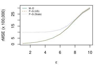
(a) Scenario #1: Same $n_{i}$; Same $\lambda_{i}$

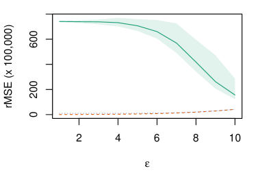
(b) Scenario #2: Different $n_{i}$; Same $\lambda_{i}$

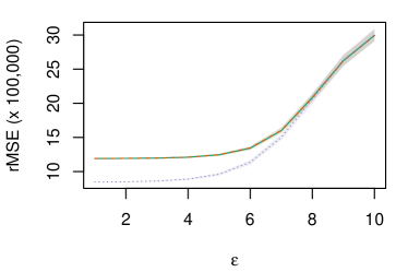
(c) Scenario #3: Same $n_{i}$; Different $\lambda_{i}$

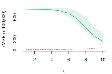
(d) Scenario #4: Different $n_{i}$; Different $\lambda_{i}$

Figure 1: Root mean square error from simulation study.

In retrospect, it is clear why this occurs. When all counties share the same population size, the multinomial-Dirichlet model with $\alpha_{i}=\alpha$ is mathematically equivalent to the Poisson-gamma model with $\lambda_{i}=y_{\cdot}/n_{\cdot}$ and $a_{i}=a$. To see why the multinomial-Dirichlet model performs poorly compared to the Poisson-gamma models when the population sizes vary, we look to the expected values for the synthetic data. Under the multinomial-Dirichlet approach from Section 2.1,

$$E\left[z_{i}\,|\,{\bf y},\mbox{\boldmath$\alpha$}\right] =E\left(E\left[z_{i}\,|\,\mbox{\boldmath$\theta$}\right]\,|\,{\bf y},\mbox{\boldmath$\alpha$}\right)=E\left[\theta_{i}z_{\cdot}\,|\,{\bf y},\mbox{\boldmath$\alpha$}\right]=\frac{y_{i}+\alpha_{i}}{\sum_{j}y_{j}+\alpha_{j}}z_{\cdot}\to\frac{\alpha_{i}}{\sum_{j}\alpha_{j}}z_{\cdot}=\frac{z_{\cdot}}{I};$$ (16)

i.e., as $\alpha_{i}\to\infty$, the events will become uniformly distributed among the $I$ counties. In contrast, if $z_{\cdot}=y_{\cdot}$ and $\sum_{j}n_{j}\lambda_{j}\approx y_{\cdot}$, the expected value for $z_{i}$ under the Poisson-gamma model from Section 2.2 yields

$$E\left[z_{i}\,|\,{\bf y},{\bf a},{\bf b}\right] =E\left(E\left[z_{i}\,|\,\mbox{\boldmath$\lambda$}\right]\,|\,{\bf y},{\bf a},{\bf b}\right)=E\left[\frac{n_{i}\lambda_{i}}{\sum_{j}n_{j}\lambda_{j}}z_{\cdot}\,|\,{\bf y},{\bf a},{\bf b}\right]\approx\frac{y_{i}+a_{i}}{n_{i}+b_{i}}n_{i}\to n_{i}\lambda_{0i};$$ (17)

i.e., as $a_{i},b_{i}\to\infty$, the events will be distributed in a manner which reflects the population sizes and prior event rates, $a_{i}/b_{i}=\lambda_{0i}$, of the counties. That is, when there is heterogeneity in the population sizes, we should expect the Poisson-gamma model to produce synthetic data with greater utility than the multinomial-Dirichlet model with an equivalent risk of disclosure. Furthermore, when we allow the model to use existing prior information regarding heterogeneity in the event rates, additional gains in utility should be expected.

To put these results in context, we consider the extent to which the urban-rural disparity and comparison of rates in New Mexico and New York can be distorted by the data synthesis process under Scenario 4. In Figure 2(a), we compare the heart disease mortality rate of urban counties to that from rural counties. Because there are far more rural counties than urban counties, the multinomial-Dirichlet model allocates a disproportionate number of deaths to rural counties, thus dramatically inflating their rates. In contrast, the Poisson-gamma model with smoothing toward state-specific averages produces rate estimates for both urban and rural counties that are on par with the truth. Similarly, Figure 2(b) displays a comparison of estimated rates for New York versus New Mexico. Because New York has 14 times the adult population of New Mexico and has only 2 times as many counties, the multinomial-Dirichlet model produces rate estimates for New Mexico that are approximately $14/2=7$ times greater than those in New York. This is again in contrast to the Poisson-gamma model with smoothing toward the state-specific averages, which (by design) produces accurate estimates for all $\epsilon$. Thus, while synthetic data produced by the Poisson-gamma model may yield more conservative inference (particularly when smoothing toward the national average), synthetic data from the multinomial-Dirichlet model may yield estimates that exhibit both Type-M (magnitude) and Type-S (sign) errors (Gelman and Tuerlinckx,, 2000).

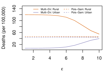
(a) Urban versus Rural

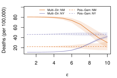
(b) New Mexico versus New York

Figure 2: Illustration of properties of the utility of the synthetic data. Synthetic data generated from the Poisson-gamma model are smoothed toward the state-specific averages.

4 Discussion

In this paper, we have generalized the approach of Machanavajjhala et al., (2008) for generating differentially private synthetic data from the multinomial-Dirichlet setting to a more flexible Poisson-gamma setting. In addition to decomposing a collection of abstract probability parameters into a function of interpretable offset (e.g., population size) and rate parameters, the Poisson-gamma setting also grants data stewards more control over the utility of the synthetic data. As we have demonstrated via simulation and proved mathematically, the Poisson-gamma approach can be equivalent to the multinomial-Dirichlet approach in the most simple of settings (equal population sizes and prior beliefs) while its added flexibility can yield far greater utility in more realistic settings.

One note that we have glossed over to this point is the notion that this approach assumes that (and conditions on) certain pieces of information are safe to be disclosed. In particular, we have assumed in our simulation study that the total number of deaths due to a certain cause of death in a particular age group is known (i.e., $y_{\cdot}$). This implies that we are comfortable with an intruder knowing that a given individual died of this cause of death at a certain age but not which county the individual lived in. In other settings, however, an agency may assume that demographic attributes such as an individual’s age, race, sex, and county are known, but that their cause of death is unknown. In this scenario, the presentation described here could simply be reframed to synthesize the number of individuals assigned to each ICD-10 code within these demographic strata – because the total number of deaths occurring in each strata would likely be small, differential privacy could be satisfied with relatively noninformative priors even for small $\epsilon$. This provides yet another lever for agencies to manipulate to improve the utility of the data they release.

Another avenue for improving the utility of the synthetic data produced by the proposed Poisson-gamma model would be to consider the $\left(\mbox{$\epsilon$},\delta\right)$-probabilistic differential privacy framework proposed by Machanavajjhala et al., (2008). As described in Section 2.1, satisfying $\epsilon$-differential privacy requires bounding the maximal risk, which occurs when $y_{i}=1$ in the true data and all $z_{\cdot}$ events are assigned to the $i$th cell in the synthetic data. Because the probability of sampling such an extreme synthetic dataset is very small, Machanavajjhala et al., (2008) proposed an algorithm for defining $\alpha$ such that the probability of sampling a synthetic dataset, ${\bf z}$, that violates (1) was less than a user-defined $\delta>0$. While it is possible to derive a similar framework for the Poisson-gamma model proposed here, we believe an approach that truncates the range of each $z_{i}$ based on its prior predictive distribution, $p\left(z_{i}\,|\,a_{i},b_{i}\right)$, could be more intuitive to implement and result in a true differentially private mechanism (i.e., $\delta=0$).

Finally, we would be remiss to not discuss the relationship between the proposed Poisson-gamma model and more conventional approaches for satisfying differential privacy — i.e., those that sanitize the truth by adding differentially private noise. In particular, one might suspect that such approaches would struggle when there is substantial heterogeneity in the counts because the impact of adding noise to $y_{i}=0$ events from a small $n_{i}$ is much different than adding the same amount of noise to a large $y_{i^{\prime}}$ out of a similarly large $n_{i^{\prime}}$ — i.e., the noise added is not itself a function of the number of events or the population size. One compromise might be the model-based differentially private synthesis (MODIPS) approach of Liu, (2016) in which posterior distributions are sanitized by adding differentially private noise to the sufficient statistics. In particular, the approach of Liu, (2016) could easily be extended to the Poisson-gamma setting in which the posterior distribution in (7) would be replaced by

$$\lambda_{i}^{*}\,|\,y_{i}\sim\mbox{$\text{Gamma}$}\left(a_{i}+f\left(y_{i}\right),b_{i}+n_{i}\right),$$ (18)

where $f\left(y_{i}\right)=y_{i}+e_{i}$ and $e_{i}$ is differentially private noise. While the $a_{i}+e_{i}$ in (18) will surely be less than the $a_{i}$ required to satisfy $\epsilon$-differential privacy in (15) — suggesting the potential for improved utility — the drawback of (18) is that $E\left[\lambda_{i}^{*}\,|\,y_{i}\right]=\left(a_{i}+y_{i}+e_{i}\right)/\left(b_{i}+n_{i}\right)$ is not a weighted average the crude rate from the data, $y_{i}/n_{i}$, and the prior expected value, $a_{i}/b_{i}$. As a result, the benefit of using less informative priors could potentially be negated by smoothing $\lambda_{i}^{*}$ toward $\left(a_{i}+e_{i}\right)/b_{i}$. Alternatively, we could sanitize the gamma prior in (6) itself. For instance, instead of smoothing the $\lambda_{i}$ toward their state-specific averages — $\lambda_{0;s_{i}}=\sum_{j\in{\cal S}_{s_{i}}}y_{j}/\sum_{j\in{\cal S}_{s_{i}}}n_{j}$, where ${\cal S}_{s}$ denotes the set of counties belonging to state $s$ — we could let $b_{i}^{*}=a_{i}/\lambda_{0;s_{i}}^{*}$ and $\lambda_{i}\sim\mbox{$\text{Gamma}$}\left(a_{i},b_{i}^{*}\right)$ where

$$\lambda_{0;s_{i}}^{*}=\frac{\sum_{j\in{\cal S}_{s_{i}}}y_{j}+e_{s_{i}}}{\sum_{j\in{\cal S}_{s_{i}}}n_{j}}$$ (19)

and $e_{s_{i}}$ is differentially private noise. A key benefit of this approach would be that the noise in (19) would be added to larger, aggregate counts, thereby resulting in less degradation to the utility of the model. Nevertheless, the focus of this paper is not to argue which approach is optimal (a status that is likely application specific), but rather to demonstrate the conditions in which the Poisson-gamma model satisfies differential privacy.

Issues with the utility of differentially private synthetic data are not new. In particular, Charest, (2010) highlighted the inherent bias in (16) for the multinomial-Dirichlet model due to the tendency to let $\alpha_{i}=\alpha$ for all $i$. That is, unlike in most Bayesian statistical approaches for generating synthetic data, prior distributions in differentially private synthesizers tend to be designed solely to satisfy differential privacy for a certain $\epsilon$ rather than represent one’s prior beliefs or best capture the data’s complex dependence structures. To overcome this bias, Charest, (2010) proposed what essentially amounts to a measurement error model in which the synthetic data are treated as a noisy version of the truth and the end-user attempts to estimate the truth from the synthetic data — i.e., make inference on $p\left({\bf y}\,|\,{\bf z},\mbox{\boldmath$\alpha$}\right)$. The drawback of this approach, however, is that it assumes (a) that end-users are aware of this bias, (b) that end-users are savvy enough to do such preprocessing of the public-use data, and (c) that agencies would disclose the details of their data synthesizers — including the level of $\epsilon$ used — to accurately recover or approximate the true data.

While such techniques can be effective for overcoming the bias induced by sanitizing data for public-use, the proposed work is intended as a step toward differentially private synthetic data that require no preprocessing on the part of would-be data users. Specifically, the Poisson-gamma model has parameters to control the informativeness of the model, ${\bf a}$, and parameters that dictate what the model smooths estimates toward, ${\bf b}$. As illustrated here, this framework allowed us to account for heterogeneity in both population sizes and prior event rates to yield synthetic data with substantially improved utility. In our future work, we aim to develop further extensions of formal privacy guarantees to nonconjugate models, thereby permitting the creation and dissemination of differentially private synthetic data that benefit from more conventional spatial and spatiotemporal model structures like those used by Quick and Waller, (2018). In the meantime, we believe that utility can be improved via truncating synthetic counts to reasonable ranges and stratification; e.g., synthesizing counts based on demographics such as age group, race/ethnicity, and sex and by geographic regions like the Census Regions and Divisions.

References

- Abowd, (2018) Abowd, J. M. (2018). “The U.S. Census Bureau adopts differential privacy.” In Proceedings of the 24th ACM SIGKDD International Conference on Knowledge Discovery and Data Mining, KDD ’18, 2867. New York, NY, USA: ACM.
- Apple Computer, (2017) Apple Computer (2017). “Differential Privacy.” https://www.apple.com/privacy/docs/Differential_Privacy_Overview.pdf.
- Besag et al., (1991) Besag, J., York, J., and Mollié, A. (1991). “Bayesian image restoration, with two applications in spatial statistics.” Annals of the Institute of Statistical Mathematics, 43, 1–59.
- Bowen and Liu, (2018) Bowen, C. M. and Liu, F. (2018). “Comparative study of differentially private data synthesis methods.” arXiv:1602.01063v3.
- Bradley et al., (2015) Bradley, J. R., Holan, S. H., and Wikle, C. K. (2015). “Multivariate spatio-temporal models for high-dimensional areal data with application to Longitudinal Employer-Household Dynamics.” Annals of Applied Statistics, 9, 1761–1791.
- Brillinger, (1986) Brillinger, D. R. (1986). “The natural variability of vital rates and associated statistics.” Biometrics, 42, 693–734.
- CDC, (2003) CDC (2003). “CDC/ATSDR Policy on Releasing and Sharing Data.” Manual; Guide CDC-02. Available at http://www.cdc.gov/maso/Policy/ReleasingData.pdf. Accessed June 30, 2015.
- CDC/NCHS, (2003) CDC/NCHS (2003). “Compressed Mortality File 1979-1998. CDC WONDER On-line Database, compiled from Compressed Mortality File CMF 1968-1988, Series 20, No. 2A, 2000 and CMF 1989-1998, Series 20, No. 2E, 2003.” https://wonder.cdc.gov/controller/saved/D16/D10F745. Accessed Mar 3, 2017.
- Charest, (2010) Charest, A.-S. (2010). “How can we analyze differentially-private synthetic datasets?” Journal of Privacy and Confidentiality, 2, 21–33.
- Clayton and Kaldor, (1987) Clayton, D. and Kaldor, J. (1987). “Empirical Bayes estimates of age-standardized relative risks for use in disease mapping.” Biometrics, 43, 671–681.
- Datta et al., (2017) Datta, A., Banerjee, S., and Hodges, J. S. (2017). “Spatial disease mapping using Directed Acyclic Graph Auto-Regressive (DAGAR) models.” ArXiv preprint 1704.07848.
- Ding et al., (2017) Ding, B., Kulkarni, J., and Yekhanin, S. (2017). “Collecting Telemetry Data Privately.” In Advances in Neural Information Processing Systems 30.
- Dinur and Nissim, (2003) Dinur, I. and Nissim, K. (2003). “Revealing information while preserving privacy.” In Proceedings of the Twenty-second ACM SIGMOD-SIGACT-SIGART Symposium on Principles of Database Systems, PODS ’03, 202–210. New York, NY, USA: ACM.
- Drechsler, (2011) Drechsler, J. (2011). Synthetic datasets for statistical disclosure control. Springer: New York.
- Dwork, (2006) Dwork, C. (2006). “Differential privacy.” In 33rd International Colloquium on Automata, Languages, and Programming, part II, 1–12. Berlin: Springer.
- Dwork et al., (2006) Dwork, C., McSherry, F., Nissim, K., and Smith, A. (2006). “Calibrating Noise to Sensitivity in Private Data Analysis.” In Theory of Cryptography, eds. S. Halevi and T. Rabin, 265–284. Berlin, Heidelberg: Springer.
- Erlingsson et al., (2014) Erlingsson, U., Pihur, V., and Korolova, A. (2014). “RAPPOR: Randomized aggregatable privacy-preserving ordinal response.” In Proceedings of the 2014 ACM SIGSAC Conference on Computer and Communications Security (CCS ’14), 1054–1067. New York, NY, USA: ACM.
- Garfinkel et al., (2018) Garfinkel, S. L., Abowd, J. M., and Powazek, S. (2018). “Issues encountered deploying differential privacy.” In Proceedings of the 2018 Workshop on Privacy in the Electronic Society, WPES’18, 133–137. New York, NY, USA: ACM.
- Gelfand and Vounatsou, (2003) Gelfand, A. E. and Vounatsou, P. (2003). “Proper multivariate conditional autoregressive models for spatial data analysis.” Biostatistics, 4, 11–25.
- Gelman and Tuerlinckx, (2000) Gelman, A. and Tuerlinckx, F. (2000). “Type S error rates for classical and Bayesian single and multiple comparison procedures.” Computational Statistics, 15, 373–390.
- Ghosh et al., (2012) Ghosh, A., Roughgarden, T., and Sundararajan, M. (2012). “Universally utility-maximizing privacy mechanisms.” SIAM Journal on Computing, 41, 1673–1693.
- Holan et al., (2010) Holan, S. H., Toth, D., Ferreira, M. A. R., and Karr, A. (2010). “Bayesian multiscale multiple imputation with implications for data confidentiality.” Journal of the American Statistical Association, 105, 564–577.
- Hu, (2018) Hu, J. (2018). “Bayesian estimation of attribute and identification disclosure risks in synthetic data.” ArXiv preprint, arXiv:1804.02784.
- Hu et al., (2018) Hu, J., Reiter, J. P., and Wang, Q. (2018). “Dirichlet process mixture models for modeling and generating synthetic versions of nested categorical data.” Bayesian Analysis, 13, 183–200.
- Little, (1993) Little, R. J. A. (1993). “Statistical analysis of masked data.” Journal of Official Statistics, 9, 407–426.
- Liu, (2016) Liu, F. (2016). “Model-based differentially private data synthesis.” ArXiv preprint, arXiv:1606.08052.
- Machanavajjhala et al., (2008) Machanavajjhala, A., Kifer, D., Abowd, J., Gehrke, J., and Vilhuber, L. (2008). “Privacy: Theory meets practice on the map.” In IEEE 24th International Conference on Data Engineering, 277–286.
- Manrique-Vallier and Hu, (2018) Manrique-Vallier, D. and Hu, J. (2018). “Bayesian non-parametric generation of synthetic multivariate categorical data in the presence of structural zeros.” Journal of the Royal Statistical Society, Series A, 181, 635–647.
- McSherry and Talwar, (2007) McSherry, F. and Talwar, K. (2007). “Mechanism Design via Differential Privacy.” In 48th Annual IEEE Symposium on Foundations of Computer Science (FOCS’07), 94–103.
- Quick et al., (2015) Quick, H., Holan, S. H., and Wikle, C. K. (2015). “Zeros and ones: A case for suppressing zeros in sensitive count data with an application to stroke mortality.” Stat, 4, 227–234.
- Quick et al., (2018) — (2018). “Generating partially synthetic geocoded public use data with decreased disclosure risk using differential smoothing.” Journal of the Royal Statistical Society, Series A, 181, 649–661.
- Quick and Waller, (2018) Quick, H. and Waller, L. A. (2018). “Using spatiotemporal models to generate synthetic data for public use.” Spatial and Spatio-Temporal Epidemiology, 27, 37–45.
- Quick et al., (2017) Quick, H., Waller, L. A., and Casper, M. (2017). “Multivariate spatiotemporal modeling of age-specific stroke mortality.” Annals of Applied Statistics, 11, 2170–2182.
- Raghunathan et al., (2003) Raghunathan, T. E., Reiter, J. P., and Rubin, D. B. (2003). “Multiple imputation for statistical disclosure limitation.” Journal of Official Statistics, 19, 1–16.
- Reiter, (2002) Reiter, J. P. (2002). “Satisfying disclosure restrictions with synthetic data sets.” Journal of Official Statistics, 18, 531–544.
- Reiter, (2003) — (2003). “Inference for partially synthetic, public use microdata sets.” Survey Methodology, 29, 181–188.
- Reiter, (2005) — (2005). “Using CART to generate partially synthetic, public use microdata.” Journal of Official Statistics, 21, 441–462.
- Reiter and Mitra, (2009) Reiter, J. P. and Mitra, R. (2009). “Estimating risks of identification disclosure in partially synthetic data.” Journal of Privacy and Confidentiality, 1, 99–110.
- Rubin, (1993) Rubin, D. B. (1993). “Satisfying confidentiality constraints through use of synthetic multiply-imputed microdata.” Journal of Official Statistics, 9, 461–468.
- Wasserman and Zhou, (2010) Wasserman, L. and Zhou, S. (2010). “A statistical framework for differential privacy.” Journal of the American Statistical Association, 105, 375–389.