Abstract

We have developed an accelerating cosmological model for the present universe which is phantom for the period $(0\leq z\leq 1.99)$ and quintessence phase for $(1.99\leq z\leq 2.0315)$. The universe is assumed to be filled with barotropic and dark energy(DE) perfect fluid in which DE interact with matter. For a deceleration parameter(DP) having decelerating-accelerating transition phase of universe, we assume hybrid expansion law for scale factor. The transition red shift for the model is obtained as $z_{t}=0.956$. The model satisfies current observational constraints.

1 Introduction

The cosmological principle (CP), which states that there is no privileged position in the universe and it is as such spatially homogeneous and isotropic, is the backbone of any cosmological model of the universe. Friedman-Lemaitre-Robertson-Walker (FLRW) line element fits best with the CP. The FLRW model, in the background of a perfect fluid distribution of matter, represents an expanding and decelerating universe. However the latest findings on observational grounds during the last three decades by various cosmological missions [1]$-$[17] all confirm that our universe is undergoing an accelerating expansion. In $\Lambda$CDM cosmology [18, 19], the $\Lambda$- term is used as a candidate of DE with equation of state $p_{\Lambda}=\rho_{\Lambda}=\frac{-\Lambda c^{4}}{8\pi G}$. However, the model suffers from, inter alia, fine tuning and cosmic coincidence problems [20]. Any acceptable cosmological model must explain the accelerating universe.

Of late, many authors [21]$-$[26] presented DE models in which the DE is considered in a conventional manner as a fluid with an EoS parameter $\omega_{de}=\frac{p_{de}}{\rho_{de}}$. It is assumed that our universe is filled with two types of perfect fluids in which one is a barotropic fluid (BF) which has positive pressure and creates deceleration in the universe. The other one is a DE fluid which has negative pressure and creates acceleration in the universe. Both fluids have different EoS parameters. Zhang and Liu [27] have constructed DE models with higher derivative terms. Liang et al. [28] have investigated two-fluid dialation model of DE. The modified Chaplygin gas with interaction between holographic DE and dark matter has been discussed by Wang et al. [29].

Recently, it has been discovered that the interaction between DE and dark matter(DM) offers an attractive alternative to the standard model of the cosmology [30, 31]. In these works the motivation to study interacting DE model arises from high energy physics. In recent work Risalti and Lusso [32] and Riess et al. [33] stated that a rigid $\Lambda$ is ruled out by $~{}4\sigma$ and allowing for running vacuum favored phantom type DE ($\omega<-1$) and $\Lambda$ CDM is claimed to be ruled out by $4.4\sigma$ motivating the study of interactive DE models. Interacting DE models [34]$-$[38] lead to the idea that DE and DM do not evolve separately but interact with each other non gravitationally (see recent review [39] and references there in.).

In this paper, we have developed an accelerating cosmological model for the present universe which is phantom for the period $(0\leq z\leq 1.99)$ and quintessence phase for $(1.99\leq z\leq 2.0315)$. The universe is assumed to be filled with barotropic and dark energy(DE) perfect fluid in which DE interact with matter. For a deceleration parameter(DP) having decelerating-accelerating transition phase of universe, we assume hybrid expansion law for scale factor. The transition red shift for the model is obtained as $z_{t}=0.956$. The model satisfies current observational constraints.

2 Basic field equations

The dynamics of the universe is governed by the Einstein’s field equations (EFEs) given by

$$R_{ij}-\frac{1}{2}Rg_{ij}=-\frac{8\pi G}{c^{4}}T_{ij},$$ (1)

where $R_{ij}$ is the Ricci tensor, $R$ is the scalar curvature, and $T_{ij}$ is the stress-energy tensor taken as $T_{ij}=T_{ij}(m)+T_{ij}(de).$ We assume that our universe is filled with two types of perfect fluids (since homogeneity and isotropy imply that there is no bulk energy transport), namely baryonic fluid and dark energy. The energy-momentum tensors of the contents of the universe are presented as follows: ( The subscripts $m$ and $de$ denote ordinary matter and dark energy, respectively.) $T_{ij}(m)=\left(\rho_{m}+p_{m}\right)u_{i}u_{j}-p_{m}g_{ij}$ and $T_{ij}(de)=\left(\rho_{de}+p_{de}\right)u_{i}u_{j}-p_{de}g_{ij}$. In standard spherical coordinates $x^{i}=(t,r,\theta,\phi)$, a spatially homogeneous and isotropic FLRW line-element is the following (in units $c=1$)

$$ds{}^{2}=dt{}^{2}-a(t){}^{2}\left[\frac{dr{}^{2}}{(1+kr^{2})}+r^{2}({d\theta{}^{2}+sin{}^{2}\theta d\phi{}^{2}})\right],$$ (2)

where (i) k=-1 is closed universe (ii) k=1 is open universe and (iii) k=0 is spatially flat universe. Solving EFEs (1) for the FRW metric (2), we get the following equations of dynamic cosmology.

$$2\frac{\ddot{a}}{a}+H^{2}=-8\pi Gp+\frac{k}{a^{2}}$$ (3)

and

$$H^{2}=\frac{8\pi G}{3}\rho+\frac{k}{a^{2}},$$ (4)

where $H=\frac{\dot{a}}{a}$ is the Hubble constant. Here an over dot means differentiation with respect to cosmological time $t$. We have deliberately put the curvature term on the right of Eqs. (3) and (4), as this term is made to acts like an energy term. For this, we assume that the density and pressure for the curvature energy are as follows $\rho_{k}=\frac{3k}{8\pi Ga^{2}},p_{k}=-\frac{k}{8\pi Ga^{2}}.$ With this choice, Eqs. (3) and (4) are read as

$$2\frac{\ddot{a}}{a}+H^{2}=-8\pi G(p+p_{k})$$ (5)

and

$$H^{2}=\frac{8\pi G}{3}\,(\rho+\rho_{k}).$$ (6)

The energy density $\rho$ in Eq. (6) is comprised of two types of energy, namely matter and dark energy $\rho_{m}$ and $\rho_{de}$, where as the pressure ‘$p$’ in Eq. (5) is comprised of pressure due to matter and pressure due to dark energy. We can express $\rho=\rho_{m}+\rho_{de}$ and $p=p_{m}+p_{de}.$

3 Energy conservation laws & densities

The energy conservation law[ECL]  $T^{ij}_{;j}=0$  provides the following well known equation amongst the density $\rho$, pressure $p$ and Hubble constant $H$, $\dot{\rho}+3H(p+\rho)=0$, where $\rho=\rho_{m}+\rho_{de}+\rho_{k}$ and $p=p_{m}+p_{de}+p_{k},$ are the total density and pressure of the universe, respectively. We see that $\rho_{k}$ and $p_{k}$ satisfy ECL independently, i.e.$\dot{\rho_{k}}+3H(p_{k}+\rho_{k})=0$, so that $\frac{d}{dt}{(\rho_{m}+\rho_{de})}+3H(p_{m}+p_{de}+\rho_{m}+\rho_{de})=0$. We assume that DE interacts with and transforms energy to baryonic matter. For this, the continuity equations for the dark and baryonic fluids can be written as follows

$$\dot{\rho_{m}}+3H(p_{m}+\rho_{m})=Q$$ (7)

and

$$\dot{\rho_{de}}+3H(p_{de}+\rho_{de})=-Q$$ (8)

The quantity Q represents the energy transfer from DE to baryonic matter, so we take $Q\geq 0$. We follow Amendola el al. [40] and Gou el al. [41], to assume that

$$Q=3H\sigma\rho_{m},$$ (9)

where $\sigma$ is a coupling constant and is positive.

At present our universe is dust filled, so we take $p_{m}=0$. Integrating Eqs. (7) and (8) with the help of Eq. (9), we get $\rho_{m}=(\rho_{m})_{0}\left(1+z\right)^{3(1-\sigma)}$ and $\rho_{de}=(\rho_{de})_{0}~{}exp\left(3\int^{z}_{0}\frac{(1+\omega_{de})dz}{1+z}\right)$, where we have put $\frac{a_{0}}{a}=1+z$. Clearly DE helps in the expansion of the universe through energy transfer. The EoS for the curvature energy is obtained as $p_{k}=\omega_{k}\rho_{k}~{}\mbox{where}~{}\omega_{k}=-1/3.$ This gives $\rho_{k}=(\rho_{k})_{0}(1+z)^{2}.$ The critical density and density parameters for energy density, dark energy and curvature density are, respectively, defined by $\rho_{c}=\frac{3H^{2}}{8\pi G},\Omega_{m}=\frac{\rho_{m}}{\rho_{c}},\Omega_{de}=\frac{\rho_{de}}{\rho_{c}}$ and $\Omega_{k}=\frac{\rho_{k}}{\rho_{c}}$, where $\rho_{c}$, $\Omega_{m}$, $\Omega_{de}$ and $\Omega_{k}$ are the critical density, matter energy , dark energy and curvature energy parameters respectively.

With these in hand, we can write the FRW field equations as follows

$$H^{2}=H^{2}_{0}\left[(\Omega_{m})_{0}\left(1+z\right)^{3(1-\sigma)}+(\Omega_{k})_{0}\left(1+z\right)^{2}\right]+H^{2}\Omega_{de},$$ (10)

and

$$2q=1-\frac{H^{2}_{0}}{H^{2}}(\Omega_{k})_{0}\left(\frac{a_{0}}{a}\right)^{2}+3\omega_{de}\Omega_{de},$$ (11)

where $q$ is DP defined by $q=-\frac{\ddot{a}}{aH^{2}}.$ The purpose of this paper is to investigate the evolution of $\omega_{de}$ over red shift or time and to match it with the observational constraint.

4 Hybrid Scale Factor with Plank Results

We have only two equations and the scale factor ‘$a$’, pressure $p$ and energy density $\rho$ to be determined. So we have to use a certain ansatz. As motivation for the ansatz, we note some important solutions. The De Sitter universe has scale factor $a(t)=exp(\Lambda t)$ where $\Lambda$ is the positive cosmological. Later on, FRW cosmological models were proposed in which Einstein and De Sitter gave the power law expansion law $a(t)=t^{2/3}$ for flat space-time. Off late, during the last three decades, researchers are working with accelerating expanding models describe a transition from deceleration to acceleration.

In the literature a constant deceleration parameter [42]$-$[45] and references therein, has been used to give a power or exponential law. As it has been discussed in the introduction that in view of the recent observations of Type Ia supernova [1]$-$[5], WMAP collaboration [12, 46, 47], and Planck Collaboration [17] there is a need of a time-dependent deceleration parameter which describe decelerated expansion in the past and accelerating expansion at present, so there must be a transition from deceleration to acceleration. The deceleration parameter must show the change in signature [48]$-$[50].

Now, we consider a well-motivated ansatz considered by Abdussattar and Prajapati [51], which puts a constraint on the functional form of the deceleration parameter $q$ as

$$q=\frac{kn}{(k+t)^{2}}-1,$$ (12)

where $k>0$ (dimension of square of time) and $n>0$ (dimensionless) are constants. For such choice of the scale factor, we see that $q=0$ when $t=\sqrt{kn}-k$. We get $q>0$ (i.e. decelerated expansion) for $t<\sqrt{kn}-k$ and $q<0$ (i.e. accelerated expansion) for $t>\sqrt{kn}-k$. Integrating $q=-\frac{\ddot{a}a}{\dot{a}^{2}}$, we find the scale factor as

$$a(t)=c_{2}\exp\int\frac{dt}{\int(1+q)dt+c_{1}},$$ (13)

where $c_{1},c_{2}$ are integrating constants.

Choosing appropriate values of the constants ($c_{1}=n$ and $c_{2}=1$), one can integrate Eq. (13) with the help Eq. (12) to get the scale factor as

$$a(t)=t^{\alpha}\exp(\beta t),$$ (14)

where $\alpha>0$ and $\beta>0$ are constants.

Akarsu et al. [52] also used hybrid expansion law [HEL] with scalar field reconstruction of observational constraints and cosmic history. Avil$e^{\prime}$s et al. [53] used HEL with integrating cosmic fluid. Several authors [54]$-$[61] have considered the HEL for solving different cosmological problems in general relativity and $f(R,T)$ gravity theories. Some work is done by Moraes [62] and Moraes et al. [63]. Recently, Moraes and Sahoo [64] investigated non-minimal matter geometry coupling in the $f(R,T)$ gravity by using HEL.

The hybrid scale factor has a transition behavior from deceleration to acceleration. Capozziello et al. [65] studied the cosmographic bounds on cosmological deceleration-acceleration transition red shift in $f(R)$ gravity. The author considered a Tailor expansion of $f(z)$ in term of $a(t)=\frac{1}{1+z}$ which for Friedmann equations, comes in the range $z\leq 2.$ Capozziello et al. [66] also extracts constraints on the transition red shift $z_{tr}$ in the frame work of $f(T)$ gravity which becomes compatible with the constraints predicted by $\Lambda$ CDM model at the 1-$\sigma$ confidence level. Their [66] values seems to be slightly smaller than theoretical expectation, i.e., $z_{tr}=0.74$ according to [67]. Recently, Farooq et al. [68] compile updated list of $38$ measurements of Hubble parameter $H(z)$ between red shifts $0\leq z\leq 2.36$ and used them to put constraints on model parameters of constant and time-varying DE cosmological models, both spatially flat and curved.

Now we will determine the constants $\alpha$ and $\beta$ on the basis of the latest observational findings due to Planck [17]. The values of the cosmological parameters at present are as follows. $(\Omega_{m})_{0}$= 0.30 $(\Omega_{k})_{0}=\pm 0.005$, $(\omega_{de})_{0}=-1$, $(\Omega_{de})_{0}=0.70\pm 0.005$, $H_{0}=0.07$ Gyr^-1 and present age $t_{0}=13.72$ Gyr.

Using these values in Eq. (11), we get the present value of the deceleration parameter as $q_{0}\simeq 0.55$. From Eq. (14), we get following

$$\alpha(1+z)HH_{z}=\alpha(q+1)H^{2}=(H-\beta)^{2}=\frac{\alpha^{2}}{t^{2}},$$ (15)

where we have used $\dot{z}=-(1+z)H$ and $H_{z}$ means differentiation w.r.t. z. From Eq. (15) and Planck’s results, we get the value of constants $\alpha$ and $\beta$ as $\beta=0.0397474\sim 0.04,\alpha=0.415066\sim 0.415$.

5 Physical Properties of the model

5.1 Hubble Constant $H$

The determination of the two physical quantities $H_{0}$ and $q$ play an important role to describe the evolution of the universe. $H_{0}$ provides us the rate of expansion of the universe which in turn helps in estimating the age of the universe, whereas the deceleration parameter $q$ describes the decelerating or accelerating phases during the evolution of the universe. From the last two decades, many attempts [68]$-$[74] have been made to estimate the value of the Hubble constant as $H_{0}=72\pm 8kms^{-1}Mpc^{-1},~{}~{}69.7^{+4.9}_{-5.0}kms^{-1}Mpc^{-1},~{}~{}71\pm 2.5kms^{-1}Mpc^{-1},~{}~{}70.4^{+1.3}_{-1.4}kms^{-1}Mpc^{-1},~{}~{}73.8\pm 2.4kms^{-1}Mpc^{-1}and~{}~{}67\pm 3.2kms^{-1}Mpc^{-1}$ respectively. For detail discussions readers are referred to Kumar and more latest Farook [74, 68].

The exact solution of Eq. (15) is obtained for the Hubble constant $H$ as a function of redshift $z$ as follows

$$(H-\beta)^{\alpha}=A~{}\exp\left(\frac{\alpha\beta}{H-\beta}\right)(1+z),$$ (16)

where the constant of integration A is obtained as $A=0.134$ on the basis of the present value of $H(H_{0}=0.07$ Gy${}^{-1})$. A numerical solution of Eq. (16) shows that the Hubble constant is an increasing function of red shift. We present the following figures (1) and (2) to illustrate the solution.

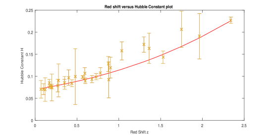
Figure 1: Plot of Hubble constant ($H$) versus redshift ($z$)

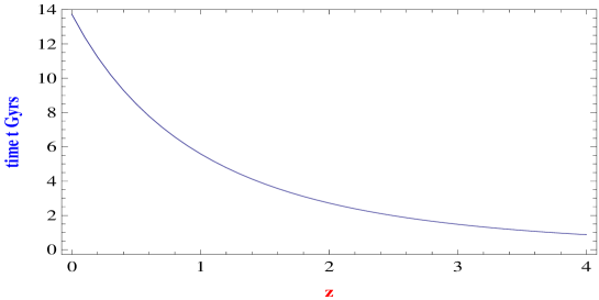
Figure 2: Variation of ($z$) versus ($t$)

As is clear from the figures, the Hubble constant varies slowly over red shift and time. Various researchers [75]$-$[80] have estimated values of the Hubble constant at different red-shifts using a differential age approach and galaxy clustering method. They have described various observed values of the Hubble constant $H_{ob}$ along with corrections in the range $0\leq z\leq 2$. It is found that both observed and theoretical values tally considerably and support our model.

In this figure $1$, cross signs are $31$ observed values of the Hubble constant $H_{ob}$ with corrections, whereas the linear curve is the theoretical graph of the Hubble constant $H$ as per our model. Figure $2$ is obtained from equation $\dot{z}=-(1+z)H(z)$. It plots the variation of redshift $z$ with time $t$, which shows that in the early universe the redshift was more than at present. From this figure, we can convert redshift into time.

5.2 Transition from Deceleration to Acceleration

Now we can obtain the deceleration parameter ’$q$’ in term of red shift ’$z$’ by using Eqs. (15) and (16). We present the following figure (3) to illustrate the solution. This describes the transition from deceleration to acceleration.

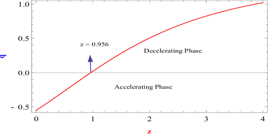
Figure 3: Variation of $q$ with $z$.

At $z=0.9557,~{}\&~{}0.9558$, our model gives following values of Hubble constant $H$, deceleration parameter $q$ and and corresponding time.

$$H(0.9557)\to 0.111206,~{}~{}q(0.9557)\to-0.0000124355,~{}~{}t(0.9557)\to 5.81124,$$

and

$$H(0.9558)\to 0.111212,~{}~{}q(0.9558)\to 0.0000450098,~{}~{}t(0.9558)\to 5.81078.$$

This means that the acceleration had begun at $z\to 0.95575,t\to 5.81104~{}Gyr,H\to 0.111209~{}Gyr^{-1}$.

5.3 DE Parameter $\Omega_{de}$ and EoS $\omega_{de}$

Now, from Eqs. (10),(11) and (16), the density parameter $\Omega_{de}$ and EoS parameter $\omega_{de}$ for DE are given by the following equations and are solved numerically.

$$H^{2}\Omega_{de}=H^{2}-(\Omega_{m})_{0}H^{2}_{0}(1+z)^{3(1-\sigma)}$$ (17)

and

$$\omega_{de}=\frac{(2-3\alpha)H^{2}-4\beta H+2\beta^{2}}{3\alpha[H^{2}-H_{0}^{2}(\Omega_{m})_{0}(1+z)^{3(1-\sigma)}]},$$ (18)

where we have taken $(\Omega_{k})_{0}=0$ for the present dust filled spatially flat universe. We would take $\sigma$ = 0.04 for numerical solutions to match with latest observations. We solve Eqs. (17) and (18) with the help of Eq. (16) and present following figures $3$ and $4$ to illustrate the solution.

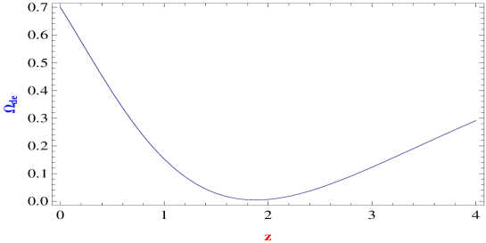
Figure 4: Plot of $\Omega_{de}$ versus redshift ($z$)

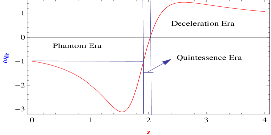
Figure 5: Plot of $\omega_{de}$ versus $z$. Phantom phase $(0\leq z\leq 1.99)$, quintessence phase $1.99\leq z\leq 2.0315$ and deceleration phase $z\geq 1.99$

Our model envisages that at present we are living in a phantom phase $\omega_{(de)}\leq-1$. In the past at $z=1.549~{}~{}\omega_{(de)}=-3.12191$ was minimum, then it started increasing. This phase remains for the period $(0\leq z\leq 1.99)$. Our universe entered into a quintessence phase at $z=1.99$, where $\omega_{de}$ comes up to $-0.333123$. As per our model, the period for the quintessence phase is the following

$$1.99\leq z\leq 2.0315.$$

DE favors deceleration at $z\geq 1.99$. The recent supernovae SNI $997ff$ at $z\simeq 1.7$ is consistent with a decelerated expansion at the epoch of high emission [72, 79, 80].

As per our model, the present value of DE is 0.7. It decreases over the past, attains a minimum value $\Omega_{de}=0.0368568$ at $z=1.834$, and then it again increases with red shift. The dark energy density is approximately 29% at red shift 4. Since dark energy density is significant at this red shift, it might have strong implications on structure formation, but at $z=4$, EoS parameter $\omega_{de}=1.0532$ is positive, so it will favor deceleration and hence structure formation.

5.4 Luminosity Distance

The redshift-luminosity distance relation [81] ia an important observational tool to study the evolution of the universe. The expression for the luminosity distance ($D_{L}$) is obtained in term of red-shift as the light coming out of a distant luminous body gets red shifted due to the expansion of the universe. We determine the flux of a source with the help of luminosity distance. It is given as

$$D_{L}=a_{0}r(1+z),$$ (19)

where r is the radial co ordinate of the source. In [18], $D_{L}$ is obtained as

$$D_{L}=\frac{c(1+z)}{H_{0}}\int^{z}_{0}\frac{dz}{h(z)},~{}h(z)=\frac{H}{H_{0}}$$ (20)

5.5 Distance modulus $\mu$ and Apparent Magnitude $m_{b}$

The distance modulus $\mu$ is derived as [18]

$$\mu = m_{b}-M$$

$$= 5log_{10}\left(\frac{D_{L}}{Mpc}\right)+25$$

$$= 25+5log_{10}\left[\frac{c(1+z)}{H_{0}}\int^{z}_{0}\frac{dz}{h(z)}\right].$$

(21)

The absolute magnitude $M$ of a supernova [18] is $M=16.08-25+5log_{10}(H_{0}/.026c)$, so we get following expression for the apparent magnitude $m_{b}$

$$m_{b}=16.08+5log_{10}\left[\frac{1+z}{.026}\int^{z}_{0}\frac{dz}{h(z)}\right].$$ (22)

We solve Eqs. (20), (21) and (22) with the help of Eq. (15). Our theoretical results have been compared with SNe Ia related $581$ data’s from Pantheon compilation [82] with possible error in the range ($0\leq z\leq 1.4$) and the derived model was found to be in good agreement with current observational constraints. The following Figures $6$ & $7$ depict the closeness of observational and theoretical results, thereby justifying our model.

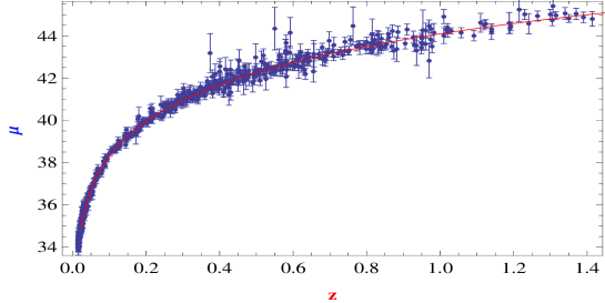
Figure 6: Plot of distance modulus ($\mu$) versus red-shift ($z$). Crosses are SNe Ia related $581$ data’s from Pantheon compilation with possible error.

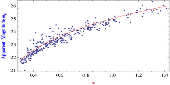
Figure 7: Plot of apparent magnitude ($m_{b}$) versus red-shift ($z$), Dots are SNe Ia related $287$ data’s from Pantheon compilation.

6 Conclusions

In this work, efforts were made to develop a cosmological model which satisfies the cosmological principle and incorporates the latest developments which envisaged that our universe is accelerating due to DE. We have also proposed a variable equation of state for DE in our model. We studied a model with dust and dark energy which shows a transition from deceleration to acceleration. We have successfully subjected our model to various observational tests. The main findings of our model are itemized point-wise as follows.

• The expansion of the universe is governed by a hybrid expansion law $a(t)=t^{\alpha}\exp(\beta t)$, where $\alpha=0.415,\beta=0.04$. This describes the transition from deceleration to acceleration.

• Our model is based on the latest observational findings due to the Planck results [17]. The model agrees with present cosmological parameters.
  $(\Omega_{m})_{0}$= 0.30 $(\Omega_{k})_{0}=\pm 0.005$, $(\omega_{de})_{0}=-1$, $(\Omega_{de})_{0}=0.70\pm 0.005$, $H_{0}=0.07$ Gy^-1, $q_{0}=0.055$ and present age $t_{0}=13.72$ Gy.

• Our model has a variable equation of states $\omega_{de}$ for the DE density. Our model envisage that at present we are living in the phantom phase $\omega_{(de)}\leq-1$. In the past at $z=1.549~{}~{}\omega_{(de)}=-3.12191$ was minimum, then it started increasing. This phase remains for the period $(0\leq z\leq 1.99)$. Our universe entered into a quintessence phase at $z=1.99$ where $\omega_{de}$ comes up to $-0.333123$. As per our model, the period for the quintessence phase is the following

  $$1.99\leq z\leq 2.0315$$

  . DE favors deceleration at $z\geq 1.99$.

• As per our model, the present value of DE is 0.7. It decreases over the past, attains a minimum value $\Omega_{de}=0.0368568$ at $z=1.834$, and then it again increases with red shift.

• We have calculated the time at which acceleration had begun. The acceleration had begun at $z\to 0.95575,t\to 5.81104~{}Gyr,H\to 0.111209~{}Gyr^{-1}$. At this time $\Omega_{de}=0.220369$ and $\omega_{de}=-1.54715$

References

- [1] S. Perlmutter et al., Nature 391, 51 (1998).
- [2] S. Perlmutter et al., Astrophys. J. 517, 5 (1999).
- [3] A. G. Riess et al., Astron. J. 116, 1009 (1998).
- [4] J. L. Tonry et al., Astrophys. J. 594, 1 (2003).
- [5] A. Clocchiatti et al., Astrophys. J. 642, 1 (2006).
- [6] P. de Bernardis et al., Nature 404, 955 (2000).
- [7] S. Hanany et al., Astrophys. J. 493, L53 (2000).
- [8] D. N. Spergel et al., Astrophys. J. Suppl. 148, 175 (2003).
- [9] M. Tegmark et al, Phys. Rev. D 69, 103501 (2004).
- [10] U. Seljak et al., Phys. Rev. D 71, 103515 (2005).
- [11] J. K. Adelman-McCarthy et al., Astrophys. J. Suppl. 162, 38 (2006).
- [12] C. L. Bennett et al., Astrophys. J. Suppl. 148 1 (2003).
- [13] S. W. Allen et al., Mon. Not. R. Astron. Soc. 353, 457 (2004).
- [14] N. Suzuki et al., Astrophys. J. 746, 85 (2011).
- [15] T. Delubac et al., Astron. Astrophys. 574, A59 (2015).
- [16] C. Blake et al., Mon. Not. R. Astron. Soc. 425, 405 (2012).
- [17] P. A. R. Ade et al., Astron. Astrophys. 594. A14 (2016).
- [18] E. J. Copeland et al., Int. J. Mod. Phys. D 15, 1753 (2006).
- [19] Grn and S. Hervik, Einstein’s general theory of relativity with modern applications in cosmology, Springer Publication, (2007).
- [20] S. Weinberg, Rev. Mod. Phys. 61, 1 (1989).
- [21] H. Amirhashchi, A. Pradhan and B. Saha, Chin. Phys. Lett. 28 039801(2011).
- [22] H. Amirhashchi ,A. Pradhan and H. Zainuddin, Int. J. Theor. Phys. 50, 3529( 2011)
- [23] A. Pradhan , H. Amirhashchi and B. Saha, Astrophys. Space Sci. 333, 343(2011)
- [24] B. Saha, H. Amirhashch and A. Pradhan, Astrophys. Space Sci. 342, 257(2012)
- [25] A. Pradhan, Indian J. Phys. 88, 215( 2014)
- [26] S. Kumar, Astrophys. Space Sci. 332, 449(2011)
- [27] X.F. Zhang and H. H. Liu, Chin. Phys. Lett. 26, 109803 ( 2009)
- [28] N. M. Liang, C.J. Gao and S.N. Zhang, Chin. Phys. Lett. 26, 069501( 2009)
- [29] C. Wang, Y.B. Wu and F. Liu, Chin. Phys. Lett. 26, 029801(2009)
- [30] J. Sola and A. Gomej-Valent, Int. J. Mod. Phys. D 24, 1541003 ( 2015)
- [31] D. Begue, C. Stahl and S. S. Xue, Nuec. Phys. B 940, 312(2019 )
- [32] G. Risaliti and E. Lusso, Nat. Astron. 3, 272(2019)
- [33] A.G. Riess et al., arXiv:1903.07603[astro-ph.CO]
- [34] S. S. Xue, Nucl. Phys B 897, 326( 2015)
- [35] E.G.M. Ferriera, Phys. Rev. D 95, 043520( 2017)
- [36] T. S. Koivisto, E.N. Saridakis and N. Tamanini, JCAP 1509, 047( 2015)
- [37] S. Kumar and R.C. Nunes, Phys. Rev. D 94, 123511(2016 )
- [38] S. Kumar and R.C. Nunes, Phys. Rev. D 96, 103511( 2017)
- [39] B. Wang, E. Abdulla , F. Atrio-Varandela and D. Pavon, Rept. Prog. Phys 79, 096901(2016).
- [40] L. Amendola, G. Camargo Campos, and R. Rosenfeld, Phys. Rev. D75, 083506(2007).
- [41] Z. K. Guo, N. Ohta, and S. Tsujikawa, Phys. Rev. D 76, 023508(2007).
- [42] M.S. Berman, II Nuovo Cimento B74, 1971( 1983).
- [43] M.S. Berman, F.M.Gomide, Gen. Relativ. Gravit. 20, 191(1988).
- [44] A. Pradhan , H. Amirhashchi and B. Saha , Int. J. Theor. Phys. 50, 2923(2011).
- [45] A. Pradhan, Commun. Theor. Phys. 55, 931(2011).
- [46] D.N. Spergel, et al., Astrophys. Jour. Suppl. 170, 377(2007).
- [47] D.Komatsu, et al., Astrophys. Jour. Suppl. Series. 180, 330( 2009).
- [48] T. Padmanabhan, T.R. Choudhury, Mon. Not. R. Astron. Soc. 244, 823(2003).
- [49] L. Amendola, Mon. Not. R. Astron. Soc. 342, 221(2003).
- [50] A. G. Riess, et al., Astrophys. J. Astrophys. 560, 49( 2001).
- [51] Abdusattar and S.R. Prajapati, Astrophys. Space Sci. 335, 657(2011).
- [52] O. Akarsu, et al., Jour. Cosm. Astrop. Phy. 01, 022(2014).
- [53] L. Avils, et al., Journ. Phys.: Conference series 70 , 012010( 2016).
- [54] S. Kumar, Grav. & Cosm. 19, 284-287(2013).
- [55] A. Pradhan and R. Jaisaval, Int. J. Geom. Methods Mod. Phys. 15, 1850076(2018).
- [56] C.R. Mahanta and N. Sharma, New Astronomy 57, 70(2017).
- [57] A.K. Yadav, et al., Int. J. Theor. Phys. 54, 1671-1679(2015).
- [58] R. Zia, D.C. Maurya and A. Pradhan, Int. J. Geom. Methods Mod. Phys. 15, 1850168(2018).
- [59] A.K. Yadav and V. Bhardwaj, Res. Astron. Astrophys. 18, 64(2016).
- [60] B. Mishra and S.K. Tripathi, Mod. Phys. A 30, 1550175(2015).
- [61] U.K. Sharma, et al., J. Astrophys. Astr. 40, 2(2019).
- [62] P.H.R.S. Moraes, Astrophys. Space Sci. 352, 273-279(2014).
- [63] P.H.R.S. Moraes, G.Ribeiro and R.A.C. Correa, Astrophys. Space Sci. 361, 227( 2016).
- [64] P.H.R.S. Moraes and P.K. Sahoo, Eur. Phys. J. C 77, 480(2017).
- [65] S. Capozziello, et al., Phys. Rev. D 90, 044016( 2014).
- [66] S. Capozziello, et al., Phys. Rev. D 91, 124037( 2015).
- [67] O. Farooq and B.Ratra, Astrophys. J. 766, L7(2013).
- [68] O. Farooq, et al., Astrophys. J. 835, 26 (2017)
- [69] W L Freedman et al, Astrophys. Journ., 553, 47 (2001).
- [70] S H Suyu et al, Astrophys. Jour. 711, 201 (2010).
- [71] N. Jarosik et al, Astrophys. Journ. Suppl. 192, 14 (2010).
- [72] A G Riess et al, Astrophys. Journ., 730, 119 (2011).
- [73] F Beutler et al, Mon. Not. R. Astron. Soc., 416, 3017 (2011).
- [74] S Kumar, Mon. Not. Astron. Soc., 422, 2532 (2012).
- [75] C Zhang et al, Res. Astron. Astrophys., 14, 1 (2014).
- [76] D Stern et al, Jour. Cosmo. Astropart. Phys., 1002, 008 (2010)
- [77] M Moresco, Mon. Not. R. Astron. Soc. 450, L16 (2015).
- [78] J Simon et al, Phys. Rev. D, 71, 123001 (2005).
- [79] N Benitez et al, Astrophys. Jour., 577, L1 (2002).
- [80] M. Turner and A G Riess, Astrophys. Jour., 569, 18 (2002).
- [81] A.R. Liddle and D.H. Lyth Cosmological Inflation and Large-Scale Structure (Cambridge University Press 2000)
- [82] D. M. Scolnic, Astrophys. J. 859, 101(2018).