Deep Unknown Intent Detection with Margin Loss

Abstract

Identifying the unknown (novel) user intents that have never appeared in the training set is a challenging task in the dialogue system. In this paper, we present a two-stage method for detecting unknown intents. We use bidirectional long short-term memory (BiLSTM) network with the margin loss as the feature extractor. With margin loss, we can learn discriminative deep features by forcing the network to maximize inter-class variance and to minimize intra-class variance. Then, we feed the feature vectors to the density-based novelty detection algorithm, local outlier factor (LOF), to detect unknown intents. Experiments on two benchmark datasets show that our method can yield consistent improvements compared with the baseline methods.

1 Introduction

In the dialogue system, it is essential to identify the unknown intents that have never appeared in the training set. We can use those unknown intents to discover potential business opportunities. Besides, it can provide guidance for developers and accelerate the system development process. However, it is also a challenging task. On the one hand, it is often difficult to obtain prior knowledge about unknown intents due to lack of examples. On the other hand, it is hard to estimate the exact number of unknown intents. In addition, since user intents are strongly guided by prior knowledge and context, modeling high-level semantic concepts of intent is still problematic.

Few previous studies are related to unknown intents detection. For example, Kim and Kim (2018) try to optimize the intent classifier and out-of-domain detector jointly, but out-of-domain samples are still needed. The generative method Yu et al. (2017) try to generate positive and negative examples from known classes by using adversarial learning to augment training data. However, the method does not work well in the discrete data space like text, and a recent study Nalisnick et al. (2019) suggests that this approach may not work well on real-world data. Brychcin and Král try to model intents through clustering. Still, it does not make good use of prior knowledge provided by known intents, and clustering results are usually unsatisfactory.

Although there is a lack of prior knowledge about unknown intents, we can still leverage the advantage of known label information. Scheirer et al. (2013); Fei and Liu (2016) suggest that a m-class classifier should be able to reject examples from unknown class while performing m-class classification tasks. The reason is that not all test classes have appeared in the training set, which forms a (m+1)-class classification problem where the (m+1)^th class represents the unknown class. This task is called open-world classification problem. The main idea is that if an example dissimilar to any of known intents, it is considered as the unknown. In this case, we use known intents as prior knowledge to detect unknown intents and simplify the problem by grouping unknown intents into a single class.

Bendale and Boult (2016) further extend the idea to deep neural networks (DNNs). Shu et al. (2017) achieve the state-of-the-art performance by replacing the softmax layer of convolution neural network (CNN) with a 1-vs-rest layer consist of sigmoid and tightening the decision threshold of probability output for detection.

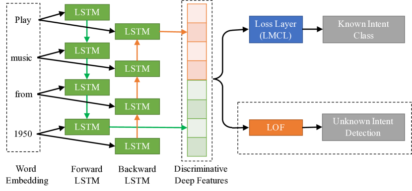
Figure 1: The architecture of the proposed two-stage method. We acquire intent representation by training an intent classifier on known intent with BiLSTM and learn discriminative deep features through LMCL. Then, we use LOF to detect unknown intents during the testing stage.

DNN such as BiLSTM Goo et al. (2018); Wang et al. (2018c) has demonstrated the ability to learn high-level semantic features of intents. Nevertheless, it is still challenging to detect unknown intents when they are semantically similar to known intents. The reason is that softmax loss only focuses on whether the sample is correctly classified, and does not require intra-class compactness and inter-class separation. Therefore, we replace softmax loss with margin loss to learn more discriminative deep features.

The approach is widely used in face recognition Liu et al. (2016, 2017); Ranjan et al. (2017). It forces the model to not only classify correctly but also maximize inter-class variance and minimize intra-class variance. Concretely, we use large margin cosine loss (LMCL) Wang et al. (2018b) to accomplish it. It formulates the softmax loss into cosine loss with $L_{2}$ norm and further maximizes the decision margin in the angular space. Finally, we feed the discriminative deep features to a density-based novelty detection algorithm, local outlier factor (LOF), to detect unknown intents.

We summarize the contributions of this paper as follows. First, we propose a two-stage method for unknown intent detection with BiLSTM. Second, we introduce margin loss on BiLSTM to learn discriminative deep features, which is suitable for the detection task. Finally, experiments conducted on two benchmark dialogue datasets show the effectiveness of the proposed method.

2 Proposed Method

2.1 BiLSTM

To begin with, we use BiLSTM Mesnil et al. (2015) to train the intent classifier and use it as feature extractor. Figure 1 shows the architecture of the proposed method. Given an utterance with maximum word sequence length $\ell$, we transform a sequence of input words $w_{1:\ell}$ into m-dimensional word embedding $v_{1:\ell}$, which is used by forward and backward LSTM to produce feature representations $x$:

$$\overrightarrow{x_{t}} =LSTM(v_{t},\overrightarrow{c_{t-1}}),$$

$$\overleftarrow{x_{t}} =LSTM(v_{t},\overleftarrow{c_{t+1}}),$$

$$x =[\overrightarrow{x_{\ell}};\overleftarrow{x_{1}}],$$ (1)

where $v_{t}$ denotes the word embedding of input at time step $t$. $\overrightarrow{x_{t}}$ and $\overleftarrow{x_{t}}$ are the output vector of forward and backward LSTM respectively. $\overrightarrow{c_{t}}$ and $\overleftarrow{c_{t}}$ are the cell state vector of forward and backward LSTM respectively.

We concatenate the last output vector of forward LSTM ${\overrightarrow{x_{\ell}}}$ and the first output vector of backward LSTM $\overleftarrow{x_{1}}$ into $x$ as the sentence representation. It captures high-level semantic concepts learned by the model. We take $x$ as the input of the next stage.

Dataset	Classes	Vocabulary	#Training	#Validation	#Test	Class distribution
SNIPS	7	11,971	13,084	700	700	Balanced
ATIS	18	938	4,978	500	893	Imbalanced

Table 1: Statistics of SNIPS and ATIS dataset. # indicates the total number of utterances.

2.2 Large Margin Cosine Loss (LMCL)

At the same time, we replace the softmax loss of BiLSTM with LMCL Nalisnick et al. (2019). We define LMCL as the following:

$$\mathcal{L}_{LMC}=$$

$$\frac{1}{N}\sum_{i}-\log\frac{e^{s\cdot({\cos{(\theta_{y_{i},i}})}-m)}}{e^{s\cdot({\cos{(\theta_{y_{i},i}})-m})}+\sum_{j\neq y_{i}}e^{s\cdot\cos{\theta_{j,i}}}},$$ (2)

constrained by

$$\cos(\theta_{j},i) =W_{j}^{T}x_{i},$$

$$W=\frac{W^{\star}}{||W^{\star}||}, \quad x=\frac{x^{\star}}{||x^{\star}||},$$ (3)

where N denotes the number of training samples, $y_{i}$ is the ground-truth class of the $i$-th sample, $s$ is the scaling factor, $m$ is the cosine margin, $W_{j}$ is the weight vector of the $j$-th class, and $\theta_{j}$ is the angle between $W_{j}$ and $x_{i}$.

LMCL transforms softmax loss into cosine loss by applying L2 normalization on both features and weight vectors. It further maximizes the decision margin in the angular space. With normalization and cosine margin, LMCL forces the model to maximize inter-class variance and to minimize intra-class variance. Then, we use the model as the feature extractor to produce discriminative intent representations.

2.3 Local Outlier Factor (LOF)

Finally, because the discovery of unknown intents is closely related to the context, we feed discriminative deep features $x$ to LOF algorithm Breunig et al. (2000) to help us detect unknown intents in the context with local density. We compute LOF as the following:

$$\text{LOF}_{k}(A)=\frac{\sum_{B\in N_{k}(A)}\frac{\text{lrd}(B)}{\text{lrd}(A)}}{|N_{k}(A)|},$$ (4)

where $N_{k}(A)$ denotes the set of k-nearest neighbors and lrd denotes the local reachability density. We define lrd as the following:

$$\text{lrd}_{k}(A)=\frac{|N_{k}(A)|}{\sum_{B\in N_{k}(A)}}\text{reachdist}_{k}(A,B),$$ (5)

where $\text{lrd}_{k}(A)$ denotes the inverse of the average reachability distance between object A and its neighbors. We define $\text{reachdist}_{k}(A,B)$ as the following:

$$\text{reachdist}_{k}(A,B)=\max\{{\text{k-dist}(B),d(A,B)}\},$$ (6)

where d(A,B) denotes the distance between A and B, and k-dist denotes the distance of the object A to the $k^{th}$ nearest neighbor. If an example’s local density is significantly lower than its k-nearest neighbor’s, it is more likely to be considered as the unknown intents.

	SNIPS			ATIS
% of known intents	25%	50%	75%	25%	50%	75%
MSP	0.0	6.2	8.3	8.1	15.3	17.2
DOC	72.5	67.9	63.9	61.6	62.8	37.7
DOC (Softmax)	72.8	65.7	61.8	63.6	63.3	38.7
LOF (Softmax)	76.0	69.4	65.8	67.3	61.8	38.9
LOF (LMCL)	79.2	84.1	78.8	69.6	63.4	39.6

Table 2: Macro f1-score of unknown intent detection with different proportion (25%, 50% and 75%) of classes are treated as known intents on SNIPS and ATIS dataset.

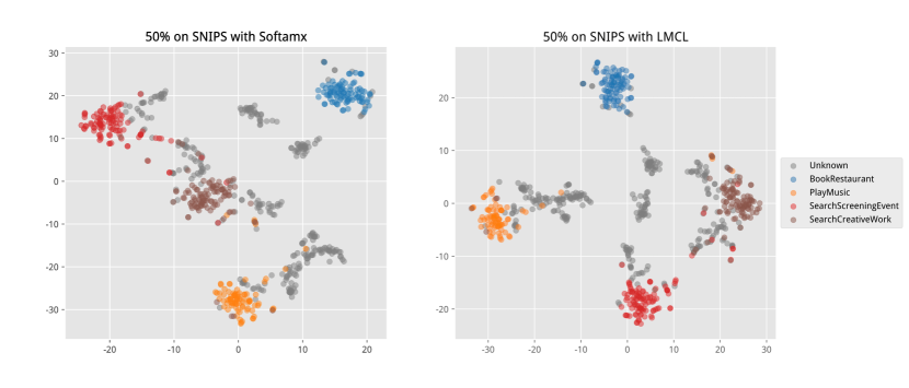
Figure 2: Visualization of deep features learned with softmax and LMCL on SNIPS dataset.

3 Experiments

3.1 Datasets

We have conducted experiments on two publicly available benchmark dialogue datasets, including SNIPS and ATIS Tür et al. (2010). The detailed statistics are shown in Table 1.

SNIPS SNIPS is a personal voice assistant dataset which contains 7 types of user intents across different domains.

ATIS (Airline Travel Information System) ATIS dataset contains recordings of people making reservations with 18 types of user intent in the flight domain.

3.2 Baselines

We compare our methods with state-of-the-art methods and a variant of the proposed method.

1. Maximum Softmax Probability (MSP) Hendrycks and Gimpel (2016) Consider the maximum softmax probability of a sample as the score, if a sample does not belong to any known intents, its score will be lower. We calculate and apply a confidence threshold on the score as the simplest baseline where the threshold is set as 0.5.

2. DOC Shu et al. (2017) It is the state-of-the-art method in the field of open-world classification. It replaces softmax with sigmoid activation function as the final layer. It further tightens the decision boundary of the sigmoid function by calculating the confidence threshold for each class through statistics approach.

3. DOC (Softmax) A variant of DOC. It replaces the sigmoid activation function with softmax.

4. LOF (Softmax) A variant of the proposed method for ablation study. We use softmax loss to train the feature extractor rather than LMCL.

3.3 Experimental Settings

We follow the validation setting in Fei and Liu (2016); Shu et al. (2017) by keeping some classes in training as unknown and integrate them back during testing. Then we vary the number of known classes in training set in the range of 25%, 50%, and 75% classes and use all classes for testing.

To conduct a fair evaluation for the imbalanced dataset, we randomly select known classes by weighted random sampling without replacement in the training set. If a class has more examples, it is more likely to be chosen as the known class. Meanwhile, the class with fewer examples still have a chance to be selected. Other classes are regarded as unknown and we will remove them in the training and validation set.

We initialize the embedding layer through GloVe Pennington et al. (2014) pre-trained word vectors . For BiLSTM model, we set the output dimension as 128 and the maximum epoch as 200 with early stop. For LMCL and LOF, we follow the original setting in their paper. We use macro f1-score as the evaluation metric and report the average result over 10 runs. We set the scaling factor $s$ as 30 and cosine margin $m$ as 0.35, which is recommended by Wang et al. (2018a).

3.4 Results and Discussion

We show the experiment results in Table 2. Firstly, our method consistently performs better than all baselines in all settings. Compared with DOC, our method improves the macro f1-score on SNIPS by 6.7%, 16.2% and 14.9% in 25%, 50%, and 75% setting respectively. It confirms the effectiveness of our two-stage approach.

Secondly, our method is also better than LOF (Softmax). In Figure 2, we use t-SNE Maaten and Hinton (2008) to visualize deep features learned with softmax and LMCL. We can see that the deep features learned with LMCL are intra-class compact and inter-class separable, which is beneficial for novelty detection algorithms based on local density.

Thirdly, we observe that on the ATIS dataset, the performance of unknown intent detection dramatically drops as the known intent increases. We think the reason is that the intents of ATIS are all in the same domain and they are very similar in semantics (e.g., flight and flight_no). The semantics of the unknown intents can easily overlap with the known intents, which leads to the poor performance of all methods.

Finally, compared with ATIS, our approach improve even better on SNIPS. Since the intent of SNIPS is originated from different domains, it causes the DNN to learn a simple decision function when the known intents are dissimilar to each other. By replacing the softmax loss with the margin loss, we can push the network to further reduce the intra-class variance and the inter-class variance, thus improving the robustness of the feature extractor.

4 Conclusion

In this paper, we proposed a two-stage method for unknown intent detection. Firstly, we train a BiLSTM classifier as the feature extractor. Secondly, we replace softmax loss with margin loss to learn discriminative deep features by forcing the network to maximize inter-class variance and to minimize intra-class variance. Finally, we detect unknown intents through the novelty detection algorithm. We also believe that broader families of anomaly detection algorithms are also applicable to our method.

Extensive experiments conducted on two benchmark datasets show that our method can yield consistent improvements compared with the baseline methods. In future work, we plan to design a solution that can identify the unknown intent from known intents and cluster the unknown intents in an end-to-end fashion.

References

- Bendale and Boult (2016) Abhijit Bendale and Terrance E. Boult. 2016. Towards open set deep networks. 2016 IEEE Conference on Computer Vision and Pattern Recognition (CVPR), pages 1563–1572.
- Breunig et al. (2000) Markus M Breunig, Hans-Peter Kriegel, Raymond T Ng, and Jörg Sander. 2000. Lof: identifying density-based local outliers. In ACM sigmod record, volume 29, pages 93–104.
- (3) Tomas Brychcin and Pavel Král. Unsupervised dialogue act induction using gaussian mixtures. In Proceedings of the 15th Conference of the European Chapter of the Association for Computational Linguistics, EACL 2017, pages 485–490.
- Fei and Liu (2016) Geli Fei and Bing Liu. 2016. Breaking the closed world assumption in text classification. In Proceedings of the 2016 Conference of the North American Chapter of the Association for Computational Linguistics: Human Language Technologies, pages 506–514.
- Goo et al. (2018) Chih-Wen Goo, Guang Gao, Yun-Kai Hsu, Chih-Li Huo, Tsung-Chieh Chen, Keng-Wei Hsu, and Yun-Nung Chen. 2018. Slot-gated modeling for joint slot filling and intent prediction. In Proceedings of the 2018 Conference of the North American Chapter of the Association for Computational Linguistics: Human Language Technologies, Volume 2 (Short Papers), pages 753–757.
- Hendrycks and Gimpel (2016) Dan Hendrycks and Kevin Gimpel. 2016. A baseline for detecting misclassified and out-of-distribution examples in neural networks. arXiv preprint arXiv:1610.02136.
- Kim and Kim (2018) Joo-Kyung Kim and Young-Bum Kim. 2018. Joint learning of domain classification and out-of-domain detection with dynamic class weighting for satisficing false acceptance rates. In Interspeech 2018, 19th Annual Conference of the International Speech Communication Association, Hyderabad, India, 2-6 September 2018, pages 556–560.
- Liu et al. (2017) Weiyang Liu, Yandong Wen, Zhiding Yu, Ming Li, Bhiksha Raj, and Le Song. 2017. Sphereface: Deep hypersphere embedding for face recognition. In 2017 IEEE Conference on Computer Vision and Pattern Recognition, CVPR 2017, Honolulu, HI, USA, July 21-26, 2017, pages 6738–6746.
- Liu et al. (2016) Weiyang Liu, Yandong Wen, Zhiding Yu, and Meng Yang. 2016. Large-margin softmax loss for convolutional neural networks. In Proceedings of the 33nd International Conference on Machine Learning, ICML 2016, New York City, NY, USA, June 19-24, 2016, pages 507–516.
- Maaten and Hinton (2008) Laurens van der Maaten and Geoffrey Hinton. 2008. Visualizing data using t-sne. Journal of machine learning research, 9(Nov):2579–2605.
- Mesnil et al. (2015) Grégoire Mesnil, Yann Dauphin, Kaisheng Yao, Yoshua Bengio, Li Deng, Dilek Hakkani-Tur, Xiaodong He, Larry Heck, Gokhan Tur, Dong Yu, et al. 2015. Using recurrent neural networks for slot filling in spoken language understanding. IEEE/ACM Transactions on Audio, Speech, and Language Processing, 23(3):530–539.
- Nalisnick et al. (2019) Eric Nalisnick, Akihiro Matsukawa, Yee Whye Teh, Dilan Gorur, and Balaji Lakshminarayanan. 2019. Do deep generative models know what they don’t know? In International Conference on Learning Representations.
- Pennington et al. (2014) Jeffrey Pennington, Richard Socher, and Christopher D Manning. 2014. Glove: Global vectors for word representation. In EMNLP, volume 14, pages 1532–1543.
- Ranjan et al. (2017) Rajeev Ranjan, Carlos D. Castillo, and Rama Chellappa. 2017. L2-constrained softmax loss for discriminative face verification. CoRR, abs/1703.09507.
- Scheirer et al. (2013) Walter J. Scheirer, Anderson Rocha, Archana Sapkota, and Terrance E. Boult. 2013. Toward open set recognition. IEEE Transactions on Pattern Analysis and Machine Intelligence, 35:1757–1772.
- Shu et al. (2017) Lei Shu, Hu Xu, and Bing Liu. 2017. Doc: Deep open classification of text documents. In Proceedings of the 2017 Conference on Empirical Methods in Natural Language Processing, EMNLP 2017, Copenhagen, Denmark, September 9-11, 2017, pages 2911–2916.
- Tür et al. (2010) Gökhan Tür, Dilek Z. Hakkani-Tür, and Larry P. Heck. 2010. What is left to be understood in atis? 2010 IEEE Spoken Language Technology Workshop, pages 19–24.
- Wang et al. (2018a) Feng Wang, Jian Cheng, Weiyang Liu, and Haijun Liu. 2018a. Additive margin softmax for face verification. IEEE Signal Processing Letters, 25(7):926–930.
- Wang et al. (2018b) Hao Wang, Yitong Wang, Zheng Zhou, Xing Ji, Dihong Gong, Jingchao Zhou, Zhifeng Li, and Wei Liu. 2018b. Cosface: Large margin cosine loss for deep face recognition. In 2018 IEEE Conference on Computer Vision and Pattern Recognition, CVPR 2018, Salt Lake City, UT, USA, June 18-22, 2018, pages 5265–5274.
- Wang et al. (2018c) Yu Wang, Yilin Shen, and Hongxia Jin. 2018c. A bi-model based rnn semantic frame parsing model for intent detection and slot filling. In Proceedings of the 2018 Conference of the North American Chapter of the Association for Computational Linguistics: Human Language Technologies, NAACL-HLT 2018, pages 309–314.
- Yu et al. (2017) Yang Yu, Wei-Yang Qu, Nan Li, and Zimin Guo. 2017. Open-category classification by adversarial sample generation. In Proceedings of the Twenty-Sixth International Joint Conference on Artificial Intelligence, IJCAI 2017, pages 3357–3363.