Finite size effects in the free energy density for Abelian (anti-)self-dual gluon field in $SU(3)$ gluodynamics

Abstract

Finite-size effects in the free energy density for Abelian (anti-)self-dual gluon field are investigated within $SU(3)$ gluodynamics. In particular, the role of gluon quasi-zero modes is studied. The effective potential is calculated within the framework of zeta function regularization for finite spherical four-dimensional region of radius $R$ in Euclidean space-time. In order to obtain the correct strong-field behavior of the effective potential which is determined by the asymptotic freedom, the quasi-zero gluon modes have to be treated beyond one-loop approximation in line with the argumentaion of Leutwyler Leutwyler (1981). Conditions for appearance of the global minimum of the free energy density at finite nonzero values of both field strength and region size are discussed.

I Introduction

There exists certain evidence that physical QCD vacuum can be rather efficiently represented by the statistical ensemble of almost everywhere homogeneous Abelian (anti-)self-dual gluon field configurations. Indications come from study of QCD effective action by various methods Minkowski (1978); Leutwyler (1980, 1981); Pagels and Tomboulis (1978); Trottier and Woloshyn (1993); Galilo and Nedelko (2011); Eichhorn et al. (2011) and application of the model of confinement, chiral symmetry breaking and hadronization in QCD, which is based on this representation of QCD vacuum, to calculation of hadron spectra, decay constants and formfactors Efimov and Nedelko (1995); Kalloniatis and Nedelko (2001, 2004); Nedelko and Voronin (2016, 2017). In particular, study of the effective action demonstrated that homogeneous Abelian (anti-)self-dual field appears to be a good candidate for a global minimum of the effective action Leutwyler (1981); Eichhorn et al. (2011), and that there exist kink-like defects in the Abelian (anti-)self-dual homogeneous gluon background field Galilo and Nedelko (2011) allowing one to explicitly represent general almost everywhere homogeneous Abelian (anti-)self-dual field configurations in the form of domain wall networks Nedelko and Voronin (2015). Above-mentioned hadronization model implies not only the domain wall networks themselves, but also the existence of mean finite size of the regions with homogeneous field (domain bulk) in the typical domain wall network. This in turn requires certain mechanism that prevents domain size from infinite growth. One potentially possible mechanism involves lower-dimentional topologically stable vortex, monopole and instanton-like configurations at the domain wall junctions which may stabilize the domain size. Another mechanism may relate to the non-monotonic dependence of the domain energy on its size, such that the energy minimum corresponds to certain finite size. In fact, these scenarios may complement each other.

In the present paper we investigate the second mechanism for pure gluodynamics, and observe that gluon quasi-zero modes can be crucially important for domain size stabilization. Namely, the free energy density (effective potential density) of the four-dimensional spherical domain with radius $R$ filled by the (anti-)self-dual Abelian field is calculated to the lowest non-vanishing order in gluon and ghost field fluctuations. The case of full QCD with quarks will be considered elsewhere.

The free energy density $F$ is defined by the Euclidean functional integral

$$\exp\left(-V_{R}F(B,R)\right)=N\int_{\mathscr{Q}}\mathscr{D}Q\int_{\mathscr{C}}\mathscr{D}C\mathscr{D}C^{\dagger}\exp\left\{-\int_{V_{R}}d^{4}x\ \mathscr{L}(Q,C^{\dagger},C,B)\right\},$$ (1)

where $V_{R}$ is the volume of four-dimensional spherical region with radius $R$, and $\mathscr{L}(Q,C^{\dagger},C,B)$ is the standard gauge-fixed Yang–Mills Lagrangian in the background gauge in the presence of the background gluon field

$$\breve{B}_{\mu}=\breve{n}B_{\mu},\quad\breve{n}=T_{3}\cos\xi+T_{8}\sin\xi,\quad B_{\mu}=-\frac{1}{2}B_{\mu\nu}x_{\nu},$$

$$B_{\mu\nu}=\pm\frac{1}{2}\varepsilon_{\mu\nu\alpha\beta}B_{\alpha\beta},\quad B_{\mu\alpha}B_{\nu\alpha}=B^{2}\delta_{\mu\nu},$$

where $\breve{B}_{\mu}$ stands for self-dual or anti-self-dual Abelian gluon field in adjoint representation of $su(3)$, upper sign corresponds to self-dual field, and lower to anti-self-dual field. For finite Euclidean space-time region, the functional spaces $\mathscr{Q}$ and $\mathscr{C}$ contain gauge $Q$ and ghost $C$ fields subject to Dirichlet boundary conditions

$$\left.\breve{n}Q_{\mu}(x)\right|_{x\in\partial V_{R}}=0,\quad\left.\breve{n}C(x)\right|_{x\in\partial V_{R}}=0,$$ (2)

$V_{R}$ is the four-dimensional spherical region with boundary $\partial V_{R}$. Justification of this choice for the boundary conditions can be found in Nedelko and Voronin (2015); Kalloniatis and Nedelko (2001). The normalization $N$ is chosen in such a way that the effective potential is equal to zero at vanishing background field strength.

The functional integral can be defined through decomposition of the gauge and ghost fields,

$$Q(x)=\sum_{n}q_{n}Q^{(n)}(x),\quad C(x)=\sum_{n}c_{n}C_{n}(x),$$

over the basis in $\mathscr{Q}$ and $\mathscr{C}$ given by the eigenfunctions of the corresponding differential operators,

$$\left[-\breve{D}^{2}\delta_{\mu\nu}+2i\breve{B}_{\mu\nu}\right]Q^{(n)}_{\nu}= \lambda_{n}Q^{(n)}_{\mu}$$

$$-\breve{D}^{2}C_{n}= \lambda_{n}C_{n},$$ (3)

subject to boundary condition (2). Indices $n$ above are condensed ones: they include all relevant quantum numbers as described below. It has to be stressed that the spectrum $(\lambda_{n})$ is purely discrete for any $R$ and any finite $B$. Integral (1) takes the form

$$\exp\left(-V_{R}F(B,R)\right)=N\prod_{n,m,k}\int_{\mathscr{Q}}dq_{n}\int_{\mathscr{C}}dc_{m}dc_{k}^{\dagger}\exp\left\{-S(q,c,c^{\dagger},B,R)\right\}.$$ (4)

At finite $R$, all eigenvalues for gauge and ghost fields are positive, and the lowest (one-loop) order result for the free energy is obtained simply through determinants of the differential operators (3). However, there will be neither regular strong-field nor infinite-volume limits for thus obtained free energy due to emergence of gluon zero modes (eigenmodes with zero eigenvalues) in these cases.

Just ommiting the quasi-zero mode part of gauge field is not possible: if contribution of quasi-zero modes is neglected, the strong-field asymptotics of the free energy density does not comply with asymptotic freedom Leutwyler (1981).

As it has been noticed by Leutwyler, contribution of the normal (nonzero) gluon and ghost modes in the functional integral leads to a natural regularization of the zero modes. Already the lowest correction due to normal modes generate a kind of “effective mass” term for zero modes and provides an appropriate Gaussian measure for integration over the zero modes in the functional integral (4). Even though for finite-size region ($R<\infty$) zero modes turn into quasi-zero modes, the separate treatment of normal and quasi-zero modes is necessary. In the case of both strong-field and infinite-size limits, quasi-zero modes correctly tend to the corresponding zero modes. In order to provide the correct infinite-volume and strong-field limits of the effective potential, one has to treat quasi-zero modes beyond one-loop approximation.

In general, the effective “mass” for quasi-zero mode is expected to depend on $R$. In this paper we analyze plausible forms of this behavior and its influence on the free energy density. Straightforward evaluation of this dependence will be given elsewhere. It is shown that incorporation of constant effective mass derived by Leutwyler for infinite volume leads to global minimum of the free energy density at nonzero finite $B$ and $R\to\infty$. This means that domain size would grow infinitely in pure gluodynamics. For effective “mass” vanishing at $R\to 0$, which is expected due to the rapid growth of all eigenvalues at small $R$, a global minimum at finite $B$ and $R$ arises. Thus our main observation is that gluon quasi-zero modes may be crucially important for domain size stabilization.

The paper is organized as follows. Calculation of the free energy density is given in Section II. Various scenarios for dependence of zero mode “mass” on domain size are analyzed in Section III. The procedure of calculation of zeta-regularized determinants for ghost and gauge fields is described in detail in Appendix A. Auxiliary formulas are summarized in Appendices B and C. It should be noted that the calculational technique is one of the results by itself and is inseparable from the general physical content of the paper.

II Free energy density

Classical part of free energy density is given by

$$F^{\textrm{cl}}=B^{2}/g^{2}.$$

According to (4), one-loop contribution to the free energy is given by

$$\delta U=V_{R}\delta F(B,R)=\frac{1}{2}\mathrm{Tr}\ln\Delta^{\mathrm{gl}}-\mathrm{Tr}\ln\Delta^{\mathrm{gh}}.$$ (5)

Here $\Delta^{\mathrm{gl}}$ and $\Delta^{\mathrm{gh}}$ stand for corresponding operators in (3). We use analytical regularization

$$\mathrm{Tr}\log\Delta=-\frac{d}{ds}\sum_{j}\left.\lambda_{j}^{-s}\vphantom{\frac{1}{1}}\right|_{s=0}=-\left.\frac{d}{ds}\zeta(s)\right|_{s=0},$$

where $\lambda$ are eigenvalues of operator $\Delta$. The method of computation of $\zeta(s)$ employed in the present study is summarized in Refs. Bordag et al. (1996); Kirsten (2001).

The most straightforward calculation relates to the ghost fields. Operator $\Delta$ in this case is simply

$$\Delta^{\mathrm{gh}}=-\breve{D}^{2},\quad\breve{D}_{\mu}=\partial_{\mu}-i\breve{B}_{\mu},$$

where $\breve{B}_{\mu}$ stands for self-dual or anti-self-dual Abelian gluon field in adjoint representation of $su(3)$. The eigenvalues $\lambda$ of operator $\breve{D}^{2}$ are defined by equation Kalloniatis and Nedelko (2001)

$$M\left(\frac{k}{2}+1-m-\frac{\lambda^{2}}{2n_{a}B},k+2,\frac{n_{a}BR^{2}}{2}\right)=0,\ k=0,1,2,\dots,\ m=-\frac{k}{2},-\frac{k}{2}+1,\dots,\frac{k}{2}.$$

Here $n_{a}$ is the $a$-th nonzero eigenvalue of $\breve{n}$. The eigenmodes corresponding to zero eigenvalues of $\breve{n}$ do not depend on $B$ and hence do not contribute to the effective potential. Every solution of this equation with given $k,m$, radial number $r$ and $a$ is $k+1$-degenerate. The spectrum is invariant with respect to $B\to-B$ which is evident if one performs Kummer transformation. In the limit $B\to 0$ equation for eigenvalues transforms to (see Appendix B)

$$(k+1)!\left(\frac{\lambda R}{2}\right)^{-k-1}J_{k+1}(\lambda R)=0.$$

The normalized one-loop contribution to effective potential is defined as

$$\delta U^{\mathrm{gh}}=-\mathrm{Tr}\ln\frac{-\breve{D}^{2}}{-\breve{\partial}^{2}}=-\sum_{kmr}\mathrm{Tr}_{\mathrm{c}}\ln\frac{\lambda_{kmr}^{2}(\breve{B},R)}{\lambda_{kmr}^{2}(0,R)}=\left.\frac{d}{ds}\zeta^{\mathrm{gh}}(s)\right|_{s=0},$$

where $\mathrm{Tr}_{\mathrm{c}}$ is trace with respect to color indices, and dimensionless quantities

$$\lambda\to\lambda/\mu,\quad B\to B/\mu^{2},\quad R\to R\mu$$

are introduced, $\mu$ is an arbitrary scale.

Following Refs. Bordag et al. (1996); Kirsten (2001), we can define zeta function as

$$\zeta^{\text{gh}}(s)=\mathrm{Tr}_{\mathrm{c}}\frac{\sin\pi s}{\pi}\sum_{k=0}^{\infty}\sum_{m=-\frac{k}{2}}^{\frac{k}{2}}(k+1)\int_{0}^{\infty}\frac{dt}{t^{2s}}\frac{d}{dt}\Psi^{\mathrm{gh}}(k+1,m,t,\breve{B},R),$$

$$\Psi^{\mathrm{gh}}(k,m,t,\breve{B},R)=\log\frac{\exp\left(-\frac{\breve{B}R^{2}}{4}\right)M\left(\frac{k+1}{2}-m+\frac{t^{2}}{2\breve{B}},k+1,\frac{\breve{B}R^{2}}{2}\right)}{k!\left(\frac{tR}{2}\right)^{-k}I_{k}(tR)}.$$

This expression is still formal and divergent because regions of convergence of the integral and sums do not overlap. To make it finite at $s\to 0$, several terms of asymptotic decompositon of integrand in $k\gg 1$ are added and subtracted

$$\zeta^{\text{gh}}(s)=\mathrm{Tr}_{\mathrm{c}}\left\{\frac{\sin\pi s}{\pi}\sum_{k=1}^{\infty}k^{1-2s}\int_{0}^{\infty}\frac{dt}{t^{2s}}\frac{d}{dt}\left[\sum_{m=-\frac{k-1}{2}}^{\frac{k-1}{2}}\Psi^{\mathrm{gh}}(k,m,kt,\breve{B},R)-\sum_{i=0}^{2}\frac{u_{i}^{\mathrm{gh}}(t,\breve{B},R)}{k^{i}}\right]\right.\\ \left.+\frac{\sin\pi s}{\pi}\sum_{k=1}^{\infty}k^{1-2s}\int_{0}^{\infty}\frac{dt}{t^{2s}}\frac{d}{dt}\sum_{i=0}^{2}\frac{u_{i}^{\mathrm{gh}}(t,\breve{B},R)}{k^{i}}\right\}$$ (6)

The first term in the curly brackets is analytical at $s\to 0$. The sums and integrals in the second term are expressed via analytical functions in the regions of $s$ where they converge, and analytically continued to $s\to 0$ in the complex plane (see Appendix A for details). The final expression for $\delta U^{\mathrm{gh}}$ is

$$\delta U^{\mathrm{gh}}(B,R)=-4\sum_{k=1}^{\infty}k\left[\sum_{m=-\frac{k-1}{2}}^{\frac{k-1}{2}}\Psi^{\text{gh}}(k,m,0,\frac{\sqrt{3}B}{2},R)-\frac{3}{4}B^{2}R^{4}\frac{1}{48}\left(1-\frac{1}{k}+\frac{1}{k^{2}}\right)\right]\\ +\frac{B^{2}R^{4}}{48}(2-3\gamma+3\log 2-3\log R)-\frac{3B^{4}R^{8}}{10240}.$$ (7)

The first term is convergent sum that is computed numerically. The contribution of ghosts to one-loop free energy density given by Eq. (7) is shown in Fig. 1.

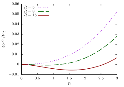
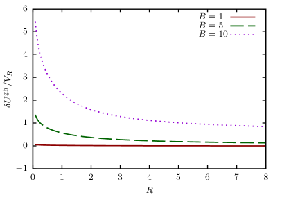
Figure 1: Figures of free energy density of ghost field $\delta F^{\textrm{gh}}(B,R)=\delta U^{\text{gh}}/V_{R}$ at different values of $R$ and $B$. There is a minimum versus $B$ if $R$ is sufficiently large. At large $R$, $\delta F^{\textrm{gh}}(B,R)$ tends to a constant.

Completely analogous considerations for gluon field in Feynman gauge with

$$\Delta_{\mu\nu}^{\mathrm{gl}}=-\breve{D}^{2}\delta_{\mu\nu}+2iB_{\mu\nu}$$

lead to equation

$$\delta U^{\mathrm{gl}}(B,R)=4\sum_{k=1}^{\infty}k\left[\sum_{m=-\frac{k-1}{2}}^{\frac{k-1}{2}}\Psi^{\text{gl}}(k,m,0,\frac{\sqrt{3}B}{2},R)-\frac{3}{4}B^{2}R^{4}\frac{1}{24}\left(1-\frac{1}{k}-\frac{5}{k^{2}}\right)\right]\\ -\frac{B^{2}R^{4}}{48}(31+30\gamma-30\log 2+30\log R)+\frac{3B^{4}R^{8}}{5120}.$$ (8)

Contribution of $SU(3)$ gluodynamics to the effective potential of Abelian (anti-)self-dual gluon fields in finite volume is given by sum of Eqs. (7) and (8).

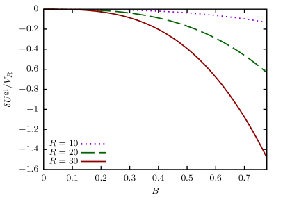
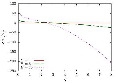
Figure 2: Figures of free energy density of gluon field $\delta F^{\textrm{gl}}(B,R)=\delta U^{\text{gl}}/V_{R}$ (only one-loop contribution) at different values of $R$ and $B$. The strong-field asymptotics is incorrect, and there is no minimum with respect to $B$. $\delta F^{\textrm{gl}}(B,R)$ does not have large-size limit.

Free energy density of gluons $\delta F^{\textrm{gl}}(B,R)$ is shown in Fig. 2. It is easily seen that behavior at large $B$ and $R$ does not comply with predictions of renormalization group Savvidy (1977); Matinyan and Savvidy (1978) and results of calculations in infinite volume Leutwyler (1981). Free energy density decreases at large $B$ and fixed $R$, and $\delta F^{\textrm{gl}}(B,R)$ does not approach a constant value at large $R$ and fixed $B$. This problem is a manifestation of quasi-zero gauge field eigenvalues that tend to zero as $BR^{2}\to\infty$.

If all eigenvalues are sufficiently large to provide Gaussian damping in the functional integral, then perturbation theory is applicable, and formula (5) is justified. The smaller the eigenvalues, the worse the one-loop approximation for contribution of quasi-zero modes. In the limit $BR^{2}\to\infty$ the lowest-order nonvanishing contribution due to quasi-zero modes comes not from the one-loop but from higher orders Leutwyler (1981). Thus, we have to take into account higher order corrections in order to make one-loop effective potential reasonable at large $BR^{2}$. Calculations in the infinite volume is a guiding example. It was shown Leutwyler (1981) that nonzero modes generate an effective “mass term” $\varkappa$ for zero modes. In terms of the present calculation, this mechanism leads to a shift in the quasi-zero eigenvalues $\lambda^{2}$ by a “mass term”

$$\lambda_{\mathrm{eff}}^{2}=\lambda^{2}+\varkappa B,$$

where $\varkappa$ is $B$-independent constant in the case of infinite volume, but in finite region it depends on dimensionless variable $BR^{2}$. Calculation of $\varkappa$ in finite volume is rather complicated, but it is quite easy to estimate the potential effect which the quasi-zero mode “mass” may produce. If for present study we use constant $\varkappa$ that emerges in the case of infinite volume calculation, then incorporation of $\varkappa$ generates a term that restores behavior at large $BR^{2}$ (see Appendix A for details):

$$\delta U_{\varkappa}^{\mathrm{gl}}(B,R)=4\sum_{k=1}^{\infty}k\left[\sum_{m=-\frac{k-1}{2}}^{\frac{k-1}{2}}\Psi^{\text{gl}}(k,m,0,\frac{\sqrt{3}B}{2},R)-\frac{3}{4}B^{2}R^{4}\frac{1}{24}\left(1-\frac{1}{k}-\frac{5}{k^{2}}\right)\right]\\ -\frac{B^{2}R^{4}}{48}(31+30\gamma-30\log 2+30\log R)+\frac{3B^{4}R^{8}}{5120}\\ +4\sum_{k=0}^{\infty}\left[(k+1)\log\frac{\lambda_{k\frac{k}{2}0}^{2}(B,R)+\varkappa B}{\lambda_{k\frac{k}{2}0}^{2}(B,R)}+(k+1)\log\frac{\lambda_{k\frac{-k}{2}0}^{2}(B,R)-\varkappa B}{\lambda_{k\frac{-k}{2}0}^{2}(B,R)}\right].$$ (9)

Corresponding free energy density $\delta F_{\varkappa}^{\textrm{gl}}(B,R)=\delta U_{\varkappa}^{\text{gh}}/V_{R}$ is shown in Fig. 3.

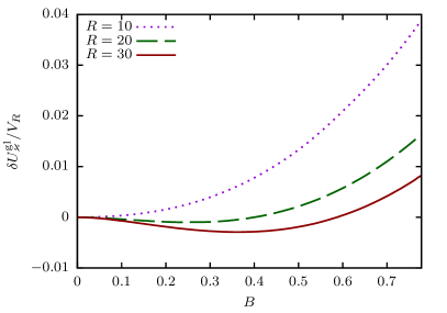
Figure 3: Figures of free energy density $\delta F_{\varkappa}^{\textrm{gh}}(B,R)$ given by (9) at different values of $R$ and $B$ with $\varkappa=1$ incorporated. The correct strong-field asymptotics as well as large-size limit are restored, there is a minimum versus $B$ if $R$ is sufficiently large.

Combining one-loop contributions of gluons and ghosts together, one finds result of straightforward calculation (just calculation of the determinants including quasi-zero modes)

$$\delta U(B,R)=\delta U^{\mathrm{gl}}(B,R)+\delta U^{\mathrm{gh}}(B,R)=4\sum_{k=1}^{\infty}k\left[\sum_{m=-\frac{k-1}{2}}^{\frac{k-1}{2}}\Psi^{\text{gl}}(k,m,0,\frac{\sqrt{3}B}{2},R)-\frac{3}{4}B^{2}R^{4}\frac{1}{24}\left(1-\frac{1}{k}-\frac{5}{k^{2}}\right)\right]\\ -4\sum_{k=1}^{\infty}k\left[\sum_{m=-\frac{k-1}{2}}^{\frac{k-1}{2}}\Psi^{\text{gh}}(k,m,0,\frac{\sqrt{3}B}{2},R)-\frac{3}{4}B^{2}R^{4}\frac{1}{48}\left(1-\frac{1}{k}+\frac{1}{k^{2}}\right)\right]\\ -\frac{B^{2}R^{4}}{48}(29+33\gamma-33\log 2+33\log R)+\frac{3B^{4}R^{8}}{10120}.$$

Taking into account the higher-order “mass term” $\varkappa$ for quasi-zero modes leads to

$$\delta U_{\varkappa}(B,R)=\delta U_{\varkappa}^{\mathrm{gl}}(B,R)+\delta U^{\mathrm{gh}}(B,R)=4\sum_{k=1}^{\infty}k\left[\sum_{m=-\frac{k-1}{2}}^{\frac{k-1}{2}}\Psi^{\text{gl}}(k,m,0,\frac{\sqrt{3}B}{2},R)-\frac{3}{4}B^{2}R^{4}\frac{1}{24}\left(1-\frac{1}{k}-\frac{5}{k^{2}}\right)\right]\\ +4\sum_{k=0}^{\infty}\left[(k+1)\log\frac{\lambda_{\mathrm{gl},k\frac{k}{2}0}^{2}(B,R)+\varkappa B}{\lambda_{\mathrm{gl},k\frac{k}{2}0}^{2}(B,R)}+(k+1)\log\frac{\lambda_{\mathrm{gl},k\frac{-k}{2}0}^{2}(B,R)-\varkappa B}{\lambda_{\mathrm{gl},k\frac{-k}{2}0}^{2}(B,R)}\right]\\ -4\sum_{k=1}^{\infty}k\left[\sum_{m=-\frac{k-1}{2}}^{\frac{k-1}{2}}\Psi^{\text{gh}}(k,m,0,\frac{\sqrt{3}B}{2},R)-\frac{3}{4}B^{2}R^{4}\frac{1}{48}\left(1-\frac{1}{k}+\frac{1}{k^{2}}\right)\right]\\ -\frac{B^{2}R^{4}}{48}(29+33\gamma-33\log 2+33\log R)+\frac{3B^{4}R^{8}}{10120}.$$ (10)

Total free energy density $F=\delta U_{\varkappa}(B,R)/V_{R}$ is shown in Fig. 4. The right-hand side plot indicates that infinite volume limit is well-defined as the free energy approaches constant value for any value of the field strength $B$. The left-hand side plot shows that there exists a minimum in $B$, and the field strength at the minimum decreases with decreasing $R$. In the limit $R\to\infty$, free energy density at strong field $B$ correctly approaches the known one-loop strong-field limit.

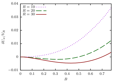
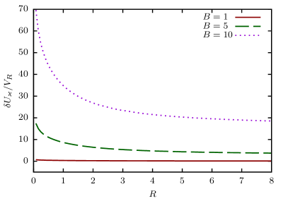
Figure 4: Free energy density $\delta F_{\varkappa}(B,R)$ given by Eq. (10) with $\varkappa=1$.

The total free energy is independent of scale $\mu$ Wiesendanger and Wipf (1994); Cognola et al. (1993):

$$\mu\frac{d}{d\mu}U=0.$$

Combining $\delta U$ (only terms containing $\log R$ contribute to the above equation) with classical term, one obtains

$$\mu\frac{d}{d\mu}\left[\frac{\pi^{2}B^{2}R^{4}}{2g^{2}}-\frac{11}{16}B^{2}R^{4}\log R\right]=0,$$

$$\mu\frac{d}{d\mu}g=-\frac{11g^{3}}{16\pi^{2}}.$$

That is, one-loop $\beta$-function of pure $SU(3)$ gluodynamics is recovered with the choice of boundary conditions adopted in the present study.

III Zero mode “mass” and domain size

As it is shown above, a “mass” $\varkappa$ for quasi-zero modes is required to reproduce correct strong-field asymptotics of the free energy density in the infinite volume limit. However, in the finite volume $\varkappa$ should depend on the size of the domain via dimensionless parameter $z=BR^{2}$. In the previous section calculations were performed with constant value $\varkappa$ in agreement with the infinite volume result. At small $R$ and $B$, eigenvalues for all gluon and ghost modes (including quasi-zero modes) quickly increase Dependence of gluon eigenvalues on $BR^{2}$ is illustrated by Fig. 6. Given that effective “mass” accumulates contributions proportional to the inverse eigenvalues, one may expect that the effective “mass” vanishes at small $z$. Therefore, it is plausible that the effective “mass” satisfies conditions

$$\varkappa(z)\xrightarrow{z\to 0}0,\quad\varkappa(z)\xrightarrow{z\to\infty}\varkappa\not=0.$$

Depending on the profile of the function $\varkappa(z)$, there may exist global minimum of the free energy density with respect to both background field strength $B$ and domain size $R$, which would stabilize the mean size of domains in the ensemble of almost everywhere homogeneous Abelian (anti-)self-dual fields. Free energy density $\delta F_{\varkappa}(B,R)$ with a global minimum in $R$ and $B$ calculated for sample $\varkappa(z)$,

$$\varkappa(z)=\frac{2}{\pi}\left[\arctan\exp\left(\frac{z_{0}-z}{a}\right)+\arctan\exp\left(\frac{z-z_{0}}{a}\right)-2\arctan\exp\left(-\frac{z_{0}}{a}\right)\right],$$ (11)

is shown in Fig.6.

Figure 5: Dependence of solutions of Eq. (13) on $BR^{2}$.

Figure 6: Free energy density $\delta F_{\varkappa}(B,R)$ given by Eq. (10) with $\varkappa$ given by Eq. (11) ($z_{0}=100,a=10$).

To summarize, it becomes clear that explicit calculation of the finite-size dependence of effective quasi-zero “mass” is an important task to be done. Another interesting and important task relates to incorporation of the quark contribution to the free energy density. Quark field in the presence of self-dual gauge field also has (quasi-)zero modes, and their interplay with gluon modes seems to be important for studying the finite size effects in free energy density.

IV Acknowledgements

We acknowledge fruitful discussions with M. Bordag and I.G. Pirozhenko.

Appendix A Zeta function for ghost and gluon fields

A.1 Ghosts

Here we describe calculation of zeta functions in more detail. We start with the expression for $\zeta^{\text{gh}}(s)$ given by (6). Using formula (18) to re-expand $\Psi^{\mathrm{gh}}$ in powers of $k^{-1}$ and summing over $m$, one arrives at the following expressions for $u_{i}^{\mathrm{gh}}$:

$$u_{0}^{\mathrm{gh}}(t,B,R)=B^{2}R^{4}\frac{R^{4}t^{4}-2R^{2}t^{2}-4+4\left(1+R^{2}t^{2}\right)^{1/2}}{24R^{4}t^{4}\left(1+R^{2}t^{2}\right)^{1/2}},$$

$$u_{1}^{\mathrm{gh}}(t,B,R)=-B^{2}R^{4}\frac{1+3R^{2}t^{2}}{48\left(1+R^{2}t^{2}\right)},$$

$$\begin{split}&u_{2}^{\mathrm{gh}}(t,B,R)=\frac{B^{2}R^{4}}{192\left(1+R^{2}t^{2}\right)^{1/2}}\left[\frac{16}{R^{2}t^{2}}+\frac{R^{2}t^{2}(32+7R^{2}t^{2})}{(1+R^{2}t^{2})^{3}}+32\frac{1-\left(1+R^{2}t^{2}\right)^{1/2}}{R^{4}t^{4}}\right]\\ &+\frac{B^{4}R^{8}}{1920\left(1+R^{2}t^{2}\right)^{1/2}}\left[\frac{32}{R^{4}t^{4}}-\frac{128}{R^{6}t^{6}}-\frac{16}{R^{2}t^{2}}+\frac{10+13R^{2}t^{2}}{(1+R^{2}t^{2})^{2}}-256\frac{1-\left(1+R^{2}t^{2}\right)^{1/2}}{R^{8}t^{8}}\right].\end{split}$$

The sums over $k$ are calculated for $\mathfrak{R}s>1$ and analytically continued in terms of Riemann $\zeta$ function

$$\sum_{k=1}^{\infty}\frac{k^{1-2s}}{k^{i}}=\zeta(i-1+2s)$$

to the strip $0<\mathfrak{R}s<1$ where integrals over $t$ converge at $t\to 0$. One obtains

$$\sum_{k=1}^{\infty}k^{1-2s}\int_{0}^{\infty}\frac{dt}{t^{2s}}\frac{d}{dt}\sum_{i=0}^{2}\frac{u_{i}^{\mathrm{gh}}(t,B,R)}{k^{i}}=B^{2}R^{4+2s}\left\{\vphantom{\frac{1}{1}}\right.\zeta(-1+2s)\frac{-\Gamma(2-s)\Gamma(1/2+s)}{24\sqrt{\pi}(2+s)}+\\ \left.\zeta(2s)\frac{\pi s(1-2s)}{48\sin\pi s}+\zeta(1+2s)\frac{\left(6-s(2+s)(11+5s)\right)\Gamma(1-s)\Gamma(3/2+s)}{72\sqrt{\pi}(2+s)}\right\}-B^{4}R^{8+2s}\zeta(1+2s)\frac{s\Gamma(2-s)\Gamma(3/2+s)}{480\sqrt{\pi}(4+s)}.$$

The expansion of counterterms in powers of $s$ around $s=0$ is

$$\frac{\sin\pi s}{\pi}\sum_{k=1}^{\infty}k^{1-2s}\int_{0}^{\infty}\frac{dt}{t^{2s}}\frac{d}{dt}\sum_{i=0}^{2}\frac{u_{i}^{\mathrm{gh}}(t,B,R)}{k^{i}}=\\ B^{2}R^{4}\left[-\frac{1}{96}+\frac{1}{288}(4-6\gamma+\log 64-6\log R)s\right]+B^{4}R^{8}\left[-\frac{1}{7680}s\right]+O(s^{2}),$$

where $\gamma=0.5772156649\dots$ is Euler’s constant, and

$$\mathrm{Tr}\breve{n}^{2}=3,\quad\mathrm{Tr}\breve{n}^{4}=4\frac{9}{16}=\frac{9}{4}.$$

Since the whole spectrum is invariant with respect to $B\to-B$, trace over color leads to factor 4. Evaluating the derivative of $\zeta^{\mathrm{gh}}(s)$ with respect to $s$ at $s=0$, one arrives at the expression (7).

A.2 Gluons

The same procedure is applied to zeta function of gluons. With Dirichlet boundary condition for color-charged modes, the whole set of eigenvalues is determined by the equations Kalloniatis and Nedelko (2001)

$$M\left(\frac{k}{2}+1-m\pm 1-\frac{\lambda^{2}}{2n_{a}B},k+2,\frac{n_{a}BR^{2}}{2}\right)=0,\quad k=0,1,\dots\quad m=-\frac{k}{2},\dots,\frac{k}{2},$$

and every solution of these equations with given $k,m$ and $a$ is $2(k+1)$-degenerate. Repeating the procedure carried out for ghosts, one finds

$$\zeta^{\text{gl}}(s)=\mathrm{Tr}_{\mathrm{c}}\frac{\sin\pi s}{\pi}\sum_{k=0}^{\infty}\sum_{m=-\frac{k}{2}}^{\frac{k}{2}}2(k+1)\int_{0}^{\infty}\frac{dt}{t^{2s}}\frac{d}{dt}\Psi^{\mathrm{gl}}(k+1,m,t,\breve{B},R)=\\ 2\mathrm{Tr}_{\mathrm{c}}\left\{\frac{\sin\pi s}{\pi}\sum_{k=1}^{\infty}k^{1-2s}\int_{0}^{\infty}\frac{dt}{t^{2s}}\frac{d}{dt}\left[\sum_{m=-\frac{k-1}{2}}^{\frac{k-1}{2}}\Psi^{\mathrm{gl}}(k,m,kt,\breve{B},R)-\sum_{i=0}^{2}\frac{u_{i}^{\mathrm{gl}}(t,\breve{B},R)}{k^{i}}\right]\right.\\ \left.+\frac{\sin\pi s}{\pi}\sum_{k=1}^{\infty}k^{1-2s}\int_{0}^{\infty}\frac{dt}{t^{2s}}\frac{d}{dt}\sum_{i=0}^{2}\frac{u_{i}^{\mathrm{gl}}(t,\breve{B},R)}{k^{i}},\right\}$$ (12)

where

$$\begin{split}\Psi^{\mathrm{gl}}(k,m,t,B,R)=\log\frac{\exp\left(-\frac{BR^{2}}{2}\right)M\left(\frac{k+1}{2}-m+1+\frac{t^{2}}{2B},k+1,\frac{BR^{2}}{2}\right)M\left(\frac{k+1}{2}-m-1+\frac{t^{2}}{2B},k+1,\frac{BR^{2}}{2}\right)}{\left(k!\left(\frac{tR}{2}\right)^{-k}I_{k}(tR)\right)^{2}}.\end{split}$$

Coefficients of asymptotic expansion $u_{i}^{\mathrm{gl}}$ are given by

$$u_{0}^{\mathrm{gl}}(t,B,R)=B^{2}R^{4}\frac{R^{4}t^{4}-2R^{2}t^{2}-4+4\left(1+R^{2}t^{2}\right)^{1/2}}{12R^{4}t^{4}\left(1+R^{2}t^{2}\right)^{1/2}},$$

$$u_{1}^{\mathrm{gl}}(t,B,R)=-B^{2}R^{4}\frac{1+3R^{2}t^{2}}{24\left(1+R^{2}t^{2}\right)},$$

$$\begin{split}&u_{2}^{\mathrm{gl}}(t,B,R)=\frac{B^{2}R^{4}}{96\left(1+R^{2}t^{2}\right)^{1/2}}\left[-\frac{80}{R^{2}t^{2}}+\frac{R^{2}t^{2}(32+7R^{2}t^{2})}{(1+R^{2}t^{2})^{3}}-160\frac{1-\left(1+R^{2}t^{2}\right)^{1/2}}{R^{4}t^{4}}\right]\\ &+\frac{B^{4}R^{8}}{960\left(1+R^{2}t^{2}\right)^{1/2}}\left[-\frac{128}{R^{6}t^{6}}+\frac{32}{R^{4}t^{4}}-\frac{16}{R^{2}t^{2}}+\frac{10+13R^{2}t^{2}}{(1+R^{2}t^{2})^{2}}-256\frac{1-\left(1+R^{2}t^{2}\right)^{1/2}}{R^{8}t^{8}}\right].\end{split}$$

And one obtains the following analytical continuation of the counterterms

$$\sum_{k=1}^{\infty}k^{1-2s}\int_{0}^{\infty}\frac{dt}{t^{2s}}\frac{d}{dt}\sum_{i=0}^{2}\frac{u_{i}^{\mathrm{gl}}(t,B,R)}{k^{i}}=B^{2}R^{4+2s}\left\{\vphantom{\frac{1}{1}}\right.\zeta(-1+2s)\frac{-\Gamma(2-s)\Gamma(1/2+s)}{12\sqrt{\pi}(2+s)}+\zeta(2s)\frac{\pi s(1-2s)}{24\sin\pi s}+\\ \left.\zeta(1+2s)\frac{\left(30+s(2+s)(11+5s)\right)\Gamma(1-s)\Gamma(3/2+s)}{36\sqrt{\pi}(2+s)}\right\}-B^{4}R^{8+2s}\zeta(1+2s)\frac{s\Gamma(2-s)\Gamma(3/2+s)}{240\sqrt{\pi}(4+s)}.$$

Now, counterterms can be expanded in powers of $s$:

$$\frac{\sin\pi s}{\pi}\sum_{k=1}^{\infty}k^{1-2s}\int_{0}^{\infty}\frac{dt}{t^{2s}}\frac{d}{dt}\sum_{i=0}^{2}\frac{u_{i}^{\mathrm{gl}}(t,B,R)}{k^{i}}=\\ B^{2}R^{4}\left[\frac{5}{48}+\frac{1}{144}(31+30\gamma-30\log 2+30\log R)s\right]+B^{4}R^{8}\left[-\frac{1}{3840}s\right]+O(s^{2}).$$

Finally,

$$\delta U^{\mathrm{gl}}(B,R)=-\frac{1}{2}\left.\frac{d}{ds}\zeta^{\text{gl}}(s)\right|_{s=0}=4\sum_{k=1}^{\infty}k\left[\sum_{m=-\frac{k-1}{2}}^{\frac{k-1}{2}}\Psi^{\text{gl}}(k,m,0,\frac{\sqrt{3}B}{2},R)-\frac{3}{4}B^{2}R^{4}\frac{1}{24}\left(1-\frac{1}{k}-\frac{5}{k^{2}}\right)\right]\\ -\frac{B^{2}R^{4}}{48}(31+30\gamma-30\log 2+30\log R)+\frac{3B^{4}R^{8}}{5120}.$$

A.3 Contribution of quasi-zero modes

As it is explained in Section II, simple one-loop expression for $\delta U^{\mathrm{gl}}(B,R)$ has incorrect asymptotic behavior versus $B$ and $R$ due to quasi-zero modes of gluons. Now, let us calculate the contribution of quasi-zero modes $\lambda_{k\frac{k}{2}0}$ to the effective potential. These modes are given by lowest solutions of the equations

$$M\left(-\frac{\lambda^{2}}{2|\breve{B}|},k+2,\frac{|\breve{B}|R^{2}}{2}\right)=0,\quad k=0,1,2,\dots$$ (13)

that reduce to

$$\left(\frac{\lambda R}{2}\right)^{-k-1}J_{k+1}(\lambda R)=0,\quad k=0,1,\dots$$

at $B\to 0$. The contribution of quasi-zero modes to the effective potential can be expressed as

$$\delta U^{\textrm{gl}(0)}(B,R)=\frac{1}{2}\textrm{Tr}\log\frac{\lambda_{k\frac{k}{2}0}^{2}(B,R)}{\lambda_{k0}^{2}(0,R)}=\left.-\frac{1}{2}\frac{d}{ds}\zeta^{\textrm{gl}(0)}(s)\right|_{s=0},$$

$$\zeta^{\textrm{gl}(0)}(s)=2\mathrm{Tr}_{\mathrm{c}}\sum_{k=0}^{\infty}(k+1)\left(\lambda_{k\frac{k}{2}0}^{-2s}(B,R)-\lambda_{k0}^{-2s}(0,R)\right),$$ (14)

where factor $2$ in the definition of $\zeta^{\textrm{gl}(0)}(s)$ originates from two polarizations of quasi-zero gluon modes. For the sake of brevity we omit color eigenvalue and restore it in the final answer ($B\to\frac{\sqrt{3}}{2}B$ for adjoint representation of $su(3)$).

To continue $\zeta(s)$ to $s\to 0$, we add and subtract several terms of asymptotic expansion in $k\gg 1$ of $d\zeta/dB$ and $d^{2}\zeta/dB^{2}$ at $B=0$. $\lambda(B)$ is given implicitly via Eq. (13), and we find derivatives

$$\left.\frac{d\lambda_{k\frac{k}{2}0}(B,R)}{dB}\right|_{B=0}=-\frac{k+2}{2\lambda_{k0}(0,R)},\ \left.\frac{d^{2}\lambda_{k\frac{k}{2}0}(B,R)}{dB^{2}}\right|_{B=0}=-\frac{k^{2}+8k+12-\lambda_{k0}^{2}(0,R)R^{2}}{12\lambda_{k0}^{3}(0,R)},$$

where we used identities (Abramowitz and Stegun (1972), 9.1.27)

$$J_{\nu-1}(z)+J_{\nu+1}=\frac{2\nu}{z}J_{\nu}(z),\quad J^{\prime}_{\nu}(z)=-J_{\nu+1}(z)+\frac{\nu}{z}J_{\nu}(z)$$

and the fact that

$$J_{k+1}(\lambda_{k0}(0,R)R)=0.$$

We obtain

$$\begin{split}\left.\frac{d\zeta^{\textrm{gl}(0)}}{dB}\right|_{B=0}&=8\sum_{k=0}^{\infty}(k+1)(-2s)\lambda_{k\frac{k}{2}0}^{-2s-1}(B,R)\left.\frac{d\lambda_{k\frac{k}{2}0}(B,R)}{dB}\right|_{B=0}\\ &=8\sum_{k=0}^{\infty}(k+1)(-2s)\lambda_{k\frac{k}{2}0}^{-2s-1}(0,R)\left(-\frac{k+2}{2\lambda_{k0}(0,R)}\right)=8\sum_{k=1}^{\infty}\zeta_{k}^{(1)},\end{split}$$ (15)

$$\begin{split}\left.\frac{d^{2}\zeta^{\textrm{gl}(0)}}{dB^{2}}\right|_{B=0}=&8\sum_{k=0}^{\infty}(k+1)\left[(-2s)(-2s-1)\lambda_{k\frac{k}{2}0}^{-2s-2}(0,R)\left(-\frac{k+2}{2\lambda_{k0}(0,R)}\right)^{2}\right.\\ &\left.-2s\lambda_{k\frac{k}{2}0}^{-2s-1}(0,R)\left(-\frac{k^{2}+8k+12-\lambda_{k0}(0,R)R^{2}}{12\lambda_{k0}^{3}(0,R)}\right)\right]=8\sum_{k=1}^{\infty}\zeta_{k}^{(2)},\end{split}$$ (16)

where additional factor $4$ is due to color trace. Note that summation index is shifted $k\to k-1$ in the definition of $\zeta^{(i)}_{k}$. Next, we use uniform asymptotic expansion of zeros of Bessel functions (see DLMF , Eq. 10.21.vii)

$$\rho_{\nu}(t)=\nu\sum_{k=0}^{\infty}\frac{\alpha_{k}}{\nu^{2k/3}},\quad\theta\left(-2^{\frac{1}{3}}\alpha\right)=\pi t,\quad\alpha_{0}=1,\quad\alpha_{1}=\alpha,\dots,$$

where $\theta(x)$ is the phase of Airy functions

$$\theta(x)=\arctan\frac{\mathrm{Ai}(x)}{\mathrm{Bi}(x)}.$$

With $t=1$ this formula gives the desired expansion for the first zero $z\neq 0$ of $J_{\nu}(z)$, where $\alpha=1.855757\dots$ Substituting this expansion into Eqs. (15) and (16) and re-expanding in powers of $k^{-1}$, we find

$$\zeta_{k}^{(1)}=R^{2+2s}s\left[k^{-2s}-2\alpha(1+s)k^{-2/3-2s}+k^{-1-2s}\right]+O\left(k^{-4/3-2s}\right)=Z_{k}^{(1)}+O\left(k^{-4/3-2s}\right),$$

$$\zeta_{k}^{(2)}=R^{4+2s}k^{-1-2s}\frac{s}{2}(1+2s)+O\left(k^{-5/3-2s}\right)=Z_{k}^{(2)}+O\left(k^{-5/3-2s}\right).$$

Next, we split $\zeta^{\textrm{gl}(0)}$ into two parts

$$\zeta^{\textrm{gl}(0)}(s)=8\left\{\sum_{k=0}^{\infty}\left[(k+1)\left(\lambda_{k\frac{k}{2}0}^{-2s}(B,R)-\lambda_{k0}^{-2s}(0,R)\right)-BZ_{k+1}^{(1)}-\frac{B^{2}}{2}Z_{k+1}^{(2)}\right]+B\sum_{k=0}^{\infty}Z_{k+1}^{(1)}+\frac{B^{2}}{2}\sum_{k=0}^{\infty}Z_{k+1}^{(2)}\right\}.$$

The first sum is an analytic function for $\mathfrak{R}s>0$. The remaining sums are evaluated for $\mathfrak{R}s>1/2$ and analytically continued to $s\to 0$:

$$Z^{(1)}=\sum_{k=1}^{\infty}Z_{k}^{(1)}=R^{2+2s}s\left[\zeta(2s)-2\alpha(1+s)\zeta\left(\frac{2}{3}+2s\right)+\zeta(1+2s)\right],$$

$$Z^{(2)}=\sum_{k=1}^{\infty}Z_{k}^{(2)}=R^{4+2s}\frac{s}{2}(1+2s)\zeta(1+2s).$$

Finally, we obtain

$$\delta U^{\textrm{gl}(0)}(B,R)=-\frac{1}{2}\left.\frac{d}{ds}\zeta^{\textrm{gl}(0)}(s)\right|_{s=0}=\\ -4\sum_{k=0}^{\infty}\left[-(k+1)\log\frac{\lambda_{k\frac{k}{2}0}^{2}(B,R)}{\lambda_{k0}^{2}(0,R)}-BR^{2}\left(1-2\alpha(k+1)^{-2/3}+(k+1)^{-1}\right)-\frac{B^{2}R^{4}}{4(k+1)}\right]\\ -2BR^{2}\left[-1+2\gamma+2\log R-4\alpha\zeta\left(\frac{2}{3}\right)\right]-B^{2}R^{4}(1+\gamma+\log R).$$

A.4 Contribution of quasi-zero modes with effective “mass”

If one includes “mass term” $\varkappa$ for quasi-zero modes, the formulas for the effective potential become

$$\delta U_{\varkappa}^{\textrm{gl}(0)}(B,R)=\frac{1}{2}\textrm{Tr}\log\frac{\lambda_{k\frac{k}{2}0}^{2}(B,R)+\varkappa B}{\lambda_{k0}^{2}(0,R)}=\left.-\frac{1}{2}\frac{d}{ds}\zeta^{\textrm{gl}(0)}(s)\right|_{s=0},$$

$$\zeta_{\varkappa}^{\textrm{gl}(0)}(s)=2\mathrm{Tr}_{\mathrm{c}}\sum_{k=0}^{\infty}(k+1)\left(\left(\lambda_{k\frac{k}{2}0}^{2}(B,R)+\varkappa B\right)^{-s}-\lambda_{k0}^{-2s}(0,R)\right).$$ (17)

In complete analogy to contribution without $\varkappa$,

$$\left.\frac{d\zeta_{\varkappa}^{\textrm{gl}(0)}}{dB}\right|_{B=0}=8\sum_{k=1}^{\infty}\zeta_{\varkappa k}^{(1)},\quad\left.\frac{d^{2}\zeta_{\varkappa}^{\textrm{gl}(0)}}{dB^{2}}\right|_{B=0}=8\sum_{k=1}^{\infty}\zeta_{\varkappa k}^{(2)}.$$

The corresponding asymptotic expansions in powers of $k$ are

$$\zeta_{\varkappa k}^{(1)}=R^{2+2s}s\left[k^{-2s}-2\alpha(1+s)k^{-2/3-2s}+\left(1-\varkappa\right)k^{-1-2s}\right]+O\left(k^{-4/3-2s}\right)=Z_{\varkappa k}^{(1)}+O\left(k^{-4/3-2s}\right),$$

$$\zeta_{\varkappa k}^{(2)}=R^{4+2s}k^{-1-2s}\frac{s}{2}\left(1+2s\right)+O\left(k^{-5/3-2s}\right)=Z_{\varkappa k}^{(2)}+O\left(k^{-5/3-2s}\right).$$

Counterterms are summed for $\mathfrak{R}s>1/2$

$$Z_{\varkappa}^{(1)}=\sum_{k=1}^{\infty}Z_{\varkappa k}^{(1)}=R^{2+2s}s\left[\zeta(2s)-2\alpha(1+s)\zeta\left(\frac{2}{3}+2s\right)+\left(1-\varkappa\right)\zeta(1+2s)\right],$$

$$Z_{\varkappa}^{(2)}=\sum_{k=1}^{\infty}Z_{\varkappa k}^{(2)}=R^{4+2s}\frac{s}{2}\left(1+2s\right)\zeta(1+2s).$$

Finally,

$$\delta U_{\varkappa}^{\textrm{gl}(0)}(B,R)=\\ -4\sum_{k=0}^{\infty}\left[-(k+1)\log\frac{\lambda_{k\frac{k}{2}0}^{2}(B,R)+\varkappa B}{\lambda_{k0}^{2}(0,R)}-BR^{2}\left(1-2\alpha(k+1)^{-2/3}+(1-\varkappa)(k+1)^{-1}\right)-\frac{B^{2}R^{4}}{4(k+1)}\right]\\ -2BR^{2}\left[-1+(2\gamma+2\log R)(1-\varkappa)-4\alpha\zeta\left(\frac{2}{3}\right)\right]-B^{2}R^{4}\left[1+(\gamma+\log R)\right]$$

A.5 Contribution of all eigenmodes with effective “mass” for quasi-zero modes

Now we are ready to incorporate $\varkappa$ for quasi-zero modes into one-loop effective potential. The desired zeta function is written as

$$\zeta_{\varkappa}^{\mathrm{gl}}(s)=\zeta^{\mathrm{gl}}(s)-\zeta^{\textrm{gl}(0)}(s)+\zeta_{\varkappa}^{\textrm{gl}(0)}(s),$$

where zeta functions in right-hand side are given by Eqs. (12),(14) and (17). The corresponding effective potential is given by

$$\delta U_{\varkappa}^{\mathrm{gl}}(B,R)=4\sum_{k=1}^{\infty}k\left[\sum_{m=-\frac{k-1}{2}}^{\frac{k-1}{2}}\Psi^{\text{gl}}(k,m,0,\frac{\sqrt{3}B}{2},R)-\frac{3}{4}B^{2}R^{4}\frac{1}{24}\left(1-\frac{1}{k}-\frac{5}{k^{2}}\right)\right]\\ -\frac{B^{2}R^{4}}{48}(31+30\gamma-30\log 2+30\log R)+\frac{3B^{4}R^{8}}{5120}\\ +4\sum_{k=0}^{\infty}\left[(k+1)\log\frac{\lambda_{k\frac{k}{2}0}^{2}(B,R)+\varkappa B}{\lambda_{k\frac{k}{2}0}^{2}(B,R)}-\varkappa BR^{2}(k+1)^{-1}\right]+4\varkappa BR^{2}(\gamma+\log R).$$

Thus obtained free energy is not an even function of $B$. To restore this property, one adds term $\varkappa$ to contribution of modes $\lambda_{k,-\frac{k}{2},0}^{2}(B,R)$, and beta function of $SU(3)$ gluodynamics emerges. After these steps one obtains formula (9) for free energy.

Appendix B Connection between Kummer and Bessel functions

We find the desired limit from definition of Kummer function via series (Abramowitz and Stegun (1972), 13.1.2)

$$\lim_{z\to 0}M\left(a+\frac{b}{z},c,dz\right)=\lim_{z\to 0}\sum_{n=0}^{\infty}\frac{\left(a+\frac{b}{z}\right)_{n}(dz)^{n}}{(c)_{n}n!}=\sum_{n=0}^{\infty}\frac{(bd)^{n}}{(c)_{n}n!}={{}_{0}F_{1}}(c,bd)$$

$(c)_{n}$ is Pochhammer symbol:

$$(c)_{0}=1,\quad(c)_{n}=c(c+1)\cdots(c+n-1).$$

Comparing series expansions of Bessel functions (Abramowitz and Stegun (1972), 9.1.10, 9.6.10) and hypergeomteric function ${}_{0}F_{1}$, we find

$${{}_{0}F_{1}}(a,z)=\sum_{k=0}^{\infty}\frac{z^{k}\Gamma(a)}{k!\Gamma(a+k)}=(a-1)!\left(\sqrt{z}\right)^{1-a}\left(\sqrt{z}\right)^{a-1}\sum_{k=0}^{\infty}\frac{(\sqrt{z})^{2k}}{k!\Gamma(a-1+k+1)}=(a-1)!\left(\sqrt{z}\right)^{1-a}I_{a-1}(2\sqrt{z}),$$

$${{}_{0}F_{1}}(a,-z)=\sum_{k=0}^{\infty}\frac{(-z)^{k}\Gamma(a)}{k!\Gamma(a+k)}=(a-1)!\left(\sqrt{z}\right)^{1-a}\left(\sqrt{z}\right)^{a-1}\sum_{k=0}^{\infty}\frac{(-1)^{k}(\sqrt{z})^{2k}}{k!\Gamma(a-1+k+1)}=(a-1)!\left(\sqrt{z}\right)^{1-a}J_{a-1}(2\sqrt{z})$$

for $z\geqslant 0$.

Appendix C Asymptotic expansion of $M(\frac{m+1}{2}+\mu-\kappa+n+\mu^{2}t^{2},1+2\mu+m,z)$ as $\mu\to\infty$, $\kappa/\mu$ fixed

We use the method described in Olver (1997). The Whittaker function

$$M_{\kappa-n-\mu^{2}t^{2},\mu+\frac{m}{2}}(z)=\exp\left(-\frac{z}{2}\right)z^{\mu+\frac{m}{2}+\frac{1}{2}}M\left(\frac{1}{2}+\mu+\frac{m}{2}-\kappa+n+\mu^{2}t^{2},1+2\mu+m,z\right)$$

satisfies equation

$$\frac{d^{2}M_{\kappa-n-\mu^{2}t^{2},\mu+\frac{m}{2}}}{dz^{2}}=\left(\frac{1}{4}+\frac{n}{z}+\frac{m^{2}-1}{4z^{2}}+2\mu\left(-\frac{\kappa}{2\mu}+\frac{m}{2z^{2}}\right)+4\mu^{2}\left(\frac{t^{2}}{4z}+\frac{1}{4z^{2}}\right)\right)M_{\kappa-n-\mu^{2}t^{2},\mu+\frac{m}{2}},$$

$$f_{0}(z)=\frac{t^{2}}{4z}+\frac{1}{4z^{2}},\quad f_{1}(z)=-\frac{\kappa}{2\mu}+\frac{m}{2z^{2}},\quad f_{2}(z)=\frac{1}{4}+\frac{n}{z}+\frac{m^{2}-1}{4z^{2}}.$$

Formal solution to the above equation is sought in the form

$$M_{\kappa-n-\mu^{2}t^{2},\mu+\frac{m}{2}}=f_{0}^{-\frac{1}{4}}(z)\exp\left(2\mu\xi(z)\right)X(z)\sum_{s=0}^{\infty}\frac{A_{s}(\xi(z))}{(2\mu)^{s}},$$

where

$$A_{0}=1,\quad X(\xi)=\exp\left(\frac{1}{2}\int d\xi\phi\right),\quad\psi(z)=\frac{f_{2}(z)}{f_{0}(z)}-f_{0}^{-\frac{3}{4}}(z)\frac{d^{2}}{dz^{2}}f_{0}^{-\frac{1}{4}}(z).$$

$$\xi(z)=\int dz\sqrt{f_{0}(z)}=\sqrt{1+t^{2}z}+\log\frac{t\sqrt{z}}{\sqrt{1+t^{2}z}+1},\quad\phi(z)=\frac{f_{1}(z)}{f_{0}(z)},$$

$$\int d\xi\phi=\int dz\frac{d\xi}{dz}\phi=\int dz\sqrt{f_{0}(z)}\frac{f_{1}(z)}{f_{0}(z)}=\int\frac{dz}{\sqrt{1+t^{2}z}}\left(-\frac{\kappa}{\mu}+\frac{m}{z}\right)=-\frac{2\kappa}{\mu t^{2}}\sqrt{1+t^{2}z}+2m\log\frac{t\sqrt{z}}{\sqrt{1+t^{2}z}+1}.$$

The leading asymptotics is

$$M\left(\frac{m+1}{2}+\mu-\kappa+n+\mu^{2}t^{2},1+2\mu+m,z\right)=\\ \exp\left(\frac{z}{2}\right)z^{-\mu-\frac{m}{2}-\frac{1}{2}}M_{\kappa-n-\mu^{2}t^{2},\mu+\frac{m}{2}}(z)\sim C\exp\left(\frac{z}{2}\right)z^{-\mu-\frac{m}{2}-\frac{1}{2}}\frac{\sqrt{2z}}{(1+t^{2}z)^{\frac{1}{4}}}\\ \times\exp\left(2\mu\sqrt{1+t^{2}z}+2\mu\log\frac{t\sqrt{z}}{\sqrt{1+t^{2}z}+1}-\frac{\kappa}{\mu t^{2}}\sqrt{1+t^{2}z}+m\log\frac{t\sqrt{z}}{\sqrt{1+t^{2}z}+1}\right).$$

The multiplicative constant $C$ is fixed by the condition $M\left(a,b,0\right)=1$:

$$M\left(\frac{m+1}{2}+\mu-\kappa+n+\mu^{2}t^{2},1+2\mu+m,z\right)\sim\\ \exp\left(\frac{z}{2}-2\mu\right)\frac{2^{2\mu+m}}{(1+t^{2}z)^{\frac{1}{4}}}\exp\left(2\mu\sqrt{1+t^{2}z}-(2\mu+m)\log\left[\sqrt{1+t^{2}z}+1\right]-\frac{\kappa}{\mu}\frac{z}{\sqrt{1+t^{2}z}+1}\right)\sum_{s=0}^{\infty}\frac{A_{i}(z)}{(2\mu)^{s}}.$$ (18)

The coefficients $A_{i}(z)$ are found with the help of recursion relation ($s\geqslant 0,A_{0}=1$)

$$A_{s+1}(\xi)=-\frac{1}{2}\phi-\frac{1}{2}A_{s}^{\prime}+\int d\xi\left(\psi+\frac{1}{2}\phi^{\prime}-\frac{1}{4}\phi^{2}\right)A_{s},$$

$$A_{s+1}(\xi)=-\frac{1}{2}\phi-\frac{1}{2}\frac{dA_{s}}{dz}\frac{dz}{d\xi}+\int dz\frac{d\xi}{dz}\left(\psi+\frac{1}{2}\frac{d\phi}{dz}\frac{dz}{d\xi}-\frac{1}{4}\phi^{2}\right)A_{s},\quad\frac{d\xi}{dz}=\sqrt{f_{0}(z)}.$$

The constants of integration are fixed by the requirement

$$A_{s}(0)=0,\quad s\geqslant 1.$$

Expansion (18) is valid for bounded $z\geqslant 0$.

References

- Leutwyler (1981) H. Leutwyler, Constant Gauge Fields and their Quantum Fluctuations, Nucl. Phys. B179, 129 (1981).
- Minkowski (1978) P. Minkowski, Comment on an Incorrect Interdependence of the PCAC - Quark Masses, the Potential CP Violating Phase in QCD and the Mass of the Alleged Axion, Phys. Lett. 76B, 439 (1978).
- Leutwyler (1980) H. Leutwyler, Vacuum Fluctuations Surrounding Soft Gluon Fields, Phys. Lett. 96B, 154 (1980).
- Pagels and Tomboulis (1978) H. Pagels and E. Tomboulis, Vacuum of the Quantum Yang-Mills Theory and Magnetostatics, Nucl. Phys. B143, 485 (1978).
- Trottier and Woloshyn (1993) H. D. Trottier and R. M. Woloshyn, The Savvidy ’ferromagnetic vacuum’ in three-dimensional lattice gauge theory, Phys. Rev. Lett. 70, 2053 (1993), arXiv:hep-lat/9210028 [hep-lat] .
- Galilo and Nedelko (2011) B. V. Galilo and S. N. Nedelko, Weyl group, CP and the kink-like field configurations in the effective SU(3) gauge theory, Phys. Part. Nucl. Lett. 8, 67 (2011), arXiv:1006.0248 [hep-ph] .
- Eichhorn et al. (2011) A. Eichhorn, H. Gies, and J. M. Pawlowski, Gluon condensation and scaling exponents for the propagators in Yang-Mills theory, Phys. Rev. D83, 045014 (2011), [Erratum: Phys. Rev.D83,069903(2011)], arXiv:1010.2153 [hep-ph] .
- Efimov and Nedelko (1995) G. V. Efimov and S. N. Nedelko, Nambu-Jona-Lasinio model with the homogeneous background gluon field, Phys. Rev. D51, 176 (1995).
- Kalloniatis and Nedelko (2001) A. C. Kalloniatis and S. N. Nedelko, Confinement and chiral symmetry breaking via domain-like structures in the QCD vacuum, Phys. Rev. D64, 114025 (2001), arXiv:hep-ph/0108010 [hep-ph] .
- Kalloniatis and Nedelko (2004) A. C. Kalloniatis and S. N. Nedelko, Realization of chiral symmetry in the domain model of QCD, Phys. Rev. D69, 074029 (2004), [Erratum: Phys. Rev.D70,119903(2004)], arXiv:hep-ph/0311357 [hep-ph] .
- Nedelko and Voronin (2016) S. N. Nedelko and V. E. Voronin, Regge spectra of excited mesons, harmonic confinement and QCD vacuum structure, Phys. Rev. D93, 094010 (2016), arXiv:1603.01447 [hep-ph] .
- Nedelko and Voronin (2017) S. N. Nedelko and V. E. Voronin, Influence of confining gluon configurations on the transition form factors, Phys. Rev. D95, 074038 (2017), arXiv:1612.02621 [hep-ph] .
- Nedelko and Voronin (2015) S. N. Nedelko and V. E. Voronin, Domain wall network as QCD vacuum and the chromomagnetic trap formation under extreme conditions, Eur. Phys. J. A51, 45 (2015), arXiv:1403.0415 [hep-ph] .
- Bordag et al. (1996) M. Bordag, E. Elizalde, and K. Kirsten, Heat kernel coefficients of the Laplace operator on the D-dimensional ball, J. Math. Phys. 37, 895 (1996), arXiv:hep-th/9503023 [hep-th] .
- Kirsten (2001) K. Kirsten, Spectral Functions in Mathematics and Physics (Chapman and Hall/CRC, 2001).
- Savvidy (1977) G. K. Savvidy, Infrared Instability of the Vacuum State of Gauge Theories and Asymptotic Freedom, Phys. Lett. 71B, 133 (1977).
- Matinyan and Savvidy (1978) S. G. Matinyan and G. K. Savvidy, Vacuum Polarization Induced by the Intense Gauge Field, Nucl. Phys. B134, 539 (1978).
- Wiesendanger and Wipf (1994) C. Wiesendanger and A. Wipf, Running coupling constants from finite size effects, Annals Phys. 233, 125 (1994).
- Cognola et al. (1993) G. Cognola, K. Kirsten, and S. Zerbini, One loop effective potential on hyperbolic manifolds, Phys. Rev. D48, 790 (1993), arXiv:hep-th/9302051 [hep-th] .
- Abramowitz and Stegun (1972) M. Abramowitz and I. A. Stegun, Handbook of Mathematical Functions with Formulas, Graphs, and Mathematical Tables (U.S. Dept. of Commerce, National Bureau of Standards, Washington, D.C., 1972).
- (21) DLMF, NIST Digital Library of Mathematical Functions, http://dlmf.nist.gov/, Release 1.0.22 of 2019-03-15, f. W. J. Olver, A. B. Olde Daalhuis, D. W. Lozier, B. I. Schneider, R. F. Boisvert, C. W. Clark, B. R. Miller and B. V. Saunders, eds.
- Olver (1997) F. W. J. Olver, Differential equations with a parameter: Expansions in elementary functions, in Asymptotics and special functions (A K Peters/CRC Press, New York, 1997) pp. 382–386, 1st ed.