Learner-aware Teaching: Inverse Reinforcement Learning with Preferences and Constraints

Abstract

Inverse reinforcement learning (IRL) enables an agent to learn complex behavior by observing demonstrations from a (near-)optimal policy. The typical assumption is that the learner’s goal is to match the teacher’s demonstrated behavior. In this paper, we consider the setting where the learner has its own preferences that it additionally takes into consideration. These preferences can for example capture behavioral biases, mismatched worldviews, or physical constraints. We study two teaching approaches: learner-agnostic teaching, where the teacher provides demonstrations from an optimal policy ignoring the learner’s preferences, and learner-aware teaching, where the teacher accounts for the learner’s preferences. We design learner-aware teaching algorithms and show that significant performance improvements can be achieved over learner-agnostic teaching.

1 Introduction

Inverse reinforcement learning (IRL) enables a learning agent (learner) to acquire skills from observations of a teacher’s demonstrations. The learner infers a reward function explaining the demonstrated behavior and optimizes its own behavior accordingly. IRL has been studied extensively [Abbeel and Ng, 2004, Ratliff et al., 2006, Ziebart, 2010, Boularias et al., 2011, Osa et al., 2018] under the premise that the learner can and is willing to imitate the teacher’s behavior.

In real-world settings, however, a learner typically does not blindly follow the teacher’s demonstrations, but also has its own preferences and constraints. For instance, consider demonstrating to an auto-pilot of a self-driving car how to navigate from A to B by taking the most fuel-efficient route. These demonstrations might conflict with the preference of the auto-pilot to drive on highways in order to ensure maximum safety. Similarly, in robot-human interaction with the goal of teaching people how to cook, a teaching robot might demonstrate to a human user how to cook “roast chicken”, which could conflict with the preferences of the learner who is “vegetarian”. To give yet another example, consider a surgical training simulator which provides virtual demonstrations of expert behavior; a novice learner might not be confident enough to imitate a difficult procedure because of safety concerns. In all these examples, the learner might not be able to acquire useful skills from the teacher’s demonstrations.

In this paper, we formalize the problem of teaching a learner with preferences and constraints. First, we are interested in understanding the suboptimality of learner-agnostic teaching, i.e., ignoring the learner’s preferences. Second, we are interested in designing learner-aware teachers who account for the learner’s preferences and thus enable more efficient learning. To this end, we study a learner model with preferences and constraints in the context of the Maximum Causal Entropy (MCE) IRL framework [Ziebart, 2010, Ziebart et al., 2013, Zhou et al., 2018]. This enables us to formulate the teaching problem as an optimization problem, and to derive and analyze algorithms for learner-aware teaching. Our main contributions are:

1. We formalize the problem of IRL under preference constraints (Section 2 and Section 3).

2. We analyze the problem of optimizing demonstrations for the learner when preferences are known to the teacher, and we propose a bilevel optimization approach to the problem (Section 4).

3. We propose strategies for adaptively teaching a learner with preferences unknown to the teacher, and we provide theoretical guarantees under natural assumptions (Section 5).

4. We empirically show that significant performance improvements can be achieved by learner-aware teachers as compared to learner-agnostic teachers (Section 6).

2 Problem Setting

Environment. Our environment is described by a Markov decision process (MDP) $\mathcal{M}:=(\mathcal{S},\mathcal{A},T,\gamma,P_{0},R)$. Here $\mathcal{S}$ and $\mathcal{A}$ denote finite sets of states and actions. $T\colon\mathcal{S}\times\mathcal{S}\times\mathcal{A}\rightarrow[0,1]$ describes the state transition dynamics, i.e., $T(s^{\prime}|s,a)$ is the probability of landing in state $s^{\prime}$ by taking action $a$ from state $s$. $\gamma\in(0,1)$ is the discounting factor. $P_{0}:\mathcal{S}\rightarrow[0,1]$ is an initial distribution over states. $R:\mathcal{S}\rightarrow\mathbb{R}$ is the reward function. We assume that there exists a feature map $\phi_{r}\colon\mathcal{S}\rightarrow[0,1]^{d_{r}}$ such that the reward function is linear, i.e., $R(s)=\langle\mathbf{w}_{r}^{*},\phi_{r}(s)\rangle$ for some $\mathbf{w}_{r}^{*}\in\mathbb{R}^{d_{r}}$. Note that a bound of $\|\mathbf{w}_{r}^{*}\|_{1}\leq 1$ ensures that $\left|R(s)\right|\leq 1$ for all $s$.

Basic definitions. A policy is a map $\pi:\mathcal{S}\times\mathcal{A}\rightarrow[0,1]$ such that $\pi(\;\cdot\mid s)$ is a probability distribution over actions for every state $s$. We denote by $\Pi$ the set of all such policies. The performance measure for policies we are interested in is the expected discounted reward $R(\pi):=\mathbb{E}\left(\sum_{t=0}^{\infty}\gamma^{t}R(s_{t})\right)$, where the expectation is taken with respect to the distribution over trajectories $\xi=(s_{0},s_{1},s_{2},\ldots)$ induced by $\pi$ together with the transition probabilities $T$ and the initial state distribution $P_{0}$. A policy $\pi$ is optimal for the reward function $R$ if $\pi\in\mathop{\rm arg\,max}_{\pi^{\prime}\in\Pi}R(\pi^{\prime})$, and we denote an optimal policy by $\pi^{*}$. Note that $R(\pi)=\langle\mathbf{w}_{r}^{*},\mu_{r}(\pi)\rangle$, where $\mu_{r}\colon\Pi\to\mathbb{R}^{d_{r}}$, $\pi\mapsto\mathbb{E}\left(\sum_{t=0}^{\infty}\gamma^{t}\phi_{r}(s_{t})\right)$, is the map taking a policy to its vector of (discounted) feature expectations. We denote by $\Omega_{r}=\{\mu_{r}(\pi):\pi\in\Pi\}$ the image $\mu_{r}(\Pi)$ of this map. Note that the set $\Omega_{r}\in\mathbb{R}^{d_{r}}$ is convex (see [Ziebart, 2010, Theorem 2.8] and [Abbeel and Ng, 2004]), and also bounded due to the discounting factor $\gamma\in(0,1)$. For a finite collection of trajectories $\Xi=\{s^{i}_{0},s^{i}_{1},s^{i}_{2},\ldots\}_{i=1,2,\dots}$ obtained by executing a policy $\pi$ in the MDP $\mathcal{M}$, we denote the empirical counterpart of $\mu_{r}(\pi)$ by $\hat{\mu}_{r}(\Xi):=\frac{1}{\left|\Xi\right|}\sum_{i}\sum_{t}{\gamma^{t}\phi_{r}(s^{i}_{t})}$.

An IRL learner and a teacher. We consider a learner $\mathsf{L}$ implementing an inverse reinforcement learning (IRL) algorithm and a teacher $\mathsf{T}$. The teacher has access to the full MDP $\mathcal{M}$; the learner knows the MDP and the parametric form of reward function $R(s)=\langle\mathbf{w}_{r},\phi_{r}(s)\rangle$ but does not know the true reward parameter $\mathbf{w}_{r}^{*}$. The learner, upon receiving demonstrations from the teacher, outputs a policy $\pi^{\mathsf{L}}$ using its algorithm. The teacher’s objective is to provide a set of demonstrations $\Xi^{\mathsf{T}}$ to the learner that ensures that the learner’s output policy $\pi^{\mathsf{L}}$ achieves high reward $R(\pi^{\mathsf{L}})$.

The standard IRL algorithms are based on the idea of feature matching [Abbeel and Ng, 2004, Ziebart, 2010, Osa et al., 2018]: The learner’s algorithm finds a policy $\pi^{{\mathsf{L}}}$ that matches the feature expectations of the received demonstrations, ensuring that $\|\mu_{r}(\pi^{{\mathsf{L}}})-\hat{\mu}_{r}(\Xi^{{\mathsf{T}}})\|_{2}\leq\epsilon$ where $\epsilon$ specifies a desired level of accuracy. In this standard setting, the learner’s primary goal is to imitate the teacher (via feature matching) and this makes the teaching process easy. In fact, the teacher just needs to provide a sufficiently rich pool of demonstrations $\Xi^{{\mathsf{T}}}$ obtained by executing $\pi^{*}$, ensuring $\|\hat{\mu}_{r}(\Xi^{{\mathsf{T}}})-\mu_{r}(\pi^{*})\|_{2}\leq\epsilon$. This guarantees that $\|\mu_{r}(\pi^{{\mathsf{L}}})-\mu_{r}(\pi^{*})\|_{2}\leq 2\epsilon$. Furthermore, the linearity of rewards and $\|\mathbf{w}_{r}^{*}\|_{1}\leq 1$ ensures that the learner’s output policy $\pi^{{\mathsf{L}}}$ satisfies $R(\pi^{{\mathsf{L}}})\geq R(\pi^{*})-2\epsilon$.

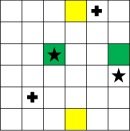
(a) Environment

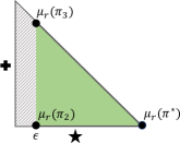
(b) Set of $\mu_{r}(\pi)$ vectors

Figure 1: An illustrative example to showcase the suboptimality of teaching when the learner has preferences and constraints. Environment: Figure 1(a) shows a grid-world environment inspired by the object-world and gathering game environments [Levine et al., 2010, Leibo et al., 2017, Mendez et al., 2018]. Each cell represents a state, there are five actions given by “left", “up", “right", "down", “stay", the transitions are deterministic, and the starting state is the top-left cell. The agent’s goal is to collect objects in the environment: Collecting a “star" provides a reward of $1.0$ and a “plus" a reward of $0.9$; objects immediately appear again upon collection, and the rewards are discounted with $\gamma$ close to 1. The optimal policy $\pi^{*}$ is to go to the nearest “star" and then “stay" there. Preferences: A small number of states in the environment are distractors, depicted by colored cells in Figure 1(a). We consider a learner who prefers to avoid “green" distractors: it has a hard constraint that the probability of having a “green" distractor within a $3\textnormal{x}3$ neighborhood, i.e., 1-cell distance, is at most $\epsilon=0.1$. Feature expectation vectors: Figure 1(b) shows the set of feature expectation vectors $\{\mu_{r}({\pi}):\pi\in\Pi\}$. The $x$-axis and the $y$-axis represent the discounted feature count for collecting “star" and “plus" objects, respectively. The striped region represents policies that are feasible w.r.t. the learner’s constraint. Suboptimality of teaching: Upon receiving demonstrations from an optimal policy $\pi^{*}$ with feature vector $\mu_{r}({\pi^{*}})$, the learner under its preference constraint can best match the teacher’s demonstrations (in a sense of minimizing $\|\mu_{r}(\pi^{{\mathsf{L}}})-\mu_{r}(\pi^{*})\|_{2}$) by outputting a policy with $\mu_{r}(\pi_{2})$, which is clearly suboptimal w.r.t. the true rewards. Policy $\pi_{3}$ with feature vector $\mu_{r}({\pi_{3}})$ represents an alternate teaching policy which would have led to higher reward for the learner.

Key challenges in teaching a learner with preference constraints. In this paper, we study a novel setting where the learner has its own preferences which it additionally takes into consideration when learning a policy $\pi^{\mathsf{L}}$ using teacher’s demonstrations. We formally specify our learner model in the next section; here we highlight the key challenges that arise in teaching such a learner. Given that the learner’s primary goal is no longer just imitating the teacher via feature matching, the learner’s output policy can be suboptimal with respect to the true reward even if it had access to $\mu_{r}(\pi^{*})$, i.e., the feature expectation vector of an optimal policy $\pi^{*}$. Figure 1 provides an illustrative example to showcase the suboptimality of teaching when the learner has preferences and constraints. The key challenge that we address in this paper is that of designing a teaching algorithm that selects demonstrations while accounting for the learner’s preferences.

3 Learner Model

In this section we describe the learner models we consider, including different ways of defining preferences and constraints. First, we introduce some notation and definitions that will be helpful. We capture learner’s preferences via a feature map $\phi_{c}:\mathcal{S}\rightarrow[0,1]^{d_{c}}$. We define $\phi(s)$ as a concatenation of the two feature maps $\phi_{r}(s)$ and $\phi_{c}(s)$ given by $[\phi_{r}(s)^{\dagger},\phi_{c}(s)^{\dagger}]^{\dagger}$ and let $d=d_{r}+d_{c}$. Similar to the map $\mu_{r}$, we define $\mu_{c}\colon\Pi\to\mathbb{R}^{d_{c}}$, $\pi\mapsto\mathbb{E}\left(\sum_{t=0}^{\infty}\gamma^{t}\phi_{c}(s_{t})\right)$ and $\mu\colon\Pi\to\mathbb{R}^{d}$, $\pi\mapsto\mathbb{E}\left(\sum_{t=0}^{\infty}\gamma^{t}\phi(s_{t})\right)$. Similar to $\Omega_{r}$, we define $\Omega_{c}\subseteq\mathbb{R}^{d_{c}}$ and $\Omega\subseteq\mathbb{R}^{d}$ as the images of the maps $\mu_{c}(\Pi)$ and $\mu(\Pi)$. Note that for any policy $\pi\in\Pi$, we have $\mu(\pi)=[\mu_{r}(\pi)^{\dagger},\mu_{c}(\pi)^{\dagger}]^{\dagger}$.

Standard (discounted) MCE-IRL. Our learner models build on the (discounted) Maximum Causal Entropy (MCE) IRL framework [Ziebart et al., 2008, Ziebart, 2010, Ziebart et al., 2013, Zhou et al., 2018]. In the standard (discounted) MCE-IRL framework, a learning agent aims to identify a policy that matches the feature expectations of the teacher’s demonstrations while simultaneously maximizing the (discounted) causal entropy given by $H(\pi):=H(\{a_{t}\}_{t=0,1,\ldots}\|\{s_{t}\}_{t=0,1,\ldots}):=\sum_{t=0}^{\infty}\gamma^{t}\mathbb{E}\Big{[}-\log\pi(a_{t}\mid s_{t})\Big{]}$. More background is provided in Appendix D.

Including preference constraints. The standard framework can be readily extended to include learner’s preferences in the form of constraints on the preference features $\phi_{c}$. Clearly, the learner’s preferences can render exact matching of the teacher’s demonstrations infeasible and hence we relax this condition. To this end, we consider the following generic learner model:

$$\max_{\pi,\ \delta^{\textnormal{soft}}_{r}\geq 0,\ \delta^{\textnormal{soft}}_{c}\geq 0}\quad H(\pi)-C_{r}\cdot\|\delta^{\textnormal{soft}}_{r}\|_{p}-C_{c}\cdot\|\delta^{\textnormal{soft}}_{c}\|_{p}$$ (1)

s.t. $$\lvert\mu_{r}(\pi)[i]-\hat{\mu}_{r}(\Xi^{\mathsf{T}})[i]\rvert\leq\delta^{\textnormal{hard}}_{r}[i]+\delta^{\textnormal{soft}}_{r}[i]\ \forall i\in\{1,2,\ldots,d_{r}\}$$

$$\qquad\qquad\quad g_{j}(\mu_{c}(\pi))\leq\delta^{\textnormal{hard}}_{c}[j]+\delta^{\textnormal{soft}}_{c}[j]\ \forall j\in\{1,2,\ldots,m\},$$

Here, $g\colon\mathbb{R}^{d_{c}}\mapsto\mathbb{R}$ are $m$ convex functions representing preference constraints. The coefficients $C_{r}$ and $C_{c}$ are the learner’s parameters which quantify the relative importance of matching the teacher’s demonstrations and satisfying the learner’s preferences. The learner model is further characterized by parameters $\delta^{\textnormal{hard}}_{r}[i]$ and $\delta^{\textnormal{hard}}_{c}[j]$ (we will use the vector notation as $\delta^{\textnormal{hard}}_{r}\in\mathbb{R}^{d_{r}}_{\geq 0}$ and $\delta^{\textnormal{hard}}_{c}\in\mathbb{R}^{m}_{\geq 0}$). The optimization variables for the learner are given by $\pi$, $\delta^{\textnormal{soft}}_{r}[i]$, and $\delta^{\textnormal{soft}}_{c}[j]$ (we will use the vector notation as $\delta^{\textnormal{soft}}_{r}\in\mathbb{R}^{d_{r}}_{\geq 0}$ and $\delta^{\textnormal{soft}}_{c}\in\mathbb{R}^{m}_{\geq 0}$). These parameters ($\delta_{r}^{\textnormal{hard}}$, $\delta_{c}^{\textnormal{hard}}$) and optimization variables ($\delta_{r}^{\textnormal{soft}}$, $\delta_{c}^{\textnormal{soft}}$) characterize the following behavior:

• While a mismatch of up to $\delta_{r}^{\textnormal{hard}}$ between the learner’s and teacher’s reward feature expectations incurs no cost regarding the optimization objective, a mismatch larger than $\delta_{r}^{\textnormal{hard}}$ incurs a cost of $C_{r}\cdot\|\delta_{r}^{\textnormal{soft}}\|_{p}$.

• Similarly, while a violation of up to $\delta_{c}^{\textnormal{hard}}$ of the learner’s preference constraints incurs no cost regarding the optimization objective, a violation larger than $\delta_{c}^{\textnormal{hard}}$ incurs a cost of $C_{c}\cdot\|\delta_{c}^{\textnormal{soft}}\|_{p}$.

Next, we discuss two special instances of this generic learner model.

3.1 Learner Model with Hard Preference Constraints

It is instructive to study a special case of the above-mentioned generic learner model. Let us consider the model in Eq. 1 with $\delta^{\textnormal{hard}}_{r}=0,\delta^{\textnormal{hard}}_{c}=0$, and a limiting case with $C_{r},C_{c}\gg 0$ such that the term $H(\pi)$ can be neglected. Now, if we additionally assume that $C_{c}\gg C_{r}$, the learner’s objective can be thought of as finding a policy $\pi$ that minimizes the $L^{p}$ norm distance to the reward feature expectations of the teacher’s demonstration while satisfying the constraints $g_{j}(\mu_{c}(\pi))\leq 0\ \forall j\in\{1,2,\ldots,m\}$. More formally, we study the following learner model given in Eq. 2 below:

$$\min_{\pi}\quad \|\mu_{r}(\pi)-\hat{\mu}_{r}(\Xi^{\mathsf{T}})\|_{p}$$ (2)

s.t. $$g_{j}(\mu_{c}(\pi))\leq 0\ \forall j\in\{1,2,\ldots,m\}.$$

To get a better understanding of the model, we can define the learner’s constraint set as $\Omega^{\mathsf{L}}:=\{\mu:\mu\in\Omega\textnormal{ s.t. }g_{j}(\mu_{c})\leq 0\ \forall j\in\{1,2,\ldots,m\}\}$. Similar to $\Omega^{\mathsf{L}}$, we define $\Omega^{\mathsf{L}}_{r}\subseteq\Omega_{r}$ where $\Omega^{\mathsf{L}}_{r}$ is the projection of the set $\Omega^{\mathsf{L}}$ to the subspaces $\mathbb{R}^{d_{r}}$. We can now rewrite the above optimization problem as $\min_{\pi\colon\mu_{r}(\pi)\in\Omega^{\mathsf{L}}_{r}}\|\mu_{r}(\pi)-\hat{\mu}_{r}(\Xi^{\mathsf{T}})\|_{p}$. Hence, the learner’s behavior is given by:

1. Learner can match: When $\hat{\mu}_{r}(\Xi^{\mathsf{T}})\in\Omega_{r}^{\mathsf{L}}$, the learner outputs a policy $\pi^{\mathsf{L}}$ s.t. $\mu_{r}(\pi^{\mathsf{L}})=\hat{\mu}_{r}(\Xi^{\mathsf{T}})$.

2. Learner cannot match: Otherwise, the learner outputs a policy $\pi^{\mathsf{L}}$ such that $\mu_{r}(\pi^{\mathsf{L}})$ is given by the $L^{p}$ norm projection of the vector $\hat{\mu}_{r}(\Xi^{\mathsf{T}})$ onto the set $\Omega_{r}^{\mathsf{L}}$.

Figure 1 provides an illustration of the behavior of this learner model. We will design learner-aware teaching algorithms for this learner model in Section 4.1 and Section 5.

3.2 Learner Model with Soft Preference Constraints

Another interesting learner model that we study in this paper arises from the generic learner when we consider $m=d_{c}$ number of box-type linear constraints with $g_{j}(\mu_{c}(\pi))=\mu_{c}(\pi)[j]\ \forall j\in\{1,2,\ldots,d_{c}\}$. We consider an $L^{1}$ norm penalty on violation, and for simplicity we consider $\delta^{\textnormal{hard}}_{r}[i]=0\ \forall i\in\{1,2,\ldots,d_{r}\}$. In this case, the learner’s model is given by

$$\max_{\pi,\ \delta^{\textnormal{soft}}_{r}\geq 0,\ \delta^{\textnormal{soft}}_{c}\geq 0}\quad H(\pi)-C_{r}\cdot\|\delta^{\textnormal{soft}}_{r}\|_{1}-C_{c}\cdot\|\delta^{\textnormal{soft}}_{c}\|_{1}$$ (3)

s.t. $$\lvert\mu_{r}(\pi)[i]-\hat{\mu}_{r}(\Xi^{\mathsf{T}})[i]\rvert\leq\delta^{\textnormal{soft}}_{r}[i]\ \forall i\in\{1,2,\ldots,d_{r}\}$$

$$\qquad\quad\quad\ \ \ \ \ \mu_{c}(\pi)[j]\leq\delta^{\textnormal{hard}}_{c}[j]+\delta^{\textnormal{soft}}_{c}[j]\ \forall j\in\{1,2,\ldots,d_{c}\},$$

The solution to the above problem corresponds to a softmax policy with a reward function $R_{\bm{\lambda}}(s)=\langle\bm{w}_{\bm{\lambda}},\phi(s)\rangle$ where $\bm{w}_{\bm{\lambda}}\in\mathbb{R}^{d}$ is parametrized by $\bm{\lambda}$. The optimal parameters $\bm{\lambda}$ can be computed efficiently and the corresponding softmax policy is then obtained by Soft-Value-Iteration procedure (see [Ziebart, 2010, Algorithm. 9.1], [Zhou et al., 2018]). Details are provided in Appendix E. We will design learner-aware teaching algorithms for this learner model in Section 4.2.

4 Learner-aware Teaching under Known Constraints

In this section, we analyze the setting when the teacher has full knowledge of the learner’s constraints.

4.1 A Learner-aware Teacher for Hard Preferences: Aware-CMDP

Here, we design a learner-aware teaching algorithm when considering the learner from Section 3.1. Given that the teacher has full knowledge of the learner’s preferences, it can compute an optimal teaching policy by maximizing the reward over policies that satisfy the learner’s preference constraints, i.e., the teacher solves a constrained-MDP problem (see [De, 1960, Altman, 1999]) given by

$$\max_{\pi}\quad \langle\mathbf{w}_{r}^{*},\mu_{r}(\pi)\rangle\quad\textnormal{s.t.}\quad\mu_{r}(\pi)\in\Omega^{\mathsf{L}}_{r}.$$

We refer to an optimal solution of this problem as $\pi^{\textnormal{aware}}$ and the corresponding teacher as Aware-CMDP. We can make the following observation formalizing the value of learner-aware teaching:

Theorem 1.

For simplicity, assume that the teacher can provide an exact feature expectation $\mu(\pi)$ of a policy instead of providing demonstrations to the learner. Then, the value of learner-aware teaching is

$$\max_{\pi\textnormal{ s.t. }\mu_{r}(\pi)\in\Omega^{\mathsf{L}}_{r}}\Big{\langle}\mathbf{w}_{r}^{*},\mu_{r}(\pi)\Big{\rangle}-\Big{\langle}\mathbf{w}_{r}^{*},\textnormal{Proj}_{\Omega^{\mathsf{L}}_{r}}\big{(}\mu_{r}(\pi^{*})\big{)}\Big{\rangle}\geq 0.$$

When the set $\Omega^{\mathsf{L}}$ is defined via a set of linear constraints, the above problem can be formulated as a linear program and solved exactly. Details are provided in Appendix F.

4.2 A Learner-aware Teacher for Soft Preferences: Aware-BiL

For the learner models in Section 3, the optimal learner-aware teaching problem can be naturally formalized as the following bi-level optimization problem:

$$\max_{\pi^{\mathsf{T}}}\quad R(\pi^{\mathsf{L}})\quad\textnormal{s.t.}\quad\pi^{\mathsf{L}}\in\arg\max_{\pi}\textnormal{IRL}(\pi,\mu(\pi^{\mathsf{T}})),$$ (4)

where $\textnormal{IRL}(\pi,\mu(\pi^{\mathsf{T}}))$ stands for the IRL problem solved by the learner given demonstrations from $\pi^{\mathsf{T}}$ and can include preferences of the learner (see Eq. 1 in Section 3).

There are many possibilities for solving this bi-level optimization problem—see for example [Sinha et al., 2018] for an overview. In this paper we adopted a single-level reduction approach to simplify the above bi-level optimization problem as this results in particularly intuitive optimiziation problems for the teacher. The basic idea of single-level reduction is to replace the lower-level problem, i.e., $\arg\max_{\pi}\textnormal{IRL}(\pi,\mu(\pi^{\mathsf{T}}))$, by the optimality conditions for that problem given by the Karush-Kuhn-Tucker conditions [Boyd and Vandenberghe, 2004, Sinha et al., 2018]. For the learner model outlined in Section 3.2, these reductions take the following form (see Appendix G for details):

$$\max_{\bm{\lambda}:=\{\bm{\alpha}^{\textnormal{low}}\in\mathbb{R}^{d_{r}},\ \bm{\alpha}^{\textnormal{up}}\in\mathbb{R}^{d_{r}},\ \bm{\beta}\in\mathbb{R}^{d_{c}}\}}\quad \langle\mathbf{w}_{r}^{*},\mu_{r}(\pi_{\bm{\lambda}})\rangle$$ (5)

s.t. $$0\leq\bm{\alpha}^{\textnormal{low}}\leq C_{r}$$

$$0\leq\bm{\alpha}^{\textnormal{up}}\leq C_{r}$$

$$\{0\leq\bm{\beta}\leq C_{c}\texttt{\ AND\ }\mu_{c}(\pi_{\bm{\lambda}})\leq\delta_{c}^{\textnormal{hard}}\} \texttt{\ OR\ }\{\bm{\beta}=C_{c}\texttt{\ AND\ }\mu_{c}(\pi_{\bm{\lambda}})\geq\delta_{c}^{\textnormal{hard}}\}$$

where $\pi_{\bm{\lambda}}$ corresponds to a softmax policy with a reward function $R_{\bm{\lambda}}(s)=\langle\bm{w}_{\bm{\lambda}},\phi(s)\rangle$ for $\bm{w}_{\bm{\lambda}}=[(\bm{\alpha}^{\textnormal{low}}-\bm{\alpha}^{\textnormal{up}})^{\dagger},-\bm{\beta}^{\dagger}]^{\dagger}$. Thus, finding optimal demonstrations means optimization over softmax teaching policies while respecting the learner’s preferences. To actually solve the above optimization problem and find good teaching policies, we use an approach inspired by the Frank-Wolfe algorithm [Jaggi, 2013] detailed in Appendix G. We refer to a teacher implementing this approach as Aware-BiL.

5 Learner-Aware Teaching Under Unknown Constraints

In this section, we consider the more realistic and challenging setting in which the teacher $\mathsf{T}$ does not know the learner $\mathsf{L}$’s constraint set $\Omega_{r}^{\mathsf{L}}$. Without feedback from $\mathsf{L}$, $\mathsf{T}$ can generally not do better than the agnostic teacher who simply ignores any constraints. We therefore assume that $\mathsf{T}$ and $\mathsf{L}$ interact in rounds as described by Algorithm 1. The two versions of the algorithm we describe in Sections 5.1 and 5.2 are obtained by specifying how $\mathsf{T}$ adapts the teaching policy in each round.

Algorithm 1 Teacher-learner interaction in the adaptive teaching setting

1:Initial teaching policy $\pi^{\mathsf{T},0}$ (e.g., optimal policy ignoring any constraints)

2:for round $i=0,1,2,\dots$ do

3:     Teacher provides demonstrations with feature vector $\mu_{r}^{\mathsf{T},i}$ using policy $\pi^{\mathsf{T},i}$

4:     Learner upon receiving $\mu_{r}^{\mathsf{T},i}$ computes a policy $\pi^{\mathsf{L},i}$ with feature vector $\mu_{r}^{\mathsf{L},i}$

5:     Teacher observes learner’s feature vector $\mu_{r}^{\mathsf{L},i}$ and adapts the teaching policy

In this section, we assume that $\mathsf{L}$ is as described in Section 3.1: Given demonstrations $\Xi^{\mathsf{T}}$, $\mathsf{L}$ finds a policy $\pi^{\mathsf{L}}$ such that $\mu_{r}(\pi^{\mathsf{L}})$ matches the $L^{2}$-projection of $\hat{\mu}_{r}(\Xi^{\mathsf{T}})$ onto $\Omega^{\mathsf{L}}_{r}$. For the sake of simplifying the presentation and the analysis, we also assume that $\mathsf{L}$ and $\mathsf{T}$ can observe the exact feature expectations of their respective policies, e.g., $\hat{\mu}_{r}(\Xi^{\mathsf{T}})=\mu_{r}(\pi^{\mathsf{T}})$ if $\Xi^{\mathsf{T}}$ is sampled from $\pi^{\mathsf{T}}$.

5.1 An Adaptive Learner-aware Teacher Using Volume Search: AdAware-Vol

In our first adaptive teaching algorithm AdAware-Vol, $\mathsf{T}$ maintains an estimate $\hat{\Omega}_{r}^{\mathsf{L}}\supset\Omega_{r}^{\mathsf{L}}$ of the learner’s constraint set, which in each round gets updated by intersecting the current version with a certain affine halfspace, thus reducing the volume of $\hat{\Omega}_{r}^{\mathsf{L}}$. The new teaching policy is then any policy $\pi^{\mathsf{T},i+1}$ which is optimal under the constraint that $\mu^{\mathsf{T},i+1}\in\hat{\Omega}_{r}^{\mathsf{L}}$. The interaction ends as soon as $\lVert\mu^{\mathsf{L},i}_{r}-\mu^{\mathsf{T},i}_{r}\rVert_{2}\leq\epsilon$ for a threshold $\epsilon$. Details are provided in Appendix C.1.

Theorem 2.

Upon termination of AdAware-Vol, $\mathsf{L}$’s output policy $\pi^{\mathsf{L}}$ satisfies $R(\pi^{\mathsf{L}})\geq R(\pi^{\textnormal{aware}})-\epsilon$ for any policy $\pi^{\textnormal{aware}}$ which is optimal under $\mathsf{L}$’s constraints. For the special case that $\Omega^{\mathsf{L}}_{r}$ is a polytope defined by $m$ linear inequalities, the algorithm terminates in $O(m^{d_{r}})$ iterations.

5.2 An Adaptive Learner-aware Teacher Using Line Search: AdAware-Lin

In our second adaptive teaching algorithm, AdAware-Lin, $\mathsf{T}$ adapts the teaching policy by performing a binary search on a line segment of the form $\{\mu_{r}^{\mathsf{L},i}+\alpha\mathbf{w}_{r}^{*}~{}|~{}\alpha\in[\alpha_{\min},\alpha_{\max}]\}\subset\mathbb{R}^{d_{r}}$ to find a vector $\mu_{r}^{\mathsf{T},i+1}=\mu_{r}^{\mathsf{L},i}+\alpha_{i}\mathbf{w}_{r}^{*}$ that is the vector of feature expectations of a policy; here $\alpha_{\max}>\alpha_{\min}>0$ are fixed constants. If that is not successful, the teacher finds a teaching policy with $\mu_{r}^{\mathsf{T},i+1}\in\mathop{\rm arg\,min}_{\mu_{r}\in\Omega_{r}}\|\mu_{r}-\mu_{r}^{\mathsf{L},i}-\alpha_{\min}\mathbf{w}_{r}^{*}\|_{2}$. The following theorem analyzes the convergence of $\mathsf{L}$’s performance to $\overline{R}_{\mathsf{L}}:=\max_{\mu_{r}\in\Omega_{r}}R(\mu_{r})$ under the assumption that $\mathsf{T}$’s search succeeds in every round. The proof and further details are provided in Appendix C.2.

Theorem 3.

Fix some $\varepsilon>0$ and assume that there exists a constant $\alpha_{\min}>0$ such that, as long as $\overline{R}_{\mathsf{L}}-R(\mu_{r}^{\mathsf{L},i})>\varepsilon$, the teacher can find a teaching policy $\pi^{\mathsf{T},i+1}$ satisfying $\mu_{r}^{\mathsf{T},i+1}=\mu_{r}^{\mathsf{L},i}+\alpha_{i}\mathbf{w}_{r}^{*}$ for some $\alpha_{i}\geq\alpha_{\min}$. Then the learner’s performance increases monotonically in each round of AdAware-Lin, i.e., $R(\mu_{r}^{\mathsf{L},i+1})>R(\mu_{r}^{\mathsf{L},i})$. Moreover, after at most $O(\frac{D^{2}}{\varepsilon\alpha_{\min}}\log\frac{D}{\varepsilon})$ teaching steps, the learner’s performance satisfies $R(\mu_{r}^{\mathsf{L},i})>\overline{R}_{\mathsf{L}}-2\varepsilon$. Here we abbreviate $D:=\operatorname{diam}\Omega_{r}$.

6 Experimental Evaluation

In this section we evaluate our teaching algorithms for different types of learners on the environment introduced in Figure 1. The environment we consider here has three types of reward objects, i.e., a “star" object with reward of $1.0$, a “plus" object with reward of $0.9$, and a “dot" object with reward of $0.2$. Two objects of each type are placed randomly on the grid such that there is always only a single object in each grid cell. The presence of an object of type “star”, “plus”, or “dot” in some state $s$ is encoded in the reward features $\phi_{r}(s)$ by a binary-indicator for each type such that $d_{r}=3$. We use a discount factor of $\gamma=0.99$. Upon collecting an object, there is a $0.1$ probability of transiting to a terminal state.

Learner models. We consider a total of 5 different learners whose preferences can be described by distractors in the environment. Each learner prefers to avoid a certain subset of these distractors. There is a total of 4 of distractors: (i) two “green" distractors are randomly placed at a distance of 0-cell and 1-cell to the “star" objects, respectively; (ii) two “yellow" distractors are randomly placed at a distance of 1-cell and 2-cells to the “plus" objects, respectively, see Figure 2(a).

Through these distractors we define learners L1-L5 as follows: (L1) no preference features ($d_{c}=0$); (L2) two preference features ($d_{c}=2$) such that $\phi_{c}(s)[1]$ and $\phi_{c}(s)[2]$ are binary indicators of whether there is a “green" distractor at a distance of 0-cells or 1-cell, respectively; (L3) four preference features ($d_{c}=4$) such that $\phi_{c}(s)[1],\phi_{c}(s)[2]$ are as for L2, and $\phi_{c}(s)[3]$ and $\phi_{c}(s)[4]$ are binary indicators of whether there is a “green" distractor at a distance of 2-cells or a “yellow” distractor at a distance of 0-cells, respectively; (L4) five preference features ($d_{c}=5$) such that $\phi_{c}(s)[1],\ldots,\phi_{c}(s)[4]$ are as for L3, and $\phi_{c}(s)[5]$ is a binary indicator whether there is a “yellow” distractor at a distance of 1-cell; and (L5) six preference features ($d_{c}=6$) such that $\phi_{c}(s)[1],\ldots,\phi_{c}(s)[5]$ are as for L4, and $\phi_{c}(s)[6]$ is a binary indicator whether there is a “yellow” distractor at a distance of 2-cells.

The first row in Figure 2 shows an instance of the considered object-worlds and indicates the preference of the learners to avoid certain regions by the gray area.

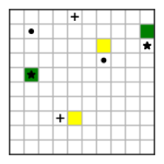
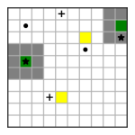
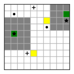
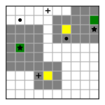
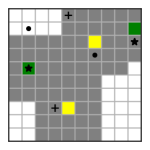
(a) Environments and learners’ preferences for 5 different learners L1, $\ldots$, L5

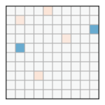
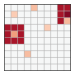
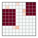
(b) Learners’ rewards inferred from learner-agnostic teacher’s (Agnostic) demonstrations

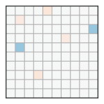
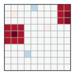
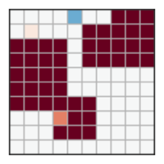
(c) Learners’ rewards inferred from learner-aware teacher’s (Aware-BiL) demonstrations

Figure 2: Teaching in object-world environments under full knowledge of the learner’s preferences. Green and yellow cells indicate distractors associated with either “star" or “plus" objects, respectively. Learner’s preferences to avoid cells are indicated in gray. Learner model from Section 3.2 with $C_{r}=5$, $C_{c}=10$, and $\delta^{\textnormal{hard}}_{c}=0$ is considered for these experiments. The learner-aware teacher enable the learner to infer reward functions that are compatible with the learner’s preferences and achieve higher average rewards. In Figure 2(b) and Figure 2(c), blue color represents positive reward, red color represents negative reward, and the magnitude of the reward is indicated by color intensity.

6.1 Teaching under known constraints

In this section we consider learners with soft constraints from Section 3.2, with preference features as described above, and parameters $C_{r}=5$, $C_{c}=10$, and $\delta^{\textnormal{hard}}_{c}=0$ (more experimental results for different values of $C_{r}$ and $C_{c}$ are provided in Appendix B.1). Our first results are presented in Figure 2. The second and third rows show the rewards inferred by the learners for demonstrations provided by a learner-agnostic teacher who ignores any constraints (Agnostic) and the bi-level learner-aware teacher (Aware-BiL), respectively. We observe that Agnostic fails to teach the learner about objects’ positive rewards in cases where the learners’ preferences conflict with the position of the most rewarding objects (second row). In contrast, Aware-BiL always successfully teaches the learners about rewarding objects that are compatible with the learners’ preferences (third row).

We also compare Agnostic and Aware-BiL in terms of reward achieved by the learner after teaching for object worlds of size $10\times 10$ in Table 1. The numbers show the average reward over 10 randomly generated object-worlds. Note that Aware-BiL has to solve a non-convex optimization problem to find the optimal teaching policy, cf. Eq. 5. Because we use a gradient-based optimization approach, the teaching policies found can depend on the initial point for optimization. Hence, we always consider the following two initial points for optimization and select the teaching policy which results in a higher objective value: (i) all optimization variables in Eq. 5 are set to zero, and (ii) the optimization variables are initialized as $\alpha^{\textnormal{low}}[i]=\max\{w_{\bm{\lambda}}[i],0\}$, $\alpha^{\textnormal{up}}[i]=\max\{-w_{\bm{\lambda}}[i],0\}$, and $\bm{\beta}=0$, where $\bm{w}_{\bm{\lambda}}$ is as inferred by the learner when taught by Agnostic and $i\in\{1,\ldots,d_{r}\}$, cf. Section 3.2. From Table 1 we observe that a learner can learn better policies from a teacher that accounts for the learner’s preferences.

Table 1: Learners’ average rewards after teaching. L1, $\ldots$, L5 correspond to learners with preferences as shown in Figure 2. Results are averaged over 10 random object-worlds, $\pm$ standard error

		Learner ($C_{r}=5,C_{c}=10$)
		L1	L2	L3	L4	L5
Teacher	Agnostic	$7.99\pm 0.02$	$0.01\pm 0.00$	$0.01\pm 0.00$	$0.01\pm 0.00$	$0.00\pm 0.00$
	Aware-BiL	$8.00\pm 0.02$	$7.20\pm 0.01$	$4.86\pm 0.30$	$3.15\pm 0.27$	$1.30\pm 0.07$

6.2 Teaching under unknown constraints

In this section we evaluate the teaching algorithms from Section 5. We consider the learner model from Section 3.1 that uses $L^{2}$-projection to match reward feature expectations as studied in Section 5, cf. Eq. 2. For modeling the hard constraints, we consider box-type linear constraints with $\delta^{\textnormal{hard}}_{c}[j]=2.5\ \forall j\in\{1,2,\ldots,d_{c}\}$ for the preference features, cf. Eq. 3.

We study the learners L1, L2, and L3 with preferences corresponding to the first three object-worlds shown in Figure 2(a). We report the results for learner L2 below; results for learners L1 and L3 are deferred to the Appendix B.2.

In this context it is instructive to investigate how quickly these adaptive teaching strategies converge to the performance of a teacher who has full knowledge about the learner. Results comparing the adaptive teaching strategies (AdAware-Vol and AdAware-Lin) are shown in Figure 3(a). We can observe that both teaching strategies get close to the best possible performance under full knowledge about the learner (Aware-CMDP). We also provide results showing the performance achieved by the adaptive teaching strategies on object-worlds of varying sizes, see Figure 3(b).

Note that the performance of AdAware-Vol decreases slightly when teaching for more rounds, i.e., comparing the results after 3 teaching rounds and at the end of the teaching process. This is because of approximations when learner is computing the policy via projection, which in turn leads to errors on the teacher side when approximating $\hat{\Omega}_{r}^{\mathsf{L}}$ (refer to discussion in Footnote 1). In contrast, AdAware-Lin performance always increases when teaching for more rounds.

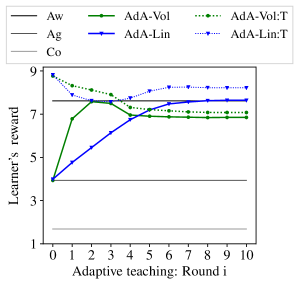
(a) Reward over teaching rounds

	$10\times 10$	$15\times 15$	$20\times 20$
Aware-CMDP	$7.62\pm 0.02$	$7.44\pm 0.04$	$7.19\pm 0.04$
Agnostic	$3.94\pm 0.09$	$3.84\pm 0.06$	$3.95\pm 0.06$
Conserv	$1.68\pm 0.01$	$1.67\pm 0.012$	$1.62\pm 0.02$
AdAware-Vol ($3^{\textnormal{rd}}$)	$7.50\pm 0.14$	$7.50\pm 0.04$	$7.29\pm 0.05$
AdAware-Vol (end)	$6.85\pm 0.33$	$7.06\pm 0.06$	$6.77\pm 0.08$
AdAware-Lin ($3^{\textnormal{rd}}$)	$6.14\pm 0.08$	$6.28\pm 0.10$	$6.37\pm 0.08$
AdAware-Lin (end)	$7.64\pm 0.02$	$7.53\pm 0.03$	$7.29\pm 0.06$

(b) Varying grid-size

Figure 3: Performance of adaptive teaching strategies AdAware-Vol and AdAware-Lin. (left) Figure 3(a) shows the reward for learner’s policy over number of teaching interactions. The horizontal lines indicate the performance of learner’s policy for the learner-aware teacher with full knowledge of the learner’s constraints Aware-CMDP, the learner-agnostic teacher Agnostic who ignores any constraints, and a conservative teacher Conserv who considers all $6$ constraints (assuming the learner model L5 in Figure 2). Our adaptive teaching strategies AdAware-Vol and AdAware-Lin significantly outperform baselines (Agnostic and Conserv) and quickly converge towards the optimal performance of Aware-CMDP. The dotted lines AdAware-Vol:T and AdAware-Lin:T show the rewards corresponding to teacher’s policy at a round and are shown to highlight the very different behavior of two adaptive teaching strategies. (right) Table 3(b) shows results for varying grid-size of the environment. Results are reported at $i=3^{\textnormal{rd}}$ round and at the “end" round when algorithm reaches it’s stopping criterion. Results are reported as average over 10 runs $\pm$ standard error, where each run corresponds to a random environment.

7 Related Work

Our work is closely related to algorithmic machine teaching [Goldman and Kearns, 1995, Zhu, 2015, Zhu et al., 2018], whose general goal is to design teaching algorithms that optimize the data that is provided to a learning algorithm. Most works in machine teaching so far focus on supervised learning tasks and assume that the learning algorithm is fully known to the teacher, see e.g., [Zhu, 2013, Singla et al., 2014, Liu and Zhu, 2016, Mac Aodha et al., 2018].

In the IRL setting, few works study how to provide maximally informative demonstrations to the learner, e.g., [Cakmak and Lopes, 2012, Brown and Niekum, 2019]. In contrast to our work, their teacher fully knows the learner model and provides the demonstrations without any adaptation to the learner. The question of how a teacher should adaptively react to a learner has been addressed by [Singla et al., 2013, Liu et al., 2018, Chen et al., 2018, Melo et al., 2018, Yeo et al., 2019, Hunziker et al., 2019], but only in the supervised setting. In a recent work, [Kamalaruban et al., 2019] have studied the problem of adaptively teaching an IRL agent by providing an informative sequence of demonstrations. However, they assume that the teacher has full knowlege of the learner’s dynamics.

Within the area of IRL, there is a line of work on active learning approaches [Cohn et al., 2011, Brown et al., 2018, Brown and Niekum, 2018, Amin et al., 2017, Cui and Niekum, 2018], which is related to our work. In contrast to us, they take the perspective of the learner who actively influences the demonstrations it receives. A few papers have addressed the problem that arises when the learner does not have full access to the reward features, e.g., [Levine et al., 2010] and [Haug et al., 2018].

Our work is also loosely related to multi-agent reinforcement learning. [Dimitrakakis et al., 2017] studied the interaction between agents with misaligned models with a focus on the question of how to jointly optimize a policy. [Ghosh et al., 2019] studied the problem of designing robust AI agent that can interact with another agent of unknown type. However, these works do not tackle the problem of teaching an agent by demonstrations. Another related work is [Hadfield-Menell et al., 2016] which studied the cooperation of agents who do not perfectly understand each other.

8 Conclusions and Outlook

In this paper we considered inverse reinforcement learning in the context of learners with preferences and constraints. In this setting, the learner does not only focus on matching the teacher’s demonstrated behavior but also takes its own preferences, e.g., behavioral biases or physical constraints, into account. We developed a theoretical framework for this setting, and proposed and studied algorithms for learner-aware teaching in which the teacher accounts for the learner’s preferences for the cases of known and unknown preference constraints. We demonstrated significant performance improvements of our learner-aware teaching strategies as compared to learner-agnostic teaching both theoretically and empirically. Our theoretical framework and our proposed algorithms foster the application of IRL in real-world settings in which the learner does not blindly follow a teacher’s demonstrations.

There are several promising directions for future work, including but not limited to: The evaluation of our approach in machine-human and human-machine tasks; extensions of our approach to other learner models; approaches for learning efficiently from a learner’s point of view from a fixed set of (potentially suboptimal) demonstrations in the case of preference constraints.

Acknowledgements

This work was supported by Microsoft Research through its PhD Scholarship Programme.

Appendix A List of Appendices

In this section we provide a brief description of the content provided in the appendices of the paper.

• Appendix B provides additional experimental results (Section 6).

• Appendix C provides additional details on the adaptive teaching strategies (Section 5).

• Appendix D provides background on the (discounted) MCE-IRL problem (Section 3).

• Appendix E provides additional details on the (discounted) MCE-IRL problem with preferences (Section 3.2).

• Appendix F provides the LP formulation for the teacher Aware-CMDP (Section 4.1).

• Appendix G provides additional details on the bi-level optimization approach for the teacher Aware-BiL (Section 4.2).

Appendix B Experimental Evaluation: Additional Results (Section 6)

B.1 Teaching under known constraints (Section 6.1)

Additional results for teaching under known constraints are presented in Table 2. We observe that Aware-BiL clearly outperforms Agnostic for most combinations of $C_{r}$ and $C_{c}$. Only for $C_{r}=10,C_{c}=1$, the teachers Aware-BiL and Agnostic achieve similar performance because $C_{r}\gg C_{c}$, and hence the learner values achieving higher reward more than satisfying its preferences.

Table 2: Learners’ average rewards after teaching. L1, $\ldots$, L5 correspond to learners with preferences as shown in Figure 2. Results are averaged over 10 random object-worlds, $\pm$ standard error

		Learner ($C_{r}=5,C_{c}=10$)
		L1	L2	L3	L4	L5
Teacher	Agnostic	$7.99\pm 0.02$	$0.01\pm 0.00$	$0.01\pm 0.00$	$0.01\pm 0.00$	$0.00\pm 0.00$
	Aware-BiL	$8.00\pm 0.02$	$7.20\pm 0.01$	$4.86\pm 0.30$	$3.15\pm 0.27$	$1.30\pm 0.07$

		Learner ($C_{r}=10,C_{c}=10$)
		L1	L2	L3	L4	L5
Teacher	Agnostic	$8.34\pm 0.01$	$0.17\pm 0.02$	$0.01\pm 0.00$	$0.01\pm 0.00$	$0.00\pm 0.00$
	Aware-BiL	$8.33\pm 0.01$	$6.90\pm 0.17$	$5.03\pm 0.31$	$3.27\pm 0.28$	$1.35\pm 0.07$

		Learner ($C_{r}=10,C_{c}=5$)
		L1	L2	L3	L4	L5
Teacher	Agnostic	$8.36\pm 0.01$	$8.14\pm 0.03$	$0.01\pm 0.00$	$0.01\pm 0.00$	$0.00\pm 0.00$
	Aware-BiL	$8.34\pm 0.01$	$8.13\pm 0.03$	$5.20\pm 0.29$	$3.43\pm 0.27$	$1.69\pm 0.0$

		Learner ($C_{r}=5,C_{c}=5$)
		L1	L2	L3	L4	L5
Teacher	Agnostic	$7.99\pm 0.02$	$0.17\pm 0.02$	$0.01\pm 0.00$	$0.01\pm 0.00$	$0.00\pm 0.00$
	Aware-BiL	$8.00\pm 0.02$	$6.64\pm 0.17$	$4.87\pm 0.30$	$3.16\pm 0.27$	$1.31\pm 0.06$

		Learner ($C_{r}=10,C_{c}=1$)
		L1	L2	L3	L4	L5
Teacher	Agnostic	$8.36\pm 0.01$	$8.39\pm 0.02$	$8.46\pm 0.02$	$8.46\pm 0.02$	$8.49\pm 0.02$
	Aware-BiL	$8.33\pm 0.01$	$8.36\pm 0.03$	$8.44\pm 0.02$	$8.44\pm 0.02$	$8.46\pm 0.02$

		Learner ($C_{r}=1,C_{c}=10$)
		L1	L2	L3	L4	L5
Teacher	Agnostic	$5.67\pm 0.02$	$0.15\pm 0.02$	$0.16\pm 0.02$	$0.11\pm 0.01$	$0.08\pm 0.01$
	Aware-BiL	$5.93\pm 0.02$	$4.49\pm 0.15$	$3.56\pm 0.24$	$2.30\pm 0.22$	$0.93\pm 0.05$

B.2 Teaching under unknown constraints (Section 6.2)

Here, we provide additional experimental results for teaching algorithms from Section 5. In particular, we report on the results for learner L1 and learner L3, similar to the results for learner L2 reported in Section 6.2.

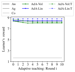
(a) Reward over teaching rounds

	$10\times 10$	$15\times 15$	$20\times 20$
Aware-CMDP	$8.42\pm 0.03$	$8.24\pm 0.05$	$7.84\pm 0.08$
Agnostic	$8.42\pm 0.03$	$8.24\pm 0.05$	$7.84\pm 0.08$
Conserv	$1.68\pm 0.1$	$1.66\pm 0.01$	$1.65\pm 0.02$
AdAware-Vol ($3^{\textnormal{rd}}$)	$8.04\pm 0.02$	$7.83\pm 0.04$	$7.46\pm 0.07$
AdAware-Vol (end)	$8.06\pm 0.02$	$7.80\pm 0.08$	$7.30\pm 0.12$
AdAware-Lin ($3^{\textnormal{rd}}$)	$8.44\pm 0.04$	$8.23\pm 0.07$	$8.08\pm 0.08$
AdAware-Lin (end)	$8.44\pm 0.04$	$8.23\pm 0.07$	$8.08\pm 0.08$

(b) Varying grid-size

Figure 4: Results for learner L1

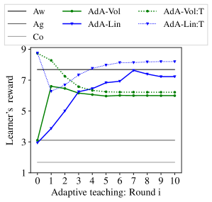
(a) Reward over teaching rounds

	$10\times 10$	$15\times 15$	$20\times 20$
Aware-CMDP	$7.68\pm 0.04$	$7.35\pm 0.03$	$7.39\pm 0.09$
Agnostic	$3.11\pm 0.08$	$3.12\pm 0.07$	$3.26\pm 0.14$
Conserv	$1.68\pm 0.01$	$1.65\pm 0.01$	$1.62\pm 0.01$
AdAware-Vol ($3^{\textnormal{rd}}$)	$6.16\pm 0.42$	$5.72\pm 0.54$	$6.39\pm 0.32$
AdAware-Vol (end)	$5.99\pm 0.46$	$5.38\pm 0.56$	$6.16\pm 0.31$
AdAware-Lin ($3^{\textnormal{rd}}$)	$6.25\pm 0.20$	$5.13\pm 0.50$	$6.15\pm 0.11$
AdAware-Lin (end)	$7.22\pm 0.16$	$5.83\pm 0.62$	$7.09\pm 0.07$

(b) Varying grid-size

Figure 5: Results for learner L3

Appendix C Details for Learner-Aware Teaching under Unknown Constraints (Section 5)

In this appendix, we provide more details on the adaptive teaching algorithms AdAware-Vol and AdAware-Lin described in Sections 5.1 and 5.2. Recall that both teaching algorithms are obtained from Algorithm 1 by defining the way in which the teacher $\mathsf{T}$ adapts the teaching policy based on the learner $\mathsf{L}$’s feature expectations $\mu_{r}^{\mathsf{L}}$ in past rounds.

C.1 Details for AdAware-Vol (Section 5.1)

Estimation of the learner’s constraint set.

In AdAware-Vol, $\mathsf{T}$ maintains an estimate $\hat{\Omega}_{r}^{\mathsf{L},i}$ of $\mathsf{L}$’s constraint set, starting with $\hat{\Omega}_{r}^{\mathsf{L},0}=\Omega_{r}$. After observing the feature expectations $\mu_{r}^{\mathsf{L},i}$ of the policy $\mathsf{L}$ found in round $i$, $\mathsf{T}$ updates this estimate as follows:

$$\hat{\Omega}_{r}^{\mathsf{L},i+1}~{}:=~{}\hat{\Omega}_{r}^{\mathsf{L},i}\cap\{\mu_{r}^{\mathsf{L},i}+\nu\in\mathbb{R}^{d_{r}}~{}|~{}\langle\mu_{r}^{\mathsf{T},i}-\mu_{r}^{\mathsf{L},i},\nu\rangle\leq 0\}$$ (6)

The set on the right hand side of (6) with which $\Omega_{r}^{\mathsf{L},i}$ gets intersected is a halfspace containing $\Omega_{r}^{\mathsf{L}}$. This is due to the fact that $\Omega_{r}^{\mathsf{L}}$ is convex by assumption, and to our assumption that $\mathsf{L}$’s learning algorithm is such that it outputs a policy whose feature expectations $\mu_{r}^{\mathsf{L},i}$ match the $L^{2}$-projection of $\mu_{r}^{\mathsf{T},i}$ to $\Omega_{r}^{\mathsf{L}}$. Inductively, it follows that $\hat{\Omega}_{r}^{\mathsf{L},i}\supset\Omega_{r}^{\mathsf{L}}$ for all $i$.

In practice, we implement a slightly modified version of the update step in which we intersect $\hat{\Omega}_{r}^{\mathsf{L},i}$ with a halfspace that is shifted in the direction of $\mu_{r}^{\mathsf{T},i}-\mu_{r}^{\mathsf{L},i}$ by a small amount, i.e., we use

$$\{\mu_{r}^{\mathsf{L},i}+(1-\eta)(\mu_{r}^{\mathsf{T},i}-\mu_{r}^{\mathsf{L},i})+\nu\in\mathbb{R}^{d_{r}}~{}|~{}\langle\mu_{r}^{\mathsf{T},i}-\mu_{r}^{\mathsf{L},i},\nu\rangle\leq 0\}$$

with a step size parameter $\eta\in(0,1)$. This helps make the algorithm more robust to noise in the learner’s feature expectations. In our experiments, we used $\eta=0.9$.

Update of the teaching policy.

After updating the estimate of the learner’s constraint set to $\hat{\Omega}_{r}^{\mathsf{L},i}$, $\mathsf{T}$ solves a constrained MDP in order to find

$$\pi^{\mathsf{T},i+1}\in\mathop{\rm arg\,max}_{\pi,\mu_{r}(\pi)\in\hat{\Omega}_{r}^{\mathsf{L},i}}R(\pi).$$

Given that $\hat{\Omega}_{r}^{\mathsf{L},i}$ is cut out by linear equations, solving the constrained MDP reduces to solving an LP, as described in Appendix F.

Termination of the interaction.

The algorithm terminates as soon as the stopping criterion $\|\mu_{r}^{\mathsf{L},i}-\mu_{r}^{\mathsf{T},i}\|_{2}\leq\epsilon$ is satisfied. Note that $\hat{\Omega}_{r}^{\mathsf{L},i}\supset\Omega_{r}^{\mathsf{L}}$ implies that

$$R(\pi^{\mathsf{T},i})\geq R(\pi^{\textnormal{aware}})$$

for any $\pi^{\textnormal{aware}}\in\mathop{\rm arg\,max}_{\pi,\mu_{r}(\pi)\in\Omega_{r}^{\mathsf{L}}}R(\pi)$. Therefore, after termination we have

$$R(\pi^{\mathsf{L},i})\geq R(\pi^{\textnormal{aware}})-\epsilon$$

for any policy $\pi^{\textnormal{aware}}$ which is optimal under $\mathsf{L}$’s constraints, which is the first statement of Theorem 2.

The second statement of Theorem 2 follows from the fact that if $\Omega_{r}^{\mathsf{L}}$ is a convex polytope cut out by $m$ linear inequalities, the number of faces, which is in $O(m^{d_{r}})$, is an upper bound on the number of iterations of the algorithm, because one face is “eliminated” in each round.

C.2 Details for AdAware-Lin (Section 5.2)

Algorithm 2 LineSearch

1:$\mu_{r}^{\mathsf{L}}$, $\alpha_{\min}$, $\alpha_{\max}$, $\varepsilon_{\alpha}$, $\varepsilon_{\mu}$.

2:$\alpha_{u}\leftarrow\alpha_{\max}$, $\alpha_{l}\leftarrow\alpha_{\min}$

3:while $\alpha_{u}-\alpha_{l}>\varepsilon_{\alpha}$ do

4:     $\alpha\leftarrow(\alpha_{u}+\alpha_{l})/2$

5:     $\pi^{\mathsf{T}}\leftarrow\textsc{IRL}(\mu_{r}^{\mathsf{L}}+\alpha\mathbf{w}_{r}^{*})$

6:     if $\|\mu_{r}(\pi^{\mathsf{T}})-\mu_{r}^{\mathsf{L}}-\alpha\mathbf{w}_{r}^{*}\|_{2}>\varepsilon_{\mu}$ then

7:         $\alpha_{u}\leftarrow\alpha$

8:     else

9:         $\alpha_{l}\leftarrow\alpha$      

10:if $\|\mu_{r}(\pi^{\mathsf{T}})-\mu_{r}^{\mathsf{L}}-\alpha\mathbf{w}_{r}^{*}\|_{2}>\varepsilon_{\mu}$ then

11:     $\pi^{\mathsf{T}}\leftarrow\textsc{IRL}(\mu_{r}^{\mathsf{L}}+\alpha_{\min}\mathbf{w}_{r}^{*})$

12:return $\pi^{\mathsf{T}}$

Figure 6:

LineSearch is the algorithm that $\mathsf{T}$ uses in order to find a teaching policy $\pi^{\mathsf{T}}$ provided that the feature expectations of $\mathsf{L}$’s current policy are $\mu_{r}^{\mathsf{L}}$. Figure 6 illustrates the two cases may occur: For the right $\mu_{r}^{\mathsf{L}}$, LineSearch returns a policy $\pi^{\mathsf{T}}$ whose feature expectations satisfy $\mu_{r}^{\mathsf{T}}=\mu_{r}^{\mathsf{L}}+\alpha^{*}\mathbf{w}_{r}^{*}$ such that $\alpha^{*}>\alpha_{\min}$. For the left $\mu_{r}^{\mathsf{L}}$, LineSearch returns a policy $\pi^{\mathsf{T}}$ whose feature expectations satisfy $\mu_{r}^{\mathsf{T}}\in\mathop{\rm arg\,min}_{\mu_{r}\in\Omega_{r}}\|\mu_{r}-\mu_{r}^{\mathsf{L}}+\alpha_{\min}\mu_{r}^{\mathsf{T}}\|$.

In AdAware-Lin, $\mathsf{T}$ updates the teaching policy $\pi^{\mathsf{T},i+1}$ based on $\mathsf{L}$’s feature expectations $\mu_{r}^{\mathsf{L},i}$ from the previous round. To do so, $\mathsf{T}$ uses LineSearch (Algorithm 2) to perform a binary search on the line segment

$$\{\mu_{r}^{\mathsf{L},i}+\alpha\mathbf{w}_{r}^{*}~{}|~{}\alpha\in[\alpha_{\min},\alpha_{\max}]\}\subset\mathbb{R}^{d_{r}}$$ (7)

in order to find a vector $\mu_{r}$ that is realizable as the vector of feature expectations of a policy. If the intersection of the line segment (7) with $\Omega_{r}$ is non-empty, it is of the form $\{\mu_{r}^{\mathsf{L}}+\alpha\mathbf{w}_{r}^{*}~{}|~{}\alpha\in[\alpha_{\min},\alpha^{*}]\}$ for some $\alpha^{*}\leq\alpha_{\max}$ due to the convexity of $\Omega_{r}$. In that case, LineSearch returns a policy with feature expectations

$$\mu_{r}^{\mathsf{T},i+1}=\mu_{r}^{\mathsf{L},i}+\alpha_{i}^{*}\mathbf{w}_{r}^{*},$$

where $\alpha_{i}^{*}$ is the maximal $\alpha\in[\alpha_{\min},\alpha_{\max}]$ such that $\mu_{r}^{\mathsf{L},i}+\alpha\mathbf{w}_{r}^{*}\in\Omega_{r}$. If the intersection is empty, LineSearch returns a policy with feature expectations

$$\mu_{r}^{\mathsf{T},i+1}\in\mathop{\rm arg\,min}_{\mu_{r}\in\Omega_{r}}\|\mu_{r}-\mu_{r}^{\mathsf{L},i}-\alpha_{\min}\mathbf{w}_{r}^{*}\|_{2}.$$

Figure 6 illustrates the two cases that may occur.

C.2.1 Proof of Theorem 3

In this section, we provide the proof of Theorem 3, which gives a guarantee on the improvement of $\mathsf{L}$’s performance in each round of the AdAware-Lin algorithm. The assumption we make here is that, in every teaching round, LineSearch returns a teaching policy $\pi^{\mathsf{T},i+1}$ such that $\mu_{r}^{\mathsf{T},i+1}=\mu_{r}^{\mathsf{L},i}+\alpha_{i}\mathbf{w}_{r}^{*}$ for some $\alpha_{i}\geq\alpha_{\min}$, where $\alpha_{\min}>0$ is a fixed constant. It is easy to see that this assumption, together with our assumption on $\mathsf{L}$’s algorithm and the convexity of $\Omega_{r}^{\mathsf{L}}$, imply that the change in learner performance

$$\Delta R_{i}:=R(\mu_{r}^{\mathsf{L},i+1})-R(\mu_{r}^{\mathsf{L},i})$$

is non-negative in every teaching round. The following proposition, which will be needed in the proof of Theorem 3, strengthens this statement:

Proposition 1.

Let $\overline{R}_{\mathsf{L}}:=\max_{\mu_{r}\in\Omega_{r}^{\mathsf{L}}}R(\mu_{r})$ be the maximally achievable learner performance. Assume that, in teaching round $i$, $\mathsf{T}$ can find a teaching policy $\pi^{\mathsf{T},i+1}$ whose feature expectations satisfy $\mu_{r}^{\mathsf{T},i+1}=\mu_{r}^{\mathsf{L},i}+\alpha_{i}\mathbf{w}_{r}^{*}$ for some $\alpha_{i}>0$. Then

$$\overline{R}_{\mathsf{L}}-R(\mu_{r}^{\mathsf{L},i})\leq\Delta R_{i}+D\cdot\sqrt{\frac{\Delta R_{i}}{\alpha_{i}-\Delta R_{i}}},$$ (8)

where $D=\operatorname{diam}\Omega_{r}$.

Proof of Proposition 1.

Consider the plane $V\subset\mathbb{R}^{d_{r}}$ spanned by $\mu_{r}^{\mathsf{L},i},\mu_{r}^{\mathsf{T},i+1}$ and $\mu_{r}^{\mathsf{L},i+1}$ and denote by $\tilde{\mu}_{r}$ the unique point in $V$ with the properties that

1. $\langle\mathbf{w}_{r}^{*},\tilde{\mu}_{r}\rangle=\langle\mathbf{w}_{r}^{*},\mu_{r}^{\mathsf{L},i+1}\rangle$,

2. $\tilde{\mu}_{r}$ lies on the same side of the line through $\mu^{\mathsf{L},i}$ and $\mu^{\mathsf{T},i+1}$ as $\mu_{r}^{\mathsf{L},i+1}$, and

3. $\tilde{\mu}_{r},\mu_{r}^{\mathsf{T},i+1}$ and $\mu_{r}^{\mathsf{L},i}$ span a right triangle with $\tilde{\mu}_{r}$ at the right-angled corner.

Note that $\mu_{r}^{\mathsf{L},i+1}$ must lie inside this triangle, i.e., on the red line segment in Figure 7: Otherwise there would a point on the line segment connecting $\mu_{r}^{\mathsf{L},i+1}$ and $\mu_{r}^{\mathsf{L},i}$, and hence in $\Omega_{r}^{\mathsf{L}}$ by convexity, which is closer to $\mu_{r}^{\mathsf{T},i+1}$ than $\mu_{r}^{\mathsf{L},i+1}$, contradicting the fact that $\mu_{r}^{\mathsf{L},i+1}$ is closest to $\mu_{r}^{\mathsf{T},i+1}$ among all points in $\Omega_{r}^{\mathsf{L}}$. Denote by $\tilde{\ell}$ the line passing through $\tilde{\mu}_{r}$ and $\mu_{r}^{\mathsf{L},i}$.

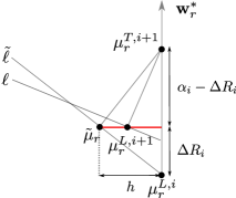
Figure 7: Illustration of the proof of Proposition 1: The smaller the performance increase $\Delta R_{i}$, the better the upper bound on the gap $\overline{R}_{\Omega}-R(\mu_{r}^{\mathsf{L},i})$.

The facts that $\Omega_{r}^{\mathsf{L}}$ is convex and that $\mu_{r}^{\mathsf{L},i+1}=\mathop{\rm arg\,min}_{\mu_{r}\in\Omega_{r}^{\mathsf{L}}}\|\mu_{r}^{\mathsf{T},i+1}-\mu_{r}\|_{2}$ imply that $\Omega_{r}^{\mathsf{L}}$ must lie on one side of the hyperplane

$$\mu_{r}^{\mathsf{L},i+1}+(\mu_{r}^{\mathsf{T},i+1}-\mu_{r}^{\mathsf{L},i+1})^{\perp}\subset\mathbb{R}^{d_{r}}.$$

Therefore, we can upper bound $\overline{R}_{\mathsf{L}}$ in terms of the slope $s_{\ell}$ of the line $\ell$ which arises by intersecting that hyperplane with $V$:

$$\overline{R}_{\mathsf{L}}\leq R(\mu_{r}^{\mathsf{L},i+1})+D\cdot s_{\ell}=R(\mu_{r}^{\mathsf{L},i})+\Delta R_{i}+D\cdot s_{\ell}.$$ (9)

Note that the slope $s_{\ell}$ is upper bounded by the slope $s_{\tilde{\ell}}$ of $\tilde{\ell}$. We have $s_{\tilde{\ell}}=\frac{\Delta R_{i}}{h}$, where $h$ is the length of the red line segment in Figure 7, and $h=\sqrt{(\alpha_{i}-\Delta R_{i})\Delta R_{i}}$ by Pythagoras’s theorem. Using that, we obtain

$$s_{\ell}\leq s_{\tilde{\ell}}=\sqrt{\frac{\Delta R_{i}}{\alpha_{i}-\Delta R_{i}}}.$$ (10)

The claimed estimate (8) follows by plugging this upper bound for $s$ into (9) and rearranging. ∎

Proof of Theorem 3.

Proof of Theorem 3.

The fact that $R(\mu_{r}^{\mathsf{L},i+1})>R(\mu_{r}^{\mathsf{L},i})$, which is equivalent to $\Delta R_{i}>0$, follows immediately from Proposition 1.

We now prove the claimed rate of convergence.

First, using Proposition 1, we note that the assumption that $\overline{R}_{\mathsf{L}}-R(\mu_{r}^{\mathsf{L},i})>\varepsilon$ implies that

$$\varepsilon<\Delta R_{i}+D\sqrt{\frac{\Delta R_{i}}{\alpha_{i}-\Delta R_{i}}}.$$ (11)

Using that, we can conclude that

$$\sqrt{\Delta R_{i}}>\min\{\sqrt{\varepsilon/2},\varepsilon\sqrt{\alpha_{\min}/(4D^{2}+\varepsilon^{2})}\}.$$ (12)

Indeed, if $\Delta R_{i}\leq\frac{\varepsilon}{2}$, it follows from (11) that we must have $D\cdot\sqrt{\Delta R_{i}/(\alpha_{\min}-\Delta R_{i})}>\frac{\varepsilon}{2}$, which implies $\sqrt{\Delta R_{i}}>\varepsilon\sqrt{\alpha_{\min}/(4D^{2}+\varepsilon^{2})}$. Since we are interested in the behavior as $\varepsilon\to 0$, we assume from now on that $\varepsilon$ is so small that $\varepsilon\sqrt{\alpha_{\min}/(4D^{2}+\varepsilon^{2})}<\sqrt{\varepsilon/2}$, so that (12) becomes

$$\sqrt{\Delta R_{i}}>\varepsilon\sqrt{\alpha_{\min}/(4D^{2}+\varepsilon^{2})}=:C_{0}.$$ (13)

Second, we observe that

$$\sqrt{\alpha_{i}-\Delta R_{i}}>\sqrt{\frac{\alpha_{\min}}{2}}=:C_{1}$$ (14)

except in at most $N:=\frac{2}{\alpha_{\min}}(\max R|_{\Omega}-\min R|_{\Omega})$ teaching steps. To see that, note that if the claimed inequality, which is equivalent to $\alpha_{i}-\frac{\alpha_{\min}}{2}>\Delta R_{i}$, does not hold, performance increases by at least $\Delta R_{i}\geq\frac{\alpha_{\min}}{2}$ as $\alpha_{i}>\alpha_{\min}$, and that can happen at most $N$ times.

The inequalities (13) and (14) together imply that we have

$$C_{0}\cdot C_{1}\leq\sqrt{(\alpha_{i}-\Delta R_{i})\Delta R_{i}}$$ (15)

as long as $\overline{R}_{\mathsf{L}}-R(\mu_{r}^{\mathsf{L},i})>\varepsilon$, except in at most $N$ teaching steps. Setting $C:=\frac{1}{C_{0}\cdot C_{1}}$, this is equivalent to

$$\sqrt{\frac{\Delta R_{i}}{\alpha_{i}-\Delta R_{i}}}\leq C\Delta R_{i}$$ (16)

Plugging (16) into the bound (8) provided by Proposition 1, we obtain the estimate

$$\frac{1}{1+CD}(\overline{R}_{\mathsf{L}}-R(\mu_{r}^{\mathsf{L},i}))\leq\Delta R_{i}.$$ (17)

We have $C=\frac{1}{\varepsilon\alpha_{\min}}\sqrt{2(4D^{2}+\varepsilon^{2})}$, and hence

$$\frac{1}{1+CD}=\frac{\varepsilon\alpha_{\min}}{\varepsilon\alpha_{\min}+\sqrt{2(4D^{2}+\varepsilon^{2})}\cdot D}\geq\frac{1}{1+\sqrt{10}}\frac{\varepsilon\alpha_{\min}}{D^{2}}=:\lambda$$ (18)

If we had the estimates (17), (18) for all teaching steps, we could conclude that the learner performance satisfies $R(\mu_{r}^{\mathsf{L},i})>\overline{R}_{\mathsf{L}}-2\varepsilon$ after at most $O(\frac{D^{2}}{\varepsilon\alpha_{\min}}\log\frac{D}{\varepsilon})$ teaching steps. One can see that e.g. by comparing the sequence $R_{0},R_{1},R_{2},\dots$ with the solution $R(t)$ of the ordinary differential equation $\dot{R}=\lambda(\overline{R}_{\mathsf{L}}-R)$, which satifies $\overline{R}_{\mathsf{L}}-R(t)=(\overline{R}_{\mathsf{L}}-R(0))\exp(-\lambda t)$. Since the number $N$ of teaching steps for which (17), (18) do potentially not hold is $O(\frac{D}{\alpha_{\min}})$, we can still make this conclusion. ∎

Appendix D Background on (discounted) MCE-IRL Problem (Section 3)

Our learner models build on the (discounted) Maximum Causal Entropy (MCE) IRL framework [Ziebart et al., 2008, Ziebart, 2010, Ziebart et al., 2013, Zhou et al., 2018]. The results below are based on the MDCE-IRL formulation from [Zhou et al., 2018].

D.1 Primal problem

In the standard (discounted) MCE-IRL framework, a learning agent aims to identify a policy that matches the feature expectations of the teacher’s demonstrations while simultaneously maximizing the (discounted) causal entropy of the policy, i.e., the learner solves the following optimization problem:

$$\max_{\pi}\quad H^{\gamma}(A_{0:\infty}\|S_{0:\infty}):=\sum_{t=0}^{\infty}\gamma^{t}\mathbb{E}\Big{[}-\log\pi(a_{t}\mid s_{t})\Big{]}$$

subject to $$\mu_{r}(\pi)[i]=\hat{\mu}_{r}(\Xi^{\mathsf{T}})[i]\quad\forall i\in\{1,2,\ldots,d_{r}\}.$$

Here, $\mu_{r}(\pi)[i]$ and $\hat{\mu}_{r}(\Xi^{\mathsf{T}})[i]$ denote the scalar values of the $i^{\textnormal{th}}$ reward feature. The idea is that without any further information beyond the teacher’s demonstrations, the most uncertain solution matching the reward feature expectation of those demonstrations should be preferred.

Formulating this as a minimization problem and spelling out all the constraints, we arrive at the following primal:

$$\underset{\bm{\pi}=\{\pi_{t}\}_{t=0}^{\infty}}{\min}-H^{\gamma}(A_{0:\infty}\|S_{0:\infty})$$

subject to

$$\mu_{r}(\pi_{t})[i]=\hat{\mu}_{r}(\Xi^{\mathsf{T}})[i]\quad\forall i\in\{1,2,\ldots,d_{r}\}$$

$$\pi_{t}(a|s)\geq 0\quad\forall a\in\mathcal{A},s\in\mathcal{S},t\geq 0$$

$$\sum_{a\in\mathcal{A}}\pi_{t}(a|s)=1\quad\forall s\in\mathcal{S},t\geq 0$$

$$\pi_{t}(a|s)=\pi_{t^{\prime}}(a|s)\quad\forall a\in\mathcal{A},s\in\mathcal{S},t\geq 0,t^{\prime}\geq 0$$

The last condition ensures that the policy $\pi$ is stationary.

D.2 Lagrangian relaxation

The Lagrangian relaxation optimization formulation of the above primal problem is given by

$$\mathcal{L}(\bm{\pi},\bm{\lambda},\bm{\psi}) =-H^{\gamma}(A_{0:\infty}\|S_{0:\infty})+\bm{\lambda}^{\dagger}(\hat{\mu}_{r}(\Xi^{\mathsf{T}})-\mu_{r}(\pi_{t}))+\sum_{s,t}\psi_{s,t}(1-\sum_{a\in\mathcal{A}}\pi_{t}(a|s))$$

subject to

$$\pi_{t}(a|s)\geq 0\quad\forall a\in\mathcal{A},s\in\mathcal{S},t\geq 0$$

$$\pi_{t}(a|s)=\pi_{t^{\prime}}(a|s)\quad\forall a\in\mathcal{A},s\in\mathcal{S},t,t^{\prime}\geq 0$$

Here, $\bm{\lambda}\in\mathbb{R}^{d_{r}}$ and $\bm{\psi}=\{\psi_{s,t}\}_{\forall s_{t}}$. Also, $\dagger$ is the transpose operator defined for vectors.

Remark. The Lagrangian relaxation of the optimization problem is not convex in the problem variables because of the term $\bm{\lambda}^{\dagger}(\hat{\mu}_{r}(\Xi^{\mathsf{T}})-\mu_{r}(\pi_{t}))$ in the objective function, which is not convex in the variables $\pi_{t}$. However, it can be shown that strong duality holds for both its dual and primal formulations ([Zhou et al., 2018]). The dual formulation is described in Section D.4.

D.3 Parametric form of the policy

For a given $\bm{\lambda}$, the optimal policy $\pi_{\bm{\lambda}}^{\textnormal{soft}}(a|s)$ is given by

$$\pi_{\bm{\lambda}}^{\textnormal{soft}}(a|s) =\frac{\exp(Q_{\bm{\lambda}}^{\textnormal{soft}}(s,a))}{\exp(V_{\bm{\lambda}}^{\textnormal{soft}}(s))}$$

where the quantities are defined recursively as follows:

$$Q_{\bm{\lambda}}^{\textnormal{soft}}(s,a) =\bm{\lambda}^{\dagger}\mu_{r}({\pi_{\bm{\lambda}}^{\textnormal{soft}}}(a|s))+\gamma\sum_{s^{\prime}\in\mathcal{S}}T(s^{\prime}|s,a)V_{\bm{\lambda}}^{\textnormal{soft}}(s^{\prime})$$

$$V_{\bm{\lambda}}^{\textnormal{soft}}(s) =\text{ log }\sum_{a\in\mathcal{A}}\exp(Q_{\bm{\lambda}}^{\textnormal{soft}}(s,a))$$

This is shown by taking the derivative of the Lagrangian, $\mathcal{L}(\bm{\pi},\bm{\lambda},\bm{\psi})$ w.r.t. the primal variables $\pi_{t}$ and equating it to 0, i.e.,

$$\frac{\partial L(\{\pi_{t}\}_{t=0}^{\infty},\bm{\lambda},\bm{\psi})}{\partial\pi_{t}} =0.$$

For a given $\bm{\lambda}$, the corresponding softmax policy can be obtained by Soft-Value-Iteration procedure (see [Ziebart, 2010, Algorithm. 9.1], [Zhou et al., 2018]).

D.4 Dual problem

For any given $\bm{\lambda},\bm{\psi}$, let $g(\bm{\lambda},\bm{\psi})$ be the optimal value for the optimization problem defined by the Lagrangian relaxation problem in Section D.2. As strong duality holds for the (discounted) MCE-IRL problem and its dual counter part, we solve only the following concave dual problem:

$$\underset{\bm{\lambda}\in\mathbb{R}^{d_{r}},\psi_{s,t}\in\mathbb{R}}{\mathrm{maximize}}\quad g(\bm{\lambda},\bm{\psi})$$

D.5 Gradients for the dual variables

As the dual problem is concave, it can be solved using gradient ascent. The gradients of the dual function described in Section D.4 are given by:

$$\nabla_{\bm{\lambda}}\quad g =\hat{\mu}_{r}(\Xi^{\mathsf{T}})-\mu_{r}(\pi_{\bm{\lambda}}^{\textnormal{soft}})$$

$$\nabla_{\psi_{s,t}}\quad g =1-\sum_{a\in\mathcal{A}}\pi_{\bm{\lambda}}^{\textnormal{soft}}(a|s)$$

Here $\pi_{\bm{\lambda}}^{\textnormal{soft}}$ is the parametric softmax policy described above. The second condition is automatically satisfied because $\pi_{\bm{\lambda}}^{\textnormal{soft}}$ is a probability distribution.

The gradient update rule to compute the optimal $\bm{\lambda}$ is:

$$\bm{\lambda}_{\text{next}}\leftarrow\bm{\lambda}-\eta\cdot\big{(}\mu_{r}(\pi_{\bm{\lambda}}^{\textnormal{soft}})-\hat{\mu}_{r}(\Xi^{\mathsf{T}})\big{)}$$

where $\eta$ is the learning rate.

Appendix E Details of (discounted) MCE-IRL Problem with Preferences (Section 3.2)

Here we present the background of the learner model described in Section 3.2. In this setting, the learner’s preferences are modeled as linear soft constraints with L1 penalties. We consider the minimization variant of the problem. The results in this section follow directly from the analysis of Maximum Entropy Models under different constraints, as presented in [Kazama and Tsujii, 2005, Dudík et al., 2007] when applied to (discounted) MCE-IRL problem [Ziebart et al., 2013, Zhou et al., 2018]. For brevity, redundant details of the derivations are omitted.
The final policy of the learner is given by $\pi_{\bm{\lambda}}^{\text{$\textnormal{soft}$}}$ and is defined in Section E.3.

E.1 Primal problem

The primal problem is given by

$$\underset{\bm{\pi}=\{\pi_{t}\}_{t=0}^{\infty};\ \delta^{\textnormal{soft},\textnormal{low}}_{r},\ \delta^{\textnormal{soft},\textnormal{up}}_{r},\ \delta^{\textnormal{soft},\textnormal{up}}_{c}\geq 0}{\min}-H^{\gamma}(A_{0:\infty}||S_{0:\infty})+\sum_{i=1}^{d_{r}}C_{r}\cdot(\delta_{r}^{\textnormal{soft},\textnormal{low}}[i]+\delta_{r}^{\textnormal{soft},\textnormal{up}}[i])+\sum_{j=1}^{d_{c}}C_{c}\cdot\delta_{c}^{\textnormal{soft},\textnormal{up}}[j]$$

subject to

$$\qquad\hat{\mu}_{r}(\Xi^{\mathsf{T}})[i]-\mu_{r}(\pi_{t})[i]\leq\delta_{r}^{\textnormal{soft},\textnormal{low}}[i]\quad\forall i\in\{1,2,\ldots,d_{r}\}$$

$$\qquad\mu_{r}(\pi_{t})[i]-\hat{\mu}_{r}(\Xi^{\mathsf{T}})[i]\leq\delta_{r}^{\textnormal{soft},\textnormal{up}}[i]\quad\forall i\in\{1,2,\ldots,d_{r}\}$$

$$\qquad\mu_{c}(\pi_{t})[j]\leq\delta_{c}^{\textnormal{hard}}[j]+\delta_{c}^{\textnormal{soft},\textnormal{up}}[j]\quad\forall j\in\{1,2,\ldots,d_{c}\}$$

Here we have $\delta_{r}^{\textnormal{soft},\textnormal{low}},\delta_{r}^{\textnormal{soft},\textnormal{up}}\in\mathbb{R}^{d_{r}}$ and $\delta_{c}^{\textnormal{soft},\textnormal{up}}\in\mathbb{R}^{d_{c}}$ as the primal optimization slack variables with the constraint that $\delta^{\textnormal{soft},\textnormal{low}}_{r},\delta^{\textnormal{soft},\textnormal{up}}_{r},\delta_{c}^{\textnormal{soft},\textnormal{up}}\geq 0$. We also have $C_{r}>0,C_{c}>0$. $\delta_{c}^{\textnormal{hard}}\in\mathbb{R}^{d_{c}}$ is a given constant vector.

Remark. low and up in the superscripts of dual variables represent whether they are variables for lower bound constraints or upper bound constraints.

E.2 Lagrangian relaxation

The Lagrangian relaxation optimization formulation of the primal problem described in Section E.1 is given by

$$\mathcal{L}(\bm{\pi},\delta^{\textnormal{soft},\textnormal{low}}_{r},\delta^{\textnormal{soft},\textnormal{up}}_{r},\delta_{c}^{\textnormal{soft},\textnormal{up}},\bm{\lambda},\bm{\psi}) =-H^{\gamma}(A_{0:\infty},S_{0:\infty})+(\bm{\alpha}^{\textnormal{low}}-\bm{\alpha}^{\textnormal{up}})^{\dagger}(\hat{\mu}_{r}(\Xi^{\mathsf{T}})-\mu_{r}(\pi_{t}))$$

$$+\bm{\beta}^{\dagger}\mu_{c}(\pi_{t})$$

$$+\sum_{s,t}\psi_{s,t}(1-\sum_{a\in\mathcal{A}}\pi_{t}(a|s))-(\bm{\alpha}^{\textnormal{low}})^{\dagger}\delta^{\textnormal{soft},\textnormal{low}}_{r}-(\bm{\alpha}^{\textnormal{up}})^{\dagger}\delta^{\textnormal{soft},\textnormal{up}}_{r}$$

$$-\bm{\beta}^{\dagger}\delta_{c}^{\textnormal{soft},\textnormal{up}}-\bm{\beta}^{\dagger}\delta_{c}^{\textnormal{hard}}$$

$$-(\bm{\rho}^{\textnormal{low}})^{\dagger}\delta_{r}^{\textnormal{soft},\textnormal{low}}-(\bm{\rho}^{\textnormal{up}})^{\dagger}\delta_{r}^{\textnormal{soft},\textnormal{up}}$$

$$-\bm{\sigma}^{\dagger}\delta_{c}^{\textnormal{soft},\textnormal{up}}$$

$$+\sum_{i=1}^{d_{r}}C_{r}\cdot(\delta_{r}^{\textnormal{soft},\textnormal{low}}[i]+\delta_{r}^{\textnormal{soft},\textnormal{up}}[i])+\sum_{j=1}^{d_{c}}C_{c}\cdot\delta_{c}^{\textnormal{soft},\textnormal{up}}[j]$$

subject to

$$\pi_{t}(a|s)\geq 0\quad\forall a\in\mathcal{A},s\in\mathcal{S},t\geq 0$$

$$\pi_{t}(a|s)=\pi_{t^{{}^{\prime}}}(a|s)\quad\forall a\in\mathcal{A},s\in\mathcal{S},t,t^{{}^{\prime}}\geq 0$$

Here, $\bm{\alpha}^{\textnormal{low}},\bm{\alpha}^{\textnormal{up}},\bm{\rho}^{low},\bm{\rho}^{up}\in\mathbb{R}^{d_{r}}$, and $\bm{\beta},\bm{\sigma}\in\mathbb{R}^{d_{c}}$. We also have non-negativity constraints on the dual variables: $\bm{\alpha}^{\textnormal{low}},\bm{\alpha}^{\textnormal{up}},\bm{\beta},\bm{\rho}^{\textnormal{low}},\bm{\rho}^{\textnormal{up}},\bm{\sigma}\geq 0$. A few additional notes:

• For convenience, we will denote the group of dual variables as $\bm{\lambda}:=\{\bm{\alpha}^{\textnormal{low}},\bm{\alpha}^{\textnormal{up}},\bm{\beta},\bm{\rho}^{\textnormal{low}},\bm{\rho}^{\textnormal{up}},\bm{\sigma}\}$

• The reward parameter $\bm{w_{\bm{\lambda}}}=[(\bm{\alpha}^{\textnormal{low}}-\bm{\alpha}^{\textnormal{up}})^{\dagger},-\bm{\beta}^{\dagger}]^{\dagger}$ is used to define the learner’s reward function $R_{\bm{\lambda}}(s)=\langle\bm{w}_{\bm{\lambda}},\phi(s)\rangle$.

• $\dagger$ is the transpose operator, defined for vectors.

E.3 Parametric form of the policy

For a given, $\bm{\lambda}:=\{\bm{\alpha}^{\textnormal{low}},\bm{\alpha}^{\textnormal{up}},\bm{\beta},\bm{\rho}^{\textnormal{low}},\bm{\rho}^{\textnormal{up}},\bm{\sigma}\}$, the optimal policy $\pi_{\bm{\lambda}}^{\textnormal{soft}}(a|s)$ is given by

$$\pi_{\bm{\lambda}}^{\textnormal{soft}}(a|s) =\frac{\exp(Q_{\bm{\lambda}}^{\textnormal{soft}}(s,a))}{\exp(V_{\bm{\lambda}}^{\textnormal{soft}}(s))}$$

where the quantities are defined recursively as follows:

$$Q_{\bm{\lambda}}^{\textnormal{soft}}(s,a) =(\bm{\alpha}_{low}-\bm{\alpha}_{up})^{\dagger}\mu_{r}({\pi_{\bm{\lambda}}^{\textnormal{soft}}}(a|s))-\bm{\beta}^{\dagger}\mu_{c}({\pi_{\bm{\lambda}}^{\textnormal{soft}}}(a|s))+\gamma\sum_{s^{{}^{\prime}}\in\mathcal{S}}T(s^{{}^{\prime}}|s,a)V_{\bm{\lambda}}^{\textnormal{soft}}(s^{{}^{\prime}})$$

$$V_{\bm{\lambda}}^{\textnormal{soft}}(s) =\text{ log }(\sum_{a\in\mathcal{A}}\exp(Q_{\bm{\lambda}}^{\textnormal{soft}}(s,a)))$$

This is shown by taking the derivative of the Lagrangian, $\mathcal{L}(\bm{\pi},\bm{\lambda},\bm{\psi})$ w.r.t the primal variables, $\pi_{t}$ and equating it to 0. i.e.

$$\frac{\partial L(\{\pi_{t}\}_{t=0}^{\infty},\bm{\lambda},\bm{\psi})}{\partial\pi_{t}} =0$$

E.4 Updated Lagrangian

We find the partial derivatives of the Lagrangian defined in Section E.2 w.r.t all the primal variables, $\delta^{\textnormal{soft},\textnormal{low}}_{r},\delta^{\textnormal{soft},\textnormal{up}}_{r},\delta_{c}^{\textnormal{soft},\textnormal{up}}$:

$$\frac{\partial\mathcal{L}}{\partial\delta^{\textnormal{soft},\textnormal{low}}_{r}[i]} =0$$

$$\Rightarrow\alpha^{\textnormal{low}}[i] =C_{r}-\rho^{\textnormal{low}}[i]$$

$$\text{Also, }\frac{\partial\mathcal{L}}{\partial\delta^{\textnormal{soft},\textnormal{up}}_{r}} =0$$

$$\Rightarrow\alpha^{\textnormal{up}}[i] =C_{r}-\rho^{\textnormal{up}}[i]$$

$$\text{And, }\frac{\partial\mathcal{L}}{\partial\delta^{\textnormal{soft},\textnormal{up}}_{c}} =0$$

$$\Rightarrow\beta[i] =C_{r}-\sigma[i]$$

The dual variables satisfy $\bm{\sigma},\bm{\rho}^{\textnormal{low}},\bm{\rho}^{\textnormal{up}}\geq 0$. Hence, the above conditions translate into the following constraints on the set of dual variables, $\bm{\alpha}^{\textnormal{low}},\bm{\alpha}^{\textnormal{up}},\bm{\beta}$:

$$0\leq{\alpha}^{\textnormal{low}}[i]\leq C_{r}\quad\forall i\in\{1,2,\ldots,d_{r}\}$$

$$0\leq{\alpha}^{\textnormal{up}}[i]\leq C_{r}\quad\forall i\in\{1,2,\ldots,d_{r}\}$$

$$0\leq{\beta}[j]\leq C_{c}\quad\forall j\in\{1,2,\ldots,d_{c}\}$$

The updated Lagrangian now has these additional constraints and is given by:

$$\mathcal{L}(\bm{\pi},\delta^{\textnormal{soft},\textnormal{low}}_{r},\delta^{\textnormal{soft},\textnormal{up}}_{r},\delta_{c}^{\textnormal{soft},\textnormal{up}},\bm{\lambda},\bm{\psi}) =-H^{\gamma}(A_{0:\infty},S_{0:\infty})+(\bm{\alpha}^{\textnormal{low}}-\bm{\alpha}^{\textnormal{up}})^{\dagger}(\hat{\mu}_{r}(\Xi^{\mathsf{T}})-\mu_{r}(\pi_{t}))+\bm{\beta}^{\dagger}\mu_{c}(\pi_{t})$$

$$+\sum_{s,t}\psi_{s,t}(1-\sum_{a\in\mathcal{A}}\pi_{t}(a|s))-(\bm{\alpha}^{\textnormal{low}})^{\dagger}\delta^{\textnormal{soft},\textnormal{low}}_{r}-(\bm{\alpha}^{up})^{\dagger}\delta^{\textnormal{soft},\textnormal{up}}_{r}$$

$$-\bm{\beta}^{\dagger}\delta_{c}^{\textnormal{soft},\textnormal{up}}-\bm{\beta}^{\dagger}\delta_{c}^{\textnormal{hard}}$$

$$-(\bm{\rho}^{\textnormal{low}})^{\dagger}\delta_{r}^{\textnormal{soft},\textnormal{low}}-(\bm{\rho}^{\textnormal{up}})^{\dagger}\delta_{r}^{\textnormal{soft},\textnormal{up}}$$

$$-\bm{\sigma}^{\dagger}\delta_{c}^{\textnormal{soft},\textnormal{up}}$$

$$+\sum_{i=1}^{d_{r}}C_{r}\cdot(\delta_{r}^{\textnormal{soft},\textnormal{low}}[i]+\delta_{r}^{\textnormal{soft},\textnormal{up}}[i])+\sum_{j=1}^{d_{c}}C_{c}\cdot\delta_{c}^{\textnormal{soft},\textnormal{up}}[j]$$

subject to

$$\pi_{t}(a|s)\geq 0\quad\forall a\in\mathcal{A},s\in\mathcal{S},t\geq 0$$

$$\pi_{t}(a|s)=\pi_{t^{{}^{\prime}}}(a|s)\quad\forall a\in\mathcal{A},s\in\mathcal{S},t,t^{{}^{\prime}}\geq 0$$

$$0\leq{\alpha}^{\textnormal{low}}[i]\leq C_{r}\quad\forall i\in\{1,2,\ldots,d_{r}\}$$

$$0\leq{\alpha}^{\textnormal{up}}[i]\leq C_{r}\quad\forall i\in\{1,2,\ldots,d_{r}\}$$

$$0\leq{\beta}[j]\leq C_{c}\quad\forall j\in\{1,2,\ldots,d_{c}\}$$

The set of dual variables becomes $\bm{\lambda}:=\{\bm{\alpha}^{\textnormal{low}},\bm{\alpha}^{\textnormal{up}},\bm{\beta}\}$ and $\bm{\psi}=\{\psi_{s,t}\}_{\forall s_{t}}$.

E.5 Dual problem

For any given $\bm{\lambda,\psi}$, let $g(\bm{\lambda,\psi})$ be the optimal value for the Lagrangian relaxation problem. Strong Duality holds for both our primal and dual formulations, and the dual optimal policy is also optimal for the primal formulation. Hence, we solve the concave dual problem, given by

$$\underset{\bm{\alpha}^{\textnormal{low}},\bm{\alpha}^{\textnormal{up}}\in\mathbb{R}^{d_{r}},\bm{\beta}\in\mathbb{R}^{d_{c}},\psi_{s,t}\in\mathbb{R}}{\textnormal{maximize}}\text{ }g(\bm{\lambda},\bm{\psi})$$

subject to

$$\quad 0\leq\bm{\alpha}^{\textnormal{low}}\leq C_{r}$$

$$\quad 0\leq\bm{\alpha}^{\textnormal{up}}\leq C_{r}$$

$$\quad 0\leq\bm{\beta}\leq C_{c}$$

where $\bm{\lambda}:=\{\bm{\alpha}^{\textnormal{low}},\bm{\alpha}^{\textnormal{up}},\bm{\beta}\}$.

E.6 Gradients for the dual problem

As the dual problem is concave, it can be solved using gradient ascent.
Note that,

$$\nabla_{\psi_{s,t}}g =1-\sum_{a\in\mathcal{A}}\pi_{\bm{\lambda}}^{\textnormal{soft}}(a|s)$$

Here $\pi_{\bm{\lambda}}^{\textnormal{soft}}$ is the parametric softmax policy described above. This condition is automatically satisfied because $\pi_{\bm{\lambda}}^{\textnormal{soft}}$ is a probability distribution. For the remaining dual variables, we have the following gradients:

$$\nabla_{\bm{\alpha}^{\textnormal{low}}}\text{ }g =\hat{\mu}_{r}(\Xi^{\mathsf{T}})-\mu_{r}(\pi_{\bm{\lambda}}^{\textnormal{soft}})$$

$$\nabla_{\bm{\alpha}^{\textnormal{up}}}\quad g =\mu_{r}(\pi_{\bm{\lambda}}^{\textnormal{soft}})-\hat{\mu}_{r}(\Xi^{\mathsf{T}})$$

$$\nabla_{\bm{\beta}}\text{ }g =\mu_{c}(\pi_{\bm{\lambda}}^{\textnormal{soft}})$$

The (projected) gradient update rules to compute the optimal value of the dual variables $(\bm{\alpha}^{\textnormal{low}},\bm{\alpha}^{\textnormal{up}},\bm{\beta})$ are given by the following:

$$\bm{\alpha}^{\textnormal{low}}_{\text{next}} \leftarrow\bm{\alpha}^{\textnormal{low}}-\eta\cdot(\mu_{r}(\pi_{\bm{\lambda}}^{\textnormal{soft}})-\hat{\mu}_{r}(\Xi^{\mathsf{T}}))$$

$${\alpha}^{\textnormal{low}}_{\text{next}}[i] \leftarrow\max(0,{\alpha}^{\textnormal{low}}_{\text{next}}[i])\quad\forall i\in\{1,2,\ldots,d_{r}\}$$

$${\alpha}^{\textnormal{low}}_{\text{next}}[i] \leftarrow\min(C_{r},{\alpha}^{\textnormal{low}}_{\text{next}}[i])\quad\forall i\in\{1,2,\ldots,d_{r}\}$$

$$\bm{\alpha}^{\textnormal{up}}_{\text{next}} \leftarrow\bm{\alpha}^{\textnormal{up}}-\eta\cdot(\hat{\mu}_{r}(\Xi^{\mathsf{T}})-\mu_{r}(\pi_{\bm{\lambda}}^{\textnormal{soft}}))$$

$${\alpha}^{\textnormal{up}}_{\text{next}}[i] \leftarrow\max(0,{\alpha}^{\textnormal{up}}_{\text{next}}[i])\quad\forall i\in\{1,2,\ldots,d_{r}\}$$

$${\alpha}^{\textnormal{up}}_{\text{next}}[i] \leftarrow\min(C_{r},{\alpha}^{\textnormal{up}}_{\text{next}}[i])\quad\forall i\in\{1,2,\ldots,d_{r}\}$$

$$\bm{\beta}_{\text{next}} \leftarrow\bm{\beta}-\eta\cdot(-\mu_{c}(\pi_{\bm{\lambda}}^{\textnormal{soft}}))$$

$${\beta}_{\text{next}}[j] \leftarrow\max(0,{\beta}_{\text{next}}[j])\quad\forall j\in\{1,2,\ldots,d_{c}\}$$

$${\beta}_{\text{next}[j]} \leftarrow\min(C_{c},{\beta}_{\text{next}}[j])\quad\forall j\in\{1,2,\ldots,d_{c}\}$$

where $\eta$ is the learning rate.

Appendix F LP Formulation for the Teacher Aware-CMDP (Section 4.1)

The problem of finding optimal learner-aware teaching demonstrations for the learner in Section 3.1 with linear preferences can be formulated as the following linear program (based on the linear programming formulation for solving MDPs [De, 1960]):

$$\max_{z}\quad \sum_{s}\sum_{a}z(s,a)\langle\mathbf{w}_{r}^{*},\phi_{r}(s)\rangle$$ (19)

s.t. $$\sum_{a}z(s^{\prime},a)=(1-\gamma)P_{0}(s^{\prime})+\gamma\sum_{s}\sum_{a}T(s^{\prime}|s,a)z(s,a)\quad\forall s^{\prime}$$ (20)

$$z(s,a)\geq 0\quad\forall s,a$$ (21)

$$\sum_{s}\sum_{a}z(s,a)\phi_{c}(s)[j]\leq\delta^{\textnormal{hard}}_{c}[j]\quad\forall j\in\{1,2,\ldots,d_{c}\}$$ (22)

Here $z$ is a vector of discounted state-action frequencies and $z(s,a)$ refers to state-action frequency for state $s$ and action $a$. The constraints in (22) are the linear preference constraints. From the optimal solution of the LP, an optimal stochastic policy can be extracted by

$$\pi(s,a):=\frac{z(s,a)}{\sum_{a^{\prime}}z(s,a^{\prime})}.$$ (23)

Appendix G Bi-Level Optimization Approach (Section 4.2)

We only show the formalism for the most general bi-level problem for learners with linear preferences.

G.1 Using Dual (discounted) MCE-IRL formulation for the learner model in Section 3.2

The basic bi-level optimization problem that we aim to solve is the following:

$$\max_{\pi^{\mathsf{T}}} \quad R(\pi^{\mathsf{L}})$$

subject to $$\quad\pi^{\mathsf{L}}\in\arg\max_{\pi}\textnormal{IRL}(\pi,\mu(\pi^{\mathsf{T}})).$$

We will replace the lower-level problem, i.e., $\arg\max_{\pi}\textnormal{IRL}(\pi,\mu(\pi^{\mathsf{T}}))$ with its Karush-Kuhn-Tucker conditions [Boyd and Vandenberghe, 2004, Sinha et al., 2018]. The lower-level problem in its dual formulation is given in Appendix E.5.

Omitting details and replacing $R(\pi_{\bm{\lambda}}):=\langle\mathbf{w}_{r}^{*},\mu_{r}(\pi_{\bm{\lambda}})\rangle$, this yields problems of the following form:

$$\max_{\bm{\lambda}} \quad\langle\mathbf{w}_{r}^{*},\mu_{r}(\pi_{\bm{\lambda}})\rangle$$

subject to:

$$\quad 0\leq\bm{\alpha}^{\textnormal{low}}\leq C_{r}$$

$$\quad 0\leq\bm{\alpha}^{\textnormal{up}}\leq C_{r}$$

$$\quad 0\leq\bm{\beta}\leq C_{c}$$

$$\quad\mu_{c}(\pi_{\bm{\lambda}})\leq(\geq)\delta^{\textnormal{hard}}_{c}$$

where $\bm{\lambda}:=\{\bm{\alpha}^{\textnormal{low}},\bm{\alpha}^{\textnormal{up}},\bm{\beta}\}$. Here $\pi_{\bm{\lambda}}$ corresponds to a softmax policy with a reward function $R_{\bm{\lambda}}(s)=\langle\bm{w}_{\bm{\lambda}},\phi(s)\rangle$ for $\bm{w}_{\bm{\lambda}}=[(\bm{\alpha}^{\textnormal{low}}-\bm{\alpha}^{\textnormal{up}})^{\dagger},-\bm{\beta}^{\dagger}]^{\dagger}$. Thus, finding optimal demonstrations means optimization over softmax teaching policies while respecting the learner’s preferences.

G.1.1 Optimal solution

The cases of the above problem we can observe have to be solved separately and the best solution must be picked. That is, we find the following two solutions: (step i) $\bm{\lambda}^{*}_{1}$, and (step ii) $\bm{\lambda}^{*}_{2}$. Then pick the best $\bm{\lambda}^{*}$ in (step iii):

Step i: $\bm{\lambda}^{*}_{1}$ Compute optimal parameters $\bm{\lambda}^{*}_{1}$ by solving the following problem:

$$\max_{\lambda} \quad\langle\mathbf{w}_{r}^{*},\mu_{r}(\pi_{\bm{\lambda}})\rangle$$

subject to:

$$\quad 0\leq\bm{\alpha}^{\textnormal{low}}\leq C_{r}$$

$$\quad 0\leq\bm{\alpha}^{\textnormal{up}}\leq C_{r}$$

$$\quad 0\leq\bm{\beta}\leq C_{c}$$

$$\quad\mu_{c}(\pi_{\bm{\lambda}})\leq\delta^{\textnormal{hard}}_{c}$$

Step ii: $\bm{\lambda}^{*}_{2}$ Compute optimal parameters $\bm{\lambda}^{*}_{2}$ by solving the following problem:

$$\max_{\bm{\lambda}} \quad\langle\mathbf{w}_{r}^{*},\mu_{r}(\pi_{\bm{\lambda}})\rangle$$ (24)

subject to: (25)

$$\quad 0\leq\bm{\alpha}^{\textnormal{low}}\leq C_{r}$$ (26)

$$\quad 0\leq\bm{\alpha}^{\textnormal{up}}\leq C_{r}$$ (27)

$$\quad\bm{\beta}=C_{c}$$ (28)

$$\quad\mu_{c}(\pi_{\bm{\lambda}})\geq\delta^{\textnormal{hard}}_{c}$$ (29)

Step iii: $\bm{\lambda}^{*}$ Pick the best solution as

$$\bm{\lambda}^{*}=\arg\max_{\bm{\lambda}\in\{\bm{\lambda}^{*}_{1},\bm{\lambda}^{*}_{2}\}}\langle\mathbf{w}_{r}^{*},\mu_{r}(\pi_{\bm{\lambda}})\rangle$$

This provides the optimal policy for the teacher. The teacher then computes feature expectation of this policy and provide it to the learner.

G.2 Solving the above problem

We adopt a variant of the Frank-Wolfe algorithm [Jaggi, 2013] to solve the problems of the form:

$$\max_{\bm{\lambda}} \quad R(\pi_{\bm{\lambda}}):=\langle\mathbf{w}_{r}^{*},\mu_{r}(\pi_{\bm{\lambda}})\rangle$$ (30)

subject to: (31)

$$\quad 0\leq\bm{\alpha}^{\textnormal{low}}\leq C_{r}$$ (32)

$$\quad 0\leq\bm{\alpha}^{\textnormal{up}}\leq C_{r}$$ (33)

$$\quad 0\leq\bm{\beta}\leq C_{c}$$ (34)

$$\quad\mu_{c}(\pi_{\bm{\lambda}})\leq(\geq)\delta^{\textnormal{hard}}_{c}$$ (35)

In particular, we take the following steps to optimize the teaching policy $\pi_{\bm{\lambda}}$:

1. Initialization. Find a feasible starting point $\bm{\lambda}_{0}$

2. Optimization. For $t=1,2,\ldots$

   • Compute the gradient $\bm{g}_{t}=[\nabla_{\bm{\lambda}}R(\pi_{\bm{\lambda}})](\bm{\lambda}_{t-1})$ of the objective at $\bm{\lambda}_{t-1}$. In experiments we approximate the gradient using finite-differences.

   • Linearize the constraints $\mu_{c}(\pi_{\bm{\lambda}})\leq(\geq)\delta^{\textnormal{hard}}_{c}$ at $\bm{\lambda}_{t-1}$ as $\bm{b}_{t}+\bm{A}_{t}(\bm{\lambda}-\bm{\lambda}_{t-1})\leq(\geq)\delta^{\textnormal{hard}}_{c}$, where $\bm{b}_{t}=\mu_{c}(\pi_{\bm{\lambda}_{t-1}})$ and $\bm{A}_{t}=[\nabla_{\bm{\lambda}}\mu_{c}(\pi_{\bm{\lambda}})](\bm{\lambda}_{t-1})$. Again, we employ finite-differences to approximate this linearization. Clearly, we can reuse computation from the gradient estimation of the objective here to reduce computational demands.

   • Solve the direction-finding subproblem (a linear problem):

     $$\max_{\bm{\gamma}} \quad\langle\bm{\gamma},\bm{g}_{t}\rangle$$

     subject to:

     $$\quad 0\leq\bm{\alpha}^{\textnormal{low}}\leq C_{r}$$

     $$\quad 0\leq\bm{\alpha}^{\textnormal{up}}\leq C_{r}$$

     $$\quad 0\leq\bm{\beta}\leq C_{c}$$

     $$\quad\bm{b}_{t}+\bm{A}_{t-1}(\bm{\lambda}-\bm{\lambda}_{t-1})\leq(\geq)\delta^{\textnormal{hard}}_{c}$$

     with optimal solution $\bm{\gamma}_{t}^{*}$. Assuming that the linear approximation of the constraints is accurate locally, the directional vector $\bm{d}_{t}=\bm{\gamma}_{t}^{*}-\bm{\lambda}_{t-1}$ is an ascent direction.

   • Perform a line-search from $\bm{\lambda}_{t-1}$ to $\bm{\gamma}_{t}^{*}$ and let $\bm{\lambda}_{t}$ be the point that maximizes the line search.

   • Upon convergence, terminate the For loop.

Upon convergence of the algorithm, the teacher can use the final $\bm{\lambda}_{t}$ for teaching.

Remark. Observe that the above algorithm would reduce to the standard Frank-Wolfe algorithm with line-search in the case of linear inequalities only.

References

• [Abbeel and Ng, 2004] Abbeel, P. and Ng, A. Y. (2004). Apprenticeship learning via inverse reinforcement learning. In ICML.
• [Altman, 1999] Altman, E. (1999). Constrained Markov decision processes, volume 7. CRC Press.
• [Amin et al., 2017] Amin, K., Jiang, N., and Singh, S. P. (2017). Repeated inverse reinforcement learning. In NIPS, pages 1813–1822.
• [Boularias et al., 2011] Boularias, A., Kober, J., and Peters, J. (2011). Relative entropy inverse reinforcement learning. In AISTATS, pages 182–189.
• [Boyd and Vandenberghe, 2004] Boyd, S. and Vandenberghe, L. (2004). Convex optimization. Cambridge university press.
• [Brown et al., 2018] Brown, D. S., Cui, Y., and Niekum, S. (2018). Risk-Aware Active Inverse Reinforcement Learning. In Conference on Robot Learning, pages 362–372.
• [Brown and Niekum, 2018] Brown, D. S. and Niekum, S. (2018). Efficient probabilistic performance bounds for inverse reinforcement learning. In Thirty-Second AAAI Conference on Artificial Intelligence.
• [Brown and Niekum, 2019] Brown, D. S. and Niekum, S. (2019). Machine teaching for inverse reinforcement learning: Algorithms and applications. In AAAI.
• [Cakmak and Lopes, 2012] Cakmak, M. and Lopes, M. (2012). Algorithmic and human teaching of sequential decision tasks. In AAAI.
• [Chen et al., 2018] Chen, Y., Singla, A., Mac Aodha, O., Perona, P., and Yue, Y. (2018). Understanding the role of adaptivity in machine teaching: The case of version space learners. In Advances in Neural Information Processing Systems, pages 1476–1486.
• [Cohn et al., 2011] Cohn, R., Durfee, E., and Singh, S. (2011). Comparing Action-query Strategies in Semi-autonomous Agents. In AAMAS, pages 1287–1288, Richland, SC.
• [Cui and Niekum, 2018] Cui, Y. and Niekum, S. (2018). Active reward learning from critiques. In 2018 IEEE International Conference on Robotics and Automation (ICRA), pages 6907–6914. IEEE.
• [De, 1960] De, G. G. (1960). Les problemes de decisions sequentielles. cahiers du centre d’etudes de recherche operationnelle vol. 2, pp. 161-179.
• [Dimitrakakis et al., 2017] Dimitrakakis, C., Parkes, D. C., Radanovic, G., and Tylkin, P. (2017). Multi-view decision processes: the helper-ai problem. In Advances in Neural Information Processing Systems, pages 5443–5452.
• [Dudík et al., 2007] Dudík, M., Phillips, S. J., and Schapire, R. E. (2007). Maximum entropy density estimation with generalized regularization and an application to species distribution modeling. Journal of Machine Learning Research, 8:1217–1260.
• [Ghosh et al., 2019] Ghosh, A., Tschiatschek, S., Mahdavi, H., and Singla, A. (2019). Towards deployment of robust AI agents for human-machine partnerships. In Workshop on Safety and Robustness in Decision Making (SRDM) at NeurIPS’19.
• [Goldman and Kearns, 1995] Goldman, S. A. and Kearns, M. J. (1995). On the complexity of teaching. Journal of Computer and System Sciences, 50(1):20–31.
• [Hadfield-Menell et al., 2016] Hadfield-Menell, D., Russell, S. J., Abbeel, P., and Dragan, A. (2016). Cooperative inverse reinforcement learning. In NIPS.
• [Haug et al., 2018] Haug, L., Tschiatschek, S., and Singla, A. (2018). Teaching Inverse Reinforcement Learners via Features and Demonstrations. In Advances in Neural Information Processing Systems, pages 8473–8482.
• [Hunziker et al., 2019] Hunziker, A., Chen, Y., Mac Aodha, O., Rodriguez, M. G., Krause, A., Perona, P., Yue, Y., and Singla, A. (2019). Teaching multiple concepts to a forgetful learner. In Advances in Neural Information Processing Systems.
• [Jaggi, 2013] Jaggi, M. (2013). Revisiting Frank-Wolfe: Projection-free sparse convex optimization. In Proceedings of the 30th International Conference on Machine Learning, pages 427–435.
• [Kamalaruban et al., 2019] Kamalaruban, P., Devidze, R., Cevher, V., and Singla, A. (2019). Interactive teaching algorithms for inverse reinforcement learning. In IJCAI, pages 2692–2700.
• [Kazama and Tsujii, 2005] Kazama, J. and Tsujii, J. (2005). Maximum entropy models with inequality constraints: A case study on text categorization. Machine Learning, 60(1-3):159–194.
• [Leibo et al., 2017] Leibo, J. Z., Zambaldi, V., Lanctot, M., Marecki, J., and Graepel, T. (2017). Multi-agent reinforcement learning in sequential social dilemmas. In Proceedings of the 16th Conference on Autonomous Agents and MultiAgent Systems, pages 464–473.
• [Levine et al., 2010] Levine, S., Popovic, Z., and Koltun, V. (2010). Feature construction for inverse reinforcement learning. In NIPS, pages 1342–1350.
• [Liu and Zhu, 2016] Liu, J. and Zhu, X. (2016). The teaching dimension of linear learners. Journal of Machine Learning Research, 17(162):1–25.
• [Liu et al., 2018] Liu, W., Dai, B., li, X., Rehg, J. M., and Song, L. (2018). Towards black-box iterative machine teaching. In ICML.
• [Mac Aodha et al., 2018] Mac Aodha, O., Su, S., Chen, Y., Perona, P., and Yue, Y. (2018). Teaching categories to human learners with visual explanations. In Proceedings of the IEEE Conference on Computer Vision and Pattern Recognition, pages 3820–3828.
• [Melo et al., 2018] Melo, F. S., Guerra, C., and Lopes, M. (2018). Interactive optimal teaching with unknown learners. In IJCAI, pages 2567–2573.
• [Mendez et al., 2018] Mendez, J. A. M., Shivkumar, S., and Eaton, E. (2018). Lifelong inverse reinforcement learning. In Advances in Neural Information Processing Systems, pages 4507–4518.
• [Osa et al., 2018] Osa, T., Pajarinen, J., Neumann, G., Bagnell, J. A., Abbeel, P., Peters, J., et al. (2018). An algorithmic perspective on imitation learning. Foundations and Trends® in Robotics, 7(1-2):1–179.
• [Ratliff et al., 2006] Ratliff, N. D., Bagnell, J. A., and Zinkevich, M. A. (2006). Maximum margin planning. In ICML, pages 729–736.
• [Singla et al., 2013] Singla, A., Bogunovic, I., Bartók, G., Karbasi, A., and Krause, A. (2013). On actively teaching the crowd to classify. In NIPS Workshop on Data Driven Education.
• [Singla et al., 2014] Singla, A., Bogunovic, I., Bartók, G., Karbasi, A., and Krause, A. (2014). Near-optimally teaching the crowd to classify. In ICML.
• [Sinha et al., 2018] Sinha, A., Malo, P., and Deb, K. (2018). A review on bilevel optimization: from classical to evolutionary approaches and applications. IEEE Transactions on Evolutionary Computation, 22(2):276–295.
• [Yeo et al., 2019] Yeo, T., Kamalaruban, P., Singla, A., Merchant, A., Asselborn, T., Faucon, L., Dillenbourg, P., and Cevher, V. (2019). Iterative classroom teaching. In AAAI, pages 5684–5692.
• [Zhou et al., 2018] Zhou, Z., Bloem, M., and Bambos, N. (2018). Infinite time horizon maximum causal entropy inverse reinforcement learning. IEEE Trans. Automat. Contr., 63(9):2787–2802.
• [Zhu, 2013] Zhu, X. (2013). Machine teaching for bayesian learners in the exponential family. In NIPS, pages 1905–1913.
• [Zhu, 2015] Zhu, X. (2015). Machine teaching: An inverse problem to machine learning and an approach toward optimal education. In AAAI, pages 4083–4087.
• [Zhu et al., 2018] Zhu, X., Singla, A., Zilles, S., and Rafferty, A. N. (2018). An Overview of Machine Teaching. arXiv:1801.05927.
• [Ziebart, 2010] Ziebart, B. D. (2010). Modeling purposeful adaptive behavior with the principle of maximum causal entropy. Carnegie Mellon University.
• [Ziebart et al., 2013] Ziebart, B. D., Bagnell, J. A., and Dey, A. K. (2013). The principle of maximum causal entropy for estimating interacting processes. IEEE Transactions on Information Theory, 59(4):1966–1980.
• [Ziebart et al., 2008] Ziebart, B. D., Maas, A. L., Bagnell, J. A., and Dey, A. K. (2008). Maximum entropy inverse reinforcement learning. In AAAI.