Rotating multistate boson stars

Abstract

In this paper, we construct rotating boson stars composed of the coexisting states of two scalar fields, including the ground and first excited states. We show the coexisting phase with both the ground and first excited states for rotating multistate boson stars. In contrast to the solutions of the nodeless boson stars, the rotating boson stars with two states have two types of nodes, including the ${}^{1}S^{2}S$ state and the ${}^{1}S^{2}P$ state. Moreover, we explore the properties of the mass $M$ of rotating boson stars with two states as a function of the synchronized frequency $\omega$, as well as the nonsynchronized frequency $\omega_{2}$. Finally, we also study the dependence of the mass $M$ of rotating boson stars with two states on angular momentum for both the synchronized frequency $\omega$ and the nonsynchronized frequency $\omega_{2}$.

I Introduction

In the mid-1950s, John Wheeler found the classical fields of electromagnetism coupled to the Einstein gravity theory Wheeler:1955zz ; Power:1957zz . In the next half century, Kaup et al. PhysRev.187.1767 replaced electromagnetism with a free, complex scalar field and found Klein–Gordon geons Kaup:1968zz that have become well-known as boson stars (BSs).

Firstly, boson stars that were constructed with fourth and sixth power $|\phi|$-term potentials were considered in Mielke:1981 , and there is a more detailed analysis of a potential with only the quartic term in Ref. 1986PhRvL..57.2485C . Moreover, by using a V-shaped potential proportional to $|\phi|$, one can also find the compact boson stars Hartmann:2012da , and the same V-shaped potential with an additional quadratic massive term has also been studied in Kumar:2015sia . In Ref. Guenther R.L:1995 , the Newtonian boson stars were investigated, and the boson field coupled to an electromagnetic field in Ref. Jetzer P:1989 . Furthermore, the study of boson stars can be extended to the boson nebulae charge Dariescu C:2010 ; Murariu G.:2010 ; Murariu G.:2008 , the charged boson stars with a cosmological constant case Kumar:2016sxx , and the charged, spinning Q-balls case Brihaye:2009dx . In addition, the fermion-boson stars were studied in Refs. Henriques:1989 ; Henriques:1990 ; deSousa:1995ye ; Pisano:1995yk . Most of the studies of the solutions have focused on the model of one scalar hair with the fundamental solutions. Recently, the spherically symmetric, nonrotating boson stars with two coexisting states was discussed in Refs. Bernal:2009zy ; UrenaLopez:2010ur , which combined the ground state with the first excited state, and the study of the case of nonrotating boson stars with two coexisting states can be extended numerically to the phase shift and dynamics Hawley:2002zn , which is the individual particlelike configurations for each complex field case Brihaye:2009yr ; Brihaye:2008cg . Besides, the axisymmetric rotating radially excited boson stars has been studied in Collodel:2017biu and see Ref. Liebling:2012fv for a review.

On other the hand, BSs with a rotation were first studied in the work of Schunck and Mielke Schunck:1996 , and the rotating boson stars in four and five dimensions have been studied in Kan:2016xkn . After that, Yoshida and Eriguchi constructed the highly relativistic spinning BSs 1997PhRvD..56..762Y . Moreover, the study of the spinning BSs solutions can be extended to the quantization condition case Dias:2011at ; Smolic:2015txa , the quartic self-interacting potential as well as the Kerr black hole limit case Herdeiro:2016gxs . The linear stability of boson stars with respect to small oscillations was discussed by Lee and Pang in Lee:1988av ; the study of the stability of boson stars was extended to the quartic and sextic self-interaction term case Kleihaus:2011sx and nonrotating multistate boson stars Bernal:2009zy ; and the catastrophe theory was applied to extract the stable branches of families of boson stars in Kusmartsev:2008py ; Kusmartsev:1992 .

Recently, a class of Kerr black holes with a scalar hair was discussed by Herdeiro and Radu Herdeiro:2015gia ; Herdeiro:2014goa . The stability of a Kerr black hole with a scalar hair can be found in Refs. Ganchev:2017uuo ; Degollado:2018ypf ; Hod:2012px ; Benone:2014ssa . In Refs. Herdeiro:2016tmi ; Delgado:2016jxq ; Herdeiro:2018wvd ; Herdeiro:2018daq the cases of the Proca hair, the Kerr-Newman black hole, nonminimal coupling case, and spinning black holes with a Skyrme hair have been achieved. The study on long-term numerical evolutions of the superradiant instability of a Kerr black hole by East and Pretorius is found in Ref. East:2017ovw . For a deeper analysis of the numerical methods and a review, see Refs.Herdeiro:2015gia ; Herdeiro:2015waa . The family of a rotating Kerr black hole with a synchronised hair exhibits, besides the physical quantities of mass and angular momentum, a conserved Noether charge Q, which is associated with the complex scalar field, $\psi_{n}\sim e^{-iwt+im\varphi}$ (where $n\in\mathbb{N}_{0}$, $m\in\mathbb{Z}^{*}$) where the node number $n$ and azimuthal harmonic index $m$, most of the studies of the solutions of Kerr black holes with scalar hair focused on the model of ground state ($n=0$) and the smallest azimuthal harmonic index ($m=1$). Very recently, a family of the Kerr black holes with an excited state scalar hair ($n\neq 0$) have also been constructed Wang:2018xhw , and the Kerr black holes with odd parity scalar hair case was considered in Kunz:2019bhm in detail. The case of Kerr black holes with synchronized hair and higher azimuthal harmonic index ($m>1$) have also been investigated in Ref. Delgado:2019prc . In addition, the study of the spinning boson stars and hairy black holes is extended to a two-component Friedberg-Lee-Sirlin model coupled to Einstein gravity in four spacetime dimensions Kunz:2019sgn . In the present work, we are interested in rotating multistate boson stars. We would like to know whether or not two scalar hairs can occupy the same state; furthermore, we will construct possible coexisting states, including the ground and first excited states.

The paper is organized as follows. In Sec. II, we introduce the model of the four-dimensional Einstein gravity coupled to two complex massive scalar fields $\psi_{i}$ $(i=1,2)$ and adopt the same axisymmetric metric with Kerr-like coordinates as the ansatz in Ref. Herdeiro:2014goa . In Sec. III, the boundary conditions of the rotating multistate boson stars (RMSBS) are studied. We show the numerical results of the equations of motion and show the characteristics of the ${}^{1}S^{2}S$ state and the ${}^{1}S^{2}P$ state in Sec. IV. We conclude in Sec. V with a discussion and an outline for further work.

II The model setup

We start with the theory of Einstein gravity coupled to two massive complex scalar fields $\psi_{i}$ $(i=1,2)$,

$$S=\int_{\mathcal{M}}\mathrm{d}^{4}x\sqrt{-g}\left(\frac{R}{16\,\pi\,G}-\nabla_{a}\psi_{1}^{*}\nabla^{a}\psi_{1}-\mu_{1}^{2}|\psi_{1}|^{2}-\nabla_{a}\psi_{2}^{*}\nabla^{a}\psi_{2}-\mu_{2}^{2}|\psi_{2}|^{2}\right)\,,$$ (1)

where $\mu_{i}$ $(i=1,2)$ are the mass of two scalar fields, respectively. From henceforth, we will set $G=c=1$. The corresponding equations of motion are given by

$$\frac{R_{ab}}{8\pi}=2\nabla_{(a}\psi_{1}^{*}\nabla_{b)}\psi_{1}+g_{ab}\mu_{1}^{2}\psi_{1}^{*}\psi_{1}+2\nabla_{(a}\psi_{2}^{*}\nabla_{b)}\psi_{2}+g_{ab}\mu_{2}^{2}\psi_{2}^{*}\psi_{2}\,,$$ (2a)

$$\Box\psi_{1}=\mu_{1}^{2}\psi_{1}\,,$$ (2b)

$$\Box\psi_{2}=\mu_{2}^{2}\psi_{2}\,.$$ (2c)

When both of the two scalar fields vanish, the solution of Eq. (2a) has the stationary axisymmetric asymptotically flat black hole with a mass and angular momentum, which is the well-known Kerr black hole. In terms of Boyer-Lindquist coordinates, the Kerr metric reads

$$\mathrm{d}s^{2}=-\frac{\Delta}{\Sigma^{2}}\left(\mathrm{d}t-a\sin^{2}\theta\mathrm{d}\phi\right)^{2}+\frac{\sin^{2}\theta}{\Sigma^{2}}[a\,\mathrm{d}t-(r^{2}+a^{2})\mathrm{d}\phi]^{2}+\Sigma^{2}\left(\mathrm{d}\theta^{2}+\frac{\mathrm{d}r^{2}}{\Delta}\right)\,,$$ (3)

with $\Delta=r^{2}+a^{2}-2\,M\,r$ and $\Sigma^{2}=r^{2}+a^{2}\cos^{2}\theta$. The black hole event horizon is a null hypersurface with $r=r_{+}\equiv M+\sqrt{M^{2}-a^{2}}$, angular velocity $\Omega_{K}=a/(a^{2}+r_{+}^{2})$, and temperature $T_{K}=(r_{+}^{2}-a^{2})/[4\pi r_{+}(r_{+}^{2}+a^{2})]$. The constant $M$ is the black hole mass and $a$ parameterized is the angular momentum via $J=M\,a$.

In Refs. Herdeiro:2014goa ; Herdeiro:2015gia , Herdeiro and Radu constructed a family of boson stars as well as a Kerr black hole with a ground state scalar hair. In order to construct stationary solutions of the RMSBS, we also take the same numerical method with the following ansatz:

$$ds^{2}=e^{2F_{1}}\left(\frac{dr^{2}}{N}+r^{2}d\theta^{2}\right)+e^{2F_{2}}r^{2}\sin^{2}\theta(d\varphi-Wdt)^{2}-e^{2F_{0}}Ndt^{2},$$ (4)

with $N=1-\frac{r_{H}}{r}\ ,$ and the constant $r_{H}$ that is related to event horizon radius. Besides, the ansatz of two complex scalar fields $\psi_{i}$ are given by

$$\psi_{i}=\phi_{i(n)}(r,\theta)e^{i(m_{i}\varphi-\omega_{i}t)},\;\;\;i=1,2,\;\;\;n=0,1,\cdots,\;\;\;m_{i}=\pm 1,\pm 2,\cdots.$$ (5)

Here, we note that the six functions $F_{0}$, $F_{1}$, $F_{2}$, $W$, and $\phi_{i(n)}$ $(i=1,2)$ depend on the radial distance $r$ and polar angle $\theta$. Again, the constants $\omega_{i}$ $(i=1,2)$ are the frequency of the complex scalar field and $m_{i}$ $(i=1,2)$ are the azimuthal harmonic index, respectively. When $\omega_{1}=\omega_{2}=\omega$, the frequency of the scalar field is called the synchronized frequency, while $\omega_{1}\neq\omega_{2}$ is called the nonsynchronized frequency. The subscript $n$ of Eq.(5) is named as the principal quantum number of the scalar field, and $n=0$ is regarded as the ground state and $n\geq 1$ as the excited states. Besides, in the scalar ansatz (5), subscripts $i$ are indicated by two complex scalar fields only.

It is well known that the ground state scalar hair has no node, that is, along the radial $r$ direction, the value of the scalar field has the same sign. For the rotating boson stars with first excited state, we observe that there are two types of nodes, radial and angular nodes. Radial nodes are the points where the value of the scalar field can change sign along the radial $r$ direction, while angular nodes are the points where the value of the scalar field can change sign along the angular $\theta$ direction. Hence, we would like to construct rotating boson stars composed of two coexisting states of the scalar fields, including the ground state and the first excited state.

III Boundary conditions

Before numerically solving the differential equations instead of seeking the analytical solutions, we should obtain the asymptotic behaviors of the metric functions $F_{0}(r,\theta),F_{1}(r,\theta),F_{2}(r,\theta)$, and $W(r,\theta)$ as well as the scalar field $\phi_{i(n)}(r,\theta)$ $(i=1,2)$, which is equivalent to knowing the boundary conditions we need. Considering the properties of the RMSBS, we will still use the boundary conditions by following the same steps as given in Refs. Herdeiro:2014goa ; Herdeiro:2015gia ; Wang:2018xhw .

For rotating axially symmetric boson stars, exploiting the reflection symmetry $\theta\rightarrow\pi-\theta$ on the equatorial plane, it is enough to consider the range $\theta\in[0,\pi/2]$ for the angular variable. At infinity $r\rightarrow\infty$, the boundary conditions are

$$F_{0}=F_{1}=F_{2}=W=\phi_{i(n)}=0,\;\;\;(i=1,2),\;\;\;n=0,1,\cdots,$$ (6)

and we require the boundary conditions,

$$\partial_{\theta}F_{0}(r,0)=\partial_{\theta}F_{1}(r,0)=\partial_{\theta}F_{2}(r,0)=\partial_{\theta}W(r,0)=\phi_{i(n)}(r,0)=0,\;\;\;n=0,1,\cdots,$$ (7)

for $\theta=0$. For odd parity solutions, we have

$$\partial_{\theta}F_{0}(r,\pi/2)=\partial_{\theta}F_{1}(r,\pi/2)=\partial_{\theta}F_{2}(r,\pi/2)=\partial_{\theta}W(r,\pi/2)=\phi_{i(n)}(r,\pi/2)=0,\;\;\;n=1,2,\cdots,$$ (8)

for $\theta=\pi/2$, while for even parity solutions, $\partial_{\theta}\phi_{i(n)}(r,\pi/2)=0$ with $n=1,2,\cdots$.

For rotating multistate boson stars solutions with $r_{H}=0$,

$$\phi_{i(n)}(0,\theta)=0,$$

$$\partial_{r}W(0,\theta)=0.$$ (9)

We note that the values of $F_{0}(0,\theta),F_{1}(0,\theta),F_{2}(0,\theta)$, and $W(0,\theta)$ are the constants that are not dependent of the polar angle $\theta$.

Near the boundary $r\rightarrow\infty$, on the other hand, the mass of boson stars $M$ and the total angular momentum $J$ are extracted from the asymptotic behavior of the metric functions,

$$g_{tt}=-1+\frac{2GM}{r}+\cdots,$$

$$g_{\varphi t}=-\frac{2GJ}{r}\sin^{2}\theta+\cdots.$$ (10)

IV Numerical results

In this section, we will solve the above coupled Eqs. (2a), (2b), and (2c) with the ansatzs (4) and (5) numerically; it is convenient to change the radial coordinate $r$ to

$$x=\frac{\sqrt{r^{2}-r_{H}^{2}}}{1+\sqrt{r^{2}-r_{H}^{2}}},$$ (11)

which implies that the new radial coordinate $x\in[0,1]$. Thus, the inner and outer boundaries of the shell are fixed at $x=0$ and $x=1$, respectively. By exploiting the reflection symmetry $\theta\rightarrow\pi-\theta$ on the equatorial plane, it is enough to consider the range $\theta\in[0,\pi/2]$ for the angular variable. In addition, there exist two classes of solutions: horizonless boson star solutions with $r_{H}=0$ and hairy black hole solutions with $r_{H}>0$. In this paper, however, we mainly consider the boson star solutions with $r_{H}=0$.

Before numerically solving the equations, we can study the dependence on the synchronized frequency $\omega$, the nonsynchronized frequencies $\omega_{1}$, $\omega_{2}$, and the scalar field masses $\mu_{1}$ and $\mu_{2}$, respectively. To simplify our analysis, we can work at a fixed value of only one of the scalar field masses; for instance, $\mu_{1}=1$.

All numerical calculations are based on the finite element methods. Typical grids used have sizes of $100\times 100$ in the integration region $0\leq x\leq 1$ and $0\leq\theta\leq\frac{\pi}{2}$. Our iterative process is the Newton-Raphson method, and the relative error for the numerical solutions in this work is estimated to be below $10^{-5}$.

Next, we will discuss the RMSBS, including the principal quantum number $n=0$, which is the ground state case and the principal quantum number $n=1$, which belongs to the case of the first excited state. Besides, we exhibit two classes of radial $n_{r}=1$ and angular $n_{\theta}=1$ node solutions, respectively. As noted above, for the case of rotating boson stars with the first excited state, there is a similar situation in atomic theory and quantum mechanics; the first excited state of hydrogen has an electron in the 2s orbital and the 2p orbital, which correspond to the radial and angle node, respectively. Therefore, the coexisting states of two scalar fields, which have a ground state and a first excited state with a radial node $n_{r}=1$, is named as the ${}^{1}S^{2}S$ state. Besides, the coexistence of a ground state and a first excited state with an angle node $n_{\theta}=1$ is called the ${}^{1}S^{2}P$ state.

IV.1 ${}^{1}S^{2}S$ state

In this subsection, we will study the solutions with an even-parity scalar field. Along the angular $\theta$ direction, the values of the scalar fields $\phi_{1}$ and $\phi_{2}$ have the same sign. Along the radial $r$ direction, the scalar field $\phi_{1}$ keeps the same sign, while, the scalar field $\phi_{2}$ changes sign once at some point. From the view of the excited states, these two states are just similar to the 1-s and 2-s states of the hydrogen atom, respectively.

IV.1.1 Boson star

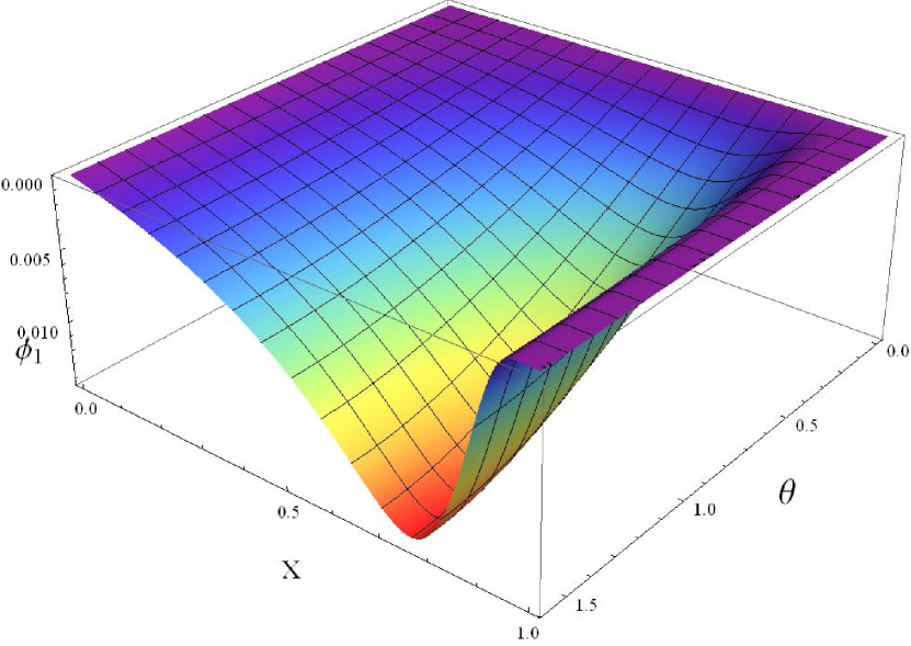
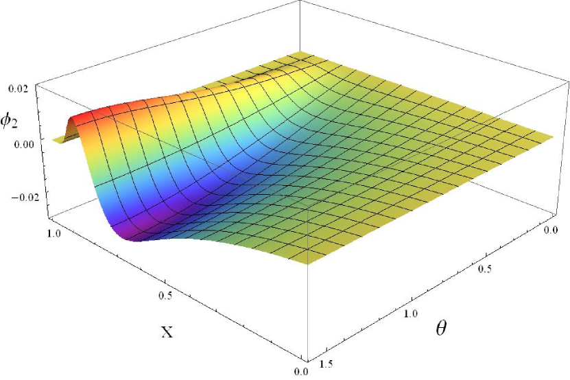
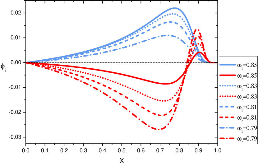
Figure 1: The distribution of the scalar field $\phi_{1}$ as a function of $x$ and $\theta$ (left panel) and the scalar $\phi_{2}$ as a function of $x$ and $\theta$ (middle panel) with the same parameter $\omega_{1}=\omega_{2}=0.8$, as well as the numerical solutions of the scalar fields $\phi_{i}$ $(i=1,2)$ versus the boundary $x$, represented by the blue and red lines, respectively and the horizon dashed black line represents the zero value (right panel). All solutions have $m_{1}=m_{2}=1$, $\mu_{1}=1$, and $\mu_{2}=0.93$.

Numerical results are presented in Fig. 1. We present the scalar field $\phi_{1}$ (left panel) and $\phi_{2}$ (middle panel) as a function of $x$ and $\theta$ with the azimuthal harmonic index $m_{1}=m_{2}=1$ for the same frequency $\omega_{1}=\omega_{2}=0.8$. The distribution of the scalar field $\phi_{1}$ (blue lines) and the scalar field $\phi_{2}$ (red lines) versus the boundary $x$ for several values of frequency $\omega_{1}=\omega_{2}$ are exhibited in the right panel of Fig. 1; we can observe that the scalar field $\phi_{2}$ changes sign once from the center of the boson stars to the boundary in a node. These behaviors are further shown in Fig. 2.

Meanwhile, to discuss the properties of the RMSBS, we also simplify our analysis; we mainly exhibit in Figs. 2 and  4 the mass $M$ and the angular momentum $J$ of several sets of the RMSBS versus the synchronized frequency $\omega$ and the nonsynchronized frequency $\omega_{2}$ with the azimuthal harmonic index $m_{2}=1~{},2,~{}3$.

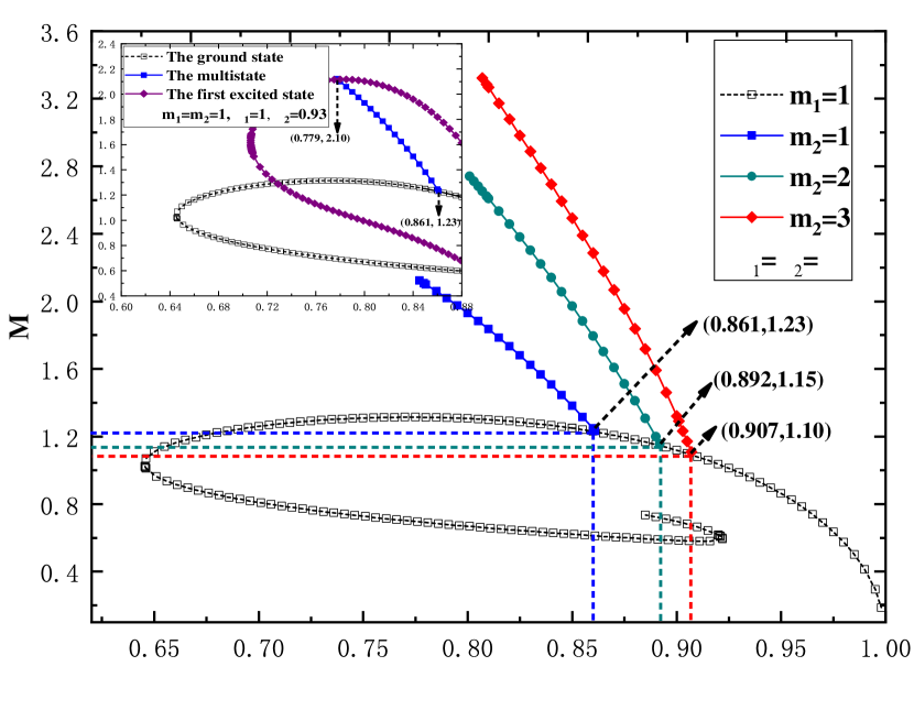
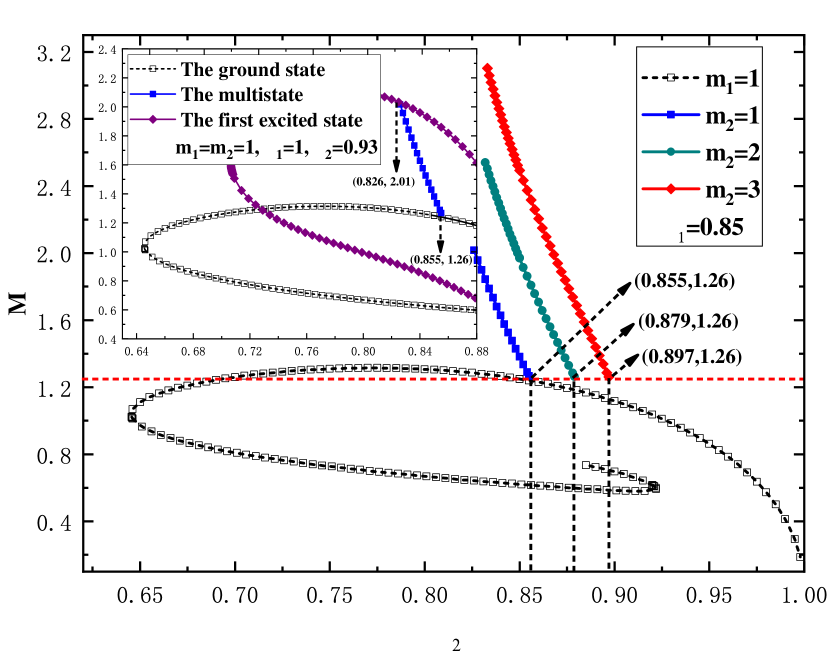
Figure 2: Left: The mass $M$ of the RMSBS as a function of the synchronized frequency $\omega$ with an azimuthal harmonic index $m_{2}=1~{},2,~{}3$. Three intersection points correspond to the coordinates $(0.861,~{}1.23)$, $(0.892,~{}1.15)$, and $(0.907,~{}1.10)$, respectively. Right: The mass $M$ of the RMSBS as a function of the nonsynchronized frequency $\omega_{2}$ with the fixed parameter $\omega_{1}=0.85$. The horizon red dashed line indicate the mass $M=1.26$, and the right ends of the blue, cyan, and red dotted lines correspond to the same value of $M$ with coordinates $(0.855,~{}1.26)$, $(0.879,~{}1.26)$, and $(0.897,~{}1.26)$, respectively. In both panels, the black hollowed line indicates the ground state solutions, and the inset of both panels show the ground state with $\mu_{1}=1$ (black line), the first excited state with $\mu_{2}=0.93$ (purple line), and the multistate with $\mu_{1}=1,\mu_{2}=0.93$ (blue line). All solutions have $m_{1}=1$.

The left panel of Fig. 2 exhibits the variation of the mass of the RMSBS versus the synchronized frequency $\omega$ with the azimuthal harmonic index $m_{2}=1~{},2,~{}3$, represented by the blue, cyan, and red lines, respectively, and the black hollowed line indicates the ground state with $m_{1}=1$. First observe that the domain of existence of the RMSBS are similar to the ground state boson stars in Ref. Herdeiro:2014goa . We again observe that as the synchronized frequency $\omega$ decreases, the mass of the RMSBS keeps increasing. In Ref. Herdeiro:2014goa , the behavior of the ground state solutions with $m_{1}=1$ spirals to the center; however, the RMSBS case does not occur with a second branch of unstable solutions with $m_{2}=1~{},2,~{}3$. In addition, we observe that, as the azimuthal harmonic index $m_{2}$ increases, the maximum value of the synchronized frequency $\omega$ also increases, and the minimum value of the mass of the RMSBS decreases as $m_{2}$ increases, and the multistate curves for $m_{2}=2,~{}3$ intersect with the ground state solutions with the coordinates $(0.892,~{}1.15)$ and $(0.907,~{}1.10)$, respectively. From the inset in left panel of Fig. 2, we can see that the curves of the ground state with $\mu_{1}=1$ (black), and first excited states with $\mu_{2}=0.93$ (purple). The multistate curve with $\mu_{1}=1,\mu_{2}=0.93$ (blue) intersects with the ground and first excited states with the coordinates $(0.861,~{}1.23)$ and $(0.779,~{}2.10)$, respectively. This means that when the synchronized frequency $\omega$ tends to its maximum, the first excited state could reduce to zero and there exists only a single the ground state. On the contrary, with the decrease of the synchronized frequency $\omega$, there exists only the first excited state.

In the right panel of Fig. 2, we plot the mass of the RMSBS versus the nonsynchronized frequency $\omega_{2}$ for the fixed value of $\omega_{1}=0.85$. One observes that, by increasing the azimuthal harmonic index $m_{2}$, the mass of the RMSBS keeps increasing. Meanwhile, as $\omega_{2}$ increases to its maximum, the minimum value of the mass of the RMSBS is the constant value $M=1.26$; three coordinates correspond to $(0.855,~{}1.26)$, $(0.879,~{}1.26)$, and $(0.897,~{}1.26)$, respectively. From the inset in right panel of Fig. 2, we show the ground state with $\mu_{1}=1$ (the black lines) and first excited states with $\mu_{2}=0.93$ (the purple lines). The multistate with $\mu_{1}=1,\mu_{2}=0.93$ (the blue line) intersects with the ground and first excited states with coordinates $(0.855,~{}1.26)$ and $(0.826,~{}2.01)$, respectively. That is, as the nonsynchronized frequency $\omega_{2}$ increases, the first excited state could decrease to zero and the mass of the RMSBS is provided by the ground state. On the contrary, with the decrease of the nonsynchronized frequency $\omega_{2}$, there exists only the first excited state. While we fixed the value of $\omega_{1}=0.85$, the minimal mass of the RMSBS is always a constant value $M=1.26$ for the different azimuthal harmonic indexes $m_{2}=2,~{}3$.

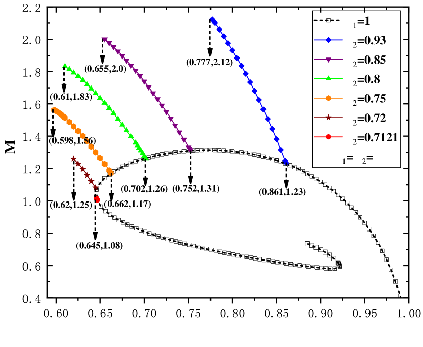
Figure 3: The mass $M$ of RMSBS as a function of synchronized frequency $\omega$ for the different values of $\mu_{2}$. The black hollowed line denotes the ground state with $\mu_{1}=1$, and all solutions have $m_{1}=m_{2}=1$ and $\mu_{1}=1$.

In order to verify whether there exists another family of multistate solutions between the ground state and the first excited state, we use two methods to seek for the new family of multistate solutions. The first way is that we adopt the similar method as the numerical algorithm given in Sec.VIIB of Dias:2015nua , and the second way is at the fixed $\mu_{1}=1$ where we change the values of $\mu_{2}$ to seek for the new family of multistate solutions for the same parameters. However, we fail to find the other family of multistate solutions in the maximum and minimum of the frequency for the cases of the ${}^{1}S^{2}S$ and ${}^{1}S^{2}P$ states. As an example in Fig. 3, the mass $M$ of RMSBS is a function of synchronized frequency $\omega$ for the different values of $\mu_{2}$. We observe that the domain of existence of the synchronized frequency $\omega$ decreases with the decrease of the scalar field mass $\mu_{2}$. Furthermore, when $\mu_{2}\rightarrow 0.7121$, the multistate curves approach the turning point of the ground state curves, and the synchronized frequency $\omega$ have a narrower range with $(0.646,~{}0.647)$. However, we fail to find the new family of multistate solutions between the ground state and the first excited state, but that does not mean there does not exist any new family of multistate solutions. At present, it is difficult for us to find out the other family of multistate solutions with numerical methods.

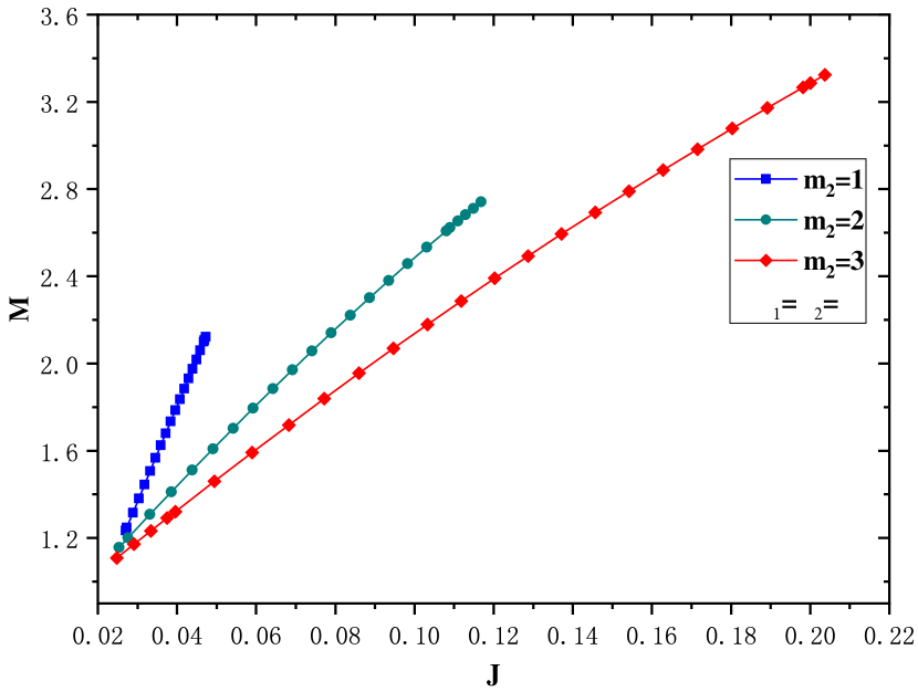
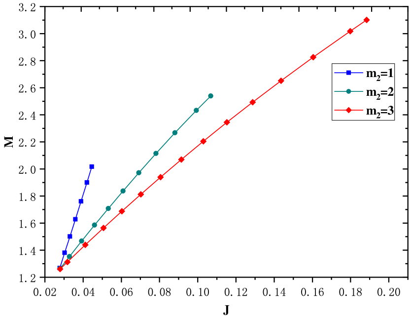
Figure 4: Left: The mass $M$ of the RMSBS versus the angular momentum $J$ for the synchronized frequency $\omega$ with $m_{2}=1~{},2,~{}3$ , respectively. Right: The mass $M$ of the RMSBS versus the angular momentum $J$ for the nonsynchronized frequency $\omega_{2}$ with $m_{2}=1~{},2,~{}3$, respectively, and we demand the parameter $\omega_{1}=0.85$.

Moving on with our analysis, we now consider the variation of the solutions with the mass $M$ of the rotating multistate boson stars that varies versus the angular momentum $J$, which is dependent on the frequency. In Fig. 4 (left panel), we exhibit the mass $M$ of the RMSBS versus the angular momentum $J$ with different azimuthal harmonic index $m_{2}=1$ (blue lines), 2 (cyan lines), and 3 (red lines) for the synchronized frequency $\omega$. In the right panel of Fig. 4, the mass $M$ versus the angular momentum $J$ with different azimuthal harmonic indexes $m_{2}=1~{},2,~{}3$ for the nonsynchronized frequency $\omega_{2}$ are shown, and we set the frequency parameter $\omega_{1}=0.85$. Comparing with the results of the ground state boson stars in Ref. Herdeiro:2014goa , we can see that the case of the RMSBS does not occur in zigzag patterns, and the minimum value of the mass $M$ is larger than that of the ground state boson stars.

Table 1: The domain of existence of the mass $\mu_{2}$ of the scalar field $\phi_{2}$ in three different situations: The synchronized frequency $\omega_{1}=\omega_{2}=\omega$ (left panel), the nonsynchronized frequency $\omega_{1}$ (middle panel), and the nonsynchronized frequency $\omega_{2}$ (right panel) with $m_{2}=1,2,3$, respectively. In the middle and right panels, we adopt $\omega_{2}=0.85$ and $\omega_{1}=0.85$, respectively. All solutions have $\mu_{1}=1$ and $m_{1}=1$.

	$1$	$2$	$3$
$0.78$	$0.874\sim 0.931$	$0.828\sim 0.920$	$0.803\sim 0.917$
$0.81$	$0.897\sim 0.944$	$0.859\sim 0.934$	$0.836\sim 0.931$
$0.84$	$0.917\sim 0.955$	$0.887\sim 0.947$	$0.868\sim 0.944$
$0.86$	$0.930\sim 0.962$	$0.905\sim 0.955$	$0.887\sim 0.953$
$0.88$	$0.942\sim 0.969$	$0.921\sim 0.963$	$0.906\sim 0.961$

(a)

	$1$	$2$	$3$
$0.70$	$1.058\sim 1.120$	$0.927\sim 1.080$	$0.879\sim 1.070$
$0.80$	$0.956\sim 1.004$	$0.910\sim 0.991$	$0.882\sim 0.986$
$0.84$	$0.930\sim 0.968$	$0.899\sim 0.959$	$0.878\sim 0.956$
$0.86$	$0.918\sim 0.951$	$0.893\sim 0.944$	$0.876\sim 0.942$
$0.88$	$0.907\sim 0.934$	$0.887\sim 0.929$	$0.873\sim 0.927$

(b)

	$1$	$2$	$3$
$0.83$	$0.899\sim 0.935$	$0.873\sim 0.928$	$0.855\sim 0.926$
$0.84$	$0.911\sim 0.947$	$0.884\sim 0.940$	$0.866\sim 0.937$
$0.85$	$0.924\sim 0.959$	$0.896\sim 0.951$	$0.878\sim 0.949$
$0.86$	$0.936\sim 0.971$	$0.908\sim 0.963$	$0.889\sim 0.960$
$0.88$	$0.959\sim 0.994$	$0.930\sim 0.985$	$0.911\sim 0.983$

In Table 1, we show the domain of existence of the mass $\mu_{2}$ of the scalar field $\phi_{2}$ in three different situations. The mass $\mu_{2}$ versus the synchronized frequency $\omega$ in Table 2(a), the nonsynchronized frequency $\omega_{1}$ in Table 2(b), and the nonsynchronized frequency $\omega_{2}$ in Table 1, as well as the three subtables have the same azimuthal harmonic index parameters $m_{2}=1~{},2,~{}3$, respectively.

In order to explore the influence of the different typical frequencies, the domain of existence of the mass $\mu_{2}$ with the azimuthal harmonic index parameter $m_{2}=1~{},2,~{}3$ for the same parameters $\omega=\omega_{1}=\omega_{2}=0.84~{},0.86,~{}0.88$ are shown. From Table 2(a), it is obvious that the domain of existence of the mass $\mu_{2}$ decreases with increasing synchronized frequency $\omega$. Again, by increasing the value of the azimuthal harmonic index parameter $m_{2}$, the mass domain as the synchronized frequency $\omega$ keeps increasing. In order to compare the results of the domain of existence of the mass $\mu_{2}$ of the scalar field $\phi_{2}$ versus the synchronized frequency $\omega$, we exhibit the domain of existence of the mass $\mu_{2}$ of the scalar field $\phi_{2}$ as a function of the nonsynchronized frequency $\omega_{1}$ in Table 2(b) and $\omega_{2}$ in Table 1 for the azimuthal harmonic index parameters $m_{2}=1~{},2,~{}3$. On the other hand, in Tables  2(b) and  1, the domain of existence of the mass $\mu_{2}$ with $m_{2}=1,~{}2,~{}3$ is similar to the case of synchronized frequency $\omega$ in Table 2(a), respectively.

IV.2 ${}^{1}S^{2}P$ state

In this subsection, we exhibit the solutions with one even-parity and one odd-parity scalar field. Along the angular $\theta$ and the radial $r$ directions, the scalar fields $\phi_{1}$ and $\phi_{2}$ also keep the same sign. Moreover, it is noted that the configuration with an odd parity are more unstable than the case with an even-parity scalar field Herdeiro:2015gia ; Wang:2018xhw . From the view of the excited states, these two states are just similar to the 1-s and 2-p states of the hydrogen atom, respectively.

IV.2.1 Boson star

In Fig. 5, we exhibit the scalar fields $\phi_{1}$ (left panel) and $\phi_{2}$ (middle panel) as a function of $x$ and $\theta$ with the azimuthal harmonic indexes $m_{1}=m_{2}=1$, $\omega_{1}=\omega_{2}=0.84$, and $\mu_{1}=1$ and $\mu_{2}=0.93$. The distribution of the scalar field $\phi_{1}$ (blue lines) and $\phi_{2}$ (red lines) versus the boundary $x$ for several values of the frequency $\omega_{1}=\omega_{2}$ are exhibited in the right panel of Fig. 5. Along the equatorial plane at $\theta=\pi/2$, we can see that the value of the scalar field $\phi_{2}$ tends to zero from the center of the boson stars to the boundary.

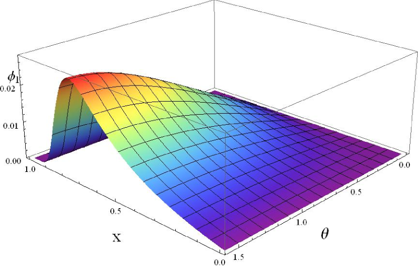
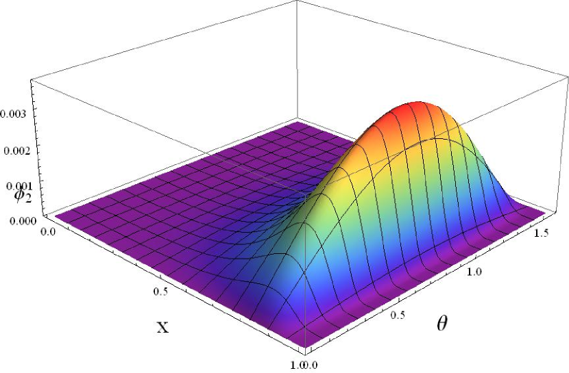
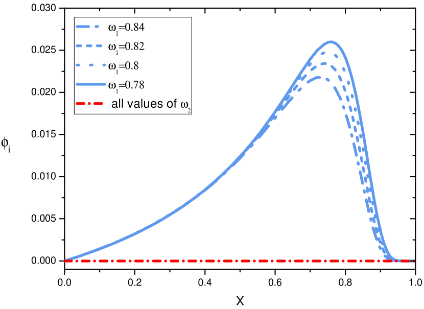
Figure 5: The distribution of the scalar field $\phi_{1}$ as a function of $x$ and $\theta$ (left panel) as well as the scalar $\phi_{2}$ as a function of $x$ and $\theta$ (middle panel) with the same frequency $\omega_{1}=\omega_{2}=0.84$. The numerical solutions of the scalar fields $\phi_{i}$ $(i=1,2)$ versus the boundary $x$ with an azimuthal harmonic index $m_{1}=1$, represented by the blue and red lines (right panel), respectively. All solutions have $m_{1}=m_{2}=1$, $\mu_{1}=1$, and $\mu_{2}=0.93$.

To discuss the properties of the RMSBS with the ${}^{1}S^{2}P$ state, we mainly exhibit in Fig. 6 the mass $M$ of the RMSBS versus the synchronized frequency $\omega$ and the nonsynchronized frequency $\omega_{2}$ with the azimuthal harmonic indexes $m_{2}=1~{},2,~{}3$.

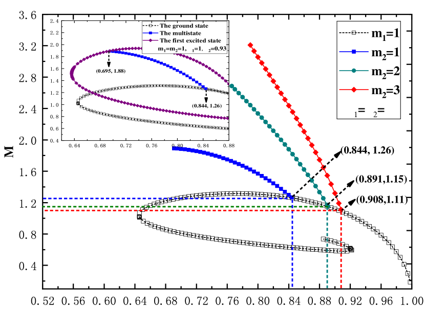
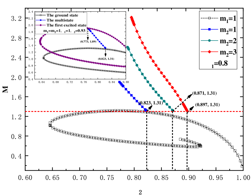
Figure 6: Left: The mass $M$ of the RMSBS as a function of the synchronized frequency $\omega$ with the azimuthal harmonic indexes $m_{2}=1~{},2,~{}3$. Three intersection points correspond to the coordinates $(0.844,~{}1.26)$, $(0.891,~{}1.15)$, and $(0.908,~{}1.11)$, respectively. Right: The mass $M$ of the RMSBS against the nonsynchronized frequency $\omega_{2}$ with the nonsynchronized frequency $\omega_{1}=0.8$. The horizon red dashed line indicate the mass $M=1.31$, and the right ends of the blue, cyan, and red dotted lines correspond to the same value of $M$ with coordinates $(0.823,~{}1.31)$, $(0.871,~{}1.31)$, and $(0.897,~{}1.31)$, respectively. In both panels, the black hollowed line indicates the ground state solutions, and the inset of both panels show the ground state with $\mu_{1}=1$ (black line), the first excited state with $\mu_{2}=0.93$ (purple line), and the multistate with $\mu_{1}=1,\mu_{2}=0.93$ (blue line). All solutions have $m_{1}=1$.

In the left panel of Fig. 6, we show the mass of the RMSBS versus the synchronized frequency $\omega$ with $m_{2}=1~{},2,~{}3$, represented by the blue, cyan, and red lines, respectively, and the black hollowed line indicates the ground state solutions for $m_{1}=1$. We found that the domain of existence of the RMSBS are similar to the ground state boson stars in Ref. Herdeiro:2014goa . Again, the mass of the RMSBS increases as the synchronized frequency $\omega$ decreases. The RMSBS case exhibits only a stable branch with $m_{2}=1~{},2,~{}3$, which is similar to the multistate with the ${}^{1}S^{2}S$ state. Besides, we note that, as the azimuthal harmonic index $m_{2}$ increases, this maximum value of the synchronized frequency $\omega$ decreases, and the minimum value of the mass of the RMSBS decreases as well. Hence, three sets of the RMSBS intersect with the ground state solutions for the coordinates $(0.844,~{}1.26)$, $(0.891,~{}1.15)$, and $(0.908,~{}1.11)$, respectively. From the inset in the left panel of Fig. 6, we note that the ground state with $\mu_{1}=1$ (the black lines), and the first excited states with $\mu_{2}=0.93$ (the purple lines). The multistate with $\mu_{1}=1,\mu_{2}=0.93$ (the blue line) intersect with the ground and first excited states with coordinates $(0.844,~{}1.26)$ and $(0.695,~{}1.88)$, respectively, which is similar to the multistate curves with the ${}^{1}S^{2}S$ state.

In the right panel of Fig. 6, we plot the mass of the RMSBS versus the nonsynchronized frequency $\omega_{2}$ for the $\omega_{1}=0.8$. We found that the mass of the RMSBS is increasing as $m_{2}$ increases. Moreover, by increasing $\omega_{2}$, the minimum value of the mass of the RMSBS is heavier than the case of the right panel of Fig. 2. Furthermore, from the inset in the right panel of Fig. 6, we also note that the detail of the curves of the ground state with $\mu_{1}=1$ (black) and the first excited states with $\mu_{2}=0.93$ (purple). The multistate curve with $\mu_{1}=1,\mu_{2}=0.93$ (blue) intersects with the ground and first excited states with coordinates $(0.773,~{}1.89)$ and $(0.823,~{}1.31)$, which is similar to the ${}^{1}S^{2}S$ state case. Because we fixed the value of $\omega_{1}=0.8$, the minimal mass of the RMSBS is always a constant value $M=1.31$ for the different azimuthal harmonic indexes $m_{2}=2,~{}3$. Thus, three coordinates correspond to $(0.823,~{}1.31)$, $(0.871,~{}1.31)$, and $(0.897,~{}1.31)$, respectively.

Table 2:   The domain of existence of the mass $\mu_{2}$ of the scalar field $\phi_{2}$ in three different situations: The synchronized frequency $\omega=\omega_{1}=\omega_{2}$ (left panel), the nonsynchronized frequency $\omega_{1}$ (middle panel) and the nonsynchronized frequency $\omega_{2}$ (right panel) with $m_{2}=1,2,3$, respectively. In the middle and right panels, we set $\omega_{1}=0.8$, $\omega_{2}=0.8$, respectively. All solutions have $\mu_{1}=1$ and $m_{1}=1$.

	$1$	$2$	$3$
$0.74$	$0.837\sim 0.950$	$0.771\sim 0.918$	$0.757\sim 0.910$
$0.78$	$0.881\sim 0.962$	$0.819\sim 0.936$	$0.811\sim 0.932$
$0.82$	$0.914\sim 0.972$	$0.864\sim 0.951$	$0.844\sim 0.945$
$0.84$	$0.928\sim 0.976$	$0.885\sim 0.958$	$0.864\sim 0.952$
$0.86$	$0.940\sim 0.980$	$0.904\sim 0.964$	$0.885\sim 0.959$

(a)

	$1$	$2$	$3$
$0.75$	$0.930\sim 1.026$	$0.843\sim 0.989$	$0.825\sim 0.978$
$0.80$	$0.898\sim 0.967$	$0.842\sim 0.943$	$0.823\sim 0.936$
$0.82$	$0.887\sim 0.946$	$0.840\sim 0.927$	$0.822\sim 0.921$
$0.84$	$0.876\sim 0.926$	$0.837\sim 0.910$	$0.821\sim 0.906$
$0.86$	$0.865\sim 0.908$	$0.834\sim 0.895$	$0.819\sim 0.891$

(b)

	$1$	$2$	$3$
$0.78$	$0.870\sim 0.941$	$0.818\sim 0.919$	$0.799\sim 0.912$
$0.80$	$0.898\sim 0.967$	$0.842\sim 0.943$	$0.822\sim 0.936$
$0.82$	$0.927\sim 0.994$	$0.866\sim 0.968$	$0.844\sim 0.961$
$0.84$	$0.956\sim 1.021$	$0.891\sim 0.993$	$0.866\sim 0.985$
$0.86$	$0.985\sim 1.048$	$0.916\sim 1.018$	$0.889\sim 1.009$

(c)

In Table 3(c), we present the domain of existence of the mass $\mu_{2}$ of the scalar field $\phi_{2}$ in three different situations. The mass $\mu_{2}$ versus the synchronized frequency $\omega$ in Table 3(a), the nonsynchronized frequency $\omega_{1}$ in Table 3(b) and the nonsynchronized frequency $\omega_{2}$ in Table 3(c). The three subtables have the same azimuthal harmonic index parameters $m_{2}=1~{},2,~{}3$, respectively. In Tables 3(a) and 3(c), the domain of existence of the mass $\mu_{2}$ with the azimuthal harmonic index parameters $m_{2}=1~{},2,~{}3$ for the same parameters $\omega=\omega_{2}=0.84~{},0.86,~{}0.88$ are shown. From Tables 3(a) and 3(c), we obvious that the domain of existence of the mass $\mu_{2}$ decreases with increasing synchronized frequency $\omega$ and nonsynchronized frequency $\omega_{2}$.

In addition, as the value of the azimuthal harmonic index parameter $m_{2}$ increases, the domain of existence of the mass $\mu_{2}$ also increases. In order to compare with the results of the domain of existence of the mass $\mu_{2}$ of the scalar field $\phi_{2}$ versus the synchronized frequency $\omega$, in Table 3(b), we exhibit the domain of existence of the mass $\mu_{2}$ with the nonsynchronized frequency $\omega_{1}$ for the azimuthal harmonic index parameters $m_{2}=1~{},2,~{}3$. We note that, for the values of the nonsynchronized frequencies $\omega_{1}=0.82$, $\omega_{1}=0.84$, and $\omega_{1}=0.86$ in Table 3(b), the domain of existence of the mass $\mu_{2}$ has the similar behavior as the case of ${}^{1}S^{2}S$ state in Table 2(b).

V Conclusion

In this paper, we have constructed and analyzed rotating boson stars composed of the coexisting states of two massive scalar fields, including the ground state and the first excited state. Comparing with the solutions of the rotating ground state boson stars in Ref. Herdeiro:2014goa , we have found that the RMSBS have two types of nodes, including the ${}^{1}S^{2}S$ state and the ${}^{1}S^{2}P$ state. By calculating the coexisting phase of the RMSBS for the two types of nodes, we found that the domain of existence of the mass $\mu_{2}$ decreases with an increasing synchronized frequency $\omega$, meanwhile, by increasing the value of the azimuthal harmonic index parameter $m_{2}$, the mass domain as the synchronized frequency $\omega$ keeps increasing. Furthermore, when the nonsynchronized frequency $\omega_{2}$ increases, the scalar field of the first excited state could decease to zero, and the minimal mass of the RMSBS is provided by the scalar field of the ground state. Therefore, the mass of the RMSBS is always a constant value for the different azimuthal harmonic indexes $m_{2}=1~{},2,~{}3$. In addition, from the numerical results, it is obvious that the mass of the RMSBS is heavier than the case of the ground state.

In order to better understand the stability properties of the RMSBS, according to the numerical analysis of the stability of the excited boson stars studied in Collodel:2017biu , the authors found the most stable solution will always belong to the set of ground state solutions, and for the case of nonrotating multistate boson stars Bernal:2009zy , the authors also found that there is a region of the solution space with stable configurations, that is, the deeper gravitational potential generated by the ground state, which is large enough to stabilize the excited state. It is worth to point out that it is difficult to numerically analyze the stability properties of rotating multistate boson stars. However, a good way to guarantee the stability of a specific solution is to have the linear perturbation mode in Ganchev:2017uuo .

Recently, motivation by the increasing interest in the models which consider scalar fields as viable dark matter candidates Sahni:1999qe ; Matos:2000ng ; Hu:2000ke ; Bernal:2016lll ; Padilla:2019fju has increased. For the ground state boson stars, these structures could produce rotation curves (RC), but the RC are not flat enough at large radii. Moreover, the excited state boson stars typically produce a more physically realistic, flatter RC, for which the solutions are unstable. In 2010, Bernal et al. Bernal:2009zy have obtained the configurations with two states, a ground and a first existed state, and they have demonstrated that the RC of multistate boson stars are flatter at large radii than the RC of single boson stars. As discussed above, the case of multistate boson stars is the spherically symmetric, nonrotating solutions. For the axisymmetric, rotating multistate solutions, however, we believe that the RC of rotating multistate boson stars also are flatter at large radii than the RC of single rotating solutions, and we hope that the RC of rotating multistate boson stars could be better used to accurately fit the rotation curves within the observational data. Therefore, we will calculate the rotation curves of rotating multistate boson stars in future work.

There are several interesting extensions of our work. Firstly, we have studied the rotating multistate boson stars; we would like to investigate how self-interactions of the scalar field affects the rotating multistate boson stars inspired by the work Kleihaus:2011sx . Secondly, the extension of our study is to construct the multistated Kerr black hole with scalar hairs, where two coexisting states of the scalar field are presented, including the ground and excited states. Finally, we are planning to numerically analyze of the linear stability properties of the rotating multistate boson stars in future work.

References

- (1) J. A. Wheeler, Geons, Phys. Rev. 97, 511 (1955).
- (2) E. A. Power and J. A. Wheeler, Thermal Geons, Rev. Mod. Phys. 29, 480 (1957).
- (3) R. Ruffini and S. Bonazzola, Systems of Self-Gravitating Particles in General Relativity and the Concept of an Equation of State, Phys. Rev. 187, 1767(1969).
- (4) D. J. Kaup, Klein-Gordon Geon, Phys. Rev. 172, 1331 (1968).
- (5) E. W. Mielke and R. Scherzer, Geon-type solutions of the nonlinear Heisenberg-Klein-Gordon equation, Phys. Rev. D 24, 2111 (1981).
- (6) M. Colpi, S. L. Shapiro, and I. Wasserman, Boson stars-Gravitational equilibria of self-interacting scalar fields, Phys. Rev. Lett. 57, 2485 (1986).
- (7) B. Hartmann, B. Kleihaus, J. Kunz, and I. Schaffer, Compact Boson Stars, Phys. Lett. B 714, 120 (2012).
- (8) S. Kumar, U. Kulshreshtha, and D. S. Kulshreshtha, Boson stars in a theory of complex scalar field coupled to gravity, Gen. Relativ. Gravit. 47, 76 (2015).
- (9) R. L. Guenther, A Numerical Study of the Time Dependent Schrodinger Equation Coupled with Newtonian Gravity, Ph.D. Thesis, University of Texas at Austin, 1995.
- (10) P. Jetzer and J. J. van der Bij, Charged boson stars, Phys. Lett. B 227, 341 (1989).
- (11) C. Dariescu and M. A. Dariescu, Boson Nebulae Charge, Chin. Phys. Lett. 27, 011101 (2010).
- (12) G. Murariu and G. Puscasu, Solutions for Maxwell-equations’ system in a static conformal space-time, Rom. J. Phys. 55, 47 (2010).
- (13) G. Murariu, C. Dariescu, and M. A. Dariescu, MAPLE Routines for Bosons on Curved Manifolds, Rom. J. Phys. 53, 99 (2008).
- (14) S. Kumar, U. Kulshreshtha, and D. S. Kulshreshtha, Charged compact boson stars and shells in the presence of a cosmological constant, Phys. Rev. D 94, 125023 (2016).
- (15) Y. Brihaye, T. Caebergs, and T. Delsate, Charged-spinning-gravitating Q-balls, arXiv:0907.0913.
- (16) A. B. Henriques, A. R. Liddle, and R. G. Moorhouse, Combined boson-fermion stars, Phys. Lett. B 233, 99 (1989).
- (17) A. B. Henriques, A. R. Liddle, and R. G. Moorhouse, Combined boson-fermion stars: Con- figurations and stability, Nucl. Phys. B 337, 737 (1990).
- (18) C. M. G. de Sousa, J. L. Tomazelli, and V. Silveira, Model for stars of interacting bosons and fermions, Phys. Rev. D 58, 123003 (1998).
- (19) F. Pisano and J. L. Tomazelli, Stars of WIMPs, Mod. Phys. Lett. A 11, 647 (1996).
- (20) A. Bernal, J. Barranco, D. Alic, and C. Palenzuela, Multi-state boson stars, Phys. Rev. D 81, 044031 (2010).
- (21) L. A. Urena-Lopez and A. Bernal, Bosonic gas as a Galactic dark matter halo, Phys. Rev. D 82, 123535 (2010).
- (22) S. H. Hawley and M. W. Choptuik, Numerical evidence for ‘multi-scalar stars’, Phys. Rev. D 67, 024010 (2003).
- (23) Y. Brihaye, T. Caebergs, B. Hartmann, and M. Minkov, Symmetry breaking in (gravitating) scalar field models describing interacting boson stars and Q-balls, Phys. Rev. D 80, 064014 (2009).
- (24) Y. Brihaye and B. Hartmann, Angularly excited and interacting boson stars and Q-balls, Phys. Rev. D 79, 064013 (2009).
- (25) L. G. Collodel, B. Kleihaus, and J. Kunz, Excited Boson Stars, Phys. Rev. D 96, 084066 (2017).
- (26) S. L. Liebling and C. Palenzuela, Dynamical boson stars, Living Rev. Relativity. 15, 6 (2012); 20, 5 (2017).
- (27) F. E. Schunck and E. W. Mielke, Rotating boson stars, in Relativity and Scientific Computing: Computer Algebra, Numerics, Visualization, 152nd WE-Heraeus seminar on edited by F. W. Hehl, R. A. Puntigam, and H. Ruder (Springer, Berlin, New York, 1996), pp. 138-151.
- (28) N. Kan and K. Shiraishi, Analytical Approximation for Newtonian Boson Stars in Four and Five Dimensions–A Poor Person’s Approach to Rotating Boson Stars, Phys. Rev. D 94, 104042 (2016).
- (29) S. Yoshida and Y. Eriguchi, Rotating boson stars in general relativity, Phys. Rev. D 56, 762 (1997).
- (30) O. J. C. Dias, G. T. Horowitz, and J. E. Santos, Black holes with only one Killing field, J. High Energy Phys. 07 (2011) 115.
- (31) I. Smolic, Symmetry inheritance of scalar fields, Classical. Quantum. Gravity. 32, , 145010 (2015).
- (32) C. A. R. Herdeiro, E. Radu, and H. F. Rúnarsson, Spinning boson stars and Kerr black holes with scalar hair: the effect of self-interactions, Int. J. Mod. Phys. D 25, 1641014 (2016).
- (33) T. D. Lee and Y. Pang, Stability of mini-boson stars, Nucl. Phys. B315, 477 (1989).
- (34) B. Kleihaus, J. Kunz, and S. Schneider, Stable phases of boson stars, Phys. Rev. D 85, 024045 (2012).
- (35) F. V. Kusmartsev, E. W. Mielke, and F. E. Schunck, Gravitational stability of boson stars, Phys. Rev. D 43, 3895 (1991).
- (36) F. V. Kusmartsev and F. E. Schunck, Analogies and differences between neutron and boson stars studied with catastrophe theory, Physica (Amsterdam) 178B, 24 (1992), https://doi.org/10.1016/0921-4526(92)90175-R.
- (37) C. Herdeiro and E. Radu, Construction and physical properties of Kerr black holes with scalar hair, Classical. Quantum. Gravity. 32, 144001 (2015).
- (38) C. A. R. Herdeiro and E. Radu, Kerr black holes with scalar hair, Phys. Rev. Lett. 112, 221101 (2014).
- (39) B. Ganchev and J. E. Santos, Scalar Hairy Black Holes in Four Dimensions are Unstable, Phys. Rev. Lett. 120, 171101 (2018).
- (40) J. C. Degollado, C. A. R. Herdeiro, and E. Radu, Effective stability against superradiance of Kerr black holes with synchronised hair, Phys. Lett. B 781, 651 (2018).
- (41) S. Hod, Stationary scalar clouds around rotating black holes, Phys. Rev. D 86, 104026 (2012).
- (42) C. L. Benone, L. C. B. Crispino, C. Herdeiro, and E. Radu, Kerr-Newman scalar clouds, Phys. Rev. D 90, 104024 (2014).
- (43) C. Herdeiro, E. Radu and H. Rúnarsson, Kerr black holes with Proca hair, Classical. Quantum. Gravity. 33, 154001 (2016).
- (44) J. F. M. Delgado, C. A. R. Herdeiro, E. Radu, and H. Runarsson Kerr-Newman black holes with scalar hair, Phys. Lett. B 761, 234 (2016).
- (45) C. A. R. Herdeiro and E. Radu, Spinning boson stars and hairy black holes with nonminimal coupling, Int. J. Mod. Phys. D 27, 1843009 (2018).
- (46) C. Herdeiro, I. Perapechka, E. Radu, and Y. Shnir, Skyrmions around Kerr black holes and spinning BHs with Skyrme hair, J. High Energy Phys. 10 (2018) 119.
- (47) W. E. East and F. Pretorius, Superradiant Instability and Backreaction of Massive Vector Fields around Kerr Black Holes, Phys. Rev. Lett. 119, 041101 (2017).
- (48) C. A. R. Herdeiro and E. Radu, Asymptotically flat black holes with scalar hair: A review, Int. J. Mod. Phys. D 24, 1542014 (2015).
- (49) Y. Q. Wang, Y. X. Liu, and S. W. Wei, Excited Kerr black holes with scalar hair, Phys. Rev. D 99, 064036 (2019).
- (50) J. Kunz, I. Perapechka, and Y. Shnir, Kerr black holes with parity-odd scalar hair, Phys. Rev. D 100, 064032 (2019).
- (51) J. F. M. Delgado, C. A. R. Herdeiro, and E. Radu, Kerr black holes with synchronised scalar hair and higher azimuthal harmonic index, Phys. Lett. B 792, 436 (2019).
- (52) J. Kunz, I. Perapechka, and Y. Shnir, Kerr black holes with synchronised scalar hair and boson stars in the Einstein-Friedberg-Lee-Sirlin model, J. High Energy Phys. 07 (2019) 109.
- (53) O. J. C. Dias, J. E. Santos and B. Way, Numerical Methods for Finding Stationary Gravitational Solutions, Classical. Quantum. Gravity. 33, 133001 (2016).
- (54) V. Sahni and L. M. Wang, A new cosmological model of quintessence and dark matter, Phys. Rev. D 62, 103517 (2000).
- (55) T. Matos and L. A. Urena-Lopez, Quintessence and scalar dark matter in the universe, Classical. Quantum. Gravity. 17, L75 (2000).
- (56) W. Hu, R. Barkana, and A. Gruzinov, Cold and Fuzzy Dark Matter, Phys. Rev. Lett. 85, 1158 (2000).
- (57) T. Bernal, V. H. Robles, and T. Matos, Scalar field dark matter in clusters of galaxies, Mon. Not. R. Astron. Soc. 468, 3135 (2017).
- (58) L. E. Padilla, J. A. Vázquez, T. Matos, and G. Germán, Scalar field dark matter spectator during inflation: The effect of self-interaction, J. Cosmol. Astropart. Phys. 05 (2019) 056.